A Neural Network-Based Analysis of the Seasonal Variability of Surface Total Alkalinity on the East China Sea Shelf

Introduction

Despite occupying a small proportion of the global surface area, coastal seas play an important role in the global carbon cycle because they receive a large amount of terrestrial materials and nutrients from rivers, rapidly transform different forms of carbon, and exchange large fluxes with the open ocean and atmosphere (Gattuso et al., 1998). It has been suggested that coastal seas may contribute greatly to the absorption of atmospheric carbon dioxide (e.g., Borges et al., 2005; Cai et al., 2006), and are more sensitive to global climate changes and anthropogenic influences such as global warming, eutrophication and ocean acidification (e.g., Doney et al., 2007; Cai et al., 2011; Omar et al., 2019). However, the carbonate system in the coastal oceans can change in an unpredictable way under multiple environmental stressors, and observational datasets often lack carbonate chemistry measurements or include only one carbonate chemistry parameter, while at least two are needed to fully characterize the seawater carbonate system (Millero, 2007).

Several studies have attempted to develop multiple linear regression (MLR) relationships to predict total alkalinity (A_T) from more commonly observed variables such as temperature and salinity (e.g., Millero et al., 1998; Lee et al., 2006; Carter et al., 2016, 2018; Fine et al., 2017). However, it has proved difficult to find such relationships that maintain accuracy over large scales. A new method of self-organizing multiple linear output (SOMLO) was developed by Sasse et al. (2013), and showed a 19% improvement in predictive accuracy for dissolved inorganic carbon compared to a traditional MLR approach. Superior predictors have also been obtained using self-organizing maps (Velo et al., 2013) or neural networks (e.g., Sauzède et al., 2017; Broullón et al., 2019). To date, however, relatively few studies have attempted to develop A_T predictors specifically for coastal regions, perhaps because of the complexity and heterogeneity of the continental shelves. Alin et al. (2012) developed an MLR model for A_T in the southern California Current System, while Gemayel et al. (2015) derived polynomial fits to estimate A_T in the Mediterranean Sea. As discussed by Friis et al. (2003), simple linear regressions between salinity and A_T may not be suitable for broader coastal ocean regions. Numerous processes in the coastal seas lead to the complexity of carbonate system dynamics, which means that each specific region may have different variation characteristics of A_T in different seasons and separate, regional algorithms may be required (e.g., Juranek et al., 2009; Kim et al., 2010).

The East China Sea (ECS) is the largest marginal sea in the western North Pacific Ocean and receives massive terrestrial inputs from the Changjiang River (Gong et al., 1996). Hur et al. (1999) investigated the monthly water mass variations in the ECS using more than 40 years of historical data and a cluster analysis approach. In order to reveal the seasonal variations of major water masses in the ECS, Li et al. (2006) proposed a simple spiciness index and found that monthly variations of the water masses can be classified into three phases per year. Spatial and temporal distributions of carbonate system parameters have also been investigated in the ECS (e.g., Chou et al., 2009, 2013; Qu et al., 2015, 2017), and were found to largely reflect the distributions of various water masses in the ECS. The pattern of carbon sources and sinks exhibits substantial seasonal variation (Guo et al., 2015), and the ECS is generally considered as a sink of atmospheric CO₂ throughout the year except in fall (e.g., Shim et al., 2007; Zhai and Dai, 2009). However, the seasonal variability of A_T in the ECS has been very little studied, mainly due to the limited observational coverage. Developing methods to extend the seasonal coverage of A_T data may thus help to improve our understanding of the ocean carbon cycle in the ECS.

Artificial neural networks (ANNs) have been proposed as powerful tools for modeling uncertain and complex systems such as ecosystems and for environmental assessment (e.g., Olden and Jackson, 2002; Olden et al., 2004; Uusitalo, 2007; Raitsos et al., 2008). Their main advantage compared with MLR models is that they do not require an a priori model but rather “learn” the model from training data (e.g., Hornik et al., 1989; Raitsos et al., 2008). ANNs have been used to retrieve the partial pressure of carbon dioxide (pCO₂) (e.g., Friedrich and Oschlies, 2009; Laruelle et al., 2017), A_T (e.g., Bostock et al., 2013; Sasse et al., 2013; Velo et al., 2013), and dissolved inorganic carbon (e.g., Bostock et al., 2013; Sasse et al., 2013). To our knowledge, no empirical relationship for A_T has yet been developed for the ECS shelf, likely due to the limited observations and the complex interaction of different water masses.

We developed an ANN to predict A_T on the ECS shelf and used it to investigate seasonal variability. This paper is structured as follows: section “Materials and Methods” introduces the research region and cruise data used to build the ANN; section “Results and Discussion” shows the ANN model performance, variable importance in the ANN model, and two applications: to calculate surface A_T for 8 cruises on the ECS shelf during 2013–2016 using in situ measured temperature, salinity and dissolved oxygen; to retrieve monthly A_T for the period 2000–2016 on the ECS shelf using the monthly temperature, salinity, and dissolved oxygen from the Changjiang Biology Finite-Volume Coastal Ocean Model (FVCOM) Data. Conclusions and perspectives are summarized in the last section.

Materials and Methods

Study Area and Observations

The ECS is framed by the Ryukyu Island chain in the east (Japan), mainland China in the west, Taiwan in the south, and Cheju Island (Korea) in the north. The winter monsoon from the north lasts from September to April, while the summer monsoon from the south lasts from July to August (Lee and Chao, 2003). The Changjiang Diluted Water (CDW) spreads eastward in summer during the prevailing southwest monsoon, while it is confined to the western side of the shelf under the influence of the northeast monsoon (Chou et al., 2009, 2013). The Taiwan Warm Current (TWC) flows into the ECS through the Taiwan Strait, the Kuroshio Current (KC) flows northeast along the shelf break (e.g., Lee and Chao, 2003; Chou et al., 2009), and the Yellow Sea Coastal Current (YSCC) enters the northern part of the ECS under the influence of the northeast monsoon (Gong et al., 1996).

Four cruises were conducted in the ECS from 2017 to 2018. Three cruises were carried out during the “National Natural Science Foundation Shared Voyage Plan,” from 10 to 19 March 2018, 12–20 July 2018, 12–21 October 2018; the remaining cruise was carried out during “Vulnerabilities and Opportunities of the Coastal Ocean” on the ECS shelf during 12–24 May 2017. Water samples were collected at three or four different depths during all cruises. One additional cruise dataset from 2 to 9 January 2008 in the ECS has been reported previously by Chou et al. (2011) and was downloaded from the Carbon Dioxide Information Analysis Center¹. Temperature (T) and salinity (S) profiles were obtained directly using a conductivity temperature-depth/pressure (CTD) recorders (SBE 25plus or 911plus). Measurement of dissolved oxygen (DO) followed the Winkler procedure, as described previously by Zhai et al. (2014b). A_T samples were potentiometrically titrated with standardized 0.1 M HCl (0.7 M in NaCl) to the carbonic acid end point using a VINDTA 3C system, as described by Mintrop et al. (2000). Certificated Reference Materials (CRMs) were used to determine a precision of ± 2 μmol kg^–1 (Dickson et al., 2007). The final number of data used by the ANN model was 699, and the distribution of the sampling sites from the five cruises is shown in Figure 1.

FIGURE 1

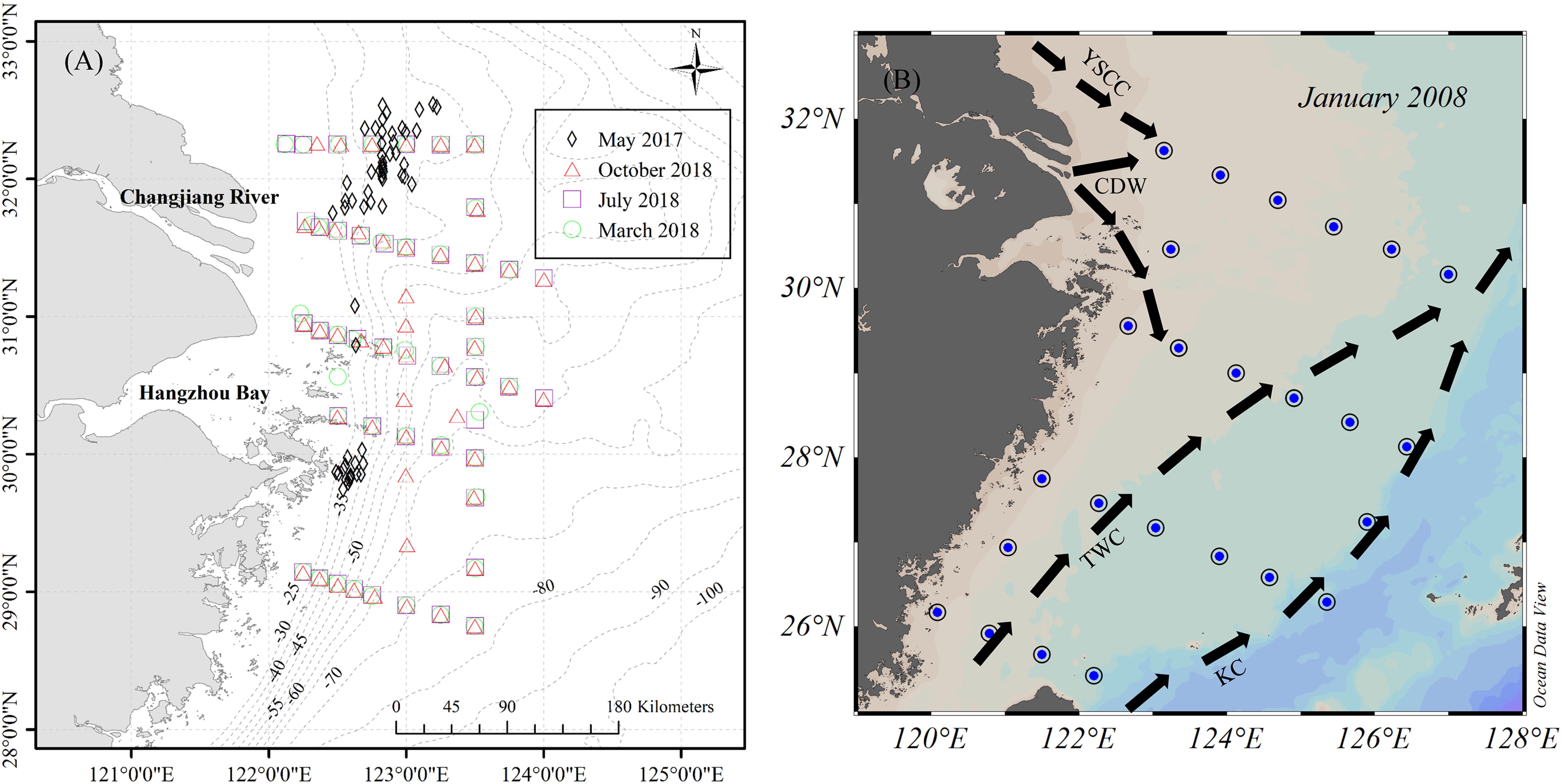
Figure 1. Sampling stations during five cruises on the ECS shelf. (A) The black diamond, red triangle, purple square, and green circle represent May 2017, October 2018, July 2018, and March 2018, respectively; (B) January 2008 cruise reported by Chou et al. (2011). CDW, Changjiang Dilute Water; TWC, Taiwan Warm Current; KC, Kuroshio Current; YSCC, Yellow Sea Coastal Current.

Artificial Neural Network Development

Similar to the input variables selected by Bostock et al. (2013), we selected T, S, and DO as predictors into the ANN model. The input variables also included the sampling position (longitude and latitude) and sampling time (month). The sampling position and time were included to help the network to learn spatio-temporal patterns that cannot be explained by other input variables (Sasse et al., 2013). The ANN we used is a feed-forward multilayer perceptron (Tamura and Tateishi, 1997) with two hidden layers. The neurons of each layer are connected with the neurons of the previous layer and the next layer by weights (Figure 2). The coefficients of the weight matrix are iteratively tuned in the training step. Here we used the back-propagation conjugate-gradient technique (Hornik et al., 1989). In order to avoid overfitting, a ten-fold cross-validation was used to assess model prediction accuracy. In this technique, all cruises data was randomly divided into ten equal subsamples. One subsample was used as the independent validation data (10% of all data), which was always excluded from training, and the nine remaining subsamples were together used as training data (90% of all data). Within the training data, the data was further divided randomly into a training set (70% of training data), validation set (15% of training data), and testing set (15% of training data). We compared performance in predicting the independent validation data from the ten-fold cross-validation and selected the optimal model based on the lowest root mean square error. All calculations were done in the MathWorks Matlab environment.

FIGURE 2

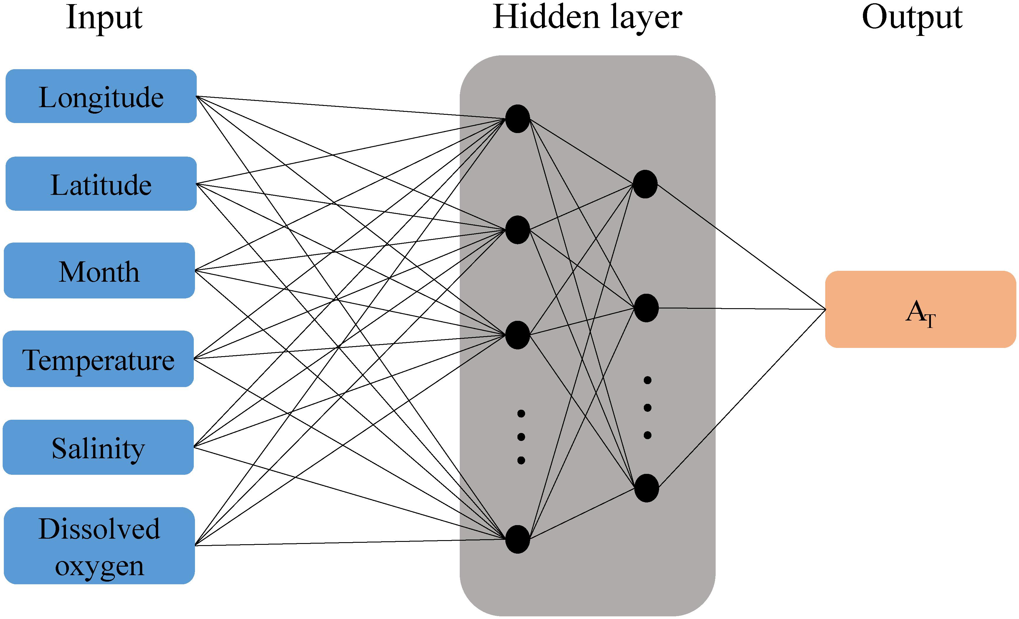
Figure 2. Schematic representation of the neural network algorithm to retrieve total alkalinity. Input variables are observed temperature, salinity, and dissolved oxygen together with the geolocation (longitude and latitude) and time (month) of sampling.

There is no fixed criterion to set up the optimal number of neurons in the two hidden layers, which was tested varying between 1 and 30, respectively (Table 1). The optimal architecture was composed of two hidden layers with twenty neurons in the first and twelve neurons in the second. In order to avoid bias toward high-value inputs/outputs and to eliminate the dimensional influence of the data, all data used by the ANN model were normalized using the following equation (e.g., Sauzède et al., 2015, 2016):

TABLE 1

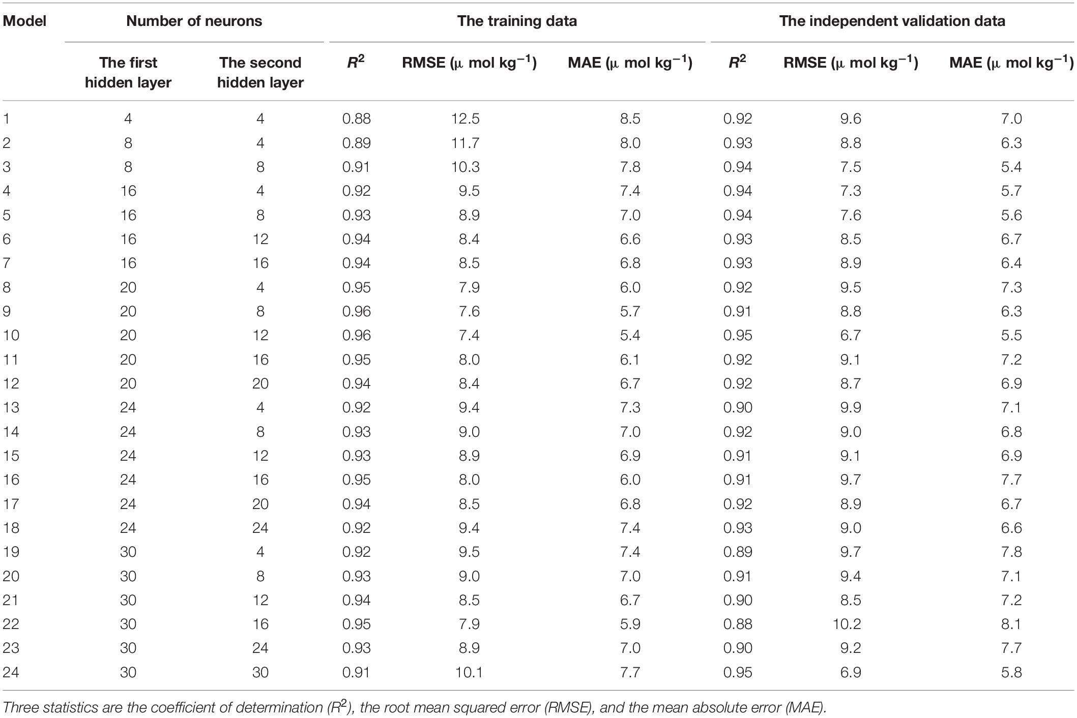
Table 1. Different model structures and their performance in the training step.

$$x_{i,j}=\frac{2}{3}\ast \frac{x_{i,j}-mean(x_{i,j})}{\mathrm{\sigma }(x_{i,j})}(1)$$

with σ the standard deviation of the considered input variable or the output variable A_T. Similar to the approach of Sauzède et al. (2015, 2016), the longitude and month input variables were transformed as follows to account for periodicity:

$$\text{slongitude}=\sin \left({\displaystyle \frac{Lon\ast \pi }{180}}\right),\text{clongitude}=\cos \left({\displaystyle \frac{Lon\ast \pi }{180}}\right)(2)$$

$$\text{smonth}=\sin \left({\displaystyle \frac{month\ast \pi }{6}}\right),\text{cmonth}=\cos \left({\displaystyle \frac{month\ast \pi }{6}}\right)(3)$$

The latitude variable was transformed into the range of the sigmoid function (Sauzède et al., 2015) by divided by 90, then was processed using Equation (1).

Results and Discussion

The ANN Model Performance

To evaluate the performance of the ANN model, we compared the model retrieved A_T (A_TM) with corresponding observations (A${}_{\text{T}}^{\text{O}}$) using several statistical indices: the mean absolute error (MAE), the coefficient of determination (R²), and the root mean squared error. The model simulated A_T with RMSE = 7.4 μmol kg^–1 and R² = 0.96 for the training data (90% of all data, Figure 3A), and predicted A_T with RMSE = 6.7 μmol kg^–1 and R² = 0.95 for the independent validation data (10% of all data, Figure 3B). The normal distribution of the differences (A_TM – A${}_{\text{T}}^{\text{O}}$) shows that only a few points exceed ±2RMSE (Supplementary Figure S1), and 52% of our model determinations are within the normal accuracy for A_T measurements (internationally) ± 4 μmol kg^–1. Supplementary Figure S4 shows the performance of model extrapolation for longitude and month.

FIGURE 3

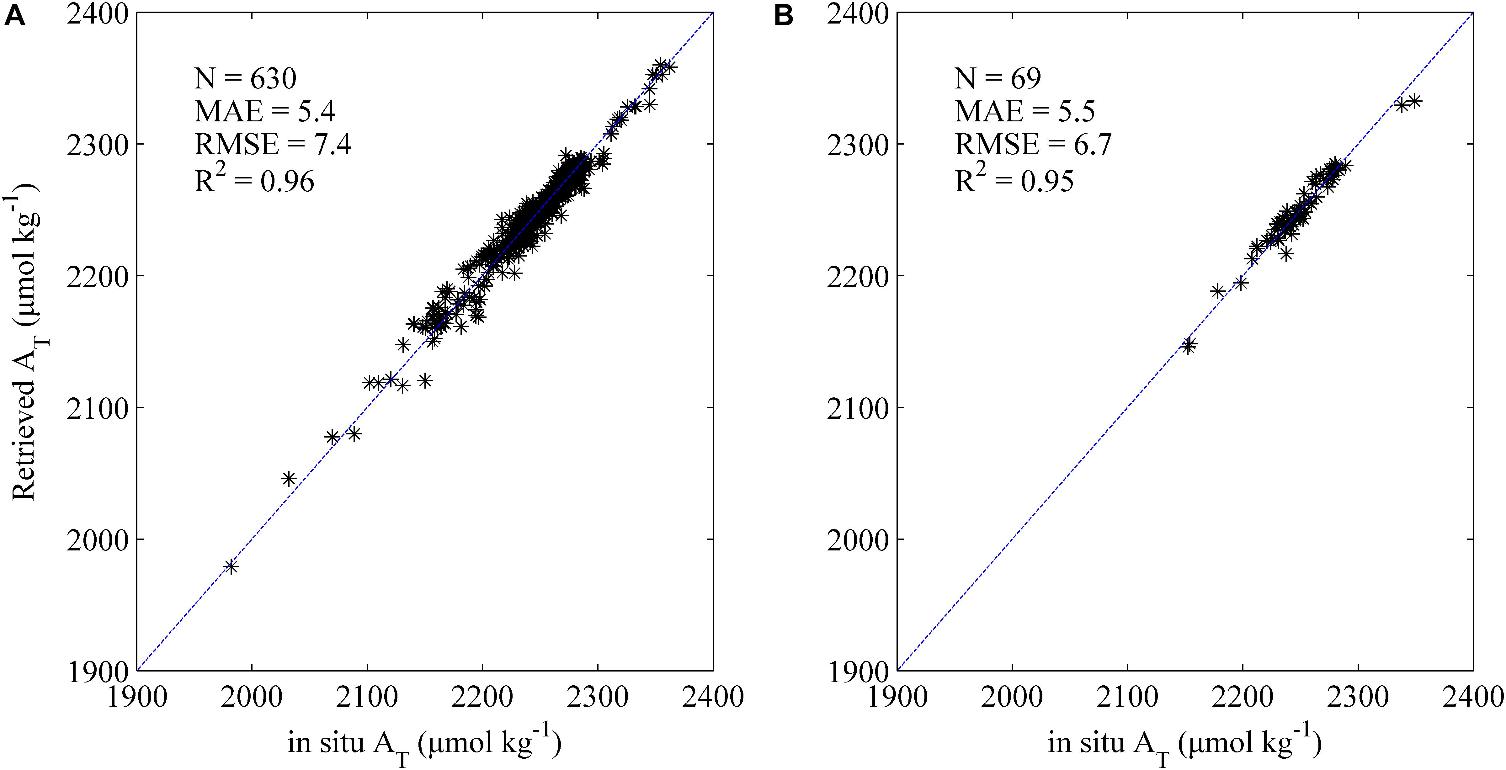
Figure 3. Comparison of A_T retrieved by the ANN model with corresponding observations. (A)-training data (90% of all data); (B)-independent validation data (10% of all data). The 1:1 line is shown in each plot as visual reference. N represents the number of data points. Three statistics are the mean absolute error (MAE), the root mean squared error (RMSE), and the coefficient of determination (R²).

In order to further explore where the ANN model result in differences beyond ±2RMSE, we plotted the distribution of the differences larger than ±2RMSE against longitude and latitude (Figure 4). These points are concentrated in an area strongly influenced by Changjiang River runoff, Yellow Sea Coastal Current (YSCC) and shelf seawater, and the wet season (May and July), during which Changjiang River is in flood (Supplementary Figure S2). The reduced performance of the ANN model can be primarily attributed to the sudden increase in the Changjiang River discharge and appearance of seawater vertical stratification during the wet season. During this special period, large amounts of nutrients inputs from the Changjiang River can stimulate primary production, seawater vertical stratification can hinder material exchange in the water column, and massive freshwater input can suddenly reduce salinity, all of which poses a challenge for empirical modeling.

FIGURE 4

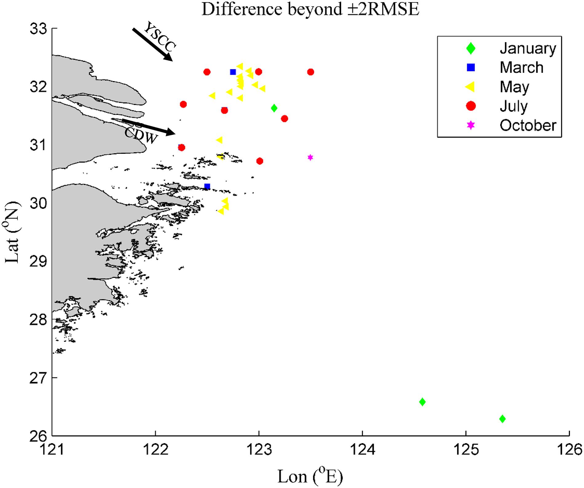
Figure 4. Scatter diagram of the differences beyond ±2RMSE between total alkalinity estimated by the ANN model minus the observations for all cruises data.

Although the RMSE of 7.4 μmol kg^–1 for A_T we obtained here was higher than the 6.4 μmol kg^–1 obtained by Alin et al. (2012), it was lower than obtained in other previous studies. For example, Evans et al. (2013) derived a MLR to estimate A_T with RMSE of 9 μmol kg^–1 in the northern Gulf of Alaska, Gemayel et al. (2015) presented polynomial fits to predict A_T with RMSE of 10.6 μmol kg^–1 in the Mediterranean Sea. In addition, an empirical relationship between A_T and S was established for all seasons with the residual of 17 μmol kg^–1 in the Washington State Coastal Zone (Fassbender et al., 2017). Furthermore, relationships between T and S with A_T by Lee et al. (2006) were applied to compute surface A_T with RMSE of 17.6 μmol kg^–1 (Figure 5), which suggests that this relationship fails to compute A_T in this shallow sea with the high river runoff and the ANN model is a better approach than Lee et al. (2006) on the ECS shelf.

FIGURE 5

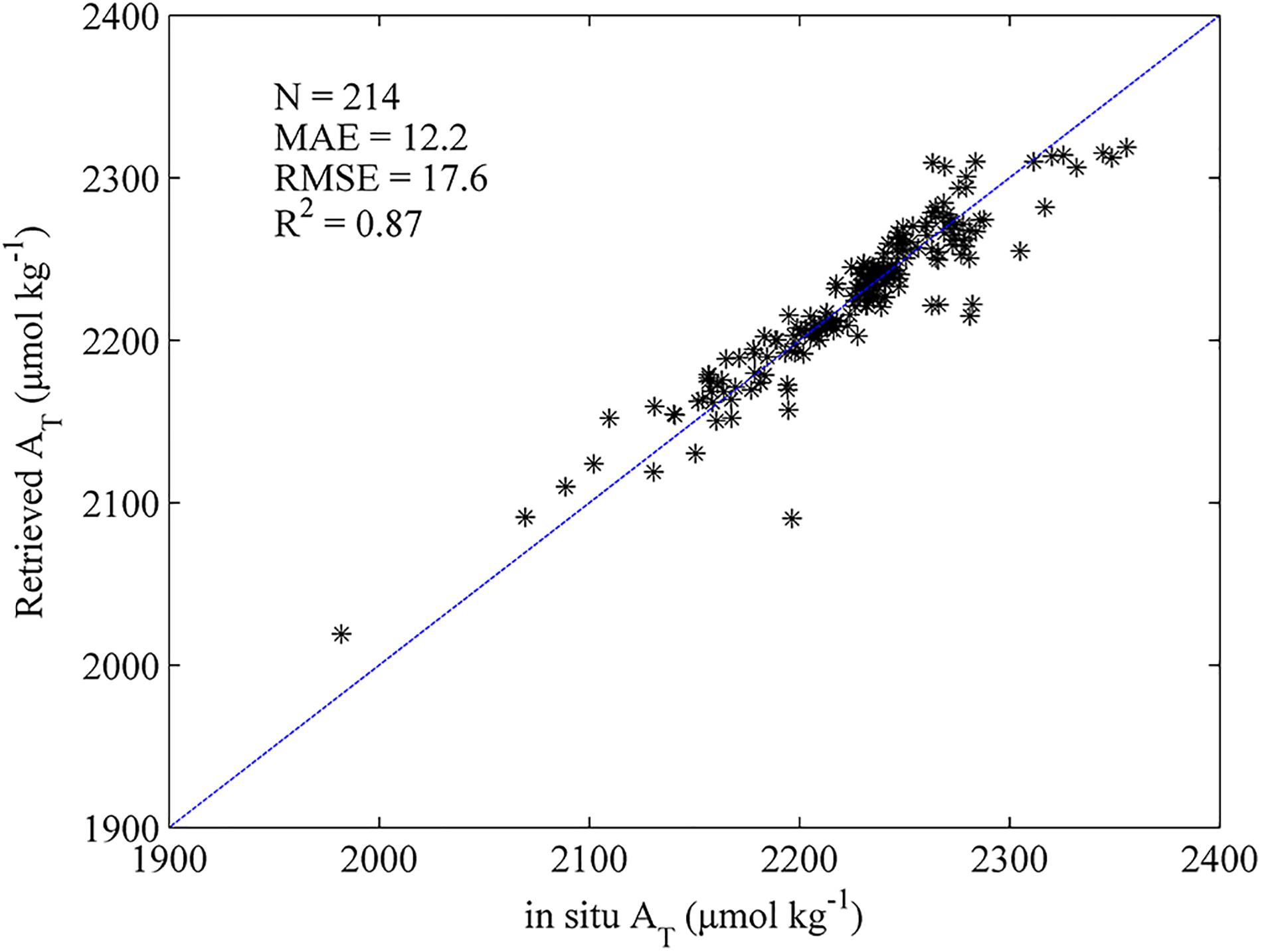
Figure 5. Comparison of A_T retrieved by the relations of Lee et al. (2006) with corresponding surface observations. The 1:1 line is shown in each plot as visual reference. N represents the number of surface data points. Three statistics are the mean absolute error (MAE), the root mean squared error (RMSE), and the coefficient of determination (R²).

Variable Importance in the ANN Model

To quantitatively estimate input variables that affect A_T in the ANN model, we used the following method: for each input variable separately, add 5% and calculate the resulting percentage change in the predicted A_T. The A_T is positively correlated with salinity and longitude, and negatively correlated with temperature (Figure 6). The two variables with the greatest weight are salinity and longitude, and the weights of other variables are small and can almost be ignored when compared with salinity and longitude. The significant positive correlation between A_T and salinity was also found by Zhai et al. (2014a). The positive correlation between A_T and longitude reflects the distribution pattern of A_T in space, which is similar to salinity and generally increasing eastward from the China coastline to the shelf break (e.g., Chou et al., 2013; Qu et al., 2017).

FIGURE 6

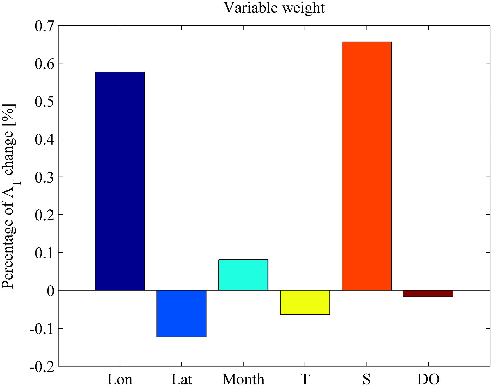
Figure 6. Variable importance estimates in the ANN model. For each input variable separately, add 5% and calculate the resulting percentage change in the predicted A_T.

Model Applications

In order to retrieve A_T on the ECS shelf, the monthly T, S, and DO from the Changjiang Biology Finite-Volume Coastal Ocean Model (FVCOM) Data² were applied to the ANN model as the input variables. The performance of monthly T, S, and DO from the Changjiang Biology FVCOM model was shown in Supplementary Figure S3. Monthly A_T for the period 2000–2016 was obtained at the spatial resolution of the FVCOM output: 1–10 km in the horizontal, 10 depth levels in the vertical, and 12 months. Also, since A_T was not measured during 8 cruises from 2013 to 2016 on the ECS shelf, the surface A_T was retrieved through the ANN model using in situ measured T, S, and DO.

Surface Total Alkalinity Retrieved From Cruise Observations

The distributions of retrieved A_T in winter and summer from 2013 to 2016 are shown in Figure 7. The distribution characteristics of A_T we calculated in 2013–2016 are consistent with that of A_T previously published in other years during summer and winter (e.g., Chou et al., 2009, 2011; Qu et al., 2015, 2017). In winter, high A_T is found in the north of the study area, related with the YSCC, while low A_T is confined to a narrow coastal region (water depth <50 m), controlled by the prevailing northeast monsoon. In summer, high A_T is found in the eastern and southeastern parts of the study area, related with the intrusion of the TWC and the KC, while low A_T is confined mainly to the western and northwestern parts of the study area, influenced by the CDW and the southwest monsoon.

FIGURE 7

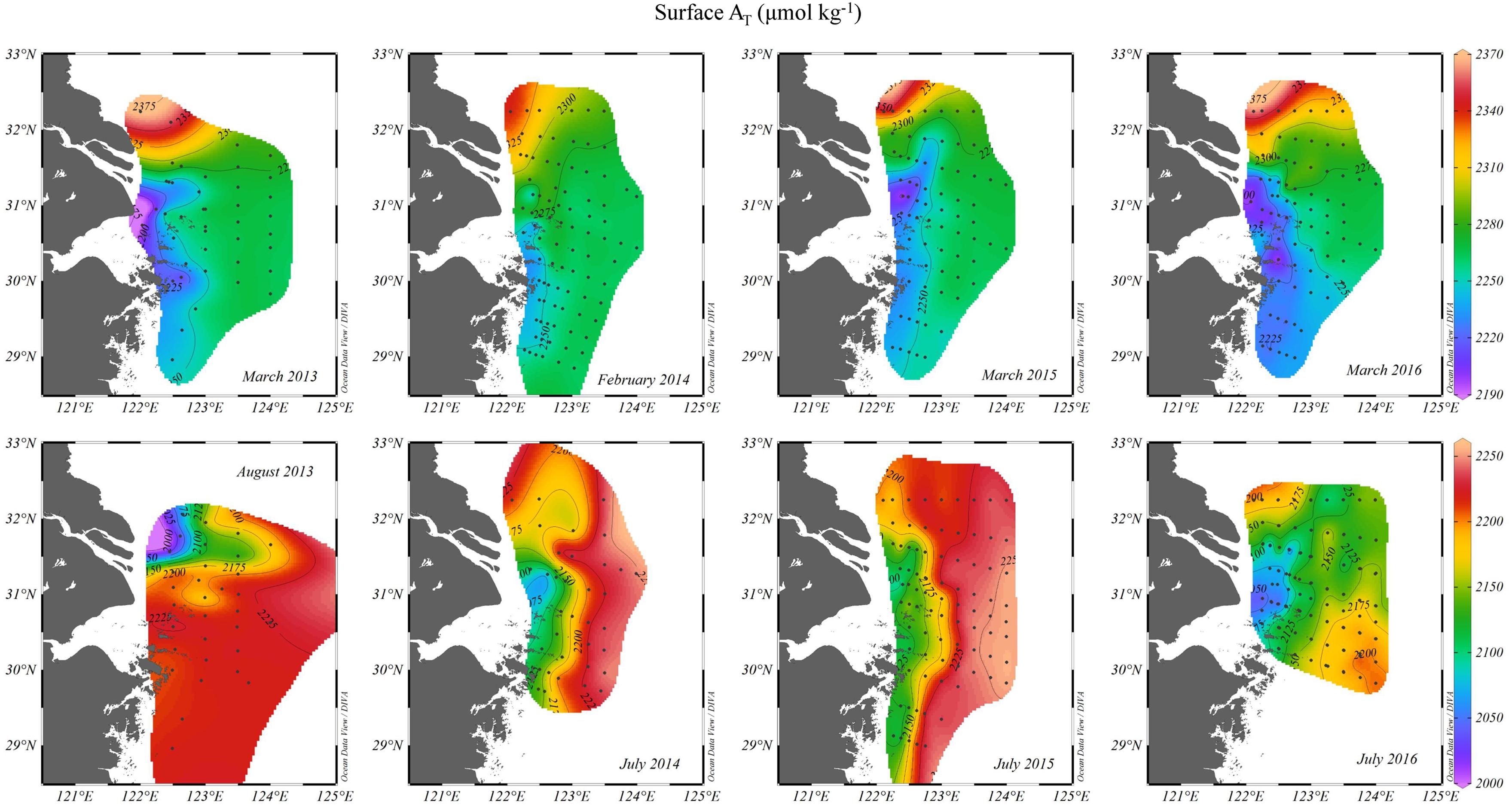
Figure 7. Spatial distribution of surface ANN-derived A_T of eight cruises from 2013 to 2016 on the ECS shelf.

Surface Total Alkalinity Retrieved From FVCOM Output

The temporal and spatial variations of monthly surface A_T from 2000 to 2016 based on FVCOM output are shown in Figure 8. During the dry season (November to April of the next year), A_T values vary within a relatively narrow range, from ∼2130 to ∼2290 μmol kg^–1, water of lower A_T is confined to the coast of mainland China (water depth <50 m), whereas waters of higher A_T are found in the north and southeast of the study area. Generally, the surface distributions of A_T corresponded well to the winter circulation pattern, which is modulated by the northeast winds lasting from September to April. Water with higher A_T in the north of the study area is strongly influenced by YSCC, which is characterized by relatively low temperature (Gong et al., 1996). Higher A_T water in the southeast of the study area (50–100 m water depth) reflects the intrusion of the TWC and Kuroshio Branch Current (Luo et al., 2015), which is characterized by high salinity. The narrow band of water with the lower A_T values is indicative of CDW, which is confined to the western side of the shelf by the prevailing northeast monsoon and identified by low surface salinity in autumn and winter (Chou et al., 2013).

FIGURE 8

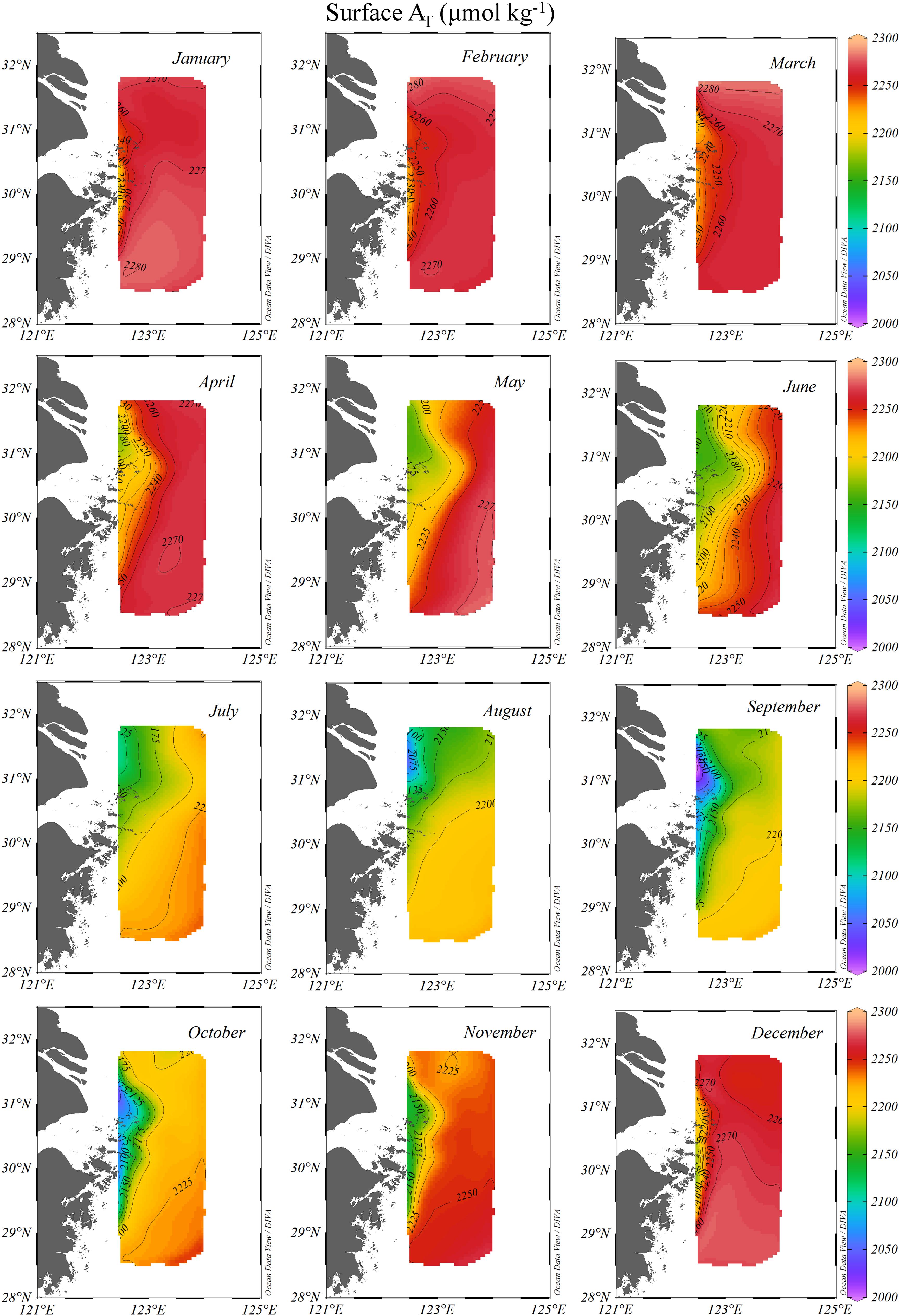
Figure 8. Spatial distribution of monthly average surface ANN-derived total alkalinity using Changjiang Biology FVCOM Data on the ECS shelf from 2000 to 2016.

During the wet season (May to October), A_T values show a wide range, from ∼2000 to ∼2270 μmol kg^–1, water of lower A_T is confined mainly to the northwestern part of the study area, near Changjiang Estuary, whereas water of higher A_T is found in the southeastern part of the study area. Concentrations generally increase moving eastward from the coast to the shelf break, and strongly reflect the summer circulation pattern. Water with low A_T in the northwestern part of the study area is indicative of CDW, spreading eastwards under the influence of the southwest monsoon and characterized by low salinity during the wet season. Water with higher A_T in the southeastern of the study area is strongly influenced by the TWC, which flows into the ECS shelf from the Taiwan Strait.

To assess the approach of combining the ANN model with the Changjiang Biology FVCOM Data to estimate A_T on the ECS shelf, we compared retrieved A_T using the Changjiang Biology FVCOM Data with retrieved A_T using in situ measured T, S, and DO, and also published A_T values (Table 2 and Figure 9). Overall the agreement is good here and supports the reliability of the ANN model on the ECS shelf.

TABLE 2

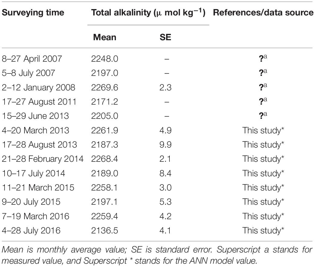
Table 2. Summary information of surface total alkalinity on the East China Sea shelf from 2007 to 2016.

FIGURE 9

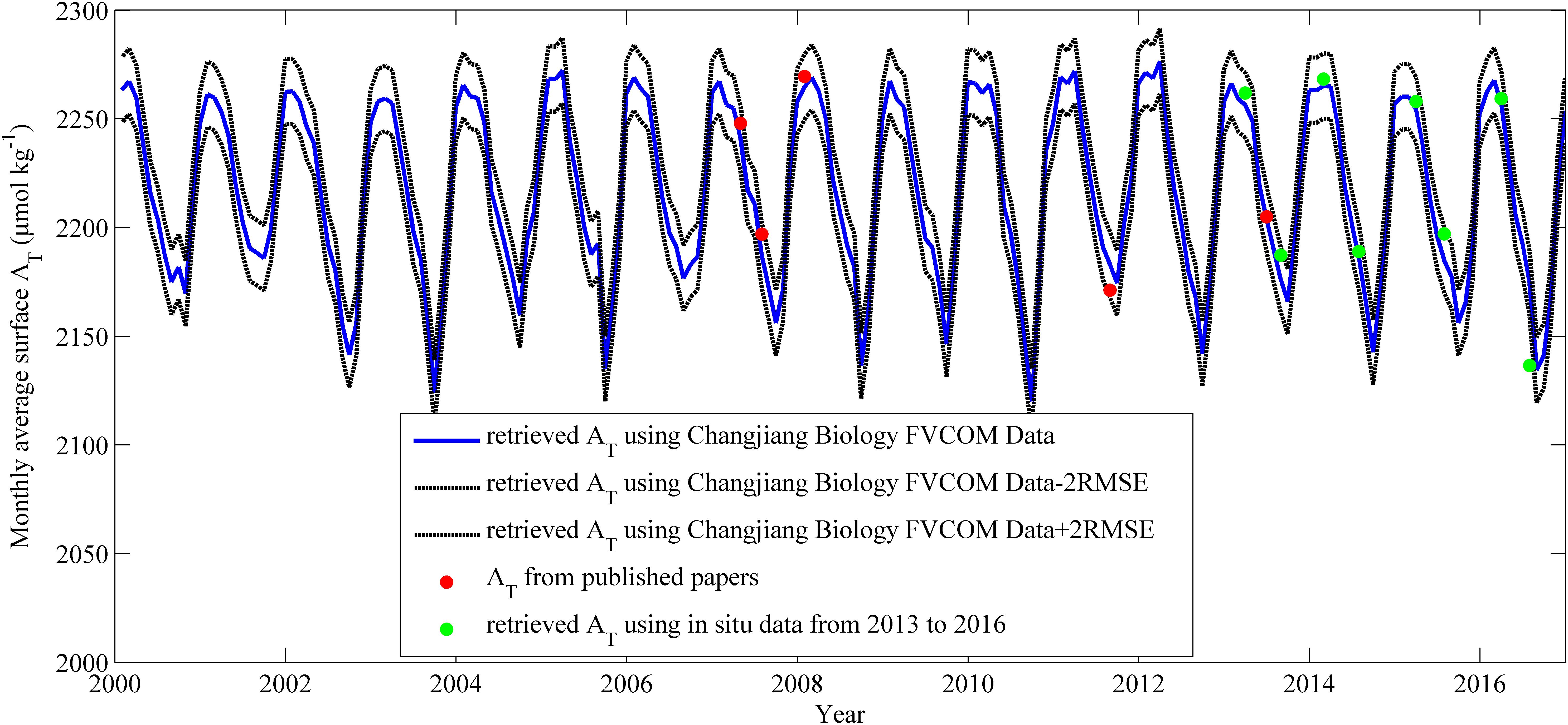
Figure 9. Comparison of monthly average surface total alkalinity on the ECS shelf [(122–124°E;28.5–32.5°N)]. Blue solid line represents retrieved A_T using Changjiang Biology FVCOM Data; black dotted line represents retrieved A_T using Changjiang Biology FVCOM Data ±2RMSE; red point represents mearsured A_T from published papers (e.g., Chou et al., 2009, 2011; Zhai et al., 2014a; Qu et al., 2015, 2017); green point represents retrieved A_T using in situ data from 2013 to 2016.

Seasonality of Total Alkalinity Retrieved From FVCOM Output

Seasonal cycles of surface, middle and bottom layer T and S from FVCOM Data and ANN-derived A_T were calculated for the ECS shelf from 2000 to 2016 (Figure 10). The cycles of A_T and S in the middle and bottom layers are consistent (Figures 10B,C), gradually decreasing from March to September then slowly increasing from September to December, after reaching minimum values in September. This reflects the strong positive correlations between A_T and S in the middle and bottom layer. In the surface layer, seasonal salinity variations strongly reflect freshening due to Changjiang River discharge (Supplementary Figure S2). However, the seasonal cycle of retrieved A_T is lagged by 2 months relative to the salinity cycle, reaching its minimum in September rather than July (Figure 10C). It seems strongly weighted by the period between July and October, when no data were available to train the neuronal network. In order to get more accurate results, training cruises that cover well enough the seasonal cycle are needed.

FIGURE 10

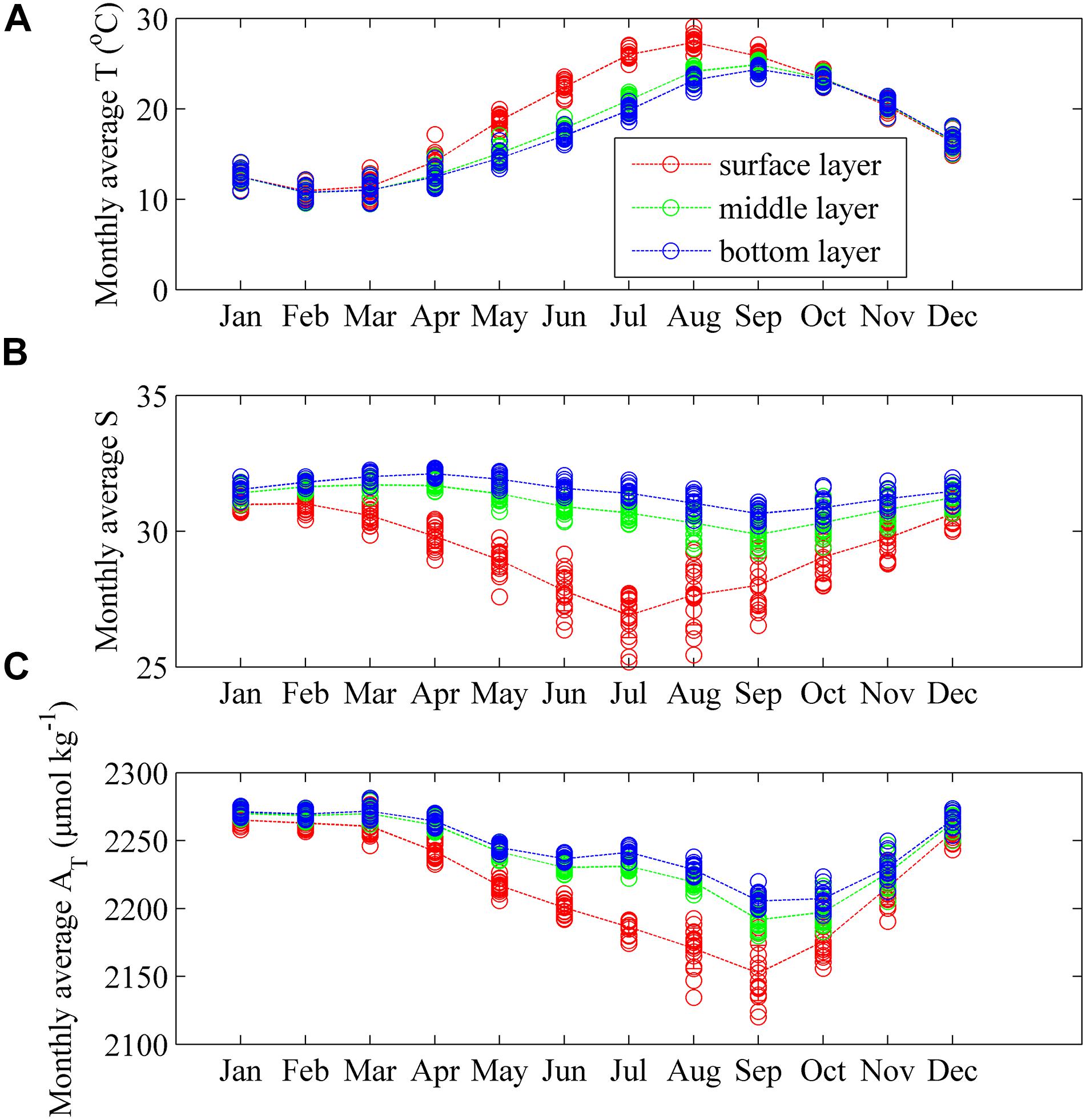
Figure 10. Seasonal cycles of surface, middle and bottom layer parameters T, S, and A_T on the ECS shelf from 2000 to 2016. (A)-temperature; (B)-salinity; (C)-ANN-derived total alkalinity. Red, green, and blue circles show surface, middle, and bottom layers, respectively.

The surface, middle and bottom A_T displays its maximum in January and minimum in September, and the A_T values vary seasonally by up to ∼112 μmol kg^–1 in the surface layer, up to ∼78 μmol kg^–1 in the middle layer, and up to ∼66 μmol kg^–1 in the bottom layer. This is an order of magnitude higher than the open ocean A_T variation estimated by Lee et al. (2006).

Correlations and Seasonal Amplitudes of Surface Total Alkalinity and Salinity Cycles

The retrieved surface A_T distribution appears to reflect mixing between different water masses during the dry and wet seasons. During the dry season (November to April of the next year), S and A_T values vary within a relatively narrow range from 21 to 34 and from 2130 to 2290 μmol kg^–1, respectively, while during the wet season (May to October), S and A_T values vary within a relatively wide range from 15 to 34 and from 2000 to 2270 μmol kg^–1, respectively. To further understand the correlations between surface A_T and S, monthly A_T-S diagrams (Figure 11) were created.

FIGURE 11

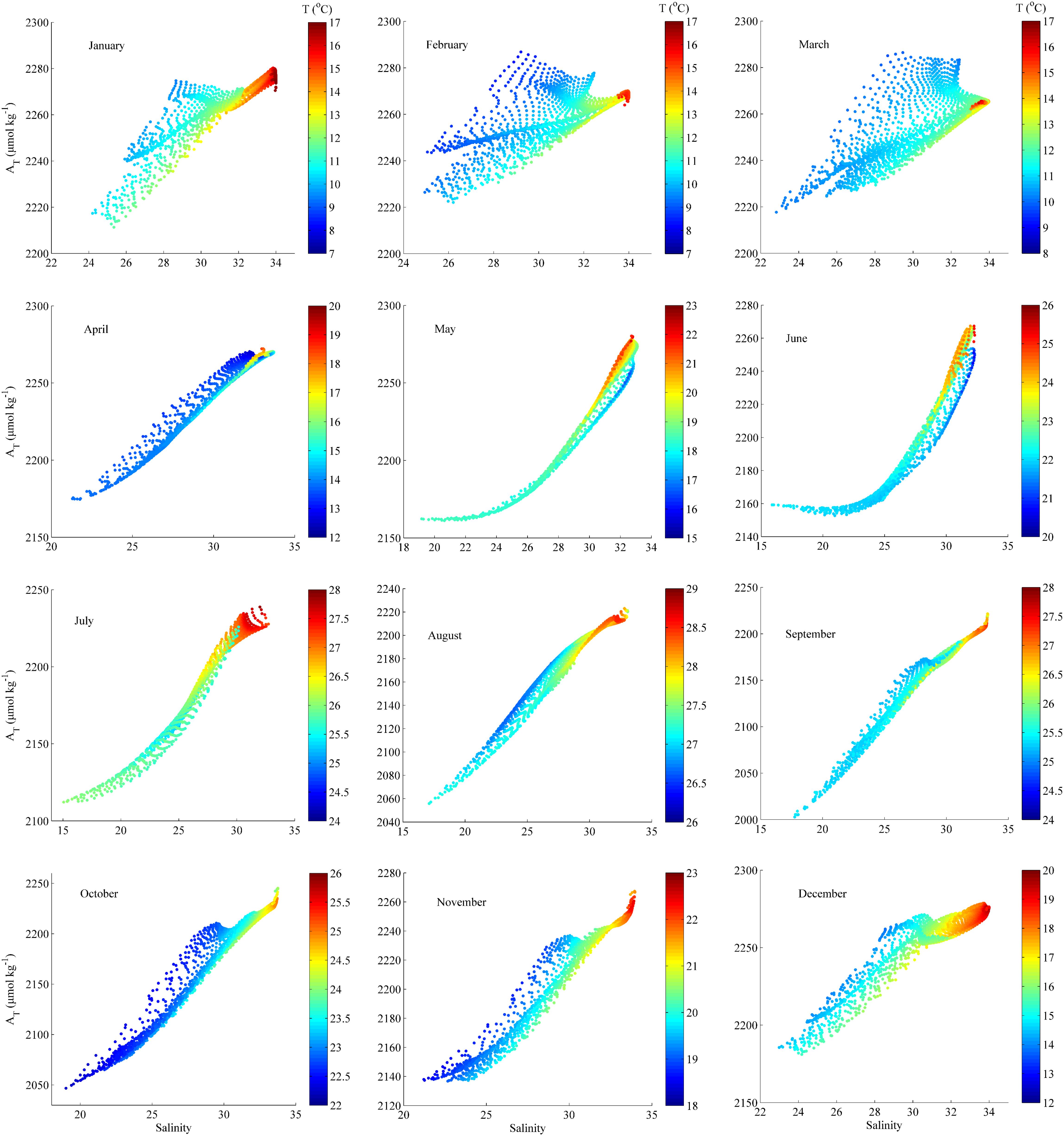
Figure 11. Relationships between monthly surface salinity and ANN-derived total alkalinity on the ECS shelf from 2000 to 2016. The color bar represents temperature.

The study region is mainly influenced by three water masses: the Yellow Sea Coastal Water (YSCW), the CDW, and the Taiwan Strait Warm Water (TSWW). YSCW flows into the northern part of the study area under the influence of coastal current (Figure 1B) and is indicated by high A_T (Figure 11), while the CDW spreads eastward during the prevailing southwest monsoon (Figure 1B), characterized by the lowest S and A_T (Figure 11). The remaining TSWW flows into the ECS through the Taiwan Strait (Figure 1B), characterized by relatively high S and A_T. Monthly linear slopes and intercepts between A_T and S were fitted by Matlab cftool (R2013b) using the robust least-squares fitting method (Table 3). There are seasonally distinct slopes and the intercepts, with smaller slopes from 3.46 to 9.18 and higher intercepts from 1964 to 2126 μmol kg^–1 during the dry season and greater slopes from 10.22 to 14.47 and lower intercepts from 1749 to 1913 μmol kg^–1 during the wet season. This difference may be mainly attributed to strong YSCW and weak CDW during the dry season and strong CDW during the wet season.

TABLE 3

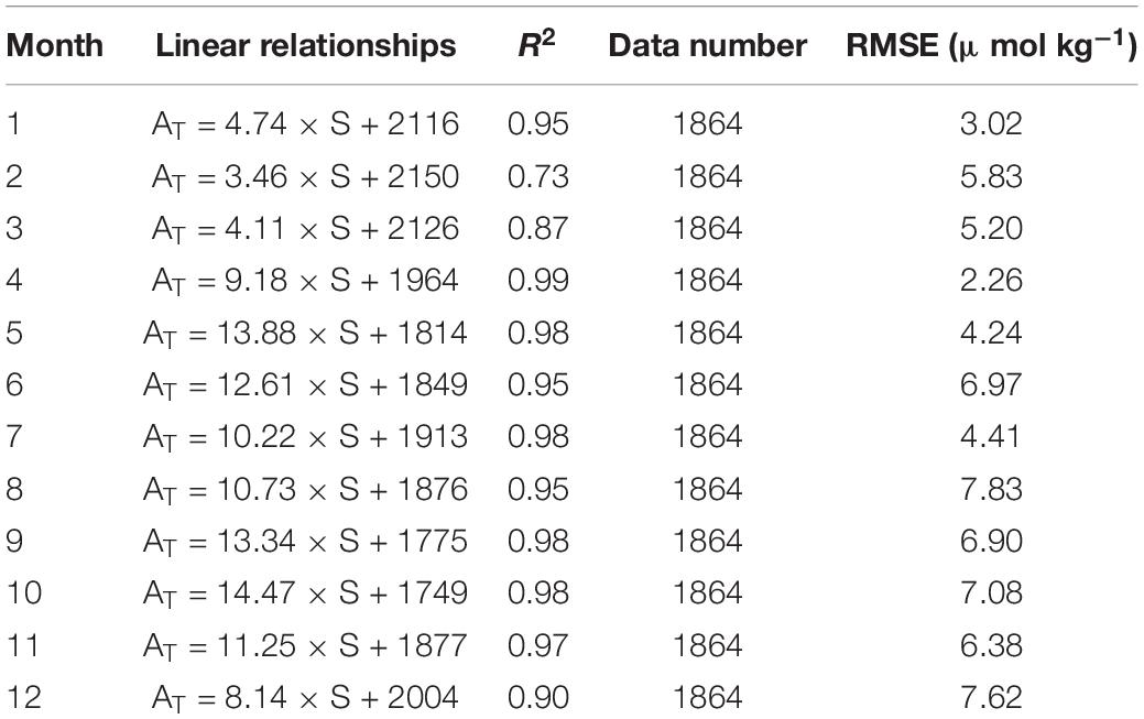
Table 3. Monthly linear relationships (with 95% confidence bounds) between surface total alkalinity and salinity in the study area.

The magnitude of the seasonal variability of surface A_T, computed by differencing the maximum and minimum monthly mean A_T values in each grid point, has a spatial pattern that is similar though not identical to that of the magnitude of seasonal salinity variability (Figure 12). The largest seasonal fluctuations of surface A_T and salinity are found on the inner shelf near the Changjiang Estuary, which is under the influence of the Changjiang River discharge. In contrast, A_T in the southeastern part of the study area exhibits a very weak seasonality.

FIGURE 12

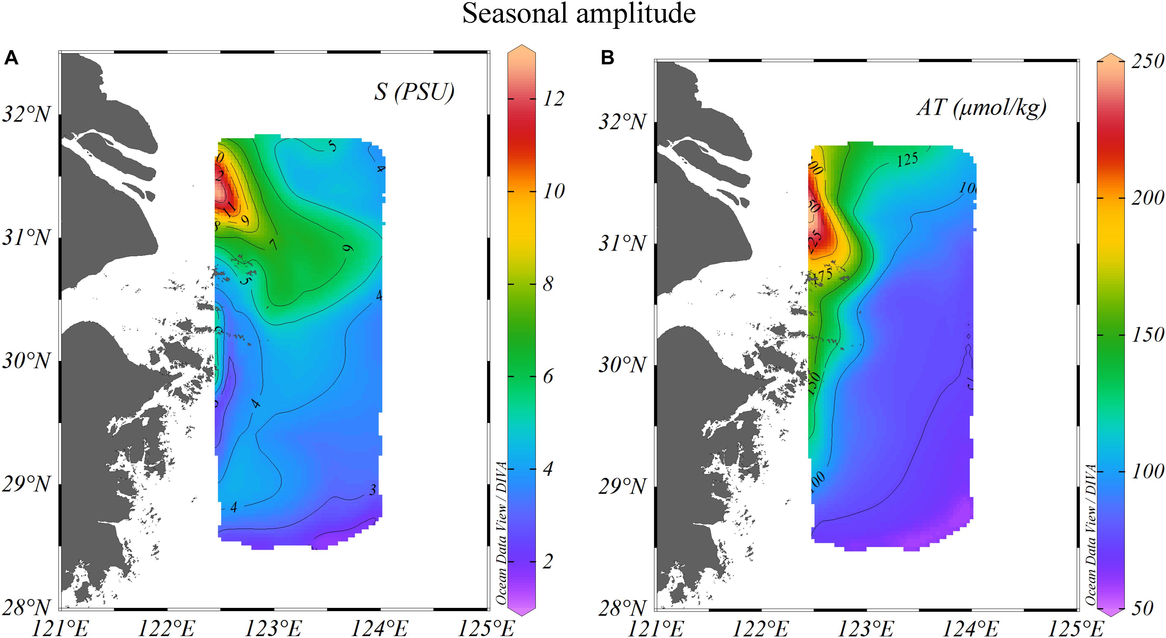
Figure 12. Distribution of the seasonal amplitude (maximum minus minimum) of surface ANN-derived total alkalinity and salinity on the ECS shelf from 2000 to 2016. (A)-salinity; (B)-ANN-derived total alkalinity.

Conclusion and Perspectives

We have developed an ANN model, and used it to calculate surface A_T for eight cruises during 2013–2016, and to retrieve monthly A_T for the period 2000–2016 on the East China Sea shelf. The two most important predictor variables were salinity and longitude, and seasonal variations in retrieved A_T could be mainly attributed to the seasonal cycle of the Changjiang River discharge on the East China Sea shelf.

The model has several potential applications. For example, it can provide estimates of seawater A_T with known accuracies for the East China Sea shelf. Within this region the model could be used as a cost-effective way to overcome restrictions of limited marine observations conducted from ships, such as coarse resolution and under-sampling of carbonate system variables, and may be a valuable tool for understanding the seasonal variation of A_T in poorly observed regions. This approach can also be applied to other regions to estimate A_T by suitably adapting the input variables and network structure. In order to get more accurate seasonal trend, training cruises that cover well enough the seasonal cycle are needed.

Data Availability Statement

Matlab code of the ANN model for A_T estimation and five cruises data used from 2008 to 2018 are available http://doi.org/10.5281/zenodo.3491486, including one cruise data during 2008 downloaded from https://www.nodc.noaa.gov/ocads/oceans/RepeatSections/clivar_ORI_885.html.

Requests to access the raw data should be directed to RB: Richard.Bellerby@niva.no.

The input variables from the Changjiang Biology Finite-Volume Coastal Ocean Model (FVCOM) Data were first downloaded from http://47.101.49.44/wms/demo, then monthly input variables (T, S, DO) and retrieved total alkalinity from 2000 to 2016 and retrieved surface total alkalinity of eight cruises from 2013 to 2016 on the East China Sea shelf are available: http://doi.org/10.5281/zenodo.3406551.

Distributions and seasonal amplitudes of surface total alkalinity retrieved from the Changjiang Biology FVCOM Data and Correlations between surface total alkalinity and salinity are available: http://doi.org/10.5281/zenodo.3491996.

Seasonal cycles of surface, middle, and bottom total alkalinity retrieved from the Changjiang Biology FVCOM Data on the ECS shelf from 2000 to 2016 are available: http://doi.org/10.5281/zenodo.3491998.

Comparison between retrieved A_T using the Changjiang Biology FVCOM Data and retrieved A_T using in situ measured T, S, and DO, and also published A_T values are available: http://doi.org/10.5281/zenodo.3492004.

Author Contributions

XL, RB, and PW contributed to the development of the methodology and designed the model. JG provided the input variables from the Changjiang Biology Finite-Volume Coastal Ocean Model (FVCOM) Data and eight cruises data on the East China Sea shelf during 2013–2016. JEL, AY, and JGL provided four cruises dataset from 2017 to 2018 year. XL developed the model code and performed the simulations. All authors contributed to development of the manuscript.

Funding

This study was financially supported by the National Thousand Talents Program for Foreign Experts (Grants No. WQ20133100150), Vulnerabilities and Opportunities of the Coastal Ocean (Grants No. SKLEC-2016RCDW01), Marginal Seas (MARSEAS) (Grants SKLEC-Taskteam project), and Innovative Talents International Cooperation Training Project (Grants No. China Scholarship Council-201913045). RB and PW were also supported by the FRAM High North Research Centre for Climate and the Environment under the Ocean Acidification Flagship and the NIVA Land-Ocean Interactions Strategic Institute program.

Conflict of Interest

The authors declare that the research was conducted in the absence of any commercial or financial relationships that could be construed as a potential conflict of interest.

Acknowledgments

We deeply thank the people who worked on the cruises and in the laboratory and Chou et al. (2011) providing one cruise data from 2 to 9 January 2008 in the ECS.

Supplementary Material

The Supplementary Material for this article can be found online at: https://www.frontiersin.org/articles/10.3389/fmars.2020.00219/full#supplementary-material

Footnotes

1. ^ https://www.nodc.noaa.gov/ocads/oceans/RepeatSections/clivar_ORI_885.html
2. ^ http://47.101.49.44/wms/demo

References

Alin, S. R., Feely, R. A., Dickson, A. G., Hernández-Ayón, J. M., Juranek, L. W., Ohman, M. D., et al. (2012). Robust empirical relationships for estimating the carbonate system in the southern California current system and application to CalCOFI hydrographic cruise data (2005–2011). J. Geophys. Res. Oceans 117:C05033. doi: 10.1029/2011JC007511

CrossRef Full Text | Google Scholar

Borges, A. V., Delille, B., and Frankignoull, M. (2005). Budgeting sinks and sources of CO2 in the coastal ocean: diversity of ecosystems counts. Geophys. Res. Lett. 32:L14601. doi: 10.1029/2005GL023053

CrossRef Full Text | Google Scholar

Bostock, H. C., Mikaloff Fletcher, S. E., and Williams, M. J. M. (2013). Estimating carbonate parameters from hydrographic data for the intermediate and deep waters of the Southern Hemisphere oceans. Biogeosciences 10, 6199–6213.

Google Scholar

Broullón, D., Pérez, F. F., Velo, A., Hoppema, M., Olsen, A., Takahashi, T., et al. (2019). A global monthly climatology of total alkalinity: a neural network approach. Earth Syst. Sci. Data 11, 1109–1127.

Google Scholar

Cai, W. J., Dai, M. H., and Wang, Y. (2006). Air-sea exchange of carbon dioxide in ocean margins: a province-based synthesis. Geophys. Res. Lett. 33:L12603. doi: 10.1029/2006GL026219

CrossRef Full Text | Google Scholar

Cai, W. J., Hu, X. P., Huang, W. J., Murrell, M. C., Lehrter, J. C., Lohrenz, S. E., et al. (2011). Acidification of subsurface coastal waters enhanced by eutrophication. Nat. Geosci. 4, 766–770. doi: 10.1038/NGEO1297

PubMed Abstract | CrossRef Full Text | Google Scholar

Carter, B. R., Feely, R. A., Williams, N. L., Dickson, A. G., Fong, M. B., and Takeshita, Y. (2018). Updated methods for global locally interpolated estimation of alkalinity, pH, and nitrate. Limnol. Oceanogr. Methods 16, 119–131. doi: 10.1002/lom3.10232

CrossRef Full Text | Google Scholar

Carter, B. R., Williams, N. L., Gray, A. R., and Feely, R. A. (2016). Locally interpolated alkalinity regression for global alkalinity estimation. Limnol. Oceanogr. Methods 14, 268–277. doi: 10.1002/lom3.10087

CrossRef Full Text | Google Scholar

Chou, W. C., Gong, G. C., Cai, W. J., and Tseng, C. M. (2013). Seasonality of CO2 in coastal oceans altered by increasing anthropogenic nutrient delivery from large rivers: evidence from the Changjiang–East China Sea system. Biogeosciences 10, 3889–3899.

Google Scholar

Chou, W. C., Gong, G. C., Sheu, D. D., Hung, C. C., and Tseng, T. F. (2009). Surface distributions of carbon chemistry parameters in the East China Sea in summer 2007. J. Geophys. Res. 114:C07026. doi: 10.1029/2008JC005128

CrossRef Full Text | Google Scholar

Chou, W. C., Gong, G. C., Tseng, C. M., Sheu, D. D., Hung, C. C., Chang, L. P., et al. (2011). The carbonate system in the East China Sea in winter: a eutrophication-induced seasonal shift in CO2 uptake. Mar. Chem. 123, 44–55. doi: 10.1016/j.marchem.2010.09.004

CrossRef Full Text | Google Scholar

Dickson, A. G., Sabine, C. L., and Christian, J. R. (2007). Guide to Best Practices for Ocean CO2 Measurements: (PICES Special Publication 3; IOCCP Report 8). Sidney, BC: North Pacific Marine Science Organization, 191.

Google Scholar

Doney, S. C., Mahowald, N., Lima, I., Feely, R. A., Mackenzie, F. T., Lamarque, J. F., et al. (2007). Impact of anthropogenic atmospheric nitrogen and sulfur deposition on ocean acidification and the inorganic carbon system. Proc. Natl. Acad. Sci. U.S.A. 104, 14580–14585. doi: 10.1073/pnas.0702218104

PubMed Abstract | CrossRef Full Text | Google Scholar

Evans, W., Mathis, J. T., Winsor, P., Statscewich, H., and Whitledge, T. E. (2013). A regression modeling approach for studying carbonate system variability in the northern Gulf of Alaska. J. Geophys. Res. Oceans 118, 476–489. doi: 10.1029/2012JC008246

CrossRef Full Text | Google Scholar

Fassbender, A. J., Alin, S. R., Feely, R. A., Sutton, A. J., Newton, J. A., and Byrne, R. H. (2017). Estimating total alkalinity in the Washington State coastal zone: complexities and surprising utility for ocean acidification research. Estuaries Coasts 40, 404–418. doi: 10.1007/s12237-016-0168-z

CrossRef Full Text | Google Scholar

Fine, R. A., Willey, D. A., and Millero, F. J. (2017). Global variability and changes in ocean total alkalinity from Aquarius satellite data. Geophys. Res. Lett. 44, 261–267. doi: 10.1002/2016GL071712

CrossRef Full Text | Google Scholar

Friedrich, T., and Oschlies, A. (2009). Neural network-based estimates of North Atlantic surface pCO2 from satellite data: a methodological study. J. Geophys. Res. 114:C03020. doi: 10.1029/2007JC004646

CrossRef Full Text | Google Scholar

Friis, K., Körtzinger, A., and Wallace, D. W. R. (2003). The salinity normalization of marine inorganic carbon chemistry data. Geophys. Res. Lett. 30:1085. doi: 10.1029/2002GL015898

CrossRef Full Text | Google Scholar

Gattuso, J. P., Frankignoulle, M., and Wollast, R. (1998). Carbon and carbonate metabolism in coastal aquatic ecosystems. Annu. Rev. Ecol. Syst. 29, 405–434. doi: 10.1146/annurev.ecolsys.29.1.405

CrossRef Full Text | Google Scholar

Gemayel, E., Hassoun, A. E. R., Benallal, M. A., Goyet, C., Rivaro, P., Saab, M. A. A., et al. (2015). Climatological variations of total alkalinity and total dissolved inorganic carbon in the Mediterranean Sea surface waters. Earth Syst. Dyn. 6, 789–800.

Google Scholar

Gong, G. C., Chen, Y. L. L., and Liu, K. K. (1996). Chemical hydrography and chlorophyll a distribution in the East China Sea in summer: implications in nutrient dynamics. Cont. Shelf Res. 16, 1561–1590.

Google Scholar

Guo, X. H., Zhai, W. D., Dai, M. H., Zhang, C., Bai, Y., Xu, Y., et al. (2015). Air–sea CO2 fluxes in the East China Sea based on multiple-year underway observations. Biogeosciences 12, 5495–5514.

Google Scholar

Hornik, K., Stinchcombe, M., and White, H. (1989). Multilayer feedforward networks are universal approximators. Neural Netw. 2, 359–366.

Google Scholar

Hur, H. B., Jacobs, G. A., and Teague, W. J. (1999). Monthly variations of water masses in the Yellow and East China Seas. J. Oceanogr. 55, 171–184.

Google Scholar

Juranek, L. W., Feely, R. A., Peterson, W. T., Alin, S. R., Hales, B., Lee, K., et al. (2009). A novel method for determination of aragonite saturation state on the continental shelf of central Oregon using multi-parameter relationships with hydrographic data. Geophys. Res. Lett. 36:L24601. doi: 10.1029/2009GL040778

CrossRef Full Text | Google Scholar

Kim, T.-W., Lee, K., Feely, R. A., Sabine, C. L., Chen, C.-T. A., Jeong, H. J., et al. (2010). Prediction of Sea of Japan (East Sea) acidification over the past 40 years using a multiparameter regression model. Global Biogeochem. Cycles 24:GB3005. doi: 10.1029/2009GB003637

CrossRef Full Text | Google Scholar

Laruelle, G. G., Landschützer, P., Gruber, N., Tison, J. L., Delille, B., and Regnier, P. (2017). Global high-resolution monthly pCO2 climatology for the coastal ocean derived from neural network interpolation. Biogeosciences 14, 4545–4561.

Google Scholar

Lee, H. J., and Chao, S. Y. (2003). A climatological description of circulation in and around the East China Sea. Deep Sea Res. Part II Top. Stud. Oceanogr. 50, 1065–1084.

Google Scholar

Lee, K., Tong, L. T., Millero, F. J., Sabine, C. L., Dickson, A. G., Goyet, C., et al. (2006). Global relationships of total alkalinity with salinity and temperature in surface waters of the world’s oceans. Geophys. Res. Lett. 33:L19605. doi: 10.1029/2006GL027207

CrossRef Full Text | Google Scholar

Li, G. X., Han, X. B., Yue, S. H., Wen, G. Y., Yang, R. M., and Kusky, T. M. (2006). Monthly variations of water masses in the East China Seas. Cont. Shelf Res. 26, 1954–1970.

Google Scholar

Luo, X. F., Wei, H., Liu, Z., and Zhao, L. (2015). Seasonal variability of air–sea CO2 fluxes in the Yellow and East China Seas: a case study of continental shelf sea carbon cycle model. Cont. Shelf Res. 107, 69–78. doi: 10.1016/j.csr.2015.07.009

CrossRef Full Text | Google Scholar

Millero, F. J. (2007). The marine inorganic carbon cycle. Chem. Rev. 107, 308–341. doi: 10.1021/cr0503557

CrossRef Full Text | Google Scholar

Millero, F. J., Lee, K., and Roche, M. (1998). Distribution of alkalinity in the surface waters of the major oceans. Mar. Chem. 60, 111–130.

Google Scholar

Mintrop, L., Pérez, F. F., González Dávila, M., Santana-Casiano, J. M., and Körtzinger, A. (2000). Alkalinity determination by potentiometry: intercalibration using three different methods. Ciencias Marinas 26, 23–37. doi: 10.7773/cm.v26i1.573

CrossRef Full Text | Google Scholar

Olden, J. D., and Jackson, D. A. (2002). Illuminating the “black box”: a randomization approach for understanding variable contributions in artificial neural networks. Ecol. Modell. 154, 135–150.

Google Scholar

Olden, J. D., Joy, M. K., and Death, R. G. (2004). An accurate comparison of methods for quantifying variable importance in artificial neural networks using simulated data. Ecol. Modell. 178, 389–397. doi: 10.1016/j.ecolmodel.2004.03.013

CrossRef Full Text | Google Scholar

Omar, A. M., Thomas, H., Olsen, A., Becker, M., Skjelvan, I., and Reverdin, G. (2019). Trends of Ocean acidification and pCO2 in the northern North Sea, 2003–2015. J. Geophys. Res. Biogeosci. 124, 3088–3103. doi: 10.1029/2018JG004992

CrossRef Full Text | Google Scholar

Qu, B. X., Song, J. M., Yuan, H. M., Li, X. G., Li, N., and Duan, L. Q. (2017). Comparison of carbonate parameters and air–sea CO2 flux in the southern Yellow Sea and East China Sea during spring and summer of 2011. J. Oceanogr. 73, 365–382.

Google Scholar

Qu, B. X., Song, J. M., Yuan, H. M., Li, X. G., Li, N., Duan, L. Q., et al. (2015). Summer carbonate chemistry dynamics in the Southern Yellow Sea and the East China Sea: regional variations and controls. Cont. Shelf Res. 111, 250–261. doi: 10.1016/j.csr.2015.08.017

CrossRef Full Text | Google Scholar

Raitsos, D. E., Lavender, S. J., Maravelias, C. D., Haralabous, J., Richardson, A. J., and Reid, P. C. (2008). Identifying four phytoplankton functional types from space: an ecological approach. Limnol. Oceanogr. 53, 605–613. doi: 10.4319/lo.2008.53.2.0605

CrossRef Full Text | Google Scholar

Sasse, T. P., McNeil, B. I., and Abramowitz, G. (2013). A novel method for diagnosing seasonal to inter-annual surface ocean carbon dynamics from bottle data using neural networks. Biogeosciences 10, 4319–4340.

Google Scholar

Sauzède, R., Bittig, H. C., Claustre, H., de Fommervault, O. P., Gattuso, J. P., Legendre, L., et al. (2017). Estimates of water-column nutrient concentrations and carbonate system parameters in the global Ocean: a novel approach based on neural networks. Front. Mar. Sci. 4:128. doi: 10.3389/fmars.2017.00128

CrossRef Full Text | Google Scholar

Sauzède, R., Claustre, H., Jamet, C., Uitz, J., Ras, J., Mignot, A., et al. (2015). Retrieving the vertical distribution of chlorophyll-a concentration and phytoplankton community composition from in situ fluorescence profiles: a method based on a neural network with potential for global-scale applications. J. Geophys. Res. Oceans 120, 451–470. doi: 10.1002/2014JC010355

CrossRef Full Text | Google Scholar

Sauzède, R., Claustre, H., Uitz, J., Jamet, C., Dall’Olmo, G., D’Ortenzio, F., et al. (2016). A neural network-based method for merging ocean color and Argo data to extend surface bio-optical properties to depth: retrieval of the particulate backscattering coefficient. J. Geophys. Res. Oceans 121, 2552–2571. doi: 10.1002/2015JC011408

CrossRef Full Text | Google Scholar

Shim, J. H., Kim, D., Kang, Y. C., Lee, J. H., Jang, S. T., and Kim, C. H. (2007). Seasonal variations in pCO2 and its controlling factors in surface seawater of the northern East China Sea. Cont. Shelf Res. 27, 2623–2636. doi: 10.1016/j.csr.2007.07.005

CrossRef Full Text | Google Scholar

Tamura, S., and Tateishi, M. (1997). Capabilities of a four-layered feedforward neural network: four layers versus three. IEEE Trans. Neural Netw. 8, 251–255. doi: 10.1109/72.557662

PubMed Abstract | CrossRef Full Text | Google Scholar

Uusitalo, L. (2007). Advantages and challenges of Bayesian networks in environmental modelling. Ecol. Modell. 203, 312–318. doi: 10.1016/j.ecolmodel.2006.11.033

CrossRef Full Text | Google Scholar

Velo, A., Pérez, F. F., Tanhua, T., Gilcoto, M., Ríos, A. F., and Key, R. M. (2013). Total alkalinity estimation using MLR and neural network techniques. J. Mar. Syst. 11, 11–18. doi: 10.1016/j.jmarsys.2012.09.002

CrossRef Full Text | Google Scholar

Zhai, W. D., Chen, J. F., Jin, H. Y., Li, H. L., Liu, J. W., He, X. Q., et al. (2014a). Spring carbonate chemistry dynamics of surface waters in the northern East China Sea: water mixing, biological uptake of CO2, and chemical buffering capacity. J. Geophys. Res. Oceans 119, 5638–5653. doi: 10.1002/2014JC009856

CrossRef Full Text | Google Scholar

Zhai, W. D., and Dai, M. H. (2009). On the seasonal variation of air-sea CO2 fluxes in the outer Changjiang (Yangtze River) Estuary, East China Sea. Mar. Chem. 117, 2–10. doi: 10.1016/j.marchem.2009.02.008

CrossRef Full Text | Google Scholar

Zhai, W. D., Zheng, N., Huo, C., Xu, Y., Zhao, H. D., Li, Y. W., et al. (2014b). Subsurface pH and carbonate saturation state of aragonite on the Chinese side of the North Yellow Sea: seasonal variations and controls. Biogeosciences 11, 1103–1123. doi: 10.5194/bg-11-1103-2014

CrossRef Full Text | Google Scholar