Classification and Mapping of Benthic Biotopes in Arctic and Sub-Arctic Norwegian Waters

Introduction

An increasing interest in deep-sea resources has brought about a growing number of offshore activities such as industrial fishing, mining, and oil and gas extraction (Ramirez Llodra et al., 2011). These activities cause a wide range of pressures on benthic ecosystems including animal removal, habitat destruction, sedimentation, pollution, etc. The ecological effects of these pressures (i.e., impacts) may include local and global species extinctions, altered food web dynamics, loss of connectivity, decreased ecosystem stability, and altered patterns of biogeochemical cycling (McCauley, 2015). Area-based management is a tool to avoid negative impact on biological communities, habitats, and the environment. In addition, ongoing climate change heightens the need for solid knowledge of marine ecosystems to support appropriate management strategies. Area-based management, however, typically requires spatial ecological data, which is notably difficult to obtain (Steltzenmüller et al., 2013).

The Marine AREAl database for NOrwegian waters (MAREANO) program conducts seabed mapping, as required by the Norwegian government, in order to fill knowledge gaps relevant to the implementation of management plans for different parts of the Norwegian EEZ. The program was launched in 2005 with the goal of obtaining information that can be used as a scientific basis for the regulation of human activities such as those undertaken by the petroleum industry and fisheries. By using a variety of complementary sampling gears (such as towed video, beam trawl, Van Veen grab, and Rothlisberg and Pearcy sledge) to ensure that a broad set of benthic organisms on all types of seabed are represented, MAREANO offers a unique insight into the diversity, biomass, and production of benthic communities. Map products and data from MAREANO include bathymetric and geological maps as well as information on environmental status, species distribution, biological production, biodiversity, habitats, and biotopes. The latter being the focus of this paper.

In this paper, we utilize video data (results from analyses of video records) to define and predict benthic biotopes. Although video observations are mainly documenting epi-benthic megafauna (>c. 5 cm), they provide information on community composition from all substrate types. These observations are therefore useful for characterizing biotopes from a wider range of seabed substrates than is possible with physical sampling tools. By combining the MAREANO data and map products with modeled oceanographic data (temperature, salinity, and currents near the sea floor), the ecological insights that can be gained from the MAREANO data are enhanced.

A biotope can be defined as a combined characteristic species composition and environmental settings. In particular, the physical characteristics of water masses near the seabed, topography, and seabed substrate are often the main determining factors (Barnes and Hughes, 1982; Harris, 2012; in review) shaping benthic communities. These environmental settings can be used to predict biotope distribution in areas without observations using methods common to habitat distribution modeling (HDM).

Biotope maps can display multiple biotopes simultaneously, suggesting the most likely biotope to occur in each area (as shown in this study), or they can display the probability of occurrence of a single biotope, similar to a species distribution model (e.g., Ross and Howell, 2013). The multi-biotope format is better suited for assessing the likely distribution of the biotopes we define in this study compared to a set of individual single biotope maps. Both map types are generated by MAREANO, where the single biotope maps are used for vulnerable marine ecosystems. In this paper, we focus on the identification of biotopes and environmental factors that correlate with their spatial distribution. The aim of this study is: (1) classification of biotopes based on megafaunal composition at observed seabed areas and (2) to relate these biotopes to environmental variables that can be used to predict the distribution of biotopes across the entire mapping area.

Materials and Methods

The study area was surveyed over the course of 12 years (2006–2018) collecting video transects at 757 different locations (none of which were repeat visits) within the Norwegian Barents Sea region including shelf areas off Troms and Finnmark counties and north-eastern shelf and slope areas in the Norwegian Sea (Figure 1). This area comprises a wide range of environmental conditions over which we know there is a varied distribution of benthic communities. The continental margin offshore North Norway described here is in the area 68°N–77°N and 15°E–37°E.

FIGURE 1

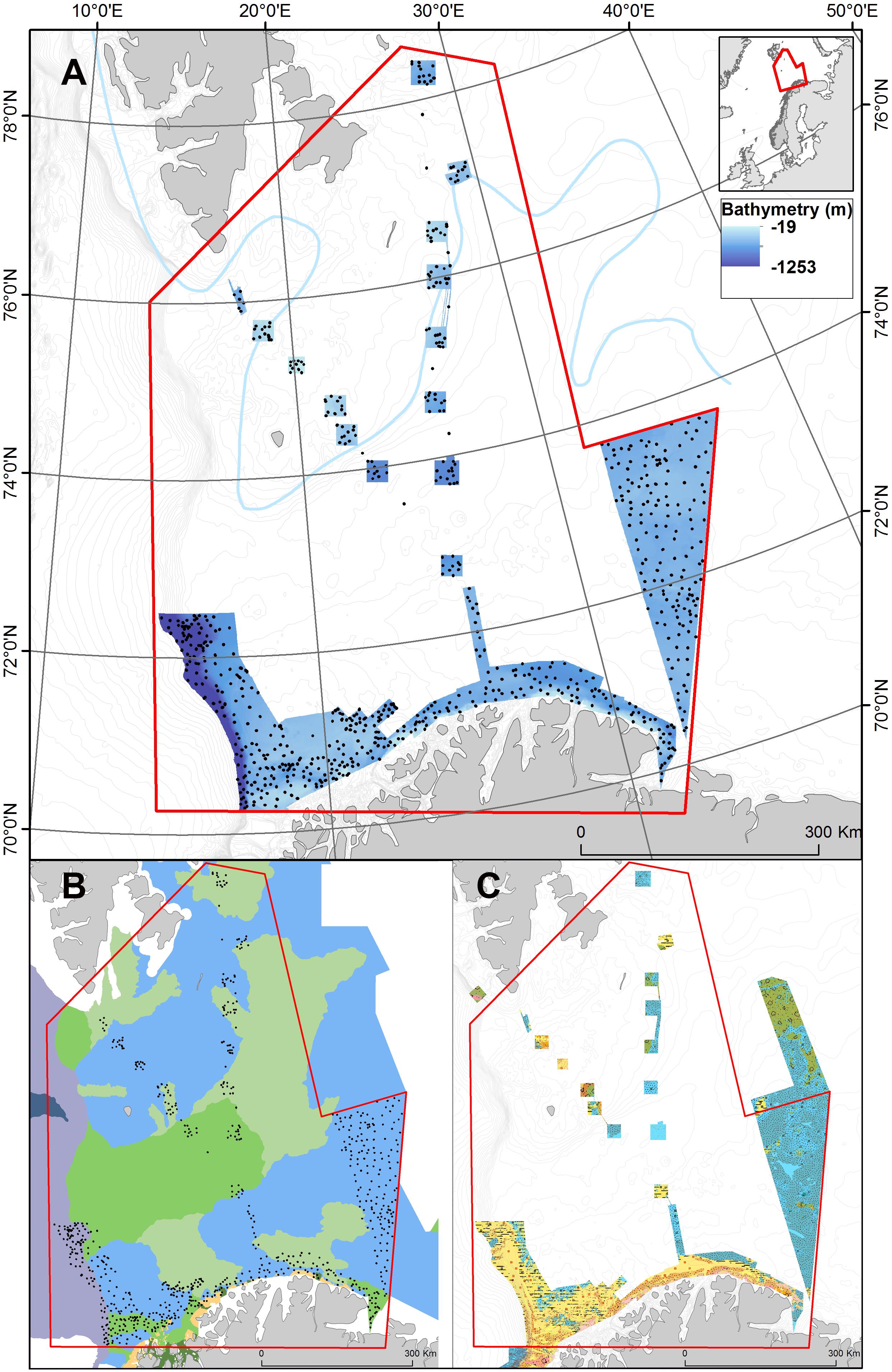
Figure 1. (A) Map of the study area in the Barents Sea. The extent of the study area is indicated in red and MAREANO video stations used in this study area shown as black dots over color shaded bathymetry from Kartverket https://mareano.no/en/maps-and-data/marine-geospatial-data. The approximate location of the polar front is indicated with a line. (B) A MAREANO landscape map (broad-scale geomorphology) showing how the area is dominated by continental shelf plain (blue), marine valleys (green), and shallow marine valleys (light green) with areas near the coast comprising strandflat (orange) while deeper areas to the west are classified as smooth continental slope (purple). Full symbology is available at https://www.ngu.no/Mareano/Landscape.html. Landscape mapping procedures are based on Elvenes (2013). (C) A MAREANO sediment map showing how the southwestern part of the study area is dominated by sandy and gravelly sediments (yellow, orange) while eastern areas are dominated by muddy sediments (blue). Full symbology available at https://www.ngu.no/Mareano/Grainsize.html.

Geological Setting

The Barents Sea is a shallow (<800 m deep) epicontinental sea. Depths within the study area range from 24 to 1170 m in the Norwegian Sea and to the full depth of the Barents Sea. The seabed in the study area consists mainly of sedimentary rocks from the Mesozoic and Cenozoic (Sigmond, 2002).

The broad-scale seafloor morphology is a result of repeated glaciations throughout the Quaternary (Knies et al., 2009) and is characterized by a landscape of shallow banks, approximately 20–300 m deep, intersected by deeper marine valleys or troughs, approximately 300–800 m deep (Figure 1B). The seafloor is covered with sediments deposited either sub-glacially or in a glacimarine environment. The type, distribution, and thickness of the majority of unlithified sediments in the study area are a result of glacial and oceanographic processes during the late Pleistocene and Early Holocene, rather than contemporary processes (e.g., Elverhøi et al., 1993; Bjarnadóttir et al., 2014). Similarly, most of the fine-scale seafloor geomorphic features record processes related to the last deglaciation of the area (e.g., Bjarnadóttir et al., 2014), although some areas have since been reshaped by oceanographic processes (e.g., Bellec et al., 2019). Geomorphic features from broad-scale landscapes (Figure 1B) to smaller landforms have been widely documented to be linked to benthic habitat (Harris and Baker, 2011). The modern-day distribution of substrate types (Figure 1C) is influenced by bottom currents, and both are expected to have an important effect on the distribution of benthic fauna. The southwestern part of the study area is dominated by sandy and gravelly sediments, while eastern areas are dominated by muddy sediments (Figure 1C).

Oceanographic Setting

Four major water masses originating in the Atlantic and Arctic oceans meet in the Norwegian Sea (Hansen and Østerhus, 2000), and the associated currents are of fundamental importance for the global climate. The warm, salty North Atlantic Current (NAC) flows in from the Atlantic Ocean, and the colder and less saline Norwegian Coastal Current (NCC) originates in the North Sea. The Norwegian Atlantic water (NAW) extends down to about 500–600 m and is part of the relatively warm and saline NAC. Below this depth, two cold water masses occur: the Norwegian Sea Arctic Intermediate Water (NSAIW) which flows as a continuation of the East Iceland Current from the Iceland and Greenland Seas and the Norwegian Sea Deep Water (NSDW) from the Greenland Sea. NSAIW has a temperature range between −0.5 and 0.5°C, whereas the NSDW typically shows a temperature range between −0.5 and −1.1°C. The interface between these two water masses typically occurs at around 1300 m off the Norwegian coast in the Norwegian Sea (Blindheim, 1990).

The bottom topography with banks and basins steers the currents and influences the distribution of water masses in the Barents Sea (Loeng, 1991). The Norwegian Atlantic Current splits into two main branches, one flowing into and through the Barents Sea from southwest to northeast, the other flowing around the western and northern flanks of the Barents Sea as the West Spitsbergen Current (Skagseth, 2008; Ingvaldsen and Loeng, 2009; Ozhigin et al., 2011). Cold fresh Arctic waters arrive from the Arctic Ocean, entering the Barents Sea between Nordaustlandet and Franz Josef Land and between Franz Josef Land and Novaya Zemlya. The Polar Front is a prominent feature in the Barents Sea, and it represents the transition zone between the warm and saline Atlantic Water and the cold and less saline Arctic and Polar waters.

Video Recording and Annotation

The seabed was inspected using the towed video platforms, “CAMPOD” (as described in Buhl-Mortensen et al., 2009, 2012) and “Chimaera” (as described in Buhl-Mortensen and Buhl-Mortensen, 2017) equipped with similar High-Definition video cameras systems, tilted forward at an angle of approximately 45°. Video was continuously recorded to harddrive along each transect. The video platform was towed behind the survey vessel at a speed of 0.7 knots and controlled by a winch operator providing a near-constant altitude of 1.5 m above the seabed. Each video transect was planned to cover a distance of 700 m, but in practice, the distance varied between 600 and 800 m. Positioning of the video data is provided by a hydroacoustic positioning system (Simrad HIPAP and Eiva Navipac software) with a transponder mounted on the video platform, giving a position accurate to 2% of water depth. Navigational data (date, UTC time, positions, and depth) are recorded automatically at 10-s intervals using the software CampodLogger developed by the Institute of Marine Research (as described in Buhl-Mortensen et al., 2015a, b).

After the cruise a detailed video analysis was undertaken using a custom-made (Institute of Marine Research) software: VideoNavigator (as described in Gomes Pereira et al., 2016). The output of this software is a text file showing time stamped species names, abundances, substrates, comments, field of view (as measured based on laser points mounted 10 cm apart), and image quality records. These biological annotations were then georeferenced by synchronizing the video timestamps with the navigation data which had undergone cleaning to remove spurious pings. X and Y coordinates were recorded in UTM zone 33 (WGS 1984).

Biological observations were aggregated into sums of species abundance per ∼200 m long annotated video sequences (hereafter referred to as “samples”). Since the actual distance of the full video transects often was not possible to divide into equal long sequences, sequences with lengths less than 20% of the sample length (<160 m) were not included in the material. All organisms were identified to the lowest taxonomic level possible and counted or quantified as percentage of seabed coverage (the latter only in few cases, e.g., for encrusting sponges and similar) following the method described by Mortensen and Buhl-Mortensen (2005). The few organisms that were recorded as percent cover during video annotation were converted to counts before analysis by using the approximate standard size of an individual or colony (from expert knowledge) and the area of the video frame. Abundance data were then standardized as the number of individuals per 100 m², where area was calculated based on traveled distance (generally 200 m) and average field width.

Preparation of Biological Community Data

The biological data from the 757 videos were split into 2959 (200 m) samples. Taxa with uncertain identifications or a broad taxonomic resolution (e.g., “sponge” and “fish”) were removed before the analysis. Pelagic species were removed, while demersal fish such as saithe and redfish were retained. To include only species that were well documented and videos with enough biological community information (to avoid outliers in the data) only samples with four taxa or more, and taxa occurring in at least four samples were used in the analysis. The final dataset consisted of 2913 video samples and 222 taxa.

Preparation of Environmental Data

A selection of available environmental variables was compiled for analysis of potential drivers behind biotope distribution. Only variables available as complete coverage raster layers were included to allow for subsequent model predictions of biotope distribution.

Terrain and Geological Attributes

In addition to bathymetry data, we generated a suite of terrain attributes (slope angle, rugosity, etc.) which may influence the distribution of benthic communities. For the purposes of this study, existing high resolution (5–25 m horizontal resolution) multibeam bathymetry data were resampled to 200 m resolution using bilinear resampling. The terrain attributes themselves require a choice of spatial neighborhood size across which to calculate changes in the derived variable. For example, in order to calculate the slope of the bathymetry every focal 200 m pixel needs to be compared to the surrounding pixels to understand its difference in height relative to its surroundings. However, you must choose whether that analysis area refers only to those pixels that are nearest or whether it spans several rings of pixels surrounding that point (the diameter of these rings of analysis is hereafter referred to as “a neighborhood” for analysis). We chose to apply a multi-scale approach (Wilson et al., 2007; Lecours et al., 2016) using neighborhoods of varying size to represent terrain effects on varying scales (i.e., local at 3 × 3 pixels, to broader scale at n × n pixel neighborhoods). Derivation of accurate terrain attributes is only possible for the portion of data where the neighborhood is entirely full of data (Wilson et al., 2007; Dolan and Lucieer, 2014). MAREANO video surveys are planned to avoid the edges of raster data coverage but nevertheless it has been necessary to limit the broadest scale terrain-derived variables in this study to a maximum neighborhood size of 9 × 9 pixels (on a 200 m grid this represents a comparative neighborhood covering a ground distance of 1800 × 1800 m) to avoid too many video samples falling outside the coverage of terrain attributes. In order to capture initial information representing environmental conditions across large parts of the Barents Sea, MAREANO surveys in much of the northern part of the study area are limited to boxes, including both newly acquired and legacy data. The terrain attributes generated for this study are summarized in Table 1. Sediment grain size and landscape maps (Geological Survey of Norway [NGU], 2019a, b) were converted from polygon shape file to a raster dataset and aligned with the terrain variables at 200 m resolution using feature-to-raster conversion tools in ArcGIS.

TABLE 1

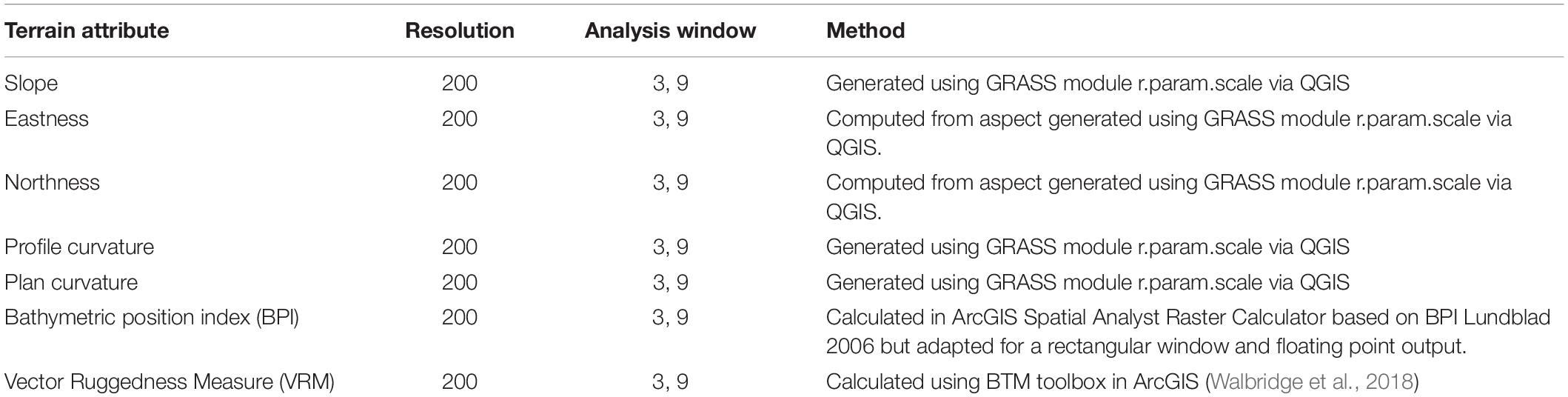
Table 1. Summary of terrain attributes generated from bathymetry data.

Oceanographic Model Data

The oceanographic model data used in this study come from a 1-year (2010) model simulation for the Barents Sea using 800 m × 800 m horizontal resolution (Figure 2). The model was set up using the bathymetry from IBCAO.v3 (International Bathymetric Chart of the Arctic Ocean, Jakobsson et al., 2012) and was run using the numerical ocean model ROMS (Regional Ocean Modeling System¹, e.g., Shchepetkin and McWilliams, 2005; Haidvogel et al., 2008) which applies a vertical topography-following coordinate system. Our simulation was defined with 35 vertical levels. Along the open boundaries, the model was forced with tidal analysis from TPXO7.2 (Egbert and Erofeeva, 2002) and daily averages of water level, salinity, temperature, and currents from the 4 km-model described in Lien et al. (2014). The atmospheric forcing applied was the ERA-Interim reanalysis provided by the European Centre for Medium-Range Weather Forecasts (ECMWF, see Dee et al., 2011). The model then provided information (maximum, mean, minimum, 90th percentile, standard deviation) on near-bottom temperature, salinity, and current speed. Data were resampled to 200 m using bilinear resampling to match the resolution of the terrain and geological data for onward use in biotope modeling.

FIGURE 2

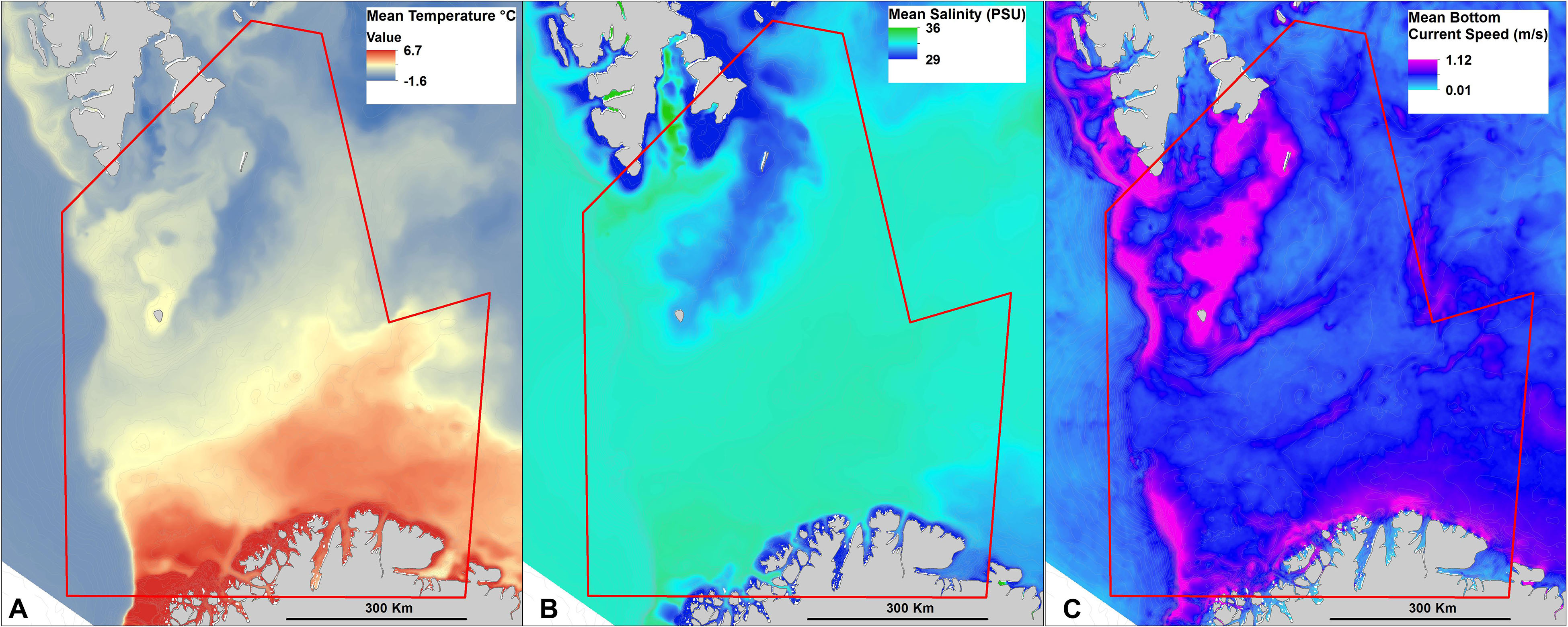
Figure 2. Examples of oceanographic variables indicating the level of detail captured by the Barents 800 model, and spatial variation in seabed oceanographical settings. (A) Mean temperature (°C), (B) mean salinity (PSU), and (C) mean bottom current speed (m/s).

Additional Variables

A number of variables derived from satellite observed ocean color were downloaded as raster datasets from MODIS-Aqua (Nasa Goddard Space Flight Center, 2018) using the Create Rasters for NASA OceanColor L3 SMI Product utility in the MGET toolbox (Roberts et al., 2010). While ocean color products represent surface conditions, they can have relevance for the seabed environment and have been used in several other seabed habitat mapping studies (e.g., Bryan and Metaxas, 2007; Davies et al., 2008; this issue). These data have a resolution of 4 km and represent annual average conditions. Data were downloaded for the entire time period over which MAREANO video surveys were conducted in this area, i.e., 2006–2017 and averaged over this time to create a single layer for each variable.

Latitude and longitude are not, strictly speaking, environmental variables but could be a proxy for biogeographic gradients or provinces, and may correlate with oceanographic variation, so these were also included in our analysis in the form of UTM33 (WGS84) easting and northing.

Classification Analyses

TWINSPAN

Video samples and species were classified using two-way indicator species analysis (TWINSPAN—Hill, 1979), as part of the software PCord 5.10. TWINSPAN is an algorithm which performs a divisive hierarchical ordination of site and species data. The data are ordered by the first axis of a correspondence analysis and then split near the middle, the location of the split being adjusted by the identification of indicator species with preferential affiliation to one half or the other (hereafter these halves are termed as “groups”). Each group is then iteratively split again using the same process, producing a hierarchical classification of site data with indicator species for each group. TWINSPAN, like detrended correspondence analysis (DCA), has been widely used by ecologists and has the potential to be particularly useful in HDM. The TWINSPAN method was selected also because it provides much clearer groupings of samples in a dataset with a large number of samples. The abundances of taxa in the video samples were square root transformed to down-weight the superabundant species and approximate a normal distribution. The transformed abundances were then placed into five abundance levels (called “pseudo-species” within the TWINSPAN terminology) using the following cut levels: >0–2, 2–5, 5–10, 10–20, and >20. All species that met the criteria described above were included in the analysis, but rare species were down weighted using the corresponding TWINSPAN function (meaning that they would be less likely to be chosen as an indicator species for each group). The TWINSPAN analysis then performs subsequent divisions of the dataset until the statistics are not able to distinguish any further divisions of groups. We applied an additional criterion that the resulting groups could not consist of too few samples. Groups with less than 20 samples were therefore merged with “parent groups” (lifted one division level). Terminal groups adhering to this rule were then considered to be our putative biotopes. As a result, some of the identified terminal groups, where merging with parent groups occurred, may more accurately represent “biotope complexes” which may include more than one distinguishable biotope if there were enough samples to properly define the community and correlated environmental parameters.

The TWINSPAN results also provided an overview of indicator species for each group based on species (and pseudo-species) composition. To refine the TWINSPAN-identified indicator species lists, expert knowledge was used to select those that are both dominant and easily identifiable from video footage. These species were considered to be representative of the new putative biotopes.

Environmental characteristics of TWINSPAN groups

An exploratory analysis was performed upon each TWINSPAN dichotomous split (i.e., pairings of groups) to investigate whether each group was correlated with any environmental variables. Draftsman plots, symbolizing each group in a pair and examining all variables from corresponding samples locations against depth together with key variable pairings such as temperature and salinity, enabled initial explorations of group/environment patterns. Principal component analyses (PCAs), comprising the most likely environmental correlates as identified by the draftsman plots and with points symbolized paired groups, were also used to indicate the dominant eigenvectors at each split (see Supplementary Information S1 for the main results of these investigations). In addition, forward selection analysis was performed using the software Canoco 5.04 to explore how much of the biological variation the different numerical environmental variables explained while using the biotopes as a categorical response variable. These analyses helped ensure that biologically relevant variables were pre-selected as potential predictor variables for subsequent modeling.

Modeling and Prediction of Spatial Biotope Distribution

To demonstrate the wider distribution of putative biotopes defined by TWINSPAN, a full coverage raster biotope map was produced using random forest models built using the Ranger package in R. This approach allows us to predict the distribution of biotopes between MAREANO stations providing full-coverage information in a format that is more convenient for onward use in management. Environmental predictor selection was decided based on the exploratory analyses described above, and a balance of model performance statistics and visual validation. The final model included the following 15 predictors: longitude, latitude, depth, average/s.d./max/min temperature, s.d. salinity, average/max/s.d. current speed, average chlorophyll, average POC, sediment, landscape. The model performance was evaluated using Cohen’s kappa coefficient which compares observed vs. expected accuracy (the proportion of correct predictions), while accounting for chance, and is a suitable performance statistic for multi-class problems. Further details of the modeling and prediction are beyond the scope of this paper and will be reported separately.

Results

Biotopes and Their Environmental Characteristics

The TWINSPAN analysis of the species data from all video samples split iteratively into groups is shown as a dendrogram in Figure 3. The TWINSPAN analysis generated a total of 27 groups adhering to our rule of >20 samples each (the smallest resulting group contained 23 samples). These groups became our putative biotopes (hereafter “biotopes”) and are described in Table 2 and represented by the letters A–Z and ZA in Figure 3.

FIGURE 3

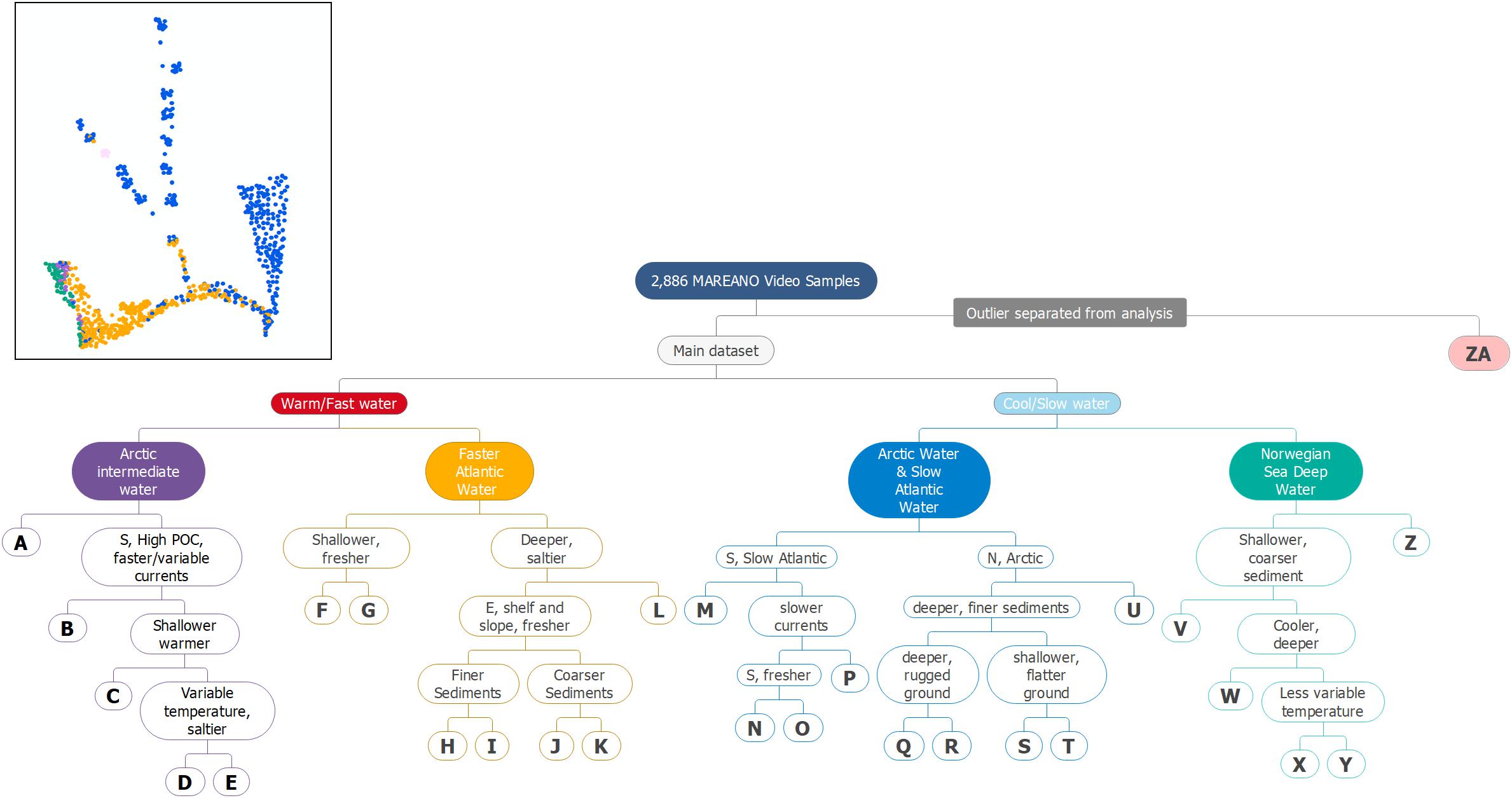
Figure 3. A cluster dendrogram visualizing the TWINSPAN analysis and possible dominant environmental drivers for splits after various ordinations. The letters A–ZA correspond to the putative biotopes described in Table 2. The inserted map shows the locations of samples of the five main groups identified at the third division level. The colors on the map correspond to the colors in the dendrogram.

TABLE 2

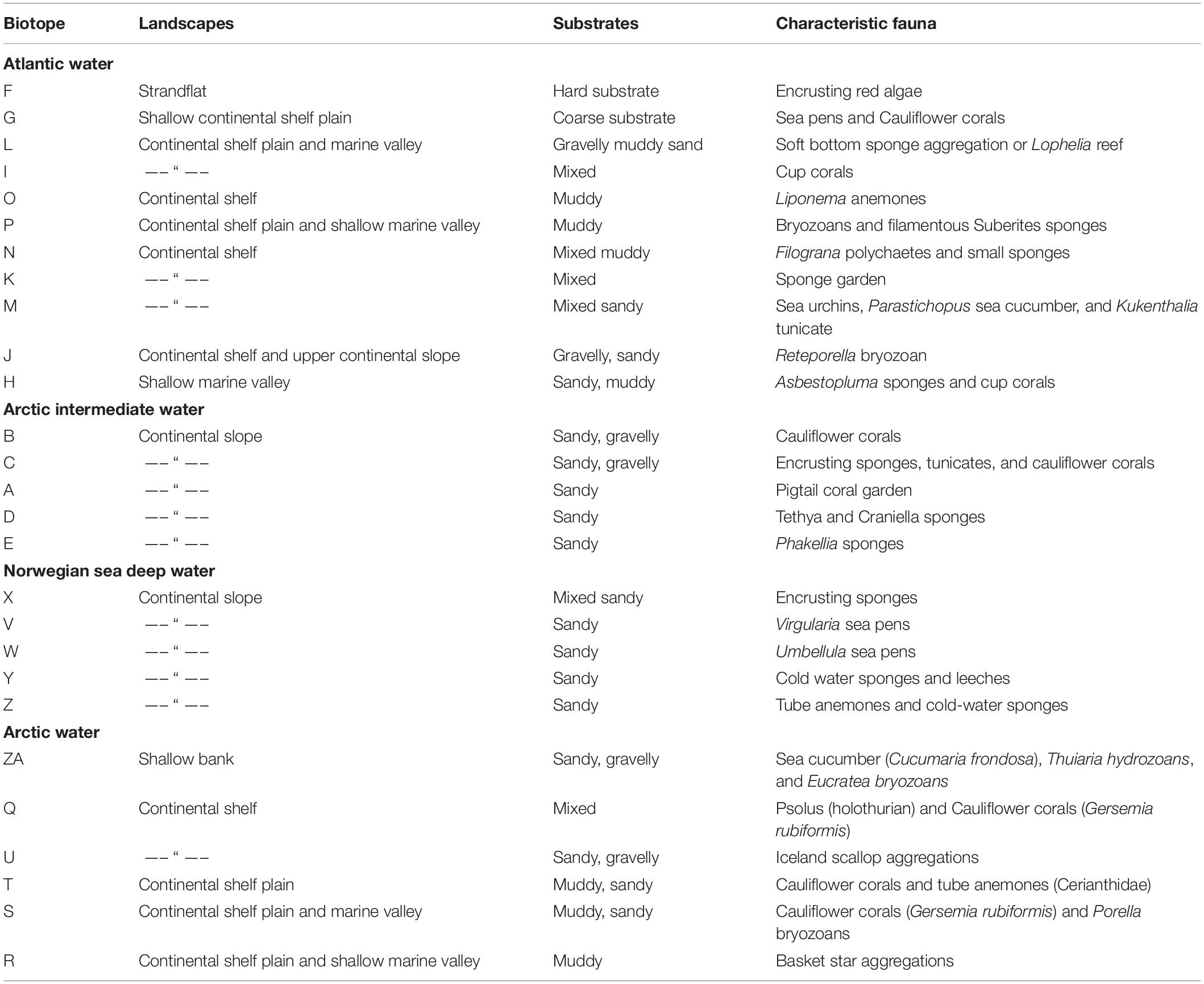
Table 2. List of biotopes, with a brief description of their characteristic water mass, landscapes, sediments, and fauna.

One group of locations at Spitsbergenbanken formed a clear outlier (biotope ZA, Figure 3). This biotope, characterized by the holothurian Cucumaria frondosa, bryozoan Eucratea loricata, and hydrozoan Thuiaria obsoleta on a shallow shell sand bank, was found to be distinct from all other groups due to its occurrence in an area of both high average current speeds and highly variable temperature and salinity (Figure 4).

FIGURE 4

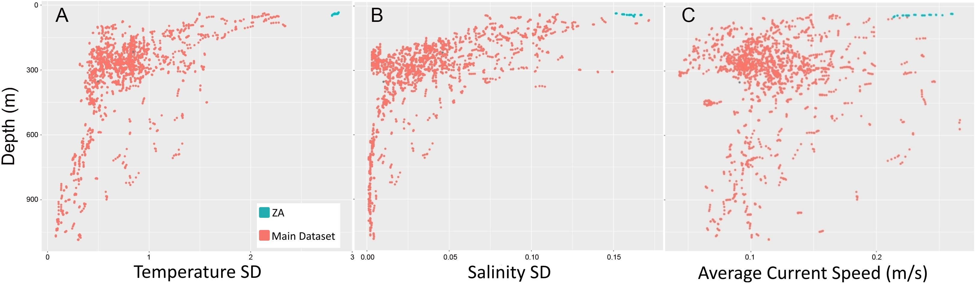
Figure 4. Plots showing the distinct conditions present at the Spitsbergenbanken sample sites (ZA) relative to the main dataset. (A) Temperature. (B) Salinity. (C) Average current speed. Subsequently, the ZA group was removed from the main analysis to better characterize communities found in more typical conditions.

The main analysis without the Spitsbergenbanken samples identified an additional 26 biotopes with different species compositions. Figure 3 also shows information on which of the environmental variables are correlated with each group at each split proceeding down the dendrogram.

The TWINSPAN analysis of the main dataset first divided into two main groups characterized by warm or fast flowing water (NAW and AIW) and cold or slow flowing water (AW and NSDW). An overview of the spatial distribution of these groups and biotope ZA is given in the inset map in Figure 3 to provide an indication of the spatial relevance of these clusters. Including the outlier, or singleton (Spitsbergenbanken, group ZA), the analysis indicated 12 biotopes in warm water/fast water masses (groups A-L in Figure 3 and Table 2), and 15 in cold/slow (M–Z and ZA). Similar cold-water species occurred both in the NSDW, below ca 700 m, and shallower in the Arctic water of the north eastern part of the study area. The next division level mainly separated deep (groups V–Z) and shallow (M–U) sites within these two cold and slow water groups while slope areas at intermediate depths (500–700 m) in the AIW (groups A–E) were separated from Atlantic shelf areas (F–L). Environmental correlates for biotopes identified by the first two divisions of the TWINSPAN hierarchy are illustrated in Figure 5. The colder and slower water masses represented five biotopes in NDSW (groups V–Z), five in Arctic Water (Q–U), and four in slower moving Atlantic water in the Southern Barents Sea (M–P). The warmer and faster water masses contained five biotopes in AIW (A–E), and seven in NAW (F–L). Further divisions reflected environments characterized by different variables including sediment and landscape types.

FIGURE 5

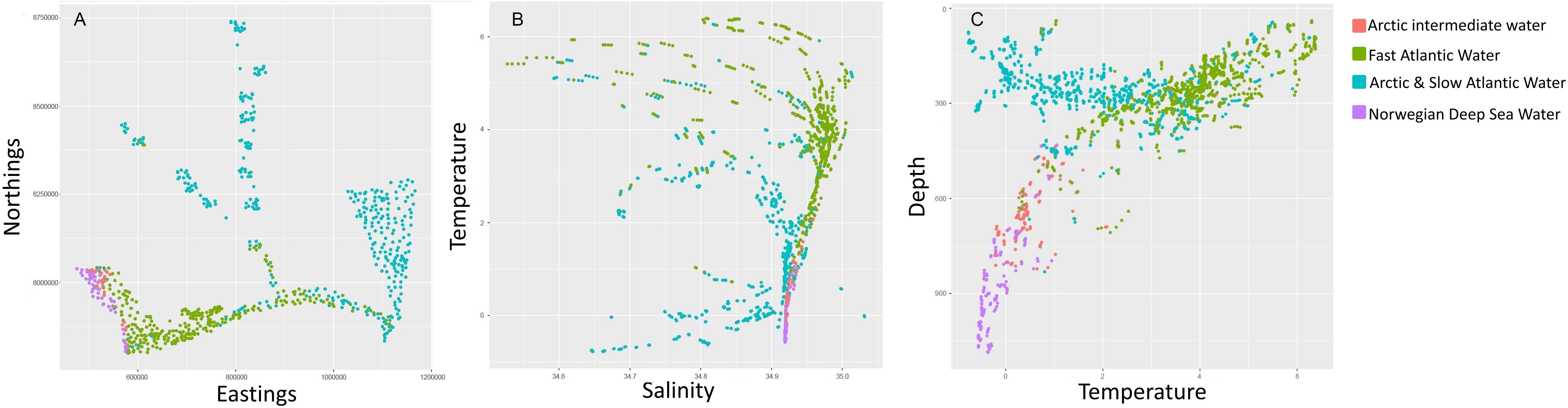
Figure 5. Example of environmental patterns of sample groups identified by the first two divisions of the TWINSPAN of the species dataset with the main clusters indicated in different colors. (A) Geographical distribution, (B) temperature vs. salinity, and (C) Depth vs. temperature.

A summary of the results of the forward selection analyses is presented in Table 3. The forward selection identified the variables with the highest explanatory power, without being strongly intercorrelated with each other, affecting the variance in TWINSPAN-defined biotope type. Latitude (UTM_Y), longitude (UTM_X) and bathymetry each contributed more than 10% toward the explanation of the variation between the TWINSPAN groups. Various oceanographic variables explained between 2 and 6% of the variation. Average chlorophyll was also among the 14 best variables suggesting a link with surface production. Of the terrain variables, only slope showed any explanatory potential. These results served as a starting point from which to guide the selection of predictors for biotope modeling, in conjunction with other methods.

TABLE 3

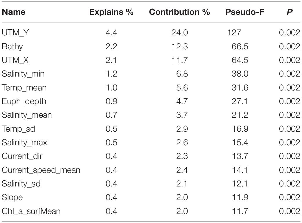
Table 3. Results from forward selection analysis of environmental data.

Taxonomic Composition of the Biotopes

A brief characterization of each biotope is given in Table 2, corresponding to letters in the dendrogram in Figure 3, with example images of selected contrasting biotopes given in Figure 6.

FIGURE 6

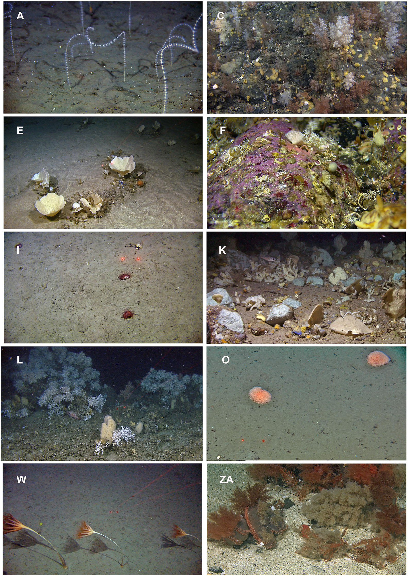
Figure 6. Examples of 10 contrasting biotopes identified by a TWINSPAN analysis of the species data from the video analyses. The letters represent the biotope abbreviation corresponding to Table 2. Arctic Intermediate Water Masses: (A) Soft bottom coral garden dominated by the pigtail coral (Radicipes gracilis) on the slope south west of Svalbard. (C) Encrusting sponges and tunicates and cauliflower corals on a gravelly bottom. (E) Sponge garden on sandy bottom dominated by Phakellia sp. and Axinella sp. Atlantic Water: (F) Hard substrates dominated by encrusting red algae in strandflat areas. (I) Mixed sediments dominated by cup corals (Flabellum macandrewi). (K) Sponge garden with a variety of axinellid sponges on mixed bottom. (L) Cold water coral reef (Lophelia pertusa) in the south western part of the study area. The same biotope complex is also represented by soft bottom sponge aggregations dominated by Geodidae sponges. (O) Muddy bottom on the shelf in central parts of the study area dominated by the anemone Liponema multicornis. Norwegian Sea Deep Water: (W) Sandy substrate on the lower slope dominated by the sea pen Umbellula encrinus. Arctic Water: (ZA) Shallow, sandy, gravelly bank dominated by the holothurian Cucumaria frondosa, the hydrozoan Thuiaria obsoleta, and the bryozoan Eucratea loricata.

Of the 11 biotopes in Atlantic Water (Figure 3, F–P) most of them (seven) occurred on mixed sediment types with occurrence of gravel in mixtures of sand and mud. Many of the characteristic taxa of these biotopes were sessile animals attached to hard substrate in the form of pebbles, cobbles, and shell fragments (e.g., anemones or sponges). In biotope P, although characterized by a predominance of mud, sessile bryozoans were characteristic. In most cases, these bryozoans (mainly Cyclostomatidae) seemed to be attached to fragments of bivalves or other calcareous organisms, but some seemed to occur as unattached colonies lying on the soft sediment. Of the biotopes characterized by hard and coarse bottoms (F and G), encrusting organisms (red algae in the shallow biotope F), and sessile organisms [cauliflower corals (Nephtheidae) in G] were dominant. Group L clearly represents a “biotope complex” and comprises observations of at least two likely biotopes including both soft bottom sponge gardens and Lophelia pertusa reefs. However, the latter in particular was represented by insufficient samples within the study area to permit a clear split into its own biotope during this analysis.

In the Arctic Intermediate Water on the continental slope (Figure 3, A–E) in the western part of the study area all biotopes represented sandy sediments where two (B and C) also contained gravel dominated, in part, by cauliflower corals. Of the biotopes on substrates dominated by sand: Biotope A was characterized by a pigtail coral (Radicipes gracilis). while the others were characterized by the sessile sponges Tethya and Craniella (D), and Phakellia sp. (E) attached to the few scattered pebbles or cobbles in the area.

The NSDW biotopes on the lower part of the continental slope in the western part of the study area (Figure 3, V–Z) contained mainly sandy sediments. Biotope X had sediment with content of gravel, providing substrate for characteristic encrusting sponges. Two types of sea pen dominated biotopes were found in this water mass (V and W). Biotope V was characterized by Virgularia sp. and W by Umbellula encrinus. The associated fauna within these sea pen biotopes were also different to each other. For instance, the burrowing amphipod Neohela monstrosa was common in the areas with Umbellula but was not observed in areas with Virgularia. Different Hexactinellid and carnivorous Poecilosclerid sponges characterized biotopes Y and Z.

The six biotopes identified in Arctic Water (Figure 3, Q–U and ZA) comprised varying substrates ranging from mud to mixed sediments with gravel (biotope Q). The basket star dominating biotope R was most likely Gorgonocephalus arcticus. Cauliflower corals were also characteristic of three of the arctic biotopes (S, T, and Q). The cauliflower corals of biotope S were unidentified but did not include Gersemia rubiformis which was present in biotopes S and Q. Biotope S and Q differed by dominance of the bryozoan Porella in biotope S and the sessile holothurian Psolus sp. in biotope Q. Biotope ZA was dominated by great abundances of the sea cucumber C. frondosa, the hydrozoan T. obsoleta, and the bryozoan E. loricata. Biotope U was characterized by the Iceland scallop (Chlamys islandica).

Spatial Distribution of Biotopes

All analyzed observation locations and their biotope assignments after TWINSPAN analysis are shown on the map in Figure 7. Here we see a detailed view of the biotope distribution following the major splits already indicated in Figure 3. Broadly biotope complex L appears to be dominant in the NAW, together with biotopes Y in the NSDW, A in the NSAIW, and Q in the Arctic Water. The arctic biotopes appear to largely sit north of the approximate location of the polar front, highlighting this biogeographic boundary. Figure 8 shows a map of the predicted distribution of biotopes in the Barents Sea based on models which combine the observed biotopes with the relevant environmental data. The final model had a Kappa value of 0.59 which is at the upper end of a moderate predictive performance across all biotopes—this seems reasonably good given the small percentage of raster pixels containing a biotope observation (<0.2%). We obtained higher (overestimated) performance statistics with standard methods (e.g., out of bag and cross-validation estimates), however, based on Meyer et al. (2018), we chose to use more conservative estimates which account for the ability of the model to predict to new locations.

FIGURE 7

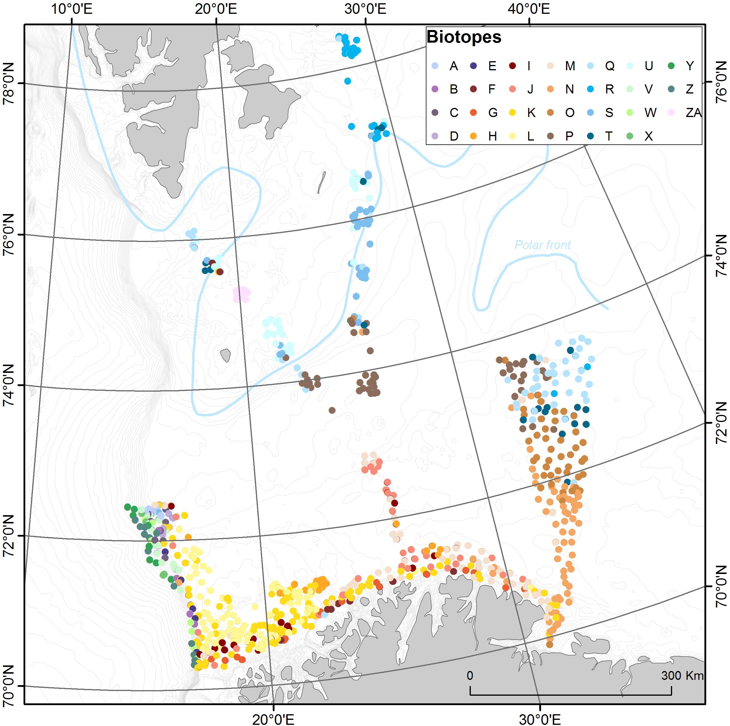
Figure 7. Distribution of video observation locations classified into 27 general biotopes. Colors are roughly grouped according to the water mass splits (greens = NDSW, purples = NSAIW, yellow/browns = NAW, blues = Arctic Water) (cf. Figure 3). An approximate location of the polar front is indicated with a blue line.

FIGURE 8

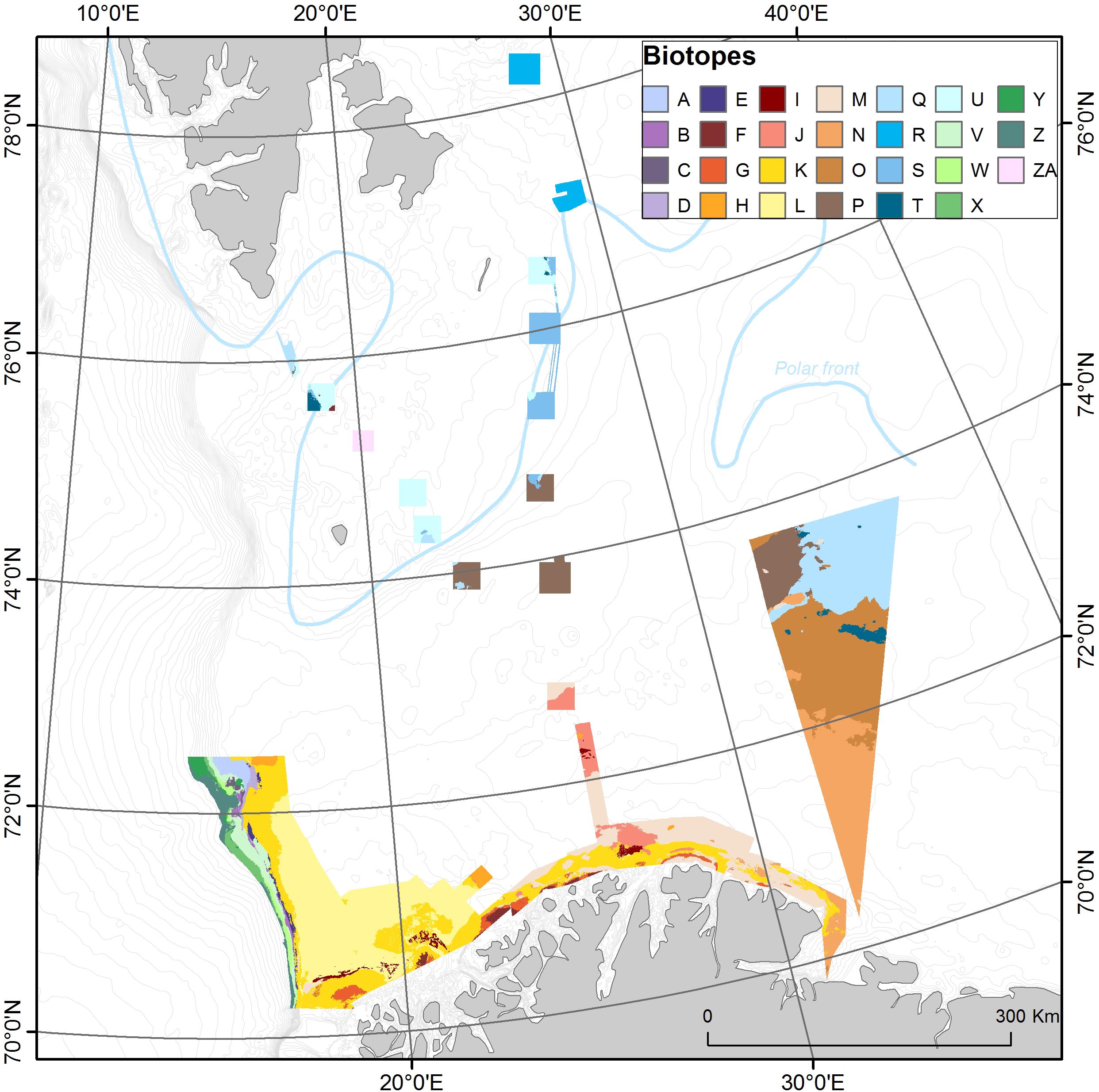
Figure 8. Predicted distribution of the 27 general biotopes. Colors are roughly grouped according to the water mass splits (greens = NDSW, purples = NSAIW, yellow/browns = NAW, blues = Arctic Water). The general location of the polar front is indicated with a blue line.

Discussion

The extensive sampling undertaken by the MAREANO project has allowed this first broadscale assessment of biotope characterization in the Barents Sea region. Our results reflect that this region spans a biogeographic boundary where warmer Atlantic water and related communities meets with Arctic waters and the polar front. This region is highly susceptible to climate change with indications of an “Atlantification” of the Barents Sea region (Barton, 2018; Lind et al., 2018) suggesting that this boundary is likely to move northward due to decreasing southward extension of the sea ice. The effect of this warming can have a severe effect on the arctic benthic communities, which as this study shows, are restricted to the colder and fresher Arctic water mass. The clear influence of water masses found in this study suggests either a dependence upon particular conditions (temperature, salinity, and/or nutrients) or a dispersal restriction imposed by water mass boundaries.

We note that certain biotopes are more restricted with respect to their environmental properties than others, i.e., they exist within a narrower range of conditions. These are generally easier to predict (have a lower rate of false predictions as assessed using the kappa coefficient), compared to those characterized by a wider range of environmental variation. However, the predictive ability is also influenced by the sample number and density within the biotope classes. Work is ongoing to provide a convenient and reliable method for communicating the degree of uncertainty associated with predicted the biotope distributions (map uncertainty), and also by attributing sample points with the certainty of their classification (classification uncertainty).

Due to the need for sufficient observations of each biotope for successful modeling, a few biotopes are less specific than might be desirable. Biotope complex L, which contains both sponge habitats and cold-water coral reefs, is an example of two distinct biotopes or habitats that have been recognized by numerous studies in the past (e.g., Davies et al., 2008; Ramirez Llodra et al., 2011). These usually distinct biotopes group together in our analyses probably because they (1) share a great number of taxa such as redfish (Sebastes spp.), several sponges (e.g., Geodidae and Axinellidae), sea urchins, and sea stars, and (2) that the number of video samples within one of these communities (the coral reefs) is too low. We expect that these classes would separate should they be analyzed together with locations from within the core distribution areas of cold-water corals. Similarly, biotope ZA present on Spitsbergenbanken appears to be unique to this mapped area, and fortunately had sufficient samples to be retained as a distinct biotope class. However, we note that no similar environments have yet been mapped by MAREANO so its extent is as yet unknown. It is possible that there could be other locations with similar conditions where this community could be encountered, most likely on other shallow banks where the Barents Sea and Norwegian Sea meet. Future explorations of the area and/or extended predictions when further data become available may be able to clarify how unique this community is. These examples illustrate how it is important to consider the limitations of sampling and mapping areas covered when assessing the results of biotope mapping.

Due to the large area mapped and volume of samples used, the methods for defining biotopes and subsequently modeling their distribution have been updated from those used in previous MAREANO biotope maps. The new TWINSPAN approach is well matched to processing larger datasets and will form the basis of updating MAREANO general biotope maps in other areas (all MAREANO map products are available via www.mareano.no). We note that TWINSPAN and other methods may not fully agree in the number of groups defined, and other methods may be better suited when analyzing smaller datasets (Anderson and Clements, 2000), yet the clear environmental correlates with the TWINSPAN splits in this study suggest that this tool is adequate for the purposes of mapping communities in this region.

The environmental variables used to assess the TWINSPAN splits were evaluated at the resolution that would subsequently be used for the modeling. Those variables generated from broader-scale neighborhood analyses may miss some finer scale effects, but also offer some valuable assessment of larger geomorphological influences that would otherwise be overlooked. Although the resampling of the original bathymetric data to 200 m means that finer-scale terrain variability is lost this resolution still allows us to capture the variations that match the length of video samples (200 m). Early MAREANO biotope maps were produced before oceanographic model data were available, while recent maps including the current study use oceanographic models originating from 800 m resolution. Resampling of model data from 800 to 200 m introduces minimal pseudo-variation from interpolating to a finer scale. Note that the values come from the lowest layer in a surface-optimized multi-layer ROMS model. The values therefore represent conditions spanning meters to tens of meters above the seabed depending on depth, rather than a fixed depth from the seabed. A 200 m scale is also well suited to raster-representation of the geological maps, which are produced at 1:100,000 scale and coarser, and therefore do not contain information on fine-scale variations at sub-200 m scales. In addition, we note that reduction of the bathymetry data to 200 m resolution overcomes certain acquisition-related artifacts associated with the bathymetry data in deeper waters, which are problematic for terrain analysis at finer scales and could produce misleading results when predicting habitat distribution (Lecours et al., 2017).

While the biotope classification (Figure 3) and observed spatial distribution (Figure 7) represent the main results of this study, the predicted biotope map is presented here (Figure 8) to provide a further indication of the varied environment and benthic communities present across the Barents Sea, including many areas previously undocumented at this scale. The results demonstrate that there is a clear biogeographic boundary for benthic communities related to the Polar front. Several cold-water biotopes toward the north and east in the study area are quite distinct from those in Atlantic water or NSDW. Temperature is probably the most important of the factors causing the biotic differences, as it is also a contributor to the strong effects of Latitude (UTM_Y) and Depth (Bathy) in the forward selection (see Table 2). However, different larval transport routes associated with the water masses may control the larval supply from different biogeographic and climatic regions. Overall, we note that the influence of major water masses is clearly important in controlling biotope distribution with oceanographic variables being among the most important. Other studies have also found oceanographic variables to be highly influential in models of species distribution (e.g., Yesson et al., 2012). This is likely because terrain variables, while easier to obtain as full coverage datasets, are often acting as a proxy for oceanographic variables such as temperature and current speed, and in some areas inadequately so. The oceanographic variables naturally relate to species tolerance and physiological functioning (e.g., temperature and salinity), as well as conditions that may affect food availability and access (e.g., current speeds).

The continued importance of geographic variables (location) suggests that they act as proxies to more directly influencing factors on benthic communities, and that there are other variables besides those used in the present model that may be more relevant to biotope distribution. In the meantime, the geographic variables appear to provide adequate proxies to capture some of these influences until such time as the relevant data are identified and made available for use in future models. The spatial scale of the response variables (biotope class) should ideally reflect the patchiness of the characteristic species. The scale used for megafauna composition in this study (200 m video sequences) will in many cases capture areas comprising different patches of sub-communities whose distribution reflects local fine scale variation in bottom substrate composition and local topography within the biotope. The biotopes described and modeled in this study may therefore be regarded as “local ecounits” where some represent areas with occurrence of several distinct sub-communities mosaiced due to patchiness. Although some biotopes do commonly occur as patches far larger than the sampling size. For instance, on level soft bottoms with a homogenous substrate composition fields of sea pens, scattered smaller sponges, anemones, or polychaetes may extend continuously over several hundreds of meters.

Conclusion

Twenty-seven biotopes were identified by applying TWINSPAN to quantitative species data obtained from analyses of seabed video records. The groups represented different environments with the main clusters related to water mass, landscape, and sediment composition. This enhanced the detection of different biogeographic regions, here likely related to the Polar Front, and provided a basis for better predictive modeling of seabed communities spanning a biogeographic boundary. The classification of benthic habitats in the deep sea has been limited by broad scale information about environmental factors acting at a local scale. The environmental variation is not uniform, and the variation in community composition will reflect this. Thus, biotope mapping of larger areas faces a challenge of representing a multitude of spatial scales. In this study, we have demonstrated that the dominating substrate is not always reflected in the community composition, as sessile organisms may appear as characteristic taxa even with a very low contribution of hard substrate. The oceanographic setting and probably also biological factors such as food availability and larval transport is of great importance for the control of species composition of epibenthic megafauna. Better knowledge of these factors could improve the models of biotope distribution further.

Data Availability Statement

The original contributions presented in the study are included in the article/Supplementary Material, further inquiries can be directed to the corresponding author.

Author Contributions

PB-M contributed to video analyses, statistical analyses, figures, and writing. MD contributed to modeling, figures, and writing. RR contributed to statistical analyses, figures, and writing. GG-M contributed to statistical analyses and writing. LB-M and LB contributed to writing. JA contributed to oceanographical modeling and writing.

Funding

This research was carried out as part of the Norwegian national seabed mapping program MAREANO, funded directly from the Norwegian Government.

Conflict of Interest

The authors declare that the research was conducted in the absence of any commercial or financial relationships that could be construed as a potential conflict of interest.

Acknowledgments

We acknowledge the video analysts at IMR for their patient annotations of more than 500 h of seabed video. Thanks to all participants of the MAREANO program (www.mareano.no) for their input to this article. The multibeam data were acquired and supplied by the Norwegian Hydrographic Service (Kartverket). The data are released under a Creative Commons Attribution 4.0 International (CC BY 4.0): https://creativecommons.org/licenses/by/4.0/. The ocean model simulation was performed on resources provided by UNINETT Sigma2—the National Infrastructure for High Performance Computing and Data Storage in Norway. We also thank the two reviewers and our editor, Daphne Cuvelier, for their time and assistance in making this manuscript stronger.

Supplementary Material

The Supplementary Material for this article can be found online at: https://www.frontiersin.org/articles/10.3389/fmars.2020.00271/full#supplementary-material

INFORMATION S1 | Draftsman plots and PCAs demonstrating the potential environmental drivers behind each TWINSPAN split.

Footnotes

1. ^ http://myroms.org

References

Anderson, M. J., and Clements, A. M. (2000). Resolving environmental disputes: a statistical method for choosing among competing cluster models. Ecol. Appl. 10, 1341–1355. doi: 10.1890/1051-0761(2000)010[1341:redasm]2.0.co;2

CrossRef Full Text | Google Scholar

Barnes, R. S. K., and Hughes, R. N. (1982). An Introduction to Marine Ecology. Oxford: Blackwell Scientific.

Google Scholar

Barton, B. I. (2018). Observed atlantification of the Barents Sea causes the polar front to limit the expansion of Winter Sea Ice. J. Phys. Oceanogr. 48, 1849–1866. doi: 10.1175/JPO-D-18-0003.1

CrossRef Full Text | Google Scholar

Bellec, V. K., Bøe, R., Bjarnadóttir, L. R., Albretsen, J., Dolan, M., Chand, S., et al. (2019). Sandbanks, sandwaves and megaripples on Spitsbergenbanken, Barents Sea. Mar. Geol. 416:105998. doi: 10.1016/j.margeo.2019.105998

CrossRef Full Text | Google Scholar

Bjarnadóttir, L. R., Winsborrow, M. C. M., and Andreassen, K. (2014). Deglaciation of the central Barents Sea. Quat. Sci. Rev. 92, 2018–2226.

Google Scholar

Blindheim, J. (1990). Arctic intermediate water in the Norwegian Sea. Deep Sea Res. 37, 1475–1489. doi: 10.1016/0198-0149(90)90138-L

CrossRef Full Text | Google Scholar

Bryan, T. L., and Metaxas, A. (2007). Predicting suitable habitat for deep-water gorgonian corals on the Atlantic and Pacific Continental Margins of North America. Mar. Ecol. Prog. Ser. 330, 113–126. doi: 10.3354/meps330113

CrossRef Full Text | Google Scholar

Buhl-Mortensen, L., and Buhl-Mortensen, P. (2017). Marine litter in the Nordic Seas: distribution composition and abundance. Mar. Pollut. Bull. 125, 260–270. doi: 10.1016/j.marpolbul.2017.08.048

CrossRef Full Text | Google Scholar

Buhl-Mortensen, L., Buhl-Mortensen, P., Dolan, M. F. J., and Holte, B. (2015a). The MAREANO programme – A full coverage mapping of the Norwegian off-shore benthic environment and fauna. Mar. Biol. Res. 11, 4–17. doi: 10.1080/17451000.2014.952312

CrossRef Full Text | Google Scholar

Buhl-Mortensen, L., Buhl-Mortensen, P., Dolan, M. F. J., and Gonzalez-Mirelis, G. (2015b). Habitat mapping as a tool for conservation and sustainable use of marine resources: some perspectives from the MAREANO Programme, Norway. J. Sea Res. 100, 46–61. doi: 10.1016/j.marpolbul.2017.08.04810.1016/j.seares.2014.10.014

CrossRef Full Text | Google Scholar

Buhl-Mortensen, L., Olsen, E., Røttingen, I., Buhl-Mortensen, P., Hoel, A. H., Lid, S. R., et al. (2012). Application of the MESMA Framework. Case Study: The Barents Sea. MESMA report, 138.

Google Scholar

Buhl-Mortensen, P., Buhl-Mortensen, L., Dolan, M., Dannheim, J., and Kröger, K. (2009). Megafaunal diversity associated with marine landscapes of northern Norway: a preliminary assessment. Norw. J. Geol. 89, 163–171.

Google Scholar

Davies, A. J., Wisshak, M., Orr, J. C., and Roberts, J. M. (2008). Predicting suitable habitat for the cold-water coral Lophelia pertusa (Scleractinia). Deep Sea Res. I 55, 1048–1062. doi: 10.1016/j.dsr.2008.04.010

CrossRef Full Text | Google Scholar

Dee, D. P., Uppala, S. M., Simmons, A. J., Berrisford, P., Poli, P., Kobayashi, S., et al. (2011). The ERA-Interim reanalysis: configuration and performance of the data assimilation system. Q. J. R. Meteorol. Soc. 137, 553–597. doi: 10.1002/qj.828

CrossRef Full Text | Google Scholar

Dolan, M. F. J., and Lucieer, V. L. (2014). Variation and uncertainty in bathymetric slope calculations using geographic information systems. J. Mar. Geodesy 37, 187–219. doi: 10.1080/01490419.2014.902888

CrossRef Full Text | Google Scholar

Egbert, G. D., and Erofeeva, S. Y. (2002). Efficient inverse modeling of barotropic ocean tides. J. Atmos. Ocean. Technol. 19, 183–204. doi: 10.1175/1520-0426(2002)019<0183:eimobo>2.0.co;2

CrossRef Full Text | Google Scholar

Elvenes, S. (2013). Landscape Mapping in MAREANO. NGU Report 2013.035.. Available online at: https://www.ngu.no/upload/Publikasjoner/Rapporter/2013/2013_035.pdf (accessed April 14, 2020).

Google Scholar

Elverhøi, A., Fjeldskaar, W., Solheim, A., Nyland-Berg, M., and Russwurm, L. (1993). maximum. Quat. Sci. Rev. 12, 863–873.

Google Scholar

Geological Survey of Norway [NGU] (2019a). Marine – Seabed Sediments (Grain Size), Regional. Available online at: http://geo.ngu.no/download/order?lang=en&dataset=701 (accessed January 7, 2019).

Google Scholar

Geological Survey of Norway [NGU] (2019b). Marine Landscapes. Available online at: http://geo.ngu.no/download/order?lang=en&dataset=705 (accessed January 7, 2019).

Google Scholar

Gomes Pereira, J. N., Auger, V., Beisiegel, K., Benjamin, R., Bergmann, M., Bowden, D., et al. (2016). Current and future trends in marine image annotation software. Prog. Oceanogr. 149, 106–120.

Google Scholar

Haidvogel, D. B., Arango, W. P., Budgell, B. D., Cornuelle, E., Curchitser, E., Di Lorenzo, K., et al. (2008). Ocean forecasting in terrain-following coordinates: formulation and skill assessment of the regional ocean modeling system. J. Comp. Phys. 227, 3595–3624. doi: 10.1016/j.jcp.2007.06.016

CrossRef Full Text | Google Scholar

Hansen, B., and Østerhus, S. (2000). North Atlantic-Nordic Seas exchanges. Prog. Oceanogr. 45, 109–208. doi: 10.1016/s0079-6611(99)00052-x

CrossRef Full Text | Google Scholar

Harris, P. T. (2012). “Biogeography, benthic ecology, and habitat classification schemes,” in Seafloor Geomorphology as Benthic Habitat: Geohab Atlas of Seafloor Geomorphic Features and Benthic Habitats, 1st Edn, eds P. T. Harris and E. Baker (Boston: Elsevier), 61–91. doi: 10.1016/b978-0-12-385140-6.00004-9

CrossRef Full Text | Google Scholar

Harris, P. T., and Baker, E. K. (2011). Seafloor Geomorphology as Benthic Habitat: GeoHab Atlas of Seafloor Geomorphic Features and Benthic Habitats. Amsterdam: Elsevier.

Google Scholar

Hill, M. O. (1979). TWINSPAN a Fortran Program for Arranging Multivariate Data in an Ordered Two-Way Table by Classification of the Individuals and Attributes. Ecology and Systematic. Ithaca, NY: Cornell University.

Google Scholar

Ingvaldsen, R., and Loeng, H. (2009). “Physical oceanography,” in Ecosystem Barents Sea. Vol. 2009 Tapir, eds E. Sakshaug, G. Johnsen, and K. Kovacs (Trondheim: Academic Press).

Google Scholar

Jakobsson, M., Mayer, L. A., Coakley, B., Dowdeswell, J. A., Forbes, S., Fridman, B., et al. (2012). The international bathymetric chart of the arctic ocean (IBCAO) version 3.0. Geophys. Res. Lett. 39:L12609. doi: 10.1029/2012GL052219

CrossRef Full Text | Google Scholar

Knies, J., Matthiesen, J., Vogt, C., Laberg, J. S., Hjelstuen, B. O., Smelror, M., et al. (2009). The Plio-Pleistocene glaciation of the Barents Sea-Svalbard region: a new model based on revised chronostratigraphy. Quat. Sci. Rev. 10, 1–18.

Google Scholar

Lecours, V., Brown, C. J., Devillers, R., Lucieer, V. L., and Edinger, E. N. (2016). Comparing selections of environmental variables for ecological studies: a focus on terrain attributes. PLoS One 12:e0167128. doi: 10.1371/journal.pone.0167128

CrossRef Full Text | Google Scholar

Lecours, V., Devillers, R., Edinger, E. N., Brown, C. J., and Lucieer, V. L. (2017). Influence of artefacts in marine digital terrain models on habitat maps and species distribution models: a multiscale assessment. Remote Sens. Ecol. Conserv. 3, 232–246. doi: 10.1002/rse2.49

CrossRef Full Text | Google Scholar

Lien, V. S., Gusdal, Y., and Vikebø, F. B. (2014). Along-shelf hydrographic anomalies in the Nordic Seas (1960–2011): locally generated or advective signals? Ocean Dyn. 64, 1047–1059. doi: 10.1007/s10236-014-0736-3

CrossRef Full Text | Google Scholar

Lind, S., Ingvaldsen, R. B., and Furevik, T. (2018). Arctic warming hotspot in the northern Barents Sea linked to declining sea-ice import. Nat. Clim. Change 8, 634–639. doi: 10.1038/s41558-018-0205-y

CrossRef Full Text | Google Scholar

Loeng, H. (1991). Features of the physical oceanographic conditions of the Barents Sea. Polar Res. 10, 5–18. doi: 10.1111/j.1751-8369.1991.tb00630.x

CrossRef Full Text | Google Scholar

McCauley, D. J. (2015). Marine defaunation: animal loss in the global ocean. Proc. Natl. Acad. Sci. U.S.A. 347:1255641. doi: 10.1126/science.1255641

CrossRef Full Text | Google Scholar

Meyer, H., Reudenbach, C., Hengl, T., Katurji, M., and Nauss, T. (2018). Improving performance of spatio-temporal machine learning models using forward feature selection and target-oriented validation. Environ. Model. Softw. 101, 1–9. doi: 10.1016/j.envsoft.2017.12.001

CrossRef Full Text | Google Scholar

Mortensen, P. B., and Buhl-Mortensen, L. (2005). “Coral habitats in The Gully, a submarine canyon off Atlantic Canada,” in Cold-water Corals and Ecosystems, eds A. Freiwald and J. M. Roberts (Berlin: Springer-Verlag), 247–277. doi: 10.1007/3-540-27673-4_12

CrossRef Full Text | Google Scholar

Nasa Goddard Space Flight Center (2018). NASA Goddard Space Flight Center, Ocean Ecology Laboratory, Ocean Biology Processing Group. Greenbelt, MD: MODIS.

Google Scholar

Ozhigin, V. K., Ingvaldsen, R. B., Loeng, H., Boitsov, V., and Karsakov, A. (2011). “Introduction to the Barents Sea,” in The Barents Sea. Ecosystem, Resources, Management. Half a Century of Russian-Norwegian Cooperation, eds T. Jakobsen and V. K. Ozhigin (Trondheim: Tapir Academic Press), 315–328.

Google Scholar

Ramirez Llodra, E., Tyler, P. A., Baker, M. C., Bergstad, O. A., Clark, M. R., Escobar, E., et al. (2011). Man and the last great wilderness: human impact on the Deep Sea. PLoS One 6:e22588. doi: 10.1371/journal.pone.0022588

CrossRef Full Text | Google Scholar

Roberts, J. J., Best, B. D., Dunn, D. C., Treml, E. A., and Halpin, P. N. (2010). Marine geospatial ecology tools: an integrated framework for ecological geoprocessing with ArcGIS, Python, R, MATLAB, and C++. Environ. Model. Softw. 25, 1197–1207. doi: 10.1016/j.envsoft.2010.03.029

CrossRef Full Text | Google Scholar

Ross, R. E., and Howell, K. L. (2013). Use of predictive habitat modelling to assess the distribution and extent of the current protection of ‘listed’ deep-sea habitats. Divers. Distrib. 19, 433–445. doi: 10.1111/ddi.12010

CrossRef Full Text | Google Scholar

Shchepetkin, A. F., and McWilliams, J. C. (2005). The regional ocean modeling system (ROMS): a split-explicit, free-surface, topography-following coordinates ocean model. Ocean Model. 9, 347–404. doi: 10.1016/j.ocemod.2004.08.002

CrossRef Full Text | Google Scholar

Sigmond, E. M. O. (2002). Geological Map, Land and Sea Areas of Northern Europe, Scale 1:4 Million. Trondheim: Geological Survey of Norway.

Google Scholar

Skagseth, Ø (2008). Recirculation of Atlantic Water in the western Barents Sea. Geophys. Res. Lett. 35:L11606. doi: 10.1029/2008GL033785

CrossRef Full Text | Google Scholar

Steltzenmüller, W., Breen, P., Stamford, T., Thomsen, F., Badalamenti, F., Borja, A., et al. (2013). Monitoring and evaluating of spatially managed areas: a generic framework for implementation of ecosystem based marine management and its application. Mar. Pollut. Bull. 37, 149–164. doi: 10.1016/j.marpol.2012.04.012

CrossRef Full Text | Google Scholar

Walbridge, S., Slocum, N., Pobuda, M., and Wright, D. (2018). Unified geomorphological analysis workflows with benthic terrain modeler. Geosciences 8:94. doi: 10.3390/geosciences8030094

CrossRef Full Text | Google Scholar

Wilson, M. F. J., O’Connell, B., Brown, C., Guinan, J. C., and Grehan, A. J. (2007). Multiscale terrain analysis of multibeam bathymetry data for habitat mapping on the continental slope. Mar. Geodesy 30, 3–35. doi: 10.1080/01490410701295962

CrossRef Full Text | Google Scholar

Yesson, C., Taylor, M. L., Tittensor, D. P., Davies, A. J., Guinotte, J., Baco, A., et al. (2012). Global habitat suitability of cold-water octocorals. J. Biogeogr. 39, 1278–1292. doi: 10.1111/j.1365-2699.2011.02681.x

CrossRef Full Text | Google Scholar