Habitat Partitioning in Sympatric Delphinids Around the Falkland Islands: Predicting Distributions Based on a Limited Data Set

Introduction

Understanding how environmental factors shape species distributions is a key concept in ecology. Characterising species-environment relationships can facilitate accurate predictions of species’ spatial distributions (Guisan and Zimmermann, 2000), and help identify ecological niches (Austin et al., 1990; Barragán-Barrera et al., 2019). Knowing where animals occur within a specific region is also crucial for effective management and for the implementation of conservation measures (Guisan et al., 2013). Ideally, the entire area of interest is surveyed in order to estimate the distribution of animals. However, survey data may be very costly to obtain and are restricted to times and areas where direct observations are possible. To overcome this spatial limitation, such data can be analysed together with associated habitat covariates, and the resulting models used to predict where animals could be, as long as the surveyed area has covered similar environmental conditions to that of the region of interest (Guisan and Zimmermann, 2000; Mannocci et al., 2014).

One such area where surveys in the complex marine environment are challenging, is around the Falkland (also known as Malvinas) Islands (FI) in the South Atlantic. The FI are situated on the Patagonian Shelf and include the two main islands, East Falkland and West Falkland, and 776 smaller islands. The coast is convoluted and lined by extensive kelp beds (Macrocystis and Lessonia spp.), which can extend up to 10 km offshore, and cover an area of around 1,600 km². These inshore waters are important to a community of marine animals including meso predators such as Commerson’s dolphins (Cephalorhynchus commersonii) and Peale’s dolphins (Lagenorhynchus australis). The current lack of information on the distribution and habitat use of Commerson’s and Peale’s dolphins in FI waters limits the proper assessment of their conservation status at national, regional and international levels as well as their inclusion in local and regional management plans (Augé et al., 2018). Both are key species in the FI Species Action Plans (Otley, 2008), requiring population assessments and baseline understanding of their ecology so that they can be included in wider marine spatial planning initiatives. The shelf area around the FI has experienced a substantial increase in anthropogenic activities including oil exploration, shipping traffic, commercial fishing, aquaculture, and tourism (Otley, 2008; Augé et al., 2018). Such activities often negatively affect marine ecosystem stability and functioning, and thus should be carefully assessed and managed, requiring information on spatial overlap between species distributions and anthropogenic activities. Commercial fishing and aquaculture are still in their infancy in the FI inshore waters, providing a relatively rare opportunity to investigate species distributions prior to the onset of these potentially damaging human activities.

Commerson’s and Peale’s dolphins inhabit continental shelf waters ranging from shallow nearshore to offshore waters up to 300 m deep (Dellabianca et al., 2016; Cipriano, 2018), and are often considered to be sympatric species in the South Atlantic, including the FI. Peale’s dolphins make extensive use of kelp beds for foraging (Viddi and Lescrauwaet, 2005), and their diet is known to consist of bottom and demersal fishes as well as octopus and squid species living on the continental shelf or associated with kelp (Schiavini et al., 1997). A similar diet composition was also found for Commerson’s dolphins inhabiting the same region (Riccialdelli et al., 2010). Commerson’s dolphins have been observed in estuarine zones feeding in shallow waters near river mouths where their distribution is influenced by tidal patterns (Garaffo et al., 2011; de Castro et al., 2013). Tidal fronts are a dominant oceanographic feature around the FI (Acha et al., 2004). Frontal areas are associated with high primary productivity, and usually attract diverse low and high trophic level consumers, including meso or top predators such as dolphins (Davis et al., 2002; Dellabianca et al., 2012). Modelled distribution for both Commerson’s and Peale’s dolphins matched previously described frontal zones on the Patagonian shelf (Acha et al., 2004; Dellabianca et al., 2016), but such relationships have not yet been investigated in other parts of the species’ ranges.

The aim of this study was to make use of a spatially limited dataset to investigate habitat use of Commerson’s and Peale’s dolphins in the entire FI inshore waters. Firstly, we describe the relationships between habitat covariates and sightings of dolphins based on data from a systematic small-scale survey. Secondly, we predict the spatial distributions of both species throughout the FI inshore waters, using a Hurdle model approach. We use the model predictions to identify key areas for both species, and examine spatial overlap between preferred habitats. We demonstrate the usefulness of our methodology for predictive habitat modelling, which should be relevant to other complex areas and data-poor species.

Materials and Methods

Sighting Data

Sightings of Commerson’s and Peale’s dolphins were collected during a 10-day vessel-based line transect survey conducted from the 26th of February to the 7th of March 2014 and implemented as part of the Darwin Initiative UK Overseas Territories Challenge Fund Project “Inshore Cetaceans of the Falkland Islands” (Project Reference: EIDCF019; Thomsen, 2013). Surveys were conducted with a 15 m converted fishing vessel (MV Condor) which housed the observation team. During surveys, two dedicated observers scanned continuously ahead of the vessel and out to 90° of the track line using the naked eye aided by 7 × 50 binoculars when needed. For each sighting, species identification, estimated group size, behaviour, distance and angle to the sighting (using measuring sticks and angle boards, respectively) as well as sighting conditions were reported to a third observer inside the wheelhouse who recorded these data in the bespoke software Logger (Gillespie et al., 2010) along with the date, time and the vessel’s GPS location.

Due to time and budget constraints the survey could only cover a small but representative part of the FI inshore waters (Thomsen, 2013). The survey area comprised the different coastal habitat types around the FI, and encompassed approximately 2,000 km² split into nine smaller regions or strata containing 72 transect lines (extending from 0.3 to 10 km offshore), located in the northern part of West Falkland, the northern part of Falkland Sound, and the southern part of East Falkland (Figure 1). The survey was designed using the software Distance v.6 (Thomas et al., 2010). Average vessel steaming speed was 8 knots (Thomsen, 2014).

FIGURE 1

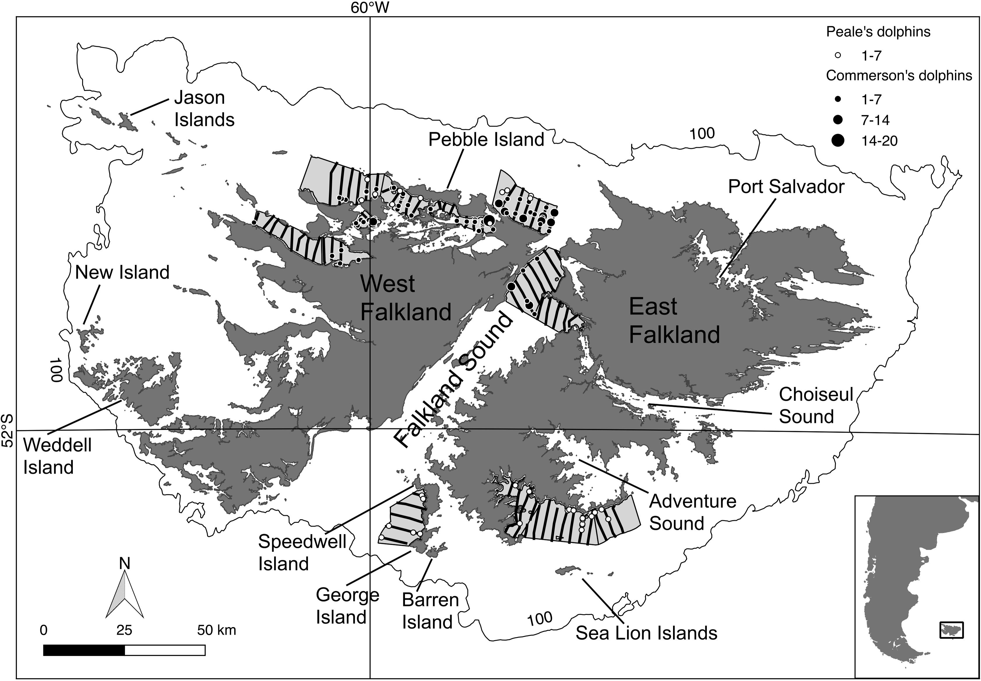
Figure 1. Transect lines travelled during the 2014 ship-based survey (in black). Round symbols = sightings for Commerson’s (black) and Peale’s (white) dolphins. Symbol size is proportional to the observed group size. Light-grey polygons = surveyed area, outer line = 100 m isobath. Inset map: Falkland Islands in relation to South America.

Aerial line-transect surveys with a fixed wing aircraft were conducted during nine days from March to May 2017 using two trained observers and one data recorder. Software Distance v.6.2. was used to design the survey to cover the entire FI inshore waters resulting in 217 parallel transect lines (extending from the coast to 10 km offshore; Supplementary Figure 1). The aircraft flew at a height of 150 m at a speed of 90 knots (∼167 km/h).

All field work was carried out in accordance with the guidelines for the Treatment of Marine Mammals in Field Research (Society for Marine Mammalogy) and approved by the University of St Andrews, School of Biology Animal Ethics Committee.

Habitat Covariates

To model dolphin habitat preference, we considered six environmental covariates: distance to coast (DC), distance to kelp (DK), distance to 100 m isobath (D100), distance to main river mouths (DRM), water depth, and water column stratification index (SI). These abiotic variables were considered proxies characterising biologically relevant yet unknown links between dolphins and their environment (e.g., via prey distribution) and had been shown or were suspected to be of importance to either species (Garaffo et al., 2011; de Castro et al., 2013; Dellabianca et al., 2016; Heinrich et al., 2019).

All distances were calculated as least cost distances using the “gdistance” R-package (van Etten, 2017). Water depth was obtained from the 2014 GEBCO 30 arc-second gridded bathymetry (equivalent to a spatial resolution of 0.9 km; Weatherall et al., 2015). We applied bilinear interpolation in QGIS (v 2.16.2) to resample covariates at a resolution of 50 m (Qgis Development Team, 2017).

We obtained kelp and coastline data from the South Atlantic Environmental Research Institute (SAERI) and validated them with satellite images in Google Earth Pro. The 100 m isobath was extracted from the GEBCO gridded bathymetry while main river mouth locations were obtained from a nautical chart and validated in Google Earth Pro.

The water column stratification index (SI) used in this study was calculated using depth and the mean depth-averaged tidal speed, and indicated if the water column was more likely to be stratified (two layers) or vertically homogeneous (mixed) (Simpson and Hunter, 1974). The SI values were calculated using depths from the GEBCO 30 arc-second bathymetry and tidal currents predicted by the 30 arc-second Patagonian Shelf model using the Tidal Model Driver (Egbert and Erofeeva, 2002). The resulting stratification indices represented a static field unlikely to reflect exactly the highly dynamic in situ conditions at the time of the survey, and should be interpreted as representing the general stratification characteristics of a particular area.

Characteristically on the continental shelves SI values range from 1 to 5 with the boundary between stratified and mixed layers called tidal front (Simpson and Hunter, 1974; Hill et al., 2008). Stratification index values higher than 2.7 indicate a high possibility for a stratified water column, while lower values suggest a homogeneous (mixed) water column. Changes in water temperature and salinity across tidal fronts and between the top and bottom layers in the stratified water column are large enough to be detectable by marine mammals, and therefore make them a biologically relevant oceanographic feature for our study (Bost et al., 2009).

Modelling

General Approach

Dolphin distribution patterns were assessed by investigating the relationship between the six habitat covariates and dolphin sighting data collected in 2014. This was achieved with a modelling approach divided into five main steps: (i) Average detection probabilities were estimated for each species from all sightings along all transect lines. (ii) Transect lines were split into segments, with each segment having values for segment size (area), habitat covariates, and the number of dolphins observed. (iii) Models were fitted using the segment data, and then used to predict the expected numbers of dolphins over the entire FI inshore waters using gridded values of habitat covariates. (iv) The models were validated by qualitatively comparing predictions with dolphin sightings collected during an independent, island-wide aerial survey for cetaceans in 2017. (v) Finally, the uncertainty in the predictions was assessed through non-parametric bootstrapping.

Setting Up Segments and the Prediction Grid

We split transect lines into segments with a minimum length of 5 km and added a buffer (i.e., transforming segments from lines to polygons). Using segments of sufficient length had the following advantages: avoiding excessive autocorrelation between data from adjacent segments; restricting the size of the data set to be fitted; and reducing the number of segments containing no dolphin sightings (counts = 0). This ensured satisfactory goodness-of-fit (see Results). Since dolphins were sighted at a range of distances from the vessel and were not always close to the transect lines, we selected a 1.5 km buffer in order to provide a better representation of the habitat covariates associated with the actual sighting locations. We then calculated the segment area (used as an offset term in the modelling) and a median value of each habitat covariate for each segment. Finally, we built a 1 km grid to predict the distributions of both dolphin species across the entire FI inshore waters (see below). Median covariate values were calculated within each grid cell. We restricted the grid extent to the surveyed environmental space (i.e., we excluded grid cells where covariates were outside the original range of the data). This avoided predictions outside the calibration ranges, as these might be unreliable.

Model Calibration, Predictions and Validation

We estimated the detection probability $\widehat{p}$ for each species by using perpendicular distances to all sightings (from all transect lines in the entire survey area) and a hazard-rate detection function in the “Distance” R-package (Thomas et al., 2010). Species-specific average detection probabilities entered the models as an offset term. We modelled dolphin sighting data using a Hurdle model approach consisting of a binomial sub-model for presence–absence (PA) and a zero-truncated Poisson sub-model for the number of dolphins detected conditional on presence (AB). Final predictions from the Hurdle model were obtained by multiplying together PA and AB sub-model predictions.

Both sub-models assumed smooth GAM (Generalized Additive Model) relationships between response variable and habitat covariates. We used a shrinkage version of cubic splines to reduce overfitting, and a maximum knot number of 10 and 3 for PA and AB sub-models, respectively. We selected a lower knot number for the AB sub-model due to fitting instabilities (the algorithm did not converge with the smaller presence-only dataset). We fitted full models (i.e., containing all 6 habitat covariates) and checked them for concurvity, which occurs when one or more smooth terms in a GAM model can be approximated with one or more smooth terms within the same model (i.e., a non-parametric analogue for multi-collinearity). In case of concurvity indices close to 1 (i.e., full concurvity vs. 0 = no concurvity), all covariates with Pearson correlation coefficient (R) ≥0.5 or ≤-0.5 were only considered in different sub-model variants (i.e., sub-models with different covariate structure; Ramsay et al., 2003). We then specified and fitted variants for each sub-model and we selected all variants yielding an AICc (i.e., Akaike Information Criterion corrected for smaller sample size) weight (δ_w) ≥ 0.1. If multiple variants were selected, we scaled their AICc weights by dividing the δ_w of each i^th selected variant (δ_w,i) by the sum of the weights of all n selected variants (i.e., $\sum _{i=1}^n{\mathrm{\delta }}_{w,i})$. After checking selected variants for concurvity, we calculated the weighted average of their predictions using scaled δ_w. Hurdle model goodness-of-fit was assessed through examination of the QQ-plot of the cumulative distribution function (CDF) vs. the empirical distribution function (EDF) and Kolmogorov–Smirnov (K–S) tests. Spatial autocorrelation in residuals was evaluated with correlograms. We used the selected Hurdle sub-models to estimate the expected number of dolphins per km² on the prediction grid, based on the covariate values within each 1 km² grid cell. Grid cells with higher values were interpreted to represent areas of better dolphin habitat and contribute to what we term key areas of distribution. Finally, model predictions were validated visually by overlaying the dolphin sightings from the 2017 aerial surveys on the predicted density surface. If the habitat preference model included an appropriate set of covariates and provided that the association between dolphin distribution and habitat variables remained consistent over time, our expectation was that the independent sighting data should provide a reasonably good match to the overall predicted distribution patterns, i.e., that areas where more dolphins were predicted to occur should have yielded more sighted dolphins than those areas where the species was predicted to be absent or occur in low numbers. Because of the nature of the different datasets we did not attempt to quantify their close correspondence, but were looking to corroborate the overall predicted distribution patterns for each species.

Model Uncertainty

We assessed uncertainty in predictions for each grid cell with lower and upper limits of the 95% confidence interval (CI) calculated after stratified non-parametric bootstrapping. Briefly, we ran 1,000 simulations each made of two steps: (i) we randomly sampled (with replacement) rows of the observation dataset (i.e., sightings) to estimate detection probabilities; and (ii) we fitted the calibrated model and predicted number of dolphins on the prediction grid after randomly sampling (with replacement) rows of the segment dataset (i.e., segments) containing information on segment habitat covariates, area and average detection probability estimated in (i). Random sampling with replacement was stratified by stratum, i.e., we resampled segments within each stratum. Note that we fitted the same calibrated sub-model variants with the same AICc weights (in case of selection of multiple variants) and smooth term knot locations. All 1,000 prediction grids were subsequently converted into two grids for lower and upper limits of the 95% CI.

Modelling Implementation

The R-package “dshm” (Density Surface Hurdle Modelling) was developed for this analysis¹ to undertake some of the data preparation and implement the Hurdle models. One of the advantages of the “dshm” R-package is that it contains a set of functions to quickly split transect lines into segments, add a buffer to them and calculate zonal statistics for each segment. This allows the user to explore how model goodness-of-fit and spatial correlation change with segment size, and thus to select a reasonable size to ensure model robustness.

Results

The total length of the 2014 boat survey transects was 567 km. The number of observed dolphin groups was 73 (total number of individuals: 266) and 33 (total number of individuals: 103) of Commerson’s and Peale’s dolphins, respectively (Figure 1).

Detection Probabilities

Due to the relatively limited number of sightings for both species, we decided to omit the 5% truncation distance that is usually applied to the right tail of the detection function (Buckland et al., 2001). The estimated detection probability $\widehat{p}$ was 0.54 (CV = 0.093) for Commerson’s and 0.54 (CV = 0.352) for Peale’s dolphins (Figure 2). The goodness-of-fit tests showed satisfactory fit for both species (Commerson’s dolphins: K–S test statistics = 0.08 and p = 0.76; Peale’s dolphins: K–S test statistics = 0.09 and p = 0.94).

FIGURE 2

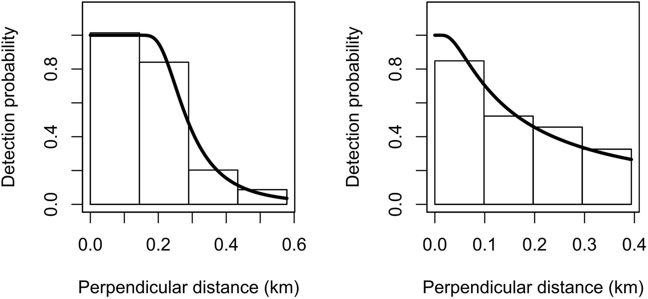
Figure 2. Fitted hazard-rate detection functions (solid lines) for Commerson’s dolphins (left) and Peale’s dolphins (right). The detection function is superimposed on a histogram of detection probabilities with bars scaled so that their areas match the area below the detection function.

Spatial Hurdle Models

The full Hurdle model yielded smooth term concurvity indices ranging between 0.32 and 0.99 (Supplementary Table 1). As a consequence, pairs of covariates with Pearson correlation coefficient (r) outside the interval including 0.5 and −0.5 were not considered together in the same model (Supplementary Table 2). Water stratification index was not correlated with any of the other covariates (−0.2 ≤ r ≤ 0.3), which instead were all correlated (−0.8 ≤ r ≤ −0.5 and 0.5 ≤ r ≤ 1), and thus not included together in the same sub-model variant (i.e., reduced Hurdle sub-models with different covariate structure). Although the Pearson correlation coefficient for the distance to the 100 m isobaths and water depth was equal to 0.4, a visual check through scatterplots suggested a substantial degree of correlation (not shown). This is reasonable as water depth increases so D100 decreases on the coastal side. DC, DRM, and DK were also positively correlated since kelp beds line the coast, and river mouths are also located along the coastline. We therefore applied model selection to five reduced sub-model variants that included the water stratification index in combination with each of the remaining covariates (Supplementary Table 3).

The variant including DRM and SI yielded the best fit for both PA and AB Commerson’s dolphin sub-models which explained 27.2 and 13.5% of the deviance, respectively (Supplementary Table 3). The covariate with the most pronounced effect on probability of presence was SI, which showed a U-shaped relationship with minimum values around 5 (Figures 3, 4). This relationship clearly showed that Commerson’s dolphins were associated with deep, well-stratified waters (SI > 5) as well as regions that experience very strong tidal mixing (SI < 2). Commerson’s dolphins were found close to tidal fronts as well as on both stratified and mixed sides. Both probability of presence and E(n|n > 0) (i.e., the estimated number of dolphins given presence) were inversely related to DRM, i.e., Commerson’s dolphins appeared to prefer to stay close to river mouths and tended to aggregate in such areas. Stratification index did not have an effect on estimated numbers of Commerson’s dolphins.

FIGURE 3

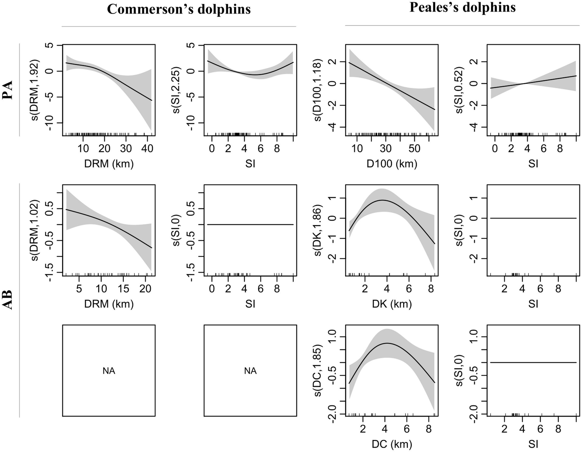
Figure 3. Smooth terms (s, linear predictor scale) of selected variants for presence-absence (PA) and numbers of dolphins given presence (AB) sub-models for Commerson’s and Peale’s dolphins. Smooth term effective degrees of freedom (edf) in brackets on the y-axis. Shaded area = 95% confidence intervals. Internal ticks show covariate values covered by the observations. DRM, distance to river mouth; SI, water stratification index; D100, distance to 100 m isobaths; DK, distance to kelp; DC, distance to coast.

FIGURE 4

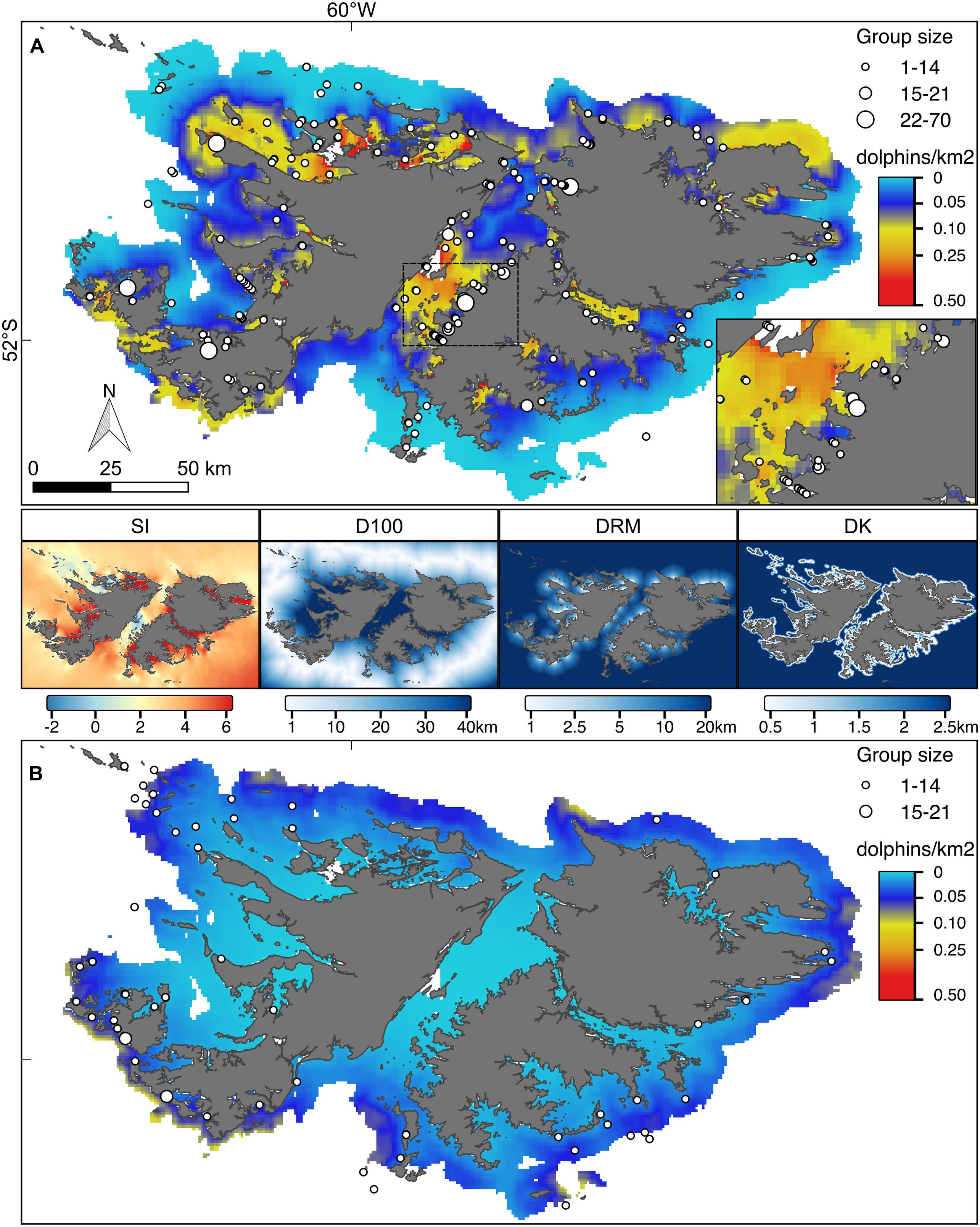
Figure 4. Hurdle model point estimates for the predicted number of Commerson’s and Peale’s dolphins (A and B, respectively). Superimposed locations represent the sightings collected during the aerial surveys conducted in 2017. Symbol size is proportional to the observed group sizes. Inset in (A) magnification of the central part of the Falkland Sound for Commerson’s dolphins. Both maps are reported on the same colour scale. The four maps in the middle show the covariate values: SI, water stratification index; D100, distance to 100 m isobaths; DRM, distance to main river mouth; DK, distance to kelp.

In addition to SI, the selected PA sub-model variant for Peale’s dolphins included D100 and explained 17.1% of the deviance (Supplementary Table 3). In contrast to Commerson’s dolphins, the AB sub-model included two variants with DK and DC explaining 38.1 and 33.3% of the deviance, respectively. Water stratification index had the lowest effect in the PA sub-model and no effect in the AB sub-model (Figures 3, 4). Probability of presence was inversely related to D100 and positively related to SI, while E(n|n > 0) for Peale’s dolphins showed a similar inversed U-shaped relationship with both DK and DC. Thus, Peale’s dolphins seemed to prefer offshore and well-stratified waters, but they tended to aggregate at approximately 2 km from kelp beds and coast. Since DK and DC belonged to two different variants, the degree of association of E(n|n > 0) for Peale’s dolphins with these two covariates differed, with covariates with highest δ_w having the highest degree of association. Thus, the E(n|n > 0) for Peale’s dolphins was more associated with DK (δ_w = 0.81) than with DC (δ_w = 0.17).

Concurvity indices for smooth terms within the selected sub-model variants for both dolphin species ranged between 0.08 and 0.31 (Supplementary Table1). QQ-plots and goodness-of-fit tests showed a satisfactory fit of the Hurdle model for Commerson’s dolphins (Kolmogorov–Smirnov test statistics = 0.14, p = 0.06) and a less satisfactory fit of that for Peale’s dolphins (Kolmogorov–Smirnov test statistics = 0.15, p = 0.03) (Supplementary Figure 2). Spatial correlation of Hurdle model residuals for Commerson’s dolphins decreased with distance while that for Peale’s showed a fluctuating pattern across the whole range of distances (Supplementary Figure 3). The proportion of the correlation values within −0.1 and 0.1 was 58% for Commerson’s and 70% for Peale’s dolphins.

Hurdle Model Predictions, Uncertainty, and Validation

According to the fitted Hurdle model, Commerson’s dolphins were found in all FI inshore waters (Figures 4–6). Larger numbers of Commerson’s dolphins were predicted for the central part of the Falkland Sound. In contrast, Peale’s dolphins were predicted to occur in more offshore waters and in lower densities (Figures 4–6). For both species predicted key areas matched the sighting locations of dolphins from the 2017 aerial surveys (SAERI unpublished data) which had covered 4,255 km in the entire inshore waters, with 195 and 55 groups of Commerson’s and Peale’s dolphins observed, respectively (Figures 4–6, Supplementary Figure 1). This finding suggests that the habitat model included an appropriate and sufficient set of relevant predictor variables to make effective predictions, and supports the assumption that the association between dolphins and habitat covariates remained consistent over time.

FIGURE 5

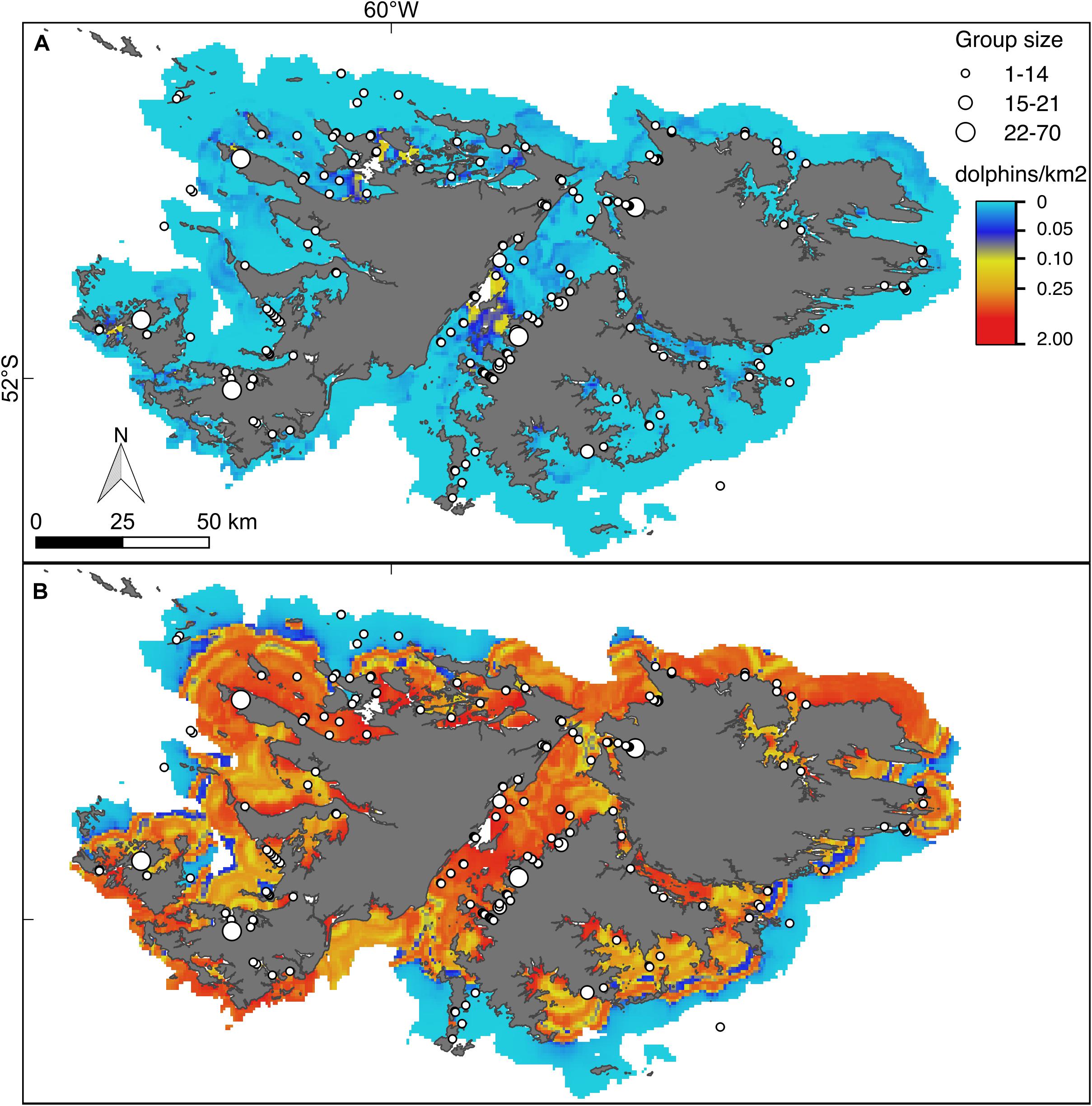
Figure 5. Hurdle model lower (A) and upper (B) bounds of the 95% confidence interval for the predicted density (dolphins/km²) of Commerson’s dolphins. For further explanation see Figure 4.

FIGURE 6

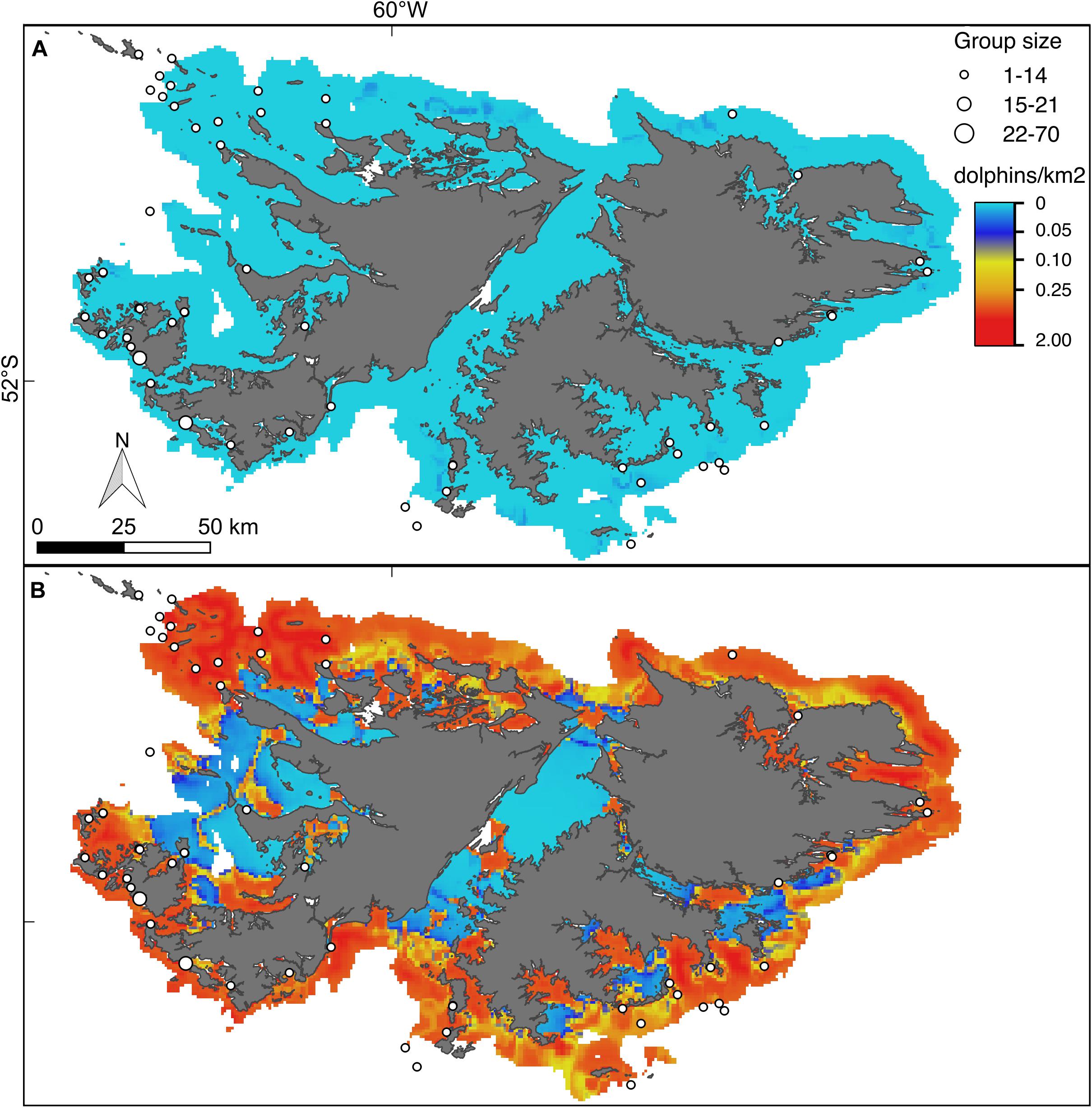
Figure 6. Hurdle model lower (A) and upper (B) bounds of the 95% confidence interval for the predicted density (dolphins/km²) of Peale’s dolphins. For further explanation see Figure 4.

Discussion

This study succeeded in generating robust spatial predictions from a spatially limited survey conducted over a short time period and extrapolating the distribution and habitat use of two dolphin species to cover the entire Falkland archipelago. Our results suggest that while some preferred habitat is shared, there is spatial niche separation between the two species.

Methodological Considerations

Representative sampling is an important consideration in modelling studies and requires some a priori knowledge of the species’ ecology. We were able to draw on ecological knowledge of each species from studies conducted in other parts of the species’ ranges (Garaffo et al., 2011; de Castro et al., 2013; Dellabianca et al., 2016; Heinrich et al., 2019) to guide the selection of potentially relevant environmental variables. The covariate ranges surveyed during the boat-based survey were representative of the overall FI inshore waters, thus allowing predictions within environmental space but extrapolation in geographic space.

Habitat modelling requires decisions about a trade-off between high-resolution data and model robustness. Where data are limited, model robustness can only be assured at the expense of data resolution. The resolution or grain size (e.g., segment area in our study) of the model should not be confused with the resolution of the prediction grid (e.g., grid cell area). The use of an offset term for grain size in the model allows for predictions of animal occurrence or relative abundance on higher resolution grid cells, while the underlying relationships are those originally fitted to the model grain size. Decreasing model resolution by taking large grain sizes also helps to reduce spatial autocorrelation in the response variable, which is a frequent problem in predictive habitat modelling (Guisan et al., 2007; Mannocci et al., 2017). Ideally one would like to know the best grain or segment size to ensure robustness and simultaneously maximise resolution (Mertes and Jetz, 2018). Splitting transects into segments can be a very tedious, time-consuming process that often requires the user to switch between different software packages. The newly developed “dshm” R-package greatly facilitates the splitting of transects into segments, the exploration of different grain sizes and the selection of a reasonable resolution to ensure model robustness.

This study presents five updates to the methodology currently used for predictive habitat modelling (Embling et al., 2010; Hammond et al., 2013; Dellabianca et al., 2016): (1) Use of zonal statistics: Predictor variables are usually derived by using a point-sampling approach, in which the covariate values associated with the chosen spatial unit (e.g., segment) are those sampled just below the unit centroids. This procedure might be inappropriate since habitat features at a small specific location might not be representative of the area where the animals were observed. We used a zonal-statistics approach in which the values of each predictor variable for a segment were derived as the median of all that covariate’s values available for that particular segment. Using the median rather than the mean decreased possible bias in covariate statistics for segments near the coastline. This is particularly important for heterogeneous environments, where covariate values might vary greatly over small spatial scales. (2) Use of buffered segments: Responsive movements are a common problem in boat-based surveys for cetaceans (Palka and Hammond, 2001) and can lead to biases in the detection probabilities (e.g., in our study both dolphin species showed strong attraction to the boat, leading to positive biases in the detection probabilities). Buffering the transect line by 1.5 km and using a zonal-statistics approach alleviated this attraction bias in our habitat modelling approach. The buffer size was chosen to reflect the range over which responsive movements were thought to occur. Thus, although the recorded spatial position of the animals might not represent their precise undisturbed position, the spatial integration of covariate values ensured representation of the natural habitat that the animals occurred in. (3) The binomial part of the Hurdle model allows zero inflation to be addressed. This is a common problem in animal surveys (Martin et al., 2005), and particularly so for rarely observed species (Welsh et al., 1996). Hurdle models are also ecologically sensible for scenarios where the processes driving the presence of a species differ from those affecting its abundance (Ridout et al., 1998). (4) Addressing GAM flexibility: The flexibility of the GAM framework is a “double-edged sword”: it enables one to model complex biological relationships but can also lead to overfitting (Morgan and Ridout, 2008). In this study the risk of overfitting was minimised by implementing a shrinkage version of cubic spline. (5) Stratum-specific bootstrapping: Model uncertainty was evaluated by using non-parametric bootstrapping with replacement, which is free from assumptions on parameter distributions (Fletcher et al., 2005). This approach, however, can be affected by fitting instabilities related to spatial gaps arising from resampling with replacement over the entire study area. We reduced such gaps by adopting a “stratified” approach in which resampling with replacement was limited to segments within the same stratum.

Predicting Distributions of Sympatric Dolphins

Our model predictions showed that Commerson’s and Peale’s dolphins used different key habitats around the FI with only some spatial overlap in distributions (Figures 4–6). Commerson’s dolphins were predicted to be most abundant in the central part of Falkland Sound, off the northern East Falkland coast as well as in the interior part of sounds and inlets around West and East Falkland. In contrast, Peale’s dolphins were predicted to occur mostly off the southern and north-western coasts of the Falkland archipelago. This difference in predicted spatial distributions resulted from the different modelled relationships that both species had with inshore habitat covariates. The environmental variables likely served as proxies for linked biological variables that could not be measured directly (such as the distribution or density of prey or predators) and might have reflected the differences in species-specific physiological and ecological responses (Kiszka et al., 2015; de Thoisy et al., 2016).

Probability of presence of Commerson’s dolphins appeared to be linked to the water SI with areas of very low SI (e.g., Falkland Sound) or very high SI (e.g., northern West Falkland, most FI inlets) being those where Commerson’s dolphins were most likely to occur (Figure 4). This suggests that Commerson’s dolphins preferred to be close to tidal fronts as well as stay on the mixed or stratified sides. The importance of tidal fronts to the distribution of Commerson’s dolphins has also been suggested for the Argentinian coast (Dellabianca et al., 2016). In contrast to presence, Commerson’s dolphin abundance seemed to be mostly linked to distance to rivers with the highest numbers occurring in upper inlets, and close to river mouths. Such preference for nearshore neritic environments with strong tidal influence and estuarine zones is a defining feature for all species in the genus Cephalorhynchus (Heinrich et al., 2010; de Castro et al., 2013; Heinrich et al., 2019).

Presence of Peale’s dolphins was mostly associated with D100, with the highest probability of observing the species close to the 100 m isobaths, i.e., shelf-waters further offshore. Although occurrence was predicted to be higher in deeper and well-stratified shelf waters, Peale’s dolphins also tended to be more numerous in shallower waters close to the coast and near to kelp as shown by the importance of both DK and DC in the abundance model and the resulting predicted distribution (Figures 3, 4). Such overall plasticity in occurrence has now emerged as a feature consistent for Peale’s dolphins across their entire distributional range (Dellabianca et al., 2016; Heinrich et al., 2019; this study). Peale’s dolphins’ reliance on nearshore habitat, at least during summer, is well documented from southern Argentina (De Haro and Iñiguez, 1997), with kelp forests thought to represent important feeding grounds (Schiavini et al., 1997; Viddi and Lescrauwaet, 2005; Riccialdelli et al., 2010). The low number of Peale’s dolphin sightings affected the model goodness-of-fit (p-value near the 5% threshold, Supplementary Figure 2). Despite these limitations the resulting predicted spatial distribution was well matched by sightings from the independent aerial survey suggesting that the model predictions succeeded in capturing the dolphins’ overall habitat preference.

Although Commerson’s and Peale’s dolphins are fully sympatric across their South Atlantic range, our predicted distribution maps and other large-scale modelling studies (Dellabianca et al., 2016) indicate fine-scale habitat partitioning between the two species. Strategies that enable sympatric species to co-exist include spatial or temporal differences in habitat use, dietary divergence and specialisation, as well as differences in activity patterns and socially mediated behaviours (Begon et al., 2006). Future research into niche partitioning of these two species should therefore focus on investigating ranging patterns, site fidelity, social interactions (e.g., using individual identification studies; e.g., Parra, 2006; Coscarella et al., 2011) and establishing diet and trophic niche overlap (using stable isotope or fatty acid analyses; e.g., Querouil et al., 2013; Giménez et al., 2018). The predicted distribution maps from this study should prove helpful to identify suitable FI study areas for such intensive, focal research endeavours.

Conservation and Management Relevance

The most recent Falkland Islands Species Action Plan for Cetaceans (2008–2018) identifies a range of suspected and known threats to the marine ecosystem on the shelf around the FI, including pollution, bycatch, vessel traffic and climate change, and highlights novel and expanding activities with the potential for harmful interactions such as aquaculture, tourism and commercial fishing (Otley, 2008). Identifying potential areas of importance for these dolphin species as well as their overlap with human activities should serve as a guide for future research efforts and the current FI marine spatial planning activities.

The underlying data for such studies is, however, often very hard to obtain, especially as information from a range of species is needed to enable focussed management and conservation efforts. One can argue that meso and top predators often forage in aggregations with other species (hotspots) and that therefore the use of data from sentinel species are enough, but on smaller scales, as in coastal waters, niche separation might indicate reliance on different prey and/or areas. Relevant high-resolution data are therefore necessary to resolve such differences. Remote tracking technologies have enabled us to collect high-resolution information about movements and foraging behaviour, but while such data can provide an unprecedented amount of detail, studies are usually limited to one species, low numbers or are hampered by a lack of concurrent data in case of multi-species approaches (Baylis et al., 2019).

We have shown a practical and cost-effective approach using a spatially limited dataset to estimate multi-species distribution patterns. We have demonstrated the robustness of this method by comparing the patterns with sightings from another survey. The methodology and software implementations provided here can be easily applied to transect survey data of other mobile marine and terrestrial taxa where the area of interest is representative of but larger than the area surveyed. This will help us to address the challenges ahead in conservation and management of the marine environment.

Data Availability Statement

The datasets generated for this study are available on request to the corresponding author.

Ethics StaTement

The animal study was reviewed and approved by University of St Andrews, School of Biology Animal Ethics Committee.

Author Contributions

FF undertook the statistical modelling and GIS analysis. CB assisted with the GIS analysis. SS assisted with the statistical modelling. LB assisted with some of the covariate generation. GM and SH designed the study and collected the 2014 data. MC led the 2017 aerial surveys that provided the independent dataset for corroboration of predicted distributions. FF, SH, SS, and LB wrote the manuscript. All authors commented on the analyses and the final manuscript and approved the final manuscript to be published.

Funding

The field work was funded by the Darwin Initiative UK Overseas Territories Challenge Fund Project “Inshore Cetaceans of the Falkland Islands” (Project Ref: EIDCF019, administered jointly by Falklands Conservation & Mr. Grant Munro), and Darwin Plus: Overseas Territories Environment and Climate Fund Project “Dolphins of the kelp: Data priorities for Falkland’s inshore cetaceans” (Project Ref: DPLUS042, administered by SAERI).

Conflict of Interest

Grant Munro was employed by company Austral Biodiversity Ltd.

The remaining authors declare that the research was conducted in the absence of any commercial or financial relationships that could be construed as a potential conflict of interest.

Acknowledgements

We wish to thank all the Falkland Conservation volunteers who assisted with the data collection, in particular Miss Iris Thomsen for collating the 2014 survey data, and Michael and Jeanette Clarke of the vessel “Condor”. We also want to thank the Falkland Island (FI) Government for providing the research permit for the 2014 survey. We thank the SAERI IMS-GIS Data Centre for providing access to the digitised FI coastline and some of the kelp beds. We also thank Prof David L. Borchers at CREEM for the stimulating discussions about aspects of the modelling approach. We are grateful to the two reviewers for their constructive comments that improved the original manuscript.

Supplementary Material

The Supplementary Material for this article can be found online at: https://www.frontiersin.org/articles/10.3389/fmars.2020.00277/full#supplementary-material

Footnotes

1. ^ https://github.com/FilippoFranchini/dshm

References

Acha, E. M., Mianzan, H. W., Guerrero, R. A., Favero, M., and Bava, J. (2004). Marine fronts at the continental shelves of austral South America: physical and ecological processes. J. Mar. Syst. 44, 83–105. doi: 10.1016/j.jmarsys.2003.09.005

CrossRef Full Text | Google Scholar

Augé, A. A., Dias, M. P., Lascelles, B., Baylis, A. M., Black, A., Boersma, P. D., et al. (2018). Framework for mapping key areas for marine megafauna to inform marine spatial planning: the Falkland Islands case study. Mar. Policy 92, 61–72. doi: 10.1016/j.marpol.2018.02.017

CrossRef Full Text | Google Scholar

Austin, M. P., Nicholls, A. O., and Margules, C. R. (1990). Measurement of the realized qualitative niche: environmental niches of five eucalyptus species. Ecol. Monogr. 60, 161–177. doi: 10.2307/1943043

CrossRef Full Text | Google Scholar

Barragán-Barrera, D. C., do Amaral, K. B., Chávez-Carreño, P. A., Farías-Curtidor, N., Lancheros-Neva, R., Botero-Acosta, N., et al. (2019). Ecological niche modeling of three species of stenella dolphins in the caribbean basin, with application to the seaflower biosphere reserve. Front. Mar. Sci. 6:10. doi: 10.3389/fmars.2019.00010

CrossRef Full Text | Google Scholar

Baylis, A. M. M., Tierney, M., Orben, R. A., Warwick-Evans, V., Wakefield, E., Grecian, W. J., et al. (2019). Important at-sea areas of colonial breeding marine predators on the southern patagonian shelf. Sci. Rep. 9:8517. doi: 10.1038/s41598-019-44695-1

PubMed Abstract | CrossRef Full Text | Google Scholar

Begon, M., Townsend, C. R., and Harper, J. L. (2006). Ecology: From Individuals to Ecosystems, 5th Edn. Oxford: Blackwell.

Google Scholar

Bost, C.-A., Cotté, C., Bailleul, F., Cherel, Y., Charrassin, J.-B., Guinet, C., et al. (2009). The importance of oceanographic fronts to marine birds and mammals of the southern oceans. J. Mar. Syst. 78, 363–376. doi: 10.1016/j.jmarsys.2008.11.022

CrossRef Full Text | Google Scholar

Buckland, S. T., Anderson, D. R., Burnham, K. P., Laake, J. L., Borchers, D. L., and Thomas, L. (2001). Introduction to Distance Sampling: Estimating Abundance of Biological Populations. New York: Oxford University Press.

Google Scholar

Cipriano, F. (2018). “Peale’s Dolphin: Lagenorhynchus australis,” in Encyclopedia of Marine Mammals, 3 Edn, eds B. Würsig, J. G. M. Thewissen, and K. M. Kovacs (Academic Press), 698–701.

Google Scholar

Coscarella, M. A., Gowans, S., Pedraza, S. N., and Crespo, E. A. (2011). Influence of body size and ranging patterns on delphinid sociality: associations among Commerson’s dolphins. J. Mammal. 92, 544–551. doi: 10.1644/10-mamm-a-029.1

CrossRef Full Text | Google Scholar

Davis, R. W., Ortega-Ortiz, J. G., Ribic, C. A., Evans, W. E., Biggs, D. C., Ressler, P. H., et al. (2002). Cetacean habitat in the northern oceanic Gulf of Mexico. Deep Sea Res. I Oceanogr. Res. Pap. 49, 121–142. doi: 10.1016/s0967-0637(01)00035-8

CrossRef Full Text | Google Scholar

de Castro, R. L., Dans, S. L., Coscarella, M. A., and Crespo, E. A. (2013). Living in an estuary: commerson’s dolphin (Cephalorhynchus commersonii (Lacépède, 1804)), habitat use and behavioural pattern at the Santa Cruz River, Patagonia, Argentina. Latin Am. J. Aquat. Res. 41, 985–991. doi: 10.3856/vol41-issue5-fulltext-17

CrossRef Full Text | Google Scholar

De Haro, J. C., and Iñiguez, M. (1997). Ecology and behavior of the Peale’s dolphin, Lagenorhynchus australis (Peale, 1848), at Cabo Virgenes (52 degrees 30’ S., 68 degrees 28’ W.), in Patagonia, Argentina. Rep. Int.Whaling Commission 47, 723–727.

Google Scholar

de Thoisy, B., Fayad, I., Clément, L., Barrioz, S., Poirier, E., and Gond, V. (2016). Predators, prey and habitat structure: can key conservation areas and early signs of population collapse be detected in neotropical forests? PLoS One 11:e0165362. doi: 10.1371/journal.pone.0165362

PubMed Abstract | CrossRef Full Text | Google Scholar

Dellabianca, N. A., Pierce, G. J., Rey, A. R., Scioscia, G., Miller, D. L., Torres, M. A., et al. (2016). Spatial models of abundance and habitat preferences of Commerson’s and Peale’s dolphin in Southern Patagonian waters. PLoS One 11:e0163441. doi: 10.1371/journal.pone.0163441

CrossRef Full Text | Google Scholar

Dellabianca, N. A., Scioscia, G., Schiavini, A., and Rey, A. R. (2012). Occurrence of hourglass dolphin (Lagenorhynchus cruciger) and habitat characteristics along the Patagonian Shelf and the Atlantic Ocean sector of the Southern Ocean. Polar Biol. 35, 1921–1927. doi: 10.1007/s00300-012-1217-0

CrossRef Full Text | Google Scholar

Egbert, G. D., and Erofeeva, S. Y. (2002). Efficient inverse modeling of barotropic ocean tides. J. Atmos. Ocean. Technol. 19, 183–204. doi: 10.1175/1520-0426(2002)019<0183:eimobo>2.0.co;2

CrossRef Full Text | Google Scholar

Embling, C. B., Gillibrand, P. A., Gordon, J., Shrimpton, J., Stevick, P. T., and Hammond, P. S. (2010). Using habitat models to identify suitable sites for marine protected areas for harbour porpoises (Phocoena phocoena). Biol. Conserv. 143, 267–279. doi: 10.1016/j.biocon.2009.09.005

CrossRef Full Text | Google Scholar

Fletcher, D., MacKenzie, D., and Villouta, E. (2005). Modelling skewed data with many zeros: a simple approach combining ordinary and logistic regression. Environ. Ecol. Stat. 12, 45–54. doi: 10.1007/s10651-005-6817-1

CrossRef Full Text | Google Scholar

Garaffo, G. V., Dans, S. L., Pedraza, S. N., Degrati, M., Schiavini, A., González, R., et al. (2011). Modeling habitat use for dusky dolphin and Commerson’s dolphin in Patagonia. Mar. Ecol. Prog. Ser. 421, 217–227. doi: 10.1371/journal.pone.0126182

PubMed Abstract | CrossRef Full Text | Google Scholar

Gillespie, D. M., Leaper, R., Gordon, J. C. D., and Macleod, K. (2010). A semi-automated, integrated, data collection system for line transect surveys. J. Cetacean Res. Manage. 11, 217–227.

Google Scholar

Giménez, J., Cañadas, A., Ramírez, F., Afán, I., García-Tiscar, S., Fernández-Maldonado, C., et al. (2018). Living apart together: niche partitioning among Alboran Sea cetaceans. Ecol. Indic. 95, 32–40. doi: 10.1016/j.ecolind.2018.07.020

CrossRef Full Text | Google Scholar

Guisan, A., Graham, C. H., Elith, J., Huettmann, F., and Group, N. S. D. M. (2007). Sensitivity of predictive species distribution models to change in grain size. Divers. Distrib. 13, 332–340. doi: 10.1111/j.1472-4642.2007.00342.x

CrossRef Full Text | Google Scholar

Guisan, A., Tingley, R., Baumgartner, J. B., Naujokaitis-Lewis, I., Sutcliffe, P. R., Tulloch, A. I., et al. (2013). Predicting species distributions for conservation decisions. Ecol. Lett. 16, 1424–1435. doi: 10.1111/ele.12189

PubMed Abstract | CrossRef Full Text | Google Scholar

Guisan, A., and Zimmermann, N. E. (2000). Predictive habitat distribution models in ecology. Ecol. Model. 135, 147–186. doi: 10.1016/s0304-3800(00)00354-9

CrossRef Full Text | Google Scholar

Hammond, P. S., Macleod, K., Berggren, P., Borchers, D. L., Burt, L., Cañadas, A., et al. (2013). Cetacean abundance and distribution in European Atlantic shelf waters to inform conservation and management. Biol. Conserv. 164, 107–122. doi: 10.1016/j.biocon.2013.04.010

CrossRef Full Text | Google Scholar

Heinrich, S., Elwen, S., and Bräger, S. (2010). “Patterns of sympatry in Lagenorhynchus and Cephalorhynchus: dolphins in different habitats,” in The Dusky Dolphin, eds W. Würsig and B. Würsig (Elsevier), 313–332. doi: 10.1016/b978-0-12-373723-6.00015-1

CrossRef Full Text | Google Scholar

Heinrich, S., Genov, T., Fuentes Riquelme, M., and Hammond, P. S. (2019). Fine scale habitat partitioning of Chilean and Peale’s dolphins and their overlap with aquaculuture. Aquat. Conserv. Mar. Freshw. Ecosyst. 29, 212–226. doi: 10.1002/aqc.3153

CrossRef Full Text | Google Scholar

Hill, A., Brown, J., Fernand, L., Holt, J., Horsburgh, K., Proctor, R., et al. (2008). Thermohaline circulation of shallow tidal seas. Geophys. Res. Lett. 35:L11605.

Google Scholar

Kiszka, J. J., Heithaus, M. R., and Wirsing, A. J. (2015). Behavioural drivers of the ecological roles and importance of marine mammals. Mar. Ecol. Prog. Ser. 523, 267–281. doi: 10.3354/meps11180

CrossRef Full Text | Google Scholar

Mannocci, L., Boustany, A. M., Roberts, J. J., Palacios, D. M., Dunn, D. C., Halpin, P. N., et al. (2017). Temporal resolutions in species distribution models of highly mobile marine animals: recommendations for ecologists and managers. Divers. Distrib. 23, 1098–1109. doi: 10.1111/ddi.12609

CrossRef Full Text | Google Scholar

Mannocci, L., Laran, S., Monestiez, P., Dorémus, G., Van Canneyt, O., Watremez, P., et al. (2014). Predicting top predator habitats in the Southwest Indian Ocean. Ecography 37, 261–278. doi: 10.1111/j.1600-0587.2013.00317.x

CrossRef Full Text | Google Scholar

Martin, T. G., Wintle, B. A., Rhodes, J. R., Kuhnert, P. M., Field, S. A., Low-Choy, S. J., et al. (2005). Zero tolerance ecology: improving ecological inference by modelling the source of zero observations. Ecol. Lett. 8, 1235–1246. doi: 10.1111/j.1461-0248.2005.00826.x

PubMed Abstract | CrossRef Full Text | Google Scholar

Mertes, K., and Jetz, W. (2018). Disentangling scale dependencies in species environmental niches and distributions. Ecography 41, 1604–1615. doi: 10.1111/ecog.02871

CrossRef Full Text | Google Scholar

Morgan, B. J., and Ridout, M. S. (2008). A new mixture model for capture heterogeneity. J. R. Stat. Soc. Ser. C 57, 433–446. doi: 10.1111/j.1467-9876.2008.00620.x

CrossRef Full Text | Google Scholar

Otley, H. (2008). Falkland Islands Species Action Plan for Cetaceans 2008-2018. Stanley: The Environmental Planning Department.

Google Scholar

Palka, D., and Hammond, P. (2001). Accounting for responsive movement in line transect estimates of abundance. Can. J. Fish. Aquat. Sci. 58, 777–787. doi: 10.1139/f01-024

CrossRef Full Text | Google Scholar

Parra, G. J. (2006). Resource partitioning in sympatric delphinids: space use and habitat preferences of Australian snubfin and Indo-Pacific humpback dolphins. J. Anim. Ecol. 75, 862–874. doi: 10.1111/j.1365-2656.2006.01104.x

PubMed Abstract | CrossRef Full Text | Google Scholar

Qgis Development Team (2017). QGIS Geographic Information System. Beaverton: Open Source Geospatial Foundation.

Google Scholar

Querouil, S., Kiszka, J., Cordeiro, A., Cascão, I., Freitas, L., Dinis, A., et al. (2013). Investigating stock structure and trophic relationships among island-associated dolphins in the oceanic waters of the North Atlantic using fatty acid and stable isotope analyses. Mar. Biol. 160, 1325–1337. doi: 10.1007/s00227-013-2184-x

CrossRef Full Text | Google Scholar

Ramsay, T. O., Burnett, R. T., and Krewski, D. (2003). The effect of concurvity in generalized additive models linking mortality to ambient particulate matter. Epidemiology 14, 18–23. doi: 10.1097/00001648-200301000-00009

PubMed Abstract | CrossRef Full Text | Google Scholar

Riccialdelli, L., Newsome, S. D., Fogel, M. L., and Goodall, R. N. P. (2010). Isotopic assessment of prey and habitat preferences of a cetacean community in the southwestern South Atlantic Ocean. Mar. Ecol. Prog. Ser. 418, 235–248. doi: 10.3354/meps08826

CrossRef Full Text | Google Scholar

Ridout, M., Demétrio, C. G. B., and Hinde, J. (1998). “Models for count data with many zeros,” in Proceedings of the XIXth International Biometric Conference, (Cape Town), 179–192.

Google Scholar

Schiavini, A. C. M., Goodall, R. N. P., Lescrauwaet, A.-K., and Koen Alonso, M. (1997). Food habits of Peale’s dolphin, Lagenorhynchus australis, review and new information. Int. Whaling Commission Rep. 47, 827–834.

Google Scholar

Simpson, J., and Hunter, J. (1974). Fronts in the Irish sea. Nature 250:404. doi: 10.1038/250404a0

CrossRef Full Text | Google Scholar

Thomas, L., Buckland, S. T., Rexstad, E. A., Laake, J. L., Strindberg, S., Hedley, S. L., et al. (2010). Distance software: design and analysis of distance sampling surveys for estimating population size. J. Appl. Ecol. 47, 5–14. doi: 10.1111/j.1365-2664.2009.01737.x

PubMed Abstract | CrossRef Full Text | Google Scholar

Thomsen, I. J. T. (2013). Designing a Pilot Line Transect Survey for Inshore Cetaceans in the Falkland Islands. MRes dissertation, University of St Andrews, St Andrews.

Google Scholar

Thomsen, I. J. T. (2014). Results from the Pilot Line Transect Survey for Inshore Cetaceans in the Falkland Islands and designing a Full Falkland Island Line Transect Survey for Inshore Cetaceans. St Andrews: University of St Andrews.

Google Scholar

van Etten, J. (2017). R Package gdistance: distances and routes on geographical grids. J. Stat. Softw. 76, 1–21. doi: 10.18637/jss.v076.i13

CrossRef Full Text | Google Scholar

Viddi, F. A., and Lescrauwaet, A. (2005). Insights on habitat selection and behavioural patterns of Peale’s dolphins (Lagenorhynchus australis) in the Strait of Magellan, Southern Chile. Aquat. Mamm. 31, 176–183. doi: 10.1578/am.31.2.2005.176

CrossRef Full Text | Google Scholar

Weatherall, P., Marks, K. M., Jakobsson, M., Schmitt, T., Tani, S., Arndt, J. E., et al. (2015). A new digital bathymetric model of the world’s oceans. Earth Space Sci. 2, 331–345. doi: 10.1002/2015ea000107

CrossRef Full Text | Google Scholar

Welsh, A. H., Cunningham, R. B., Donnelly, C., and Lindenmayer, D. B. (1996). Modelling the abundance of rare species: statistical models for counts with extra zeros. Ecol. Model. 88, 297–308. doi: 10.1016/0304-3800(95)00113-1

CrossRef Full Text | Google Scholar