Biogeography of Micronekton Assemblages in the Natural Park of the Coral Sea

Introduction

Marine biodiversity is predicted to decrease in the coming decades on a global scale (Garcia Molinos et al., 2016; Worm and Lotze, 2016) with human activities, such as fishing, pollution, and habitat perturbation, identified as key drivers of this decrease (Lotze et al., 2006; Diaz et al., 2019). Climate change, another main threat to marine diversity, is causing large modifications in species spatial distribution (Cheung et al., 2009; Pecl et al., 2017; Hillebrand et al., 2018; Lotze et al., 2019) and, therefore, induces local changes in assemblage composition (Dornelas et al., 2014).

This global loss of biodiversity is threatening ecosystem functioning as well as the services it provides, which are essential for human well-being (Worm et al., 2006; Beaumont et al., 2007; Cardinale et al., 2012; Hannah et al., 2013). Marine protected areas (MPAs) and large-scale MPAs have been identified as key species-conservation tools (Ehler and Douvere, 2009; Christie et al., 2017; Davidson and Dulvy, 2017) as well as to mitigate the effects of climate change (Roberts et al., 2017). In the vast pelagic domain, MPAs have been offered as tool to protect migratory species (Davies et al., 2012). However, it has been emphasized that, at the global scale, the current level of protection of marine ecosystems spatially mismatched the important regions in terms of diversity; for instance, main diversity hot spots are mostly outside protected areas (Lindegren et al., 2018). This relatively inefficient global management could be explained by the knowledge gap in marine species ecology (especially environmental drivers of their spatial distribution) and species interactions (trophic or others) (Dornelas et al., 2014). Therefore, climate change impacts could be mitigated by improving the understanding of species optimal environmental conditions and by including this in global strategic frameworks for management and conservation (Pecl et al., 2017; Glover et al., 2018). However, this should not be limited to a small number of emblematic species, as is often the case, but should aim at encompassing the whole species assemblages (Fisher et al., 2011).

In pelagic ecosystems, mid-trophic-level organisms (MTLOs), also referred to as micronekton, include crustaceans, mollusks, gelatinous organisms, and fish with size ranging from 1 to 20 cm long (e.g., Bertrand et al., 2002; Young et al., 2015). Micronekton species play a central role in the pelagic ecosystem as food of predators, including commercially targeted species, such as tuna (Bertrand et al., 2002; Olson et al., 2014; Duffy et al., 2017), and emblematic marine species, such as seabirds, cetaceans, and sharks (Lambert et al., 2014; Miller et al., 2018). Hence, micronekton diversity directly impacts predators’ diet (Duffy et al., 2017; Portner et al., 2017). Micronekton perform daily migrations between the surface layer (0–200 m), where they stay during the night, and the mesopelagic layer (200–1000 m), where they stay during the day to avoid visual predation. This vertical migration largely participates in the downward flux of nutrients and particulate organic matter via respiration and excretion processes (Hidaka et al., 2001; Ariza et al., 2015; Drazen and Sutton, 2017). This diel vertical migration pattern (DVM) is observed in the world’s oceans (Bianchi and Mislan, 2016; Klevjer et al., 2016) and is performed by a large majority of species (75% of organisms in the southwest Pacific according to Receveur et al., 2019). Despite their important role, the dynamic of micronektonic species in their environment is still poorly understood (St. John et al., 2016; Hidalgo and Browman, 2019). In particular, species vertical behavior (e.g., percentage of individuals performing DVM) is one knowledge gap to solve in order to include micronekton in biogeochemical models of the carbon cycle (Aumont et al., 2018). The large intrinsic micronekton diversity (Olivar et al., 2017) and the poor observation level complicate a complete understanding of the mesopelagic species ecology. Indeed, each micronektonic species has a specific habitat that is challenging to identify (Duffy et al., 2017).

In the New Caledonian Exclusive Economic Zone (EEZ), located in the Coral Sea at the southwestern edge of the Pacific Ocean, top predator diet studies (Young et al., 2010; Allain et al., 2012; Olson et al., 2014; Williams et al., 2014) and trawl data analyses (Grandperrin et al., 1999; Young et al., 2011; Menkes et al., 2015) reveal a high diversity of micronekton organisms (Payri et al., 2019). This high diversity also supports high richness of top predator species (Ceccarelli et al., 2013; Laran et al., 2016) with the presence of several species of cetaceans (Mannocci et al., 2014; Garrigue et al., 2015), sharks (Bakker et al., 2017; Boussarie et al., 2018), seabirds (Borsa et al., 2014, 2015; Weimerskirch et al., 2017), and tuna (Roger, 1976, 1986). Moreover, the seabed topography is complex around New Caledonia (Gardes et al., 2014) with the presence of three ridges (about 1000 m depth), numerous seamounts with a high shape diversity (summit depth from 1000 to 10 m), one trench (about 6000 m depth), and some sedimentary basins (about 3000 m depth) (Figure 1). Such complex bathymetry offers a large number of habitats that could enhance micronekton diversity and biomass as demonstrated for seamounts (Morato et al., 2010; Drazen et al., 2011) or ridges (Hudson et al., 2014; Laptikhovsky et al., 2017) for example.

FIGURE 1

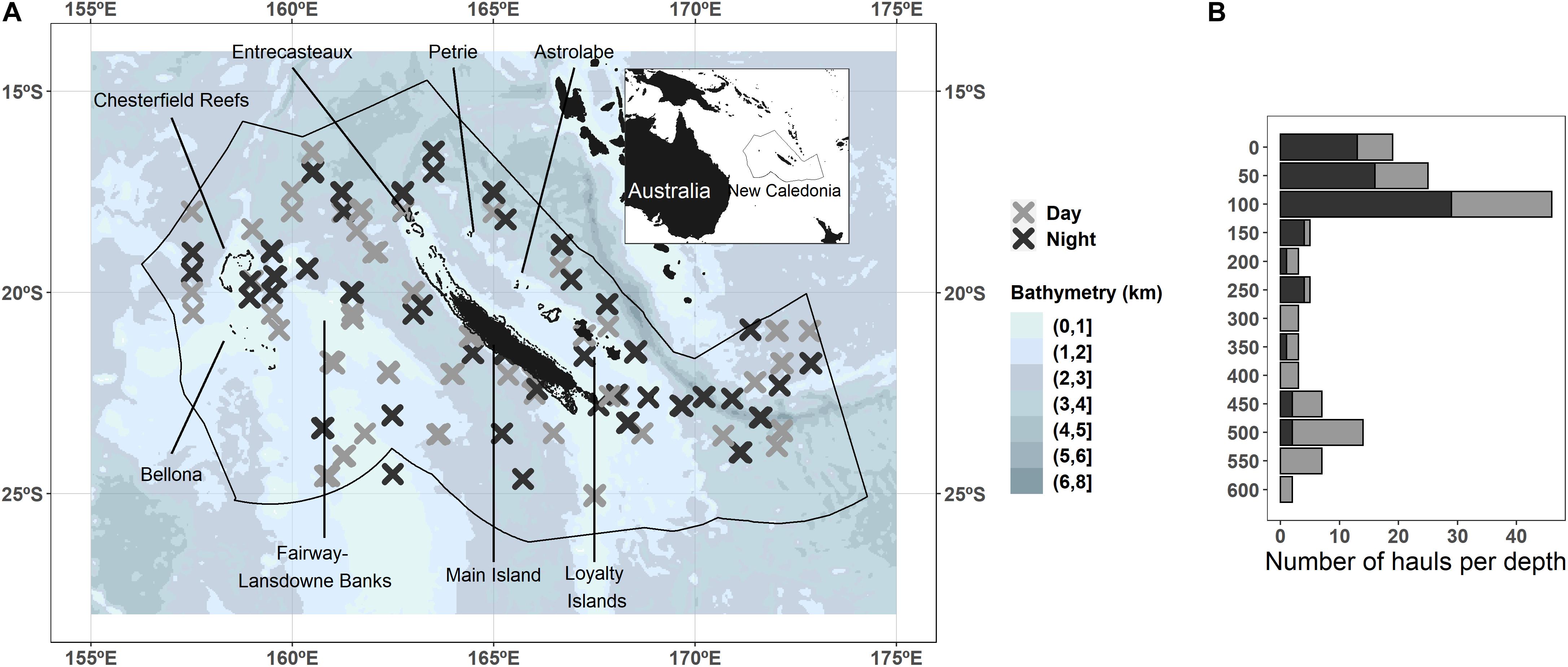
Figure 1. Trawl hauls’ spatial position colored by the moment of the day (gray and dark crosses) in the New Caledonian Exclusive Economic Zone. The background blue colors represent the seabed depth (where lighter colors are shallower). Note that hauls from two cruises in the northern part partially overlap, and for visualization purposes haul positions have been shifted by 0.5° to the north (A). The number of hauls per depth colored by the moment of the day (B).

The Natural Park of the Coral Sea was recently created, covering the entire oceanic waters of New Caledonia (Decree 2014-1063/GNC). To develop the management plan of the park, there is an important need for robust scientific information on the productivity and functioning of this pelagic ecosystem, including micronekton dynamics and role in food webs (Ceccarelli et al., 2013; Gardes et al., 2014). Additional information on micronekton assemblages and diversity will contribute to designing the Natural Park management plan, accounting for the conservation of the food stock of all top predators.

In this context, the large diversity of predators and micronekton makes the New Caledonian EEZ a good case study to understand the pelagic ecosystem functioning and to implement a management tool. The present study focuses especially on micronekton assemblage diversity, one of the most poorly understood links in pelagic ecosystems (St. John et al., 2016; Hidalgo and Browman, 2019). Using data from 141 mesopelagic hauls conducted in the New Caledonian EEZ in 2011–2016, we applied region of common profile (RCP) methodology to quantitatively characterize the micronektonic assemblages, to identify the environmental conditions influencing those assemblages, and to determine their spatial distribution. RCP also allowed the description of the vertical distribution of the most abundant species as well as their spatial distribution.

Materials and Methods

Sample Collection

We gathered data from five cruises (Nectalis 1 to 5,¹ ‘N1’ to ‘N5’ hereafter; Supplementary Table S1) on board the R/V Alis in the New Caledonian EEZ, covering the area between 156°E–175°E and 14°S–27°S over the period 2011 to 2016 (Figure 1A). The sampling strategy was constrained by the availability of the vessel, the cyclonic season, the duration of the cruise, the small size of the vessel (28 m), and the number of hours worked by the crew. The sampling strategy of the five cruises aimed primarily at covering spatially the whole EEZ of New Caledonia. N1 and N2 covered the northern region; N3, N4, covered the southwest; and N5 covered the southeast (Supplementary Figure S1). The second objective was also to consider seasonal variability with N1 covering the cold season and N2 covering the warm season in the northern area. It was originally planned to do the same in the southern part of the EEZ with N3 carried out during the warm season, and N4 was supposed to be conducted during the cold season. However, the availability of the vessel allowed us to carry out N4 at the transition period between the two seasons only. Moreover, N4 was interrupted after a few days because of an engine failure. N5 was meant to reproduce N4 the following year, but the vessel was available only during the warm season, and considering the weather conditions at the time, it was decided to explore the southeast instead of the southwest area. These successive constraints explained some lack of systematic sampling of space and time. Sampling stations were distributed evenly along the tracks and lasted 5–7 h each (Supplementary Figure S1). The sampling was conducted as much as possible to balance the day and night and the depth according to the ship’s arrival time at the station and avoiding dawn and dusk when micronekton migrates. At each station one, two, or three trawl hauls were conducted within 4 h at different depths. Depth sampled was selected according to an echosounder signal targeting the layers where the acoustic signal was the strongest. Given all these limitations, the data sampling remains rather well balanced (Figure 1B and Supplementary Table S2).

Acoustic data were recorded continuously during cruises using an EK60 echosounder (SIMRAD Kongsberg Maritime AS, Horten, Norway) connected to four split-beam transducers at 38, 70, 120, and 200 kHz. Micronekton organisms were sampled at each station with a mid-water trawl with a 10-mm mesh. Vertical and horizontal mouth openings of about 10 m were monitored with trawl opening sensors (Scanmar, Åsgårdstrand, Norway). Horizontal tows were conducted to target aggregations visually detected with the EK60 echosounder during both day and night periods (Figure 1B). Once the net was stabilized at the echo depth, based on Scanmar depth-positioning information, it was towed for about 30 min with a vessel speed around 3–4 knots. One to three hauls were conducted at each station at depths varying between 10 and 590 m during the day and between 10 and 520 m during the night. Organisms collected were quickly sorted by broad taxon (e.g., Crustacea, Actinopterygii, Cephalopoda) on board the vessel and immediately frozen at −20°C.

In the laboratory, specimens were defrosted and identified to the lowest possible taxon based on morphologic criteria and using identification keys. Identified specimens were counted and weighed. Gelatinous organisms were removed from analysis as accurate counts and weights cannot be recorded due to the fragility of those organisms and their high percentage of water. Indeed, they are easily damaged during trawling and freezing, limiting the accuracy of identification. Individuals from colonies got separated during trawling, making the counting of organisms imprecise, and thawing made them lose their water content such that weighting was non-representative of the fresh wet weight.

The volume filtered by the net was calculated as V=SD with S=hv and $D=2R{\tan }^{-1}(\sqrt{a/(1-a)})$. The intermediate a was calculated as follows:

$$a={[\sin ((la{t}_2-la{t}_1)/2)]}^2+\cos (la{t}_1)$$

$$\cos (la{t}_2){[\sin ((lo{n}_2-lo{n}_1)/2)]}^2,$$

where V is the volume filtered (m³); S is the net mouth opening (m²); D is the distance covered by the trawl (m); h and v are the net horizontal and vertical mouth openings (m); R = 6371 is the Earth’s radius (km); and lat₁, lat₂, lon₁, and lon₂ are the latitude and longitude of the start and end of the set at the chosen depth (radian). More details about N1 and N2 are given in Menkes et al. (2015).

Environmental Variables

Environmental variables were selected to explore the sampling conditions of micronekton assemblages (Table 1). For each haul, environmental data were extracted at the date and position of the sample.

TABLE 1

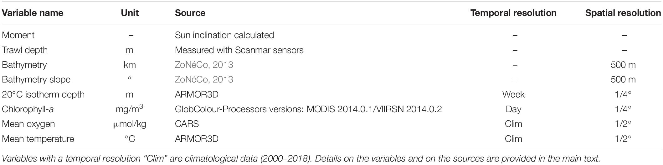
Table 1. Summary of environmental variables with unit, source, and resolutions.

Sun inclination was calculated as a function of spatial position and date (Michalsky, 1988; Blanc and Wald, 2012), and hauls were categorized into “Day” and “Night” periods (negative values corresponding to Night and positive values to Day). Bathymetry data was extracted from the ZoNéCo database at a 500 m spatial resolution (ZoNéCo, 2013),² and the slope of the bottom was calculated as the spatial derivate of bottom depth.

The depth of the 20°C isotherm (referred as “isotherm depth” hereafter) were extracted from the Armor3D data set (Guinehut et al., 2012) available at a weekly time scale. Chlorophyll-a surface concentration was extracted from GLOBCOLOUR (Saulquin et al., 2009) at a daily resolution. These two variables were extracted on a 1/4° spatial grid.

Armor3D provided an ocean reanalysis of observed vertical profiles of ocean temperature (T) (Guinehut et al., 2012) and CARS vertical distribution of oxygen concentration (O₂) (Ridgway et al., 2002). These data are provided on a 1/4° spatial resolution. As interannual data were not available for CARS, we used the climatology calculated between 2001 and 2016 (cruise period range) for the oxygen. We checked that Armor3D temperature interannual variations were weak enough for this period to use the climatology of mean temperature in our model to be consistent with the other vertical mean variable (i.e., the oxygen). Armord3D and CARS were used rather than field data, because CTD casts were only taken at a limited number of sampling stations. However, we systematically checked the matching between in situ CTDs and Armor3D temperature (Spearman correlation of 0.99, p-value < 1e^–16) and between in situ CTDs and CARS oxygen (Spearman correlation of 0.74, p-value < 1e^–16). We used the 0–600 m (the haul depth range) averages of climatologic temperature and oxygen concentration.

We ensured the absence of collinearity between variables by checking that Spearman correlations were below 0.5 (Dormann et al., 2013).

Statistical Analysis

Methodological Background

Commonly used methods to identify species assemblages and homogenous region are mostly based on dissimilarity metrics between sites (Gotelli and Ellison, 2012), allowing the grouping of sites with similar species composition. The link between the groups and the environmental parameters is done in a second step, often by fitting a model between groups and environmental variables or by averaging variables by group (e.g., Williams and Koslow, 1997; Olivar et al., 2012; Ariza et al., 2016). However, such approaches do not allow statistically modeling the links between species composition and the environmental conditions (Hill et al., 2017). Methods based on dissimilarity metrics implicitly assume a mean-variance relationships (e.g., linear) that is not always true (Warton et al., 2012; Warton and Hui, 2017). To alleviate these limitations, the use of a model-based approach allows exploration of species assemblages and the response of species abundance to environmental variables in only one step (Warton et al., 2015). Therefore, in the present study, assemblages and environment influence were tested using the RCP method, a model-based approach (Foster et al., 2013). The RCP method is based on multivariate generalized linear models (GLMs) and aims at simultaneously grouping trawls of similar species composition and describing assemblages’ variability using environmental parameters (Hill et al., 2017).

Model Parameterization

To fit the model, only specimens identified at the species level were considered. The response variable was the number of individuals by species and by trawl haul. It was modeled using RCP methodology with a negative binomial sampling distribution and a log link function. The model was fitted with maximum penalized likelihood. The number of individuals by species and by trawl was explained as a function of the time of the day (categorical variable with two levels, day and night) and seven quantitative variables (trawl sampling depth, bathymetry, slope, chlorophyll-a concentration, isotherm depth, mean oxygen concentration, and mean temperature) (Table 1). Therefore, the seasonal, interannual, and spatial variabilities of assemblages were included in the statistical model through the inherent time variations of the seven quantitative variables.

In the statistical model, the number of observed presences has to be large enough to predict species occurrence probability with robustness. Moreover, the response variable distribution was negative binomial, and therefore, the number of zero (i.e., of absence per species) could not be too high. For these two reasons, we only considered the most abundant species for the analyses. We choose to keep species present in more than 25% of hauls, corresponding to the presence in at least 33 hauls for each studied species. Consequently, conclusions do not bear on all micronektonic species of the region but on those most commonly found. The model predicts two outputs: (1) the probability of observing each RCP based on a set of environmental values and (2) each RCP composition, i.e., probabilities of observing each species by RCP allowing the calculation of a diversity index.

(1) One RCP, also called an assemblage, is defined as a group of hauls where the probability of observing one species assemblage is approximately constant among trawl content and distinct from other groups of hauls (Foster et al., 2013). One RCP could be viewed as cluster of trawl content but in a probabilistic world. The method offers the advantage to do predictions of RCP’s occurrence probability where hauls are absent.

(2) For one species, the probability to belong to one RCP is called species prevalence ($p_{\text{i}}^{\text{j}}$ for the i^th species in the j^th RCP). An equivalent of the Shannon index (H_j, for the j^th RCP) was calculated for each RCP:

$$H_j=-\sum _{i=1}^n{p}_i^j{\ln }_i^j$$

with n the total number of species. The higher this index, the higher the diversity of one RCP.

Trawl hauls were different in terms of duration (from 16 to 56 min). Moreover, the total number of sampled individuals strongly varied among trawls (from 1 to 1544). To take into account these two factors, we added into the model the total number of individuals divided by the volume filtered as a sampling factor (Foster et al., 2017).

We used the Bayesian information criteria (BIC) (Raftery, 1995; Hui et al., 2015) and our personal knowledge of the region based on acoustics data analyses (Receveur et al., 2019, 2020) to choose the appropriate number of RCPs.

Model Predictions

To visually explore environmental drivers on the occurrence probability by RCP, partial dependence plots were produced. Those plots were created by fixing all environmental variables except one to their mean values and by predicting RCP probabilities for the remaining variable increasing from its minimal to its maximal value (Friedman, 2001).

RCP occurrence probabilities were spatially predicted for the whole New Caledonian EEZ using climatology of all four environmental variables (i.e., chlorophyll-a concentration, isotherm depth, mean oxygen concentration, and mean temperature) as well as moment of the day, trawl depth, bathymetry, and slope. We predicted the probability of each cell of the grid belonging to each RCP at a 1/4° spatial resolution. We only predicted RCP probabilities within the sampled range of values of each environmental variable to avoid extrapolation. We then extracted the most probable RCP by grid cell. By averaging RCP probabilities by season (warm season from December to May and cold season from June to November), spatial distribution change due to seasonal variability was visually explored.

We also calculated the mean Shannon index for each spatial cell by averaging the RCP Shannon index weighted by RCP occurrence probability to visually explore spatial distribution of the diversity concerning only the 22 most abundant species.

To improve our understanding of species ecology, we calculated occurrence probability of each species by grid cell by multiplying RCP presence probability by species prevalence inside this RCP and summing those values across all RCPs. With this technique, we were able to predict occurrence probability of one species as a function of varying environmental conditions (Foster et al., 2013; Hill et al., 2017). We used this technique to predict species occurrence probability along depths for day and night periods. The diel vertical behaviors of species could then be assessed. To better identify difference between night and day vertical distributions, the difference between night and day occurrence probability (called night–day anomaly) was calculated at each depth. We defined three types of vertical behavior:

– Resident with night–day anomaly smaller than 0.1.

– Weakly migrant, assuming that only part of the population migrated, with night–day anomaly ranging from 0.1 to 0.2.

– Migrant with night–day anomaly higher than 0.2.

Model Validation

As described in the previous paragraph, we calculated species occurrence probability based on a set of environmental variables. To validate these predicted probabilities, we did a fourfold cross-validation procedure (Browne and Cudeck, 1989). The model was first fitted on a training data set (75% of randomly selected hauls) and then tested on a validation data set (the remaining 25% of hauls) four times. The area under the curve (AUC) was then calculated by species (a species was “present” with a predicted occurrence probability higher than 0.5). AUC indicates the probability that the model predicts a presence when a presence is observed (called a true positive). It gives a measure of the model robustness to predict the presence of the considered species: the higher the AUC, the better the model prediction.

Following Hill et al. (2017), we performed 500 bootstrap optimizations with random first values to avoid drawing broad conclusions based on a local likelihood maximum and to measure the method’s accuracy. The species profile of each RCP was then averaged between the 500 simulations.

Statistical analyses were performed using R (R Core Team, 2018) version 3.5.0. RCP models were carried out using the library “RCPmod” (Foster et al., 2013, 2017).

Results

Haul Data Set

After removing gelatinous organisms, the total number of specimens was 38,523, weighting about 50 kg and classified into 624 taxa (i.e., a mix of specimens identified at different taxonomic levels, such as family, genus, species). A total of 252 species belonging to 152 genus and 76 families were identified. Myctophidae (fish, 20,529 individuals), Sternoptychidae (fish, 3829), Gonostomatidae (fish, 765), Euphausiidae (crustacea, 6642), Oplophoridae (crustacea, 903), Phronimidae (crustacea, 630), and Pyroteuthidae (mollusk, 1471) were the most abundant families, representing more than 90% of the total number of individuals (Supplementary Table S3). The cumulative abundance of the 22 most abundant species kept in the present study corresponded to 64% of the total abundance sampled (22,473 individuals out of 35,523). The 22 species retained for the assemblage analyses belong to the families Myctophidae, Sternoptychidae, Gonostomatidae, Euphausiidae, Oplophoridae, Phrosinidae, Phronimidae, Cranchiidae, Pyroteuthidae, and Hydromylidae (Supplementary Figure S2). Therefore, the seven most abundant families from the total data set were represented in the 22 species in the retained data set.

The full data set encompassed 141 hauls in the 10–600 m depth range. Three hauls were removed because of technical problems during trawling as were three extra hauls because they did not contain specimens identified at the species level. We removed nine additional hauls for which none of the 22 most frequent species were sampled. Seven of these nine hauls were conducted in the 0–80 m vertical layer during the day and were almost empty (no more than 10 specimens per trawl). The two other hauls were conducted on unusual acoustic detections and targeted monospecific schools of a new species of the genus Polyipnus. This new species is currently under description. Three additional hauls were removed because environmental variables were not available at the sampling location. Therefore, the final data set analyzed was composed of the abundance of 22 species in 123 trawls.

As described in Section “Model parameterization,” the statistical model included only one factorial parameter: the moment of the day. The sampling of the two levels of factor day/night was balanced as each level was sampled more than 50 times (65 hauls during the day and 58 at night; Supplementary Table S2). The statistical model included sampling depth as a second variable inherent to haul. Sampled depth ranged between 10 and 600 m, done during both day and night even if daily hauls in the mesopelagic layer (i.e., deeper than 200 m) were more rare than during night (respectively, 10 and 33; Supplementary Table S2). Other variabilities (spatial and temporal, such as seasonal and interannual variabilities) were taken into account in the model by associating these environmental variables to each haul (bathymetry, slope, chlorophyll-a concentration, isotherm depth, 0–600 m mean oxygen, and 0–600 m mean temperature). Sampled values for each environmental variable were well distributed and covered the two seasons (Supplementary Figure S3).

The selection of the number of assemblages to describe was based on BIC values that increased quickly between three and seven assemblages (or RCPs) and then decreased up to 10 assemblages with similar BIC values for nine and 10 RCPs (Supplementary Figure S4). Based on that BIC information and on a previous study (Receveur et al., 2019), the three-assemblage solution was first analyzed, which kept the analysis simple, and then the nine-assemblage solution was explored, which provided more detailed and nuanced information.

Description of the Three Assemblages

When fitting the three RCPs, assemblages were almost perfectly discriminated by two factors: the vertical layer where the trawl occurred (epipelagic or mesopelagic) and the moment of the day (day or night) (Figure 2A). Indeed, RCP1 was composed mostly of hauls occurring during the day in the epipelagic layer (0–200 m), RCP2 gathered hauls in the epipelagic layer but occurring during the night, and RCP3 was composed of hauls occurring in the mesopelagic layer during both day and night. The day epipelagic community (i.e., RCP1) was dominated by Phrosina semilunata (crustacean) and Cranchia scabra and Liocranchia reinhardti (mollusks) with a relatively small number of species predicted with a prevalence higher than 0.2 (Shannon index of 2.5; Figure 2B). The night epipelagic community (i.e., RCP2) was composed of a larger number of species and was more diverse (Shannon index of 2.9). Most particularly, almost all fish species except the three Argyropelecus sp. had an occurrence probability higher than 0.3. The two Thysanopoda sp. also appeared in this assemblage although they were absent from the day epipelagic assemblage. Finally, the day and night mesopelagic community (i.e., RCP3) was characterized by the presence of three Argyropelecus sp. and prevalence higher than 0.2 for a majority of the species. This community had a similar level of diversity than the night epipelagic community (Shannon index of 2.9).

FIGURE 2

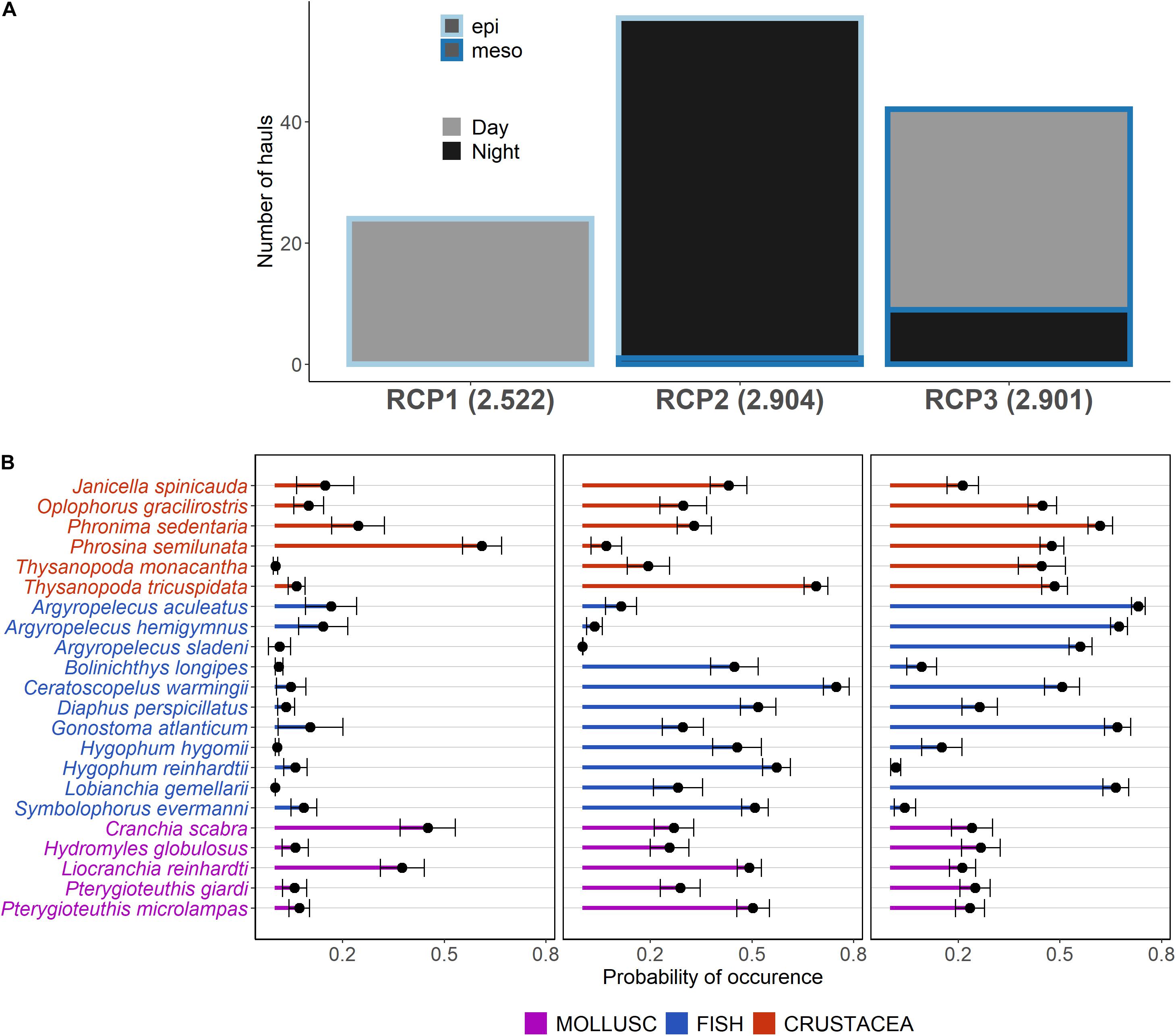
Figure 2. Results of the three RCP models showing the number of trawl hauls by region of common profile (RCP) or trawl haul groups with shared species’ composition color-filled by the moment of the day and outline colored by the vertical layer (epi: epipelagic, 10–200 m; and meso: mesopelagic, 200–600 m), Shannon index is indicated in parenthesis after RCP names (A). The species prevalence for each RCP shows the average of occurrence probability for each species. Standard deviations and means are calculated by taking 500 bootstrap samples of model parameters and generating expected probability of occurrences for each species in each RCP (B).

As the aim of the study was to explore nuanced assemblages and to determine the influence of parameters other than depth and day/night on the assemblages; the rest of the results focus on the nine-assemblage solution.

Description of the Nine Assemblages

The RCP model diagnostic plots indicate that the model was adequate to describe variation in data (i.e., independence of observed data, good residual distribution, and residuals’ independence to fitted values) (Supplementary Figure S5). There was also no evidence of residual spatial autocorrelation by species (Supplementary Figure S6).

RCP1 of the nine-assemblage model was similar to the day epipelagic assemblage of the three-assemblage model with a small number of species and the dominance of Phrosina semilunata (crustacean) and Cranchia Scabra and Liocranchia reinhardti (mollusks) (Figure 3). RCP7 also demonstrated a low Shannon index (2.11) with few species dominating the assemblage and was mainly composed by the crustacean Phronima sedentaria and Phrosina semilunata as well as the fish Argyropelecus aculeatus.

FIGURE 3

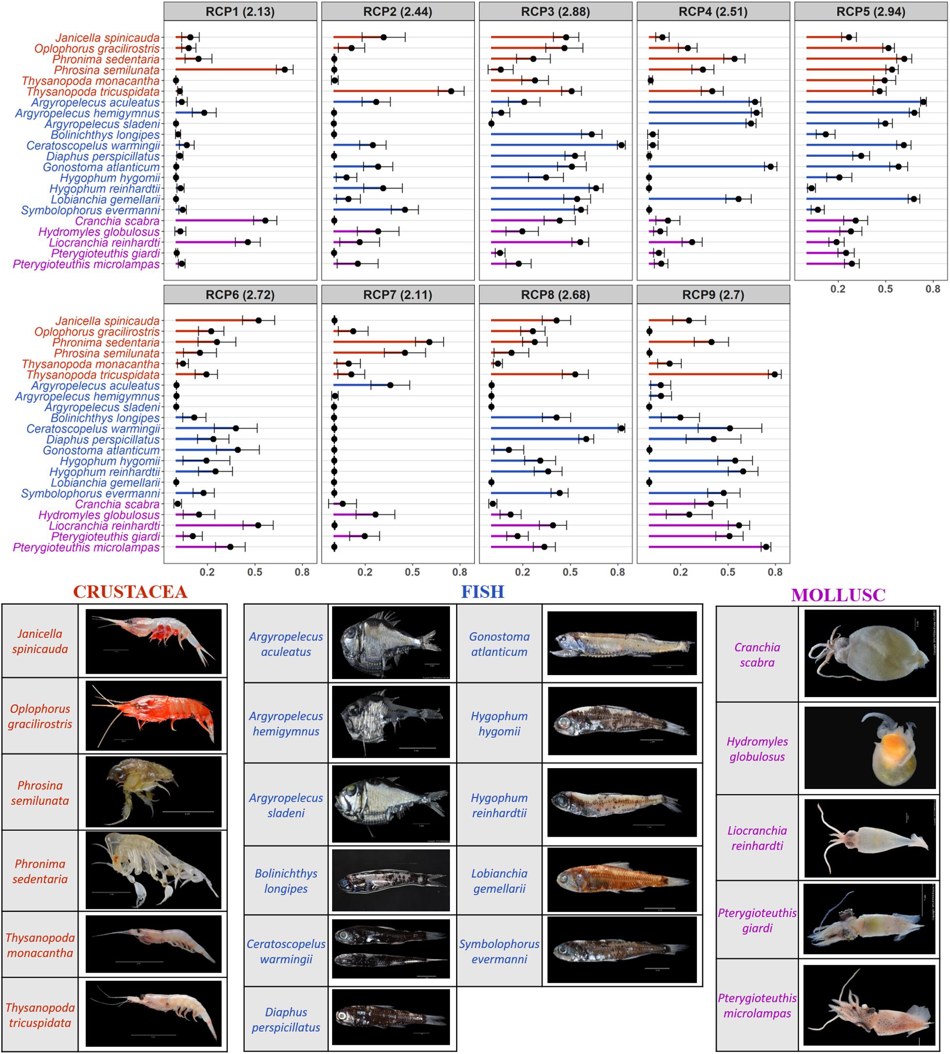
Figure 3. Results of the nine RCP models showing the species prevalence for each region of common profile (RCP) or trawl haul groups with shared species’ composition (RCP 1–9), i.e., the average and standard deviation of occurrence probability for each species. Standard deviations and means are calculated by taking 500 bootstrap samples of model parameters and generating expected probability of occurrences for each species in each RCP. Shannon index is indicated in parenthesis after RCP names. All pictures are © SPC/FEMA/Elodie Vourey.

Other assemblages were more diverse (RCP2, RCP3, RCP4, RCP5, RCP6, RCP8, and RCP9) with a Shannon index above 2.5 and an index above 2.8 for RCP3 and RCP5 (Figure 3). RCP2 was mostly dominated by Thysanopoda tricuspidata, and RCP3 was characterized by a large proportion of fish species. The high occurrence of the three Argyropelecus sp. characterized RCP4 and RCP5, and those two RCPs were correlated (Spearman correlation of 0.72; Table 2). RCP6 was similar to RCP3 (Spearman correlation of 0.66) but with a smaller proportion of all species. RCP5 was dominated by Ceratoscopelus warmingii. Finally, RCP8 and RCP9 were similar (Spearman correlation of 0.7) with Thysanopoda tricuspidata and Ceratoscopelus warmingii dominating those assemblages, and RCP9 had the largest proportion of mollusk species.

TABLE 2

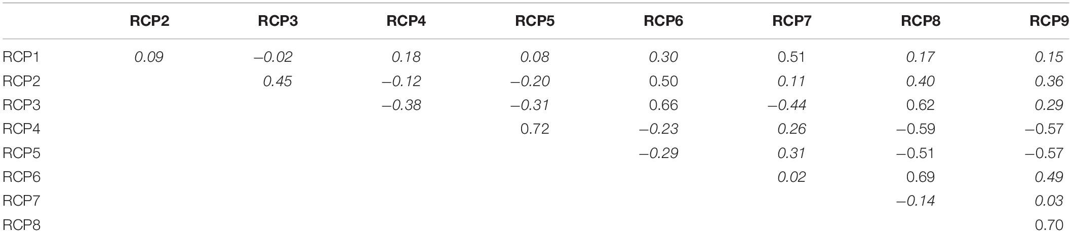
Table 2. Spearman correlation between RCPs; italic numbers are non-significant correlations.

Environmental Variables Influencing Assemblages

Probabilities of RCPs’ presence were especially driven by the depth and the moment of the day (Figures 2, 4). A succession of RCPs was observed along the depth (Figure 4A).

FIGURE 4

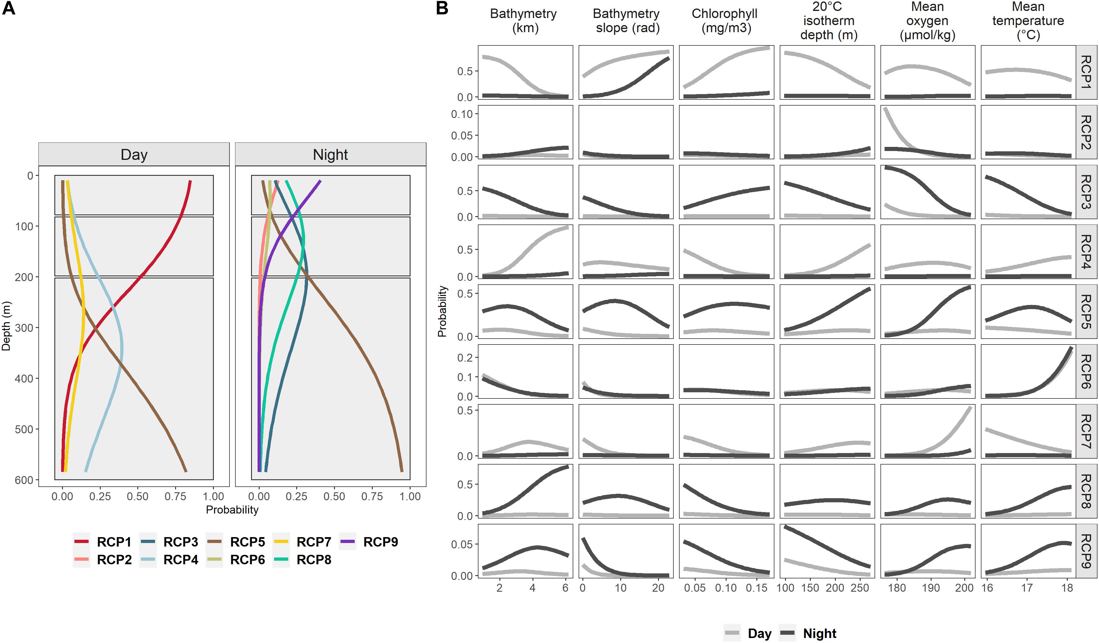
Figure 4. Probability of each of the nine RCPs according to depth during day and night periods (A), and according to bathymetry, bathymetry slope, chlorophyll-a concentration, 20°C isotherm depth, mean oxygen concentration, and mean temperature during the day (gray line) and during the night (black line) (B). (A) Black boxes show vertical layers used for predictions in Figure 5.

During the day, mainly four RCPs were observed: RCP1 prevailed in the top 200 m, RCP4 and RCP7 between 250 and 400 m, and RCP5 dominated deeper than 400 m. Among the RCPs found during the day and sharing the same vertical layer (RCP4 and RCP7), RCP4 was mostly favored by bathymetry deeper than 4000 m, and RCP7 optimal values were mostly for high mean oxygen concentration (Figure 4B).

At night, layers deeper than 200 m were mainly also occupied by RCP5, and in 80–200 m, RCP8 and RCP3 dominated. Low oxygen values and cold temperature were important for RCP3, and deep bathymetry for RCP8. RCP9, RCP2, and RCP6 were found in waters shallower than 200 m with a predominance of RCP9. RCP2 appeared only in waters with low oxygen concentration, RCP6 in warm mean temperature waters (above 17.5°C), and shallow isotherm 20°C was the factor influencing RCP9.

Spatial and Temporal Distribution of Predicted Assemblages

As explained in Section “Model predictions,” no extrapolation was done; i.e., spatial maps of RCPs occurrence were predicted based on environmental variables within the observed range of each variable (Supplementary Figure S3).

Based on night RCP depth distribution (Figure 4A), three vertical layers were selected to map out RCP probabilities on a 1/4° spatial grid. Vertical limits of these layers were determined when dominant assemblages changed (i.e., RCP9 dominated from the surface down to 80 m, then RCP3 and RCP8 for depths between 80 and 200 m and RCP5 in the deeper mesopelagic layer). We averaged predictions over these three vertical layers and by season (warm season from December to May and cold season from June to November), and spatial predictions were used to visually examine the spatial and temporal extent of species assemblages.

During the day, RCP1 dominated almost the whole EEZ between 10 and 200 m except for the extreme north (RCP2 and RCP4) and the region around Chesterfield/Bellona reef for the whole water column (RCP6) (Figure 5). RCP5 (south) and RCP4 (north) occupied the entire EEZ deeper than 200 m except for the Chesterfield/Bellona area (RCP6). Small changes were observed across seasons: RCP spatial distributions were very similar for the two seasons with only a switch from RCP2 to RCP4 in the north between 80 and 200 m, the presence of the RCP7 in the extreme south, and a small southward extension of RCP4 during the warm season.

FIGURE 5

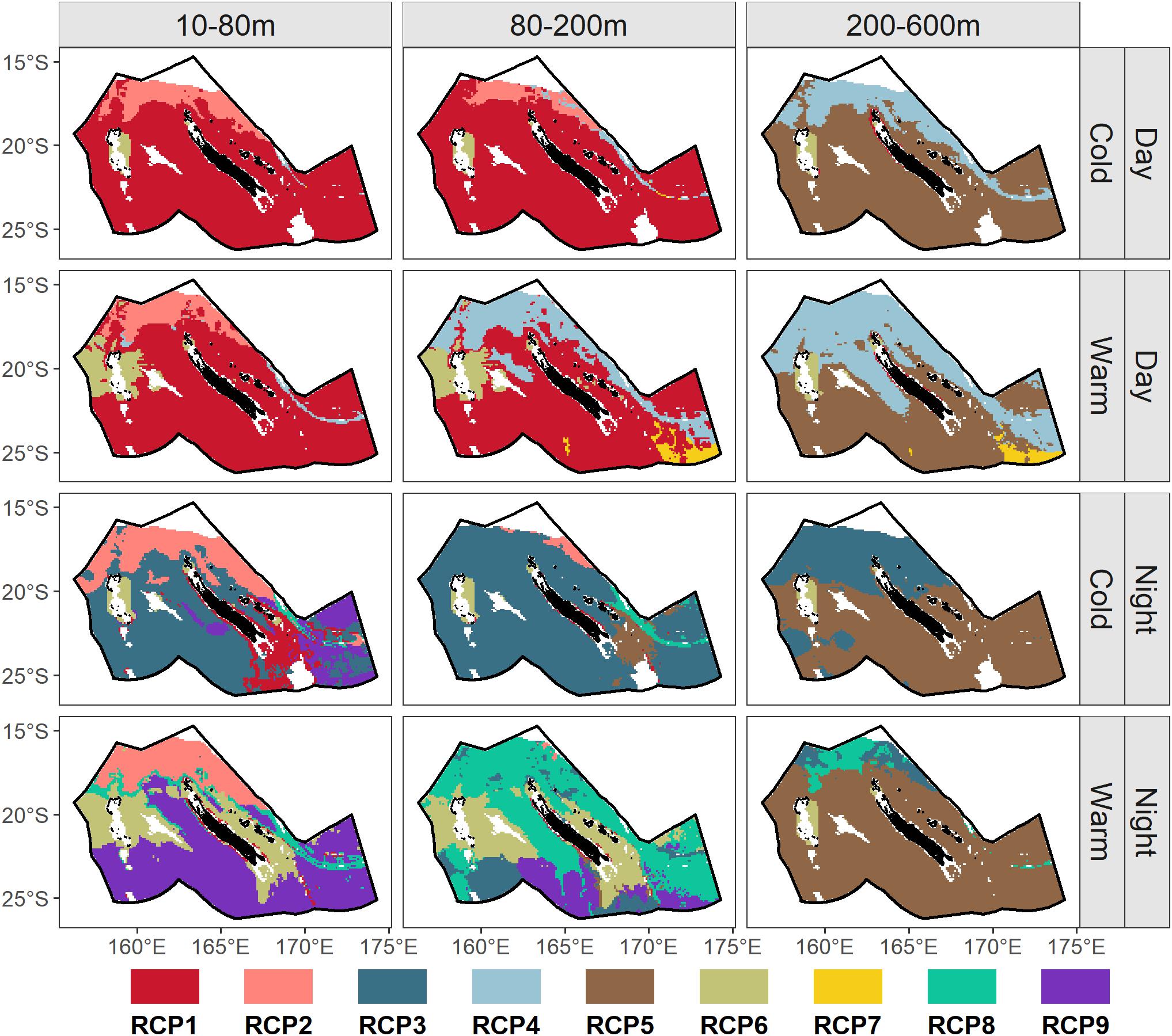
Figure 5. Most probable predicted RCP for three different vertical layers: 10–80, 80–200, and 200–600 m (columns) and for day and night periods during cold and warm seasons (rows) for the whole New Caledonian EEZ.

Night predictions were more partitioned and spatially variable; there were differences among the three vertical layers with a general north/south splitting. Over 10–80 m, RCP2 dominated the area north of 20°S during the two seasons, and RCP9 (warm season) and RCP3 (cold season) dominated the southern area. Between 80 and 200 m, RCP3 prevailed during the cold season, whereas RCP8 prevailed during the warm season. The 200–600 m spatial distribution at night was very close to that of the day with a dominance of RCP5. RCP6 was the most probable assemblage at night and day around Chesterfield/Bellona reef.

By averaging RCP Shannon indices weighted by their corresponding RCP probabilities, spatial patterns of the day–night, warm–cold seasons, and 10–600 m, mean micronektonic diversity was assessed (Figure 6). The mean spatial distribution of Shannon indices across the EEZ showed larger values in the southwest (∼2.73) compared to the northern part (∼2.64) or the southeast part (∼2.63) of the EEZ, especially around Chesterfield/Bellona reef and south of Fairway-Lansdowne Banks. The channel between the Main Island and Loyalty Islands also had a high Shannon index (∼2.74).

FIGURE 6

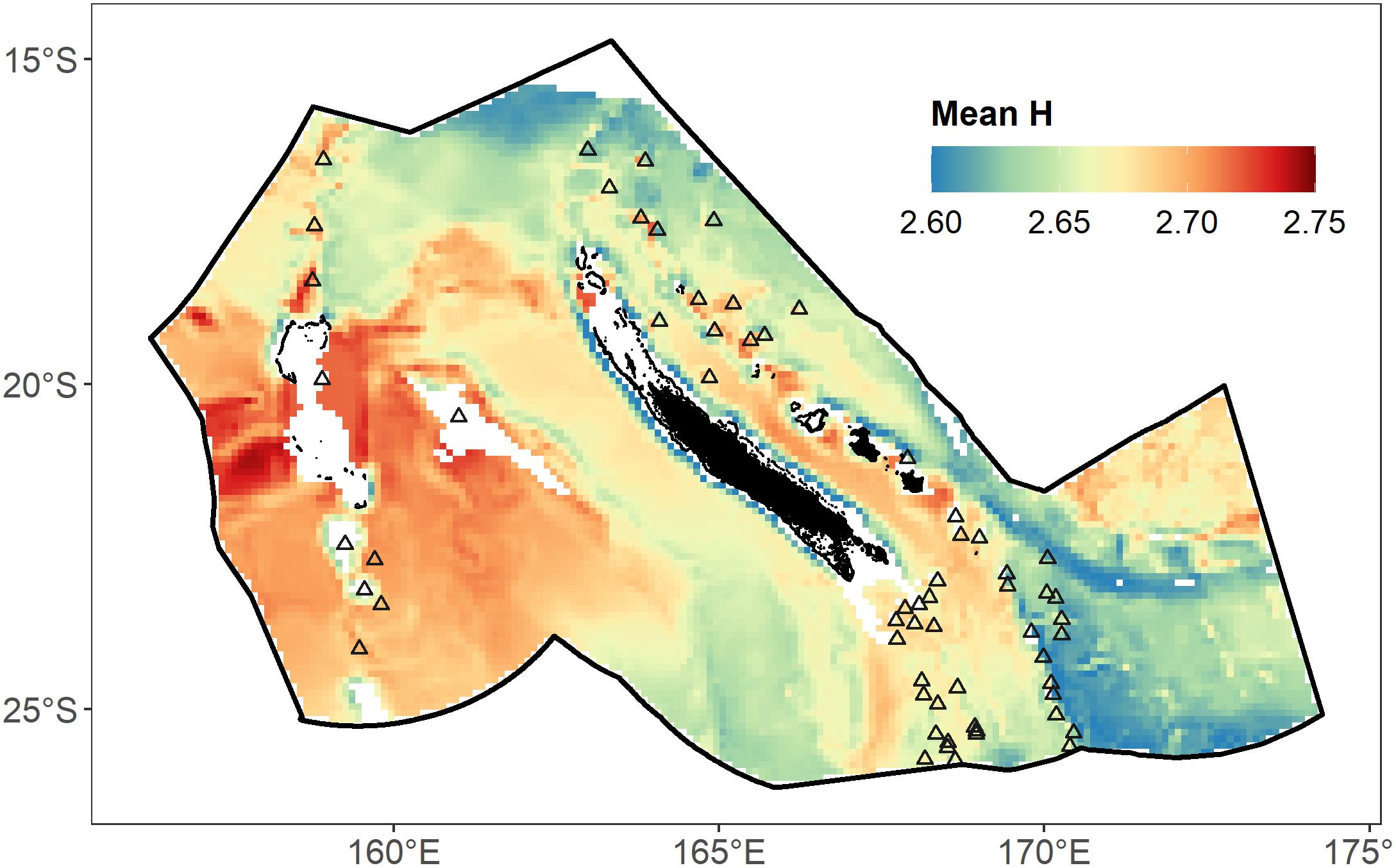
Figure 6. Proxy of Shannon index (mean H) predicted in the whole studied area on average for depths between 0 and 600 m and for day and night combined. Black triangles indicate the location of seamounts according to Allain et al. (2008).

Vertical and Spatial Distribution per Species

Based on the AUC criterion (Table 3), predictions of distribution should be considered with caution for a number of species, such as Phronima sedentaria, Liocranchia reinhardti, and Hygophum hygomii with AUC smaller than 0.7. Hydromyles globulosus had the smallest AUC (0.37) of all species.

TABLE 3

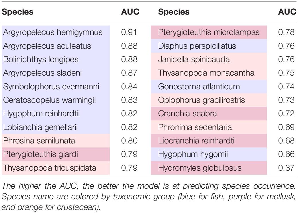
Table 3. Area under the curve (AUC) values by species.

Recall that night and day vertical profiles were used to assess diel vertical behavior: A species was identified as migrant when its night–day anomaly was larger than 0.2, as weakly migrant when the anomaly was between 0.1 and 0.2, and as resident when the anomaly was smaller than 0.1 (Table 4).

TABLE 4

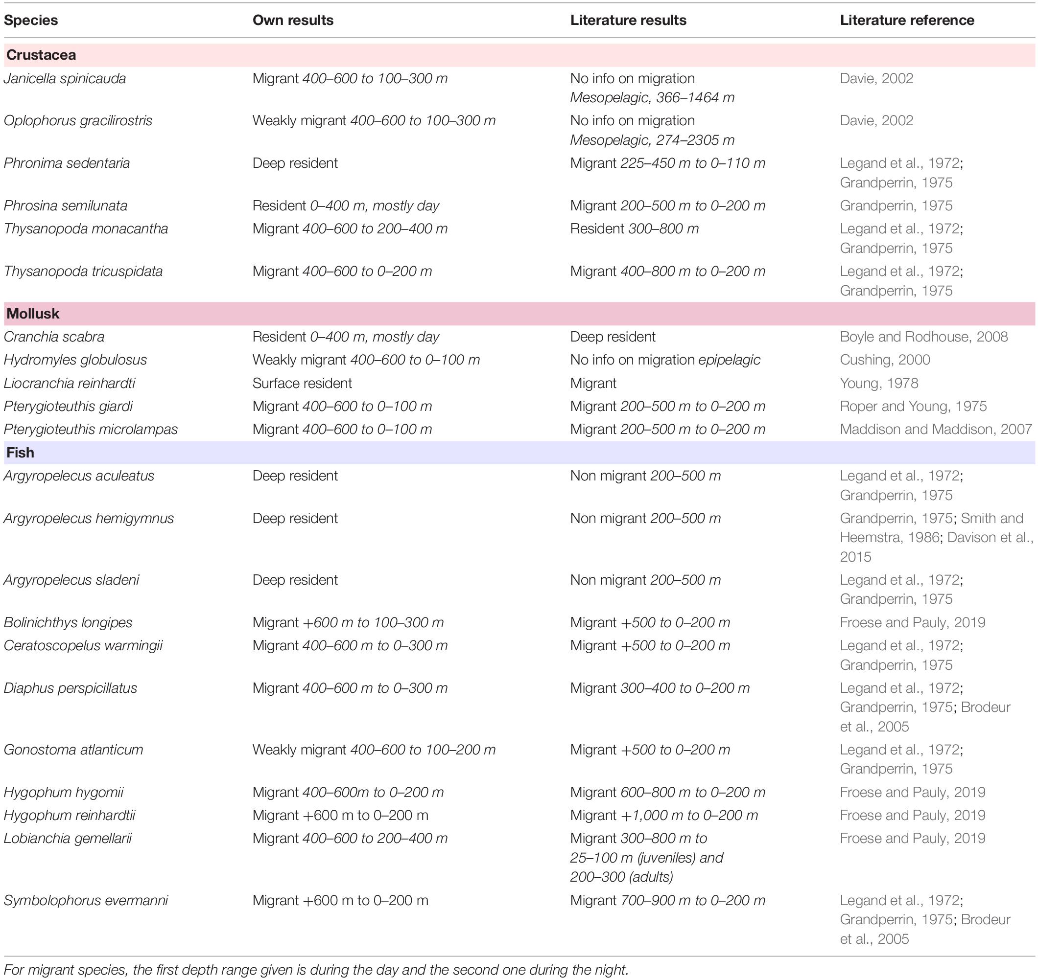
Table 4. Comparison of the species vertical behavior between our results and the literature, ordered and colored by taxonomic group.

Among fish, the three marine hatchetfish Argyropelecus species were found to be resident deeper than 200 m (Figure 7). The lanternfish (family Myctophidae), Bolinichthys longipes, Ceratoscopelus warmingii, Diaphus perspicillatus, Hygophum hygomii, Hygophum reinhardtii, Lobianchia gemellarii, and Symbolophorus evermanni were identified as migrant. B. longipes, the two Hygophum sp., and S. evermanni were predicted to stay deeper than 600 m and the others deeper than 400 m during the day. During the night, the predicted occurrence was higher in the 100–300 m layer than for the 0–100 m vertical layer for B. longipes, C. warmingii, D. perspicillatus, and L. gemellarii. Finally, Gonostoma atlanticum was identified as weakly migrant from 400 to 600 m during the day to 100–200 m during the night.

FIGURE 7

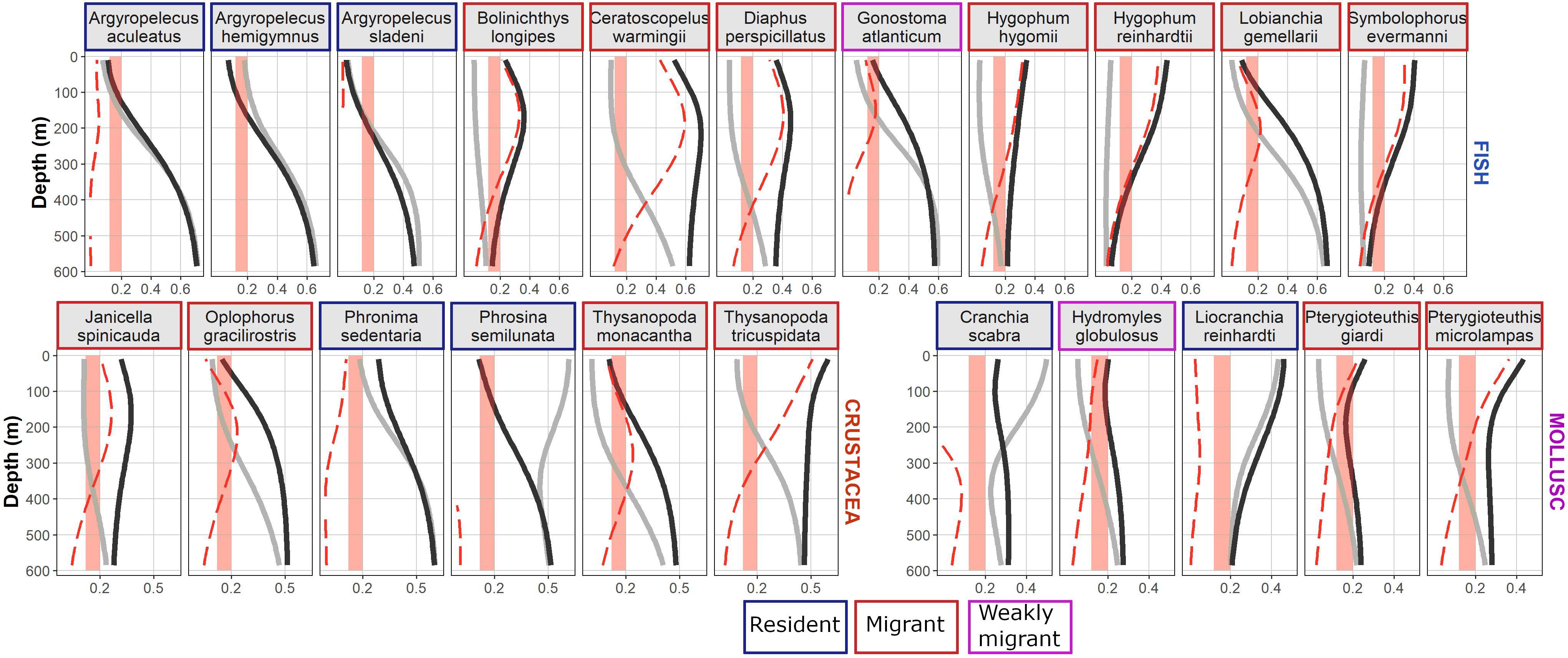
Figure 7. Species occurrence probability predicted by depth according to day (light gray line) and night (black line). Red dotted lines show positive anomaly between night and day (i.e., night probability – day probability). Vertical red stripes highlight the [0.1–0.2] probability range used to determine the species migratory behavior (resident: night–day anomaly smaller than 0.1; weakly migrant: night–day anomaly between 0.1 and 0.2; and migrant: night–day anomaly higher than 0.2). Colored outline around species name indicates the migratory behavior.

For crustaceans, Janicella spinicauda, Oplophorus gracilirostris, Thysanopoda monacantha, and Thysanopoda tricuspidata were found to have a migrant behavior, migrating from 400 to 600 m in the day to 100–300 m at night for the three first species and migrating from 400 to 600 m in the day to 0–200 m at night for T. tricuspidata. Phronima sedentaria was identified as resident in the 200–600 m vertical layer. Phrosina semilunata was identified as resident in the 10–600 m layer.

For mollusks, a weakly migrant behavior was associated to Hydromyles globulosus from 400 to 600 m in the day to 0–200 m at night and a migrant behavior to Pterygioteuthis giardi and Pterygioteuthis microlampas from 400 to 600 m in the day to 0–100 m at night. On the contrary, Liocranchia reinhardti and Cranchia scabra were classified here as epipelagic resident (i.e., 0–200 m).

Finally, the average spatial distribution over the 10–600 m depth layer and over day and night was investigated for each of the 22 species (Figure 8).

FIGURE 8

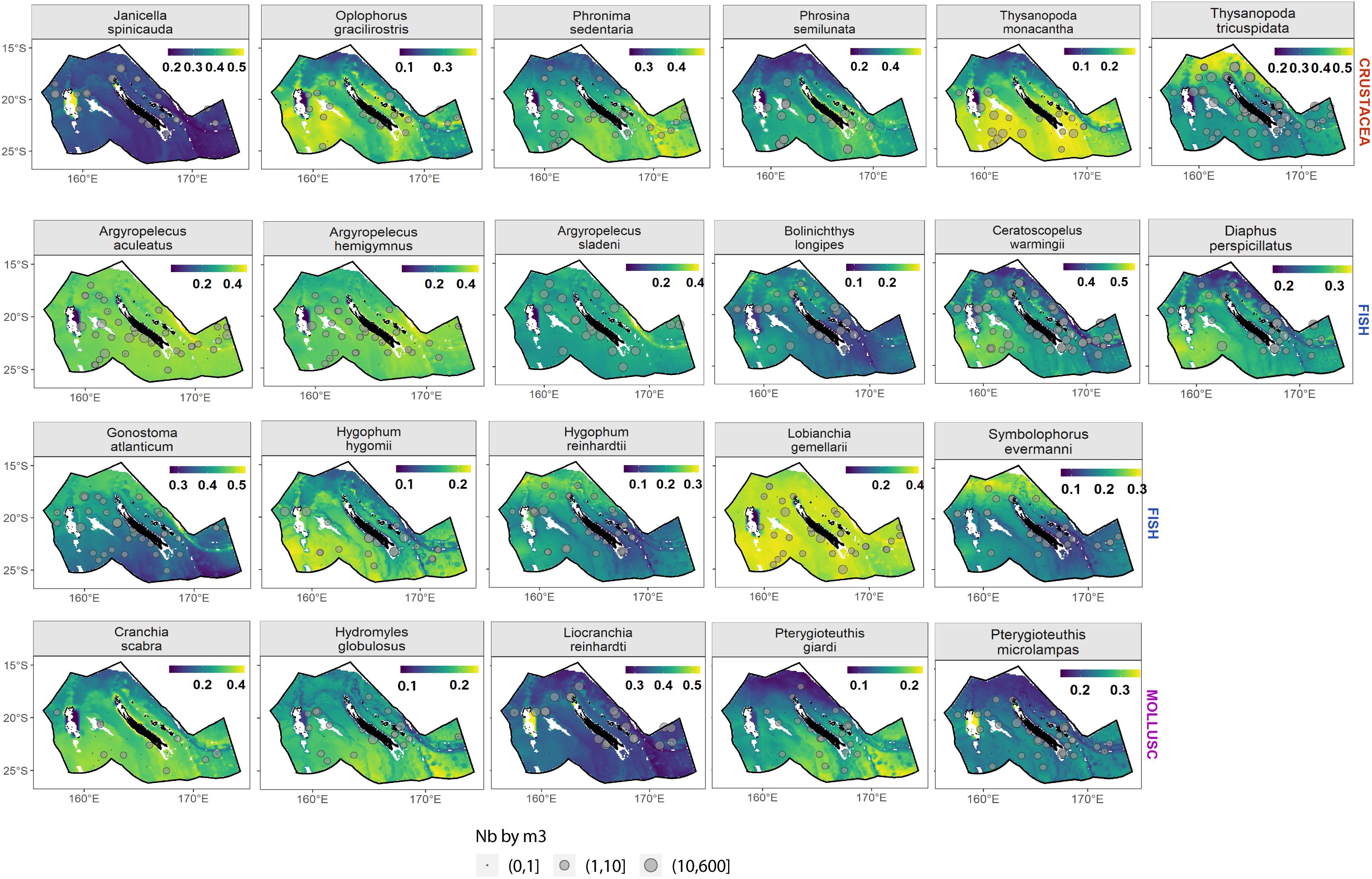
Figure 8. Spatial prediction of species occurrence probability on average between day and night and for all depth with a 10 m vertical resolution between 10 and 600 m. Gray points show raw observed data in number of specimens per m³.

Regarding crustacean species, Janicella spinicauda was predicted to be more abundant in shallow waters, especially around Chesterfield reef. On the contrary, Oplophorus gracilirostris, Phronima sedentaria, and Thysanopoda monacantha were predicted to be absent around Chesterfield reef with the three latter species more abundant south of 20°S. Phrosina semilunata was found in shallow waters close to the coast and, on average, was more abundant in the south than in the north of the EEZ. Finally, Thysanopoda tricuspidata was mainly predicted in the extreme north of the EEZ.

Regarding mollusks, Cranchia scabra and Hydromyles globulosus had higher probability of presence in the southern part of the EEZ with a homogenous repartition in the south. Pterygioteuthis giardi was also predicted to be more abundant in the south but with a less homogenous distribution and especially in deeper waters. Spatial patterns were weaker for Liocranchia reinhardti and Pterygioteuthis microlampas with larger abundance predicted around Chesterfield reef, and P. microlampas was slightly more abundant south of 20°S.

Finally, among fishes, three marine hatchetfish, Argyropelecus aculeatus, A. hemigymnus, and A. sladeni, were predicted to have the same spatial patterns with a higher abundance in regions characterized by high bathymetry slope and lower abundance around Chesterfield. Bolinichthys longipes was mainly predicted as present in the western part of the EEZ. Ceratoscopelus warmingii, Diaphus perspicillatus, and Hygophum hygomii were predicted with slightly higher probability of presence in the south of the EEZ, especially south of Chesterfield/Bellona reef and of Fairway-Lansdowne Banks. The two species of Myctophidae, Hygophum reinhardtii, Symbolophorus evermanni, and the species of Gonostomatidae, Gonostoma atlanticum, had similar spatial distribution and were found relatively homogeneously in the entire New Caledonian EEZ but with a slightly higher probability in the northern part of the EEZ. Finally, the presence of Lobianchia gemellarii was predicted as present almost everywhere.

Discussion

Community ecology (species assemblages) and ecosystem ecology (physical processes driving interactions with species) are primordial to the understanding of complex ecosystem functioning (Loreau, 2010). The present study described the structure and the diversity of the micronektonic community and the habitats of their species in the New Caledonian EEZ (southwest Pacific). A focus was made on the 22 most frequent species (out of 252 identified) to adequately model their spatial distribution. Using the RCP methodology, the data set was split into small numbers of assemblages (three and nine). The moment of the day and the sampling depth were the two parameters influencing the three-assemblages model. There were larger proportions of fish and crustaceans in day and night mesopelagic assemblages and a large proportion of mollusks in the night epipelagic assemblage. By splitting the data set into nine major assemblages, the moment of the day and the depth of sampling remained the main driving parameters; however, influence of other environmental variables was detected. Variables such as mean oxygen concentration, mean temperature, and bathymetry also influenced micronekton assemblages and induced a specific north/south pattern. Three major daytime assemblages were identified, covering the whole EEZ, and showed a depth layer structure. One assemblage dominated in waters shallower than 200 m, and the other two were found in deeper waters (down to 600 m) in the north and in the south. The four major night communities were more diverse with a patchier spatial distribution and two depth changes, at approximately 80 and 200 m. The predominant night northern assemblage (RCP2) in the top 80 m was dominated by mollusks and fish species, whereas the southern assemblage (RCP9) was dominated by crustacean and fish species. The 80–200 m nighttime assemblages were characterized by more cephalopods and fish in the north than in the south. Generally, assemblages’ spatial distribution indicated that the southwest part of the EEZ was more diverse than other regions. Finally, the spatial distribution of 22 frequent species was described as well as their vertical behavior.

Statistical Framework

To our knowledge, previous studies on micronekton mostly used clustering methods based on various dissimilarity metrics (e.g., Drazen et al., 2011; Parker et al., 2015; Eduardo et al., 2018; Flynn et al., 2018). Here, an alternative was offered to simultaneously classify trawl data in homogenous groups and study their links with environmental drivers. We confirmed Hill et al.’s (2017) conclusions about RCP capacities and extended the application domain moving from demersal fish of the Kerguelen Plateau to pelagic micronektonic communities in a subtropical region. The method was especially useful for micronekton species that had a complex vertical habitat and behavior. Indeed, the approach allowed taking into account the DVM signal by including moment of the day and trawl depth as well as looking at the influence of oceanographic parameters on more subtle variations in assemblages. Moreover, the species occurrence probabilities were predicted for all 0–600 m depths, and therefore, an incomplete or unbalanced data set composed of a small observation number (e.g., missing sample depths) could be used to assess species vertical habitat. Hence, the model was no longer limited to the depth sampled as presented by Williams and Koslow (1997) or Nishikawa et al. (2001). A complete description of vertical habitat by species could be especially useful to integrate in biogeochemical models over depth for example (Aumont et al., 2018). The largest weakness of that statistical modeling approach was the removal of the less frequent species. Indeed, to have robust statistical relationships, the number of observed occurrences had to be significant (i.e., more than 33 presences in the present study). Consequently, all conclusions were only made on 22 species although more than 250 were identified in the region. For these reasons, conclusions on diversity spatial distribution, measured here with the Shannon index, concerned only a small number of species. A different analysis including all species would be an interesting next step to describe the total micronektonic species diversity but would require the design of another statistical methodology.

There was no link between the total number of observations and the model ability to efficiently predict the probability of presence, quantified by AUC. For example, Phronima sedentaria had one of the worst AUCs, whereas it was the third most frequent species. It was assumed that species with a small AUC, such as Phronima sedentaria, had large environmental tolerance, at least for variables included in the RCP model. This large tolerance window complicated the fit of the relationships between environmental gradient and the probability of presence. Therefore, to improve predictions of spatial distribution for these species, sampling may need to be performed in more contrasted environmental conditions. The other hypothesis was that other environmental variables (e.g., the salinity) were missing in the model, and it could be more influential over those species.

Ecoregionalization of Prey Communities

It should be noted that the trawl used in this study did not allow sampling of micronekton communities in the top 10 m, resulting in the likely absence of an important community as previously shown in the southern ocean (Flores et al., 2014). Moreover, mid-water trawls are known to select some species due to net avoidance behavior by some organisms and to select some specific size ranges of organisms (Heino et al., 2011; Kaartvedt et al., 2012). This trawl selectivity could be tested by using different trawls to sample the same layers (De Robertis et al., 2017). Finally, as the trawl stays open during setting and hauling, layers sampled could be mixed with other layers during these two periods. In the absence of an open–close trawl, future specific hauls and sampling strategies are needed to answer this question. We checked, and in the literature, the vertical habitats of the 22 studied species were deeper than 0–10 m. Moreover, as the studied species in the present study were the most abundant, there were certainly mostly collected during the 30 min of hauling in comparison to the few minutes in the upper layers.

During the night, communities of the northern region were relatively stable across seasons. On the contrary, communities in the south changed in waters shallower than 200 m during the night across seasons. Those differences could be explained by environmental conditions as the assemblages predicted in the south of 20°S were supported by high oxygen values and cold temperature, whereas northern assemblages were supported by low oxygen and warm temperature.

The north–south transition observed between the communities RCP2–RCP8 and RCP3–RCP6–RCP9 at night in the surface layer around a latitude 20°S appeared to be mainly linked to a temperature meridional gradient. Spatial patterns of the temperature in the New Caledonian EEZ indeed shows a strong north–south gradient, well delimited around 20°S (Menkes et al., 2015), which also reflects different oceanographic conditions more generally (the northern part is influenced by warm waters coming from the equator, and the southern part by cold and rich waters coming from the southeast). Therefore, 0–600 m mean temperature appeared to delimit large homogeneous hydrodynamic regions constraining micronekton habitats rather than a direct biological impact. The 0–600 m averaged oxygen concentration was another important variable influencing a community’s probability of presence. The link between oxygen concentration and micronekton vertical distribution has been studied previously using acoustic estimates. For instance, in the South Pacific, the lower vertical expansion of epipelagic micronekton layers was found to be limited by the minimum oxygen depth (Bertrand et al., 2010). Bianchi et al. (2013) demonstrated on a global scale that the higher the oxygen concentration at depth, the deeper the micronekton deep layer was during the daytime. Results from the present study as well as from Suntsov and Domokos (2013) in the north Pacific show that oxygen also influenced the micronekton species composition with higher oxygen values linked to a richer community with potentially a larger proportion of mollusks.

In addition to oceanographic parameters, we observed that micronekton assemblages were influenced by bathymetry, which is very diverse in New Caledonia with ridges, seamounts, trenches, and sedimentary basins (Gardes et al., 2014). According to Escobar-Flores et al. (2018), shallower waters offer lower-quality habitat for mesopelagic organisms and may induce a densification of organisms in the upper layers of the water column. Spatial predictions of the Shannon index showed a higher diversity around seamounts in the north of the Loyalty Islands (i.e., around the Astrolabe and Petrie reefs) and north and south of Chesterfield/Bellona reef. The small overall range of Shannon values predicted (about 0.15) could be linked to the methodology used and because it was calculated only on 22 species.

Climate change will have a profound impact on ecosystem structure (Lotze et al., 2019), but impacts on the micronekton component are largely unknown (St. John et al., 2016). Based on the present study, the predicted decrease of oxygen concentration (Stramma et al., 2010, 2008) could favor RCP2 (dominated by Thysanopoda tricuspidata) and RCP3 (large proportion of fish) in the future, whereas the predicted temperature increase (Bopp et al., 2013) could favor RCP6 (Chesterfield assemblage), RCP8 (dominated by Ceratoscopelus warmingii), and RCP9 (large mollusk proportion). Moreover, changes in oxygen minimal depth would change the vertical distribution of micronektonic communities, potentially making them more vulnerable to epipelagic predators (Stramma et al., 2010; Olson et al., 2014). As predictions of future marine oceanographic conditions are becoming more and more precise and realistic, one next step could be to forecast future communities by forcing the RCP model with climate change model outputs with both present and future simulations to measure change in communities.

The strong latitudinal shift in micronekton assemblages found in our study mirrored Flynn and Marshall (2013) and Flynn et al. (2018) in bioregionalization of the eastern Australia region. Communities described in the present study were in agreement with previous studies in the Coral Sea with the dominant fish species belonging to the families Gonostomatidae, Sternoptychidae, and Myctophidae (Grandperrin, 1975; Flynn and Paxton, 2012; Sutton et al., 2017). However, the 22 most abundant species identified were completely different from the 20 most abundant species described in the southern of Tasmania even if some species were found in both studies (A. aculeatus, A. hemigymnus, C. warmingii) (Williams and Koslow, 1997). Some abundant species in this study were also found in Hawaiian waters (18°N–21°N) (e.g., B. longipes, C. warmingii, D. perspicillatus, G. atlanticum, and J. spinicauda) (Reid et al., 1991; De Forest and Drazen, 2009; Drazen et al., 2011) or close to Papua New Guinea (0°N–20°N) (e.g., B. longipes, C. scabra, D. perspicillatus, H. reinhardtii, and S. evermanni) (Duffy et al., 2017). Given those similarities and differences, an analysis on the scale of the Pacific Ocean would be a large improvement for the understanding of prey distribution.

Micronektonic Species Behavior

Vertical behaviors and spatial distribution of the 22 most frequent species were investigated in the New Caledonian EEZ. Regarding the vertical behavior, previously described vertical behavior was confirmed for 10 species (the three marine hatchetfish Argyropelecus, Ceratoscopelus warmingii, Hygophum reinhardtii, Lobianchia gemellarii, the two Pterygioteuthis species, Symbolophorus evermanni, and Thysanopoda tricuspidata); new vertical behavior was described for three species (Hydromyles globulosus, Janicella Spinicauda, and Oplophorus gracilirostris), and vertical behavior was refined for seven species (Bolinichthys longipes, Diaphus perspicillatus, Gonostoma atlanticum, Hygophum hygomii, Liocranchia reinhardti, Phronima sedentaria, and Thysanopoda monacantha) (Table 4). No clear vertical patterns were associated to C. scabra and P. semilunata. These results indicate that the RCP method appears to be a valuable technique to determine micronekton vertical behavior. Spatial predictions of the species distribution were very similar to the bathymetry pattern, highlighting the importance of this parameter in species distribution and also in assemblage composition.

Concerning C. scabra and P. semilunata, there was a larger proportion of these species in the epipelagic layer (0–200 m) during the day in comparison to the night. A sampling artifact could explain this result: The presence of a large mix of species during the night could be conducive to a less efficient sampling of those two species and their absence in the epipelagic night hauls. This sampling artifact appears more plausible based on literature results than an inversed migration (from surface at day to deep at night).

The present study participated in improving the understanding of how sensitive all micronekton species are to oceanographic variables (physical and biogeochemical), information needed to fully evaluate the impact that climate change could have on top predators’ food (Choy et al., 2016). Eleven species (A. aculeatus, A. sladeni, C. scabra, H. globulosus, L. reinhardti, O. gracilirostris, P. sedentaria, P. semilunata, P. giardi, P. microlampas, and T. tricuspidata) have been observed in predators’ stomach contents in the western and central Pacific Ocean database of the Pacific Community³ (Sanchez et al., 2018) (e.g., Coryphaena hippurus, Kajikia audax, Katsuwonus pelamis, Lampris guttatus, Sphyraena barracuda, Thunnus albacares, Thunnus obesus, Xiphias gladius). Lanternfish species (or Myctophidae) are also a non-negligible part of predators’ diets (Brodeur et al., 2005; Williams et al., 2014), and although Myctophidae are found very often in stomach contents (Elodie Vourey, personal communication), their quick digestion limited their identification at the species level and explained their absence in the previously cited species list. The 22 most frequent micronekton species found in this study were also observed in other predators’ diet studies in the Pacific Ocean (Griffiths et al., 2009; Kuhnert et al., 2012; Olson et al., 2014; Portner et al., 2017), corroborating the importance of this group in the pelagic ecosystem and reinforcing the need for a better understanding of their dynamics (St. John et al., 2016). The predicted spatial distribution by species would help to improve the predator niche modeling in future studies.

Link to Acoustics

Two previous studies analyzed the acoustic data from the same Nectalis surveys to link the mean 20–120 m acoustic echo-intensity and the 0–600 m vertical acoustic profiles to environmental conditions (Receveur et al., 2019, 2020). They proposed a bioregionalization of the New Caledonia EEZ based on the micronekton vertical distribution and identified three homogenous regions during the day: (i) north of 21°S with a weak deep scattering layer (DSL) and a weak shallow scattering layer (SSL); (ii) south of 21°S and west of 165°E (intense SSL at 80 m and very intense SSL at 30 m); and (iii) south of 21°S and east of 165°E (intense SSL and very intense DSL at 550 m). The spatial extent of assemblages found in the present study were similar to the three homogenous regions defined based on acoustic profiles. This result reinforced the useful contribution of acoustics data to characterize mesopelagic organisms’ distribution. However, gelatinous organisms are known to be responsible for a significant part of the acoustic signal (Warren, 2001; Proud et al., 2018), and the development of methods capable of including these organisms in trawl analyses is crucial to more accurately compare acoustics and haul data. Therefore, a study focusing on the direct link between trawl content and multifrequency acoustic signal is needed to fully understand these complex links and to be able to quantify a total micronekton biomass for the region. Toward that end, it would be necessary to group species that respond similarly in terms of acoustics (e.g., “fluid-like,” “with gaz”). Yet, in order to deduce biomass estimation from acoustic data, knowledge of a community’s species composition and of its target strengths is primordial. Given the high species diversity found in our study, going further into transforming acoustic signal into biomass appears very challenging in the region (Fielding, 2004; Godø et al., 2009).

Natural Park of the Coral Sea Management

The creation of the Natural Park of the Coral Sea is recent (2014), and the management plan is still under development. The first management measures focused primarily on isolated reefs and islands and not on the oceanic areas.⁴ Recently, part of Chesterfield, Bellona, Entrecasteaux, Petrie, and Astrolabe (see Figure 1 for location of those features) have been classified as strict nature reserves (category I of “no human activities authorized” according to IUCN protected area classification or “1-No take-No go” according to the classification of Horta e Costa et al., 2016), including waters with a bathymetry shallower than 1000 m (Supplementary Figure S7). Based on results from this study, the Petrie and Astrolabe reefs seem to aggregate a high number of mesopelagic organisms’ compared to the surrounding area. Hence, these areas appear to be good candidates to implement a higher degree of protection level on offshore areas as well. The southwestern part of the EEZ (south of 22°S and west of 164°E) could be another area of interest for management as the micronekton assemblage (RCP3) was composed of a large number of species identified as prey for top predator species important for the pelagic ecosystem.

Conclusion

By analyzing the abundance of the 22 most frequent species collected in 123 pelagic trawls and with the help of an innovative multivariate statistical approach, variability in micronektonic assemblages around New Caledonia in the Coral Sea was measured and linked to oceanographic drivers. The largest variability highlighted was function of depth due to DVM. Moreover, the method helped to identify areas that may be regarded as conservation areas of interest. The used could also valuably contribute to assess the climate change impact on micronektonic assemblages and distribution, a crucial knowledge with consequences for the whole pelagic ecosystem.

Data Availability Statement

The datasets generated for this study are available on request to the corresponding author.

Ethics Statement

Ethical review and approval was not required for the animal study because we had the necessary authorizations to take these samples. In addition, our sampling protocol followed that widely used in other trawling studies to collect on micronektonic specimens.

Author Contributions

AR performed the statistical analysis. AR, VA, and EV analyzed the data and interpreted the results with the help of CM, AL-D, and FM. AR, VA, and CM wrote the manuscript with the help of EV, AL-D, and FM. All the authors contributed to and provided feedback on various drafts of the manuscript.

Funding

This work has been conducted with the financial assistance of the BEST2.0 program of the European Union. The content of this document is the sole responsibility of AR and can under no circumstance be regarded as reflecting the position of European Union. This work also benefited from the financial support of the French Biodiversity Agency (OFB, Office Français de la Biodiversité).

Conflict of Interest

The authors declare that the research was conducted in the absence of any commercial or financial relationships that could be construed as a potential conflict of interest.

Acknowledgments

We thank R/V ALIS officers and crews and science parties who participated to the cruises for which data are included in the present manuscript. We also thank SPC staff and external taxonomic experts who contributed to the identification of the micronekton species.

Supplementary Material

The Supplementary Material for this article can be found online at: https://www.frontiersin.org/articles/10.3389/fmars.2020.00449/full#supplementary-material

Footnotes

1. ^ doi: 10.18142/243
2. ^ https://www.zoneco.nc/
3. ^ SPC – http://www.spc.int/ofp/PacificSpecimenBank.
4. ^ https://mer-de-corail.gouv.nc/en

References

Allain, V., Fernandez, E., Hoyle, S. D., Caillot, S., Jurado-Molina, J., Andréfouët, S., et al. (2012). Interaction between coastal and oceanic ecosystems of the Western and Central Pacific Ocean through predator-prey relationship studies. PLoS One 7:e36701. doi: 10.1371/journal.pone.0036701

PubMed Abstract | CrossRef Full Text | Google Scholar

Allain, V., Kerandel, J.-A., Andréfouët, S., Magron, F., Clark, M., Kirby, D. S., et al. (2008). Enhanced seamount location database for the Western and Central Pacific Ocean: screening and cross-checking of 20 existing datasets. Deep Sea Res. Part I 55, 1035–1047. doi: 10.1016/j.dsr.2008.04.004

CrossRef Full Text | Google Scholar

Ariza, A., Garijo, J. C., Landeira, J. M., Bordes, F., and Hernández-León, S. (2015). Migrant biomass and respiratory carbon flux by zooplankton and micronekton in the subtropical Northeast Atlantic Ocean (Canary Islands). Prog. Oceanogr. 134, 330–342. doi: 10.1016/j.pocean.2015.03.003

CrossRef Full Text | Google Scholar

Ariza, A., Landeira, J. M., Escánez, A., Wienerroither, R., Aguilar, de Soto, N., et al. (2016). Vertical distribution, composition and migratory patterns of acoustic scattering layers in the Canary Islands. J. Mar. Syst. 157, 82–91. doi: 10.1016/j.jmarsys.2016.01.004

CrossRef Full Text | Google Scholar

Aumont, O., Maury, O., Lefort, S., and Bopp, L. (2018). Evaluating the potential impacts of the diurnal vertical migration by marine organisms on marine biogeochemistry. Glob. Biogeochem. Cycles 32, 1622–1643. doi: 10.1029/2018GB005886

CrossRef Full Text | Google Scholar

Bakker, J., Wangensteen, O. S., Chapman, D. D., Boussarie, G., Buddo, D., Guttridge, T. L., et al. (2017). Environmental DNA reveals tropical shark diversity in contrasting levels of anthropogenic impact. Sci. Rep. 7:16886. doi: 10.1038/s41598-017-17150-2

PubMed Abstract | CrossRef Full Text | Google Scholar

Beaumont, N. J., Austen, M. C., Atkins, J. P., Burdon, D., Degraer, S., Dentinho, T. P., et al. (2007). Identification, definition and quantification of goods and services provided by marine biodiversity: implications for the ecosystem approach. Mar. Pollut. Bull. 54, 253–265. doi: 10.1016/j.marpolbul.2006.12.003

PubMed Abstract | CrossRef Full Text | Google Scholar

Bertrand, A., Ballón, M., and Chaigneau, A. (2010). Acoustic observation of living organisms reveals the upper limit of the oxygen minimum zone. PLoS One 5:e10330. doi: 10.1371/journal.pone.0010330

PubMed Abstract | CrossRef Full Text | Google Scholar

Bertrand, A., Bard, F.-X., and Josse, E. (2002). Tuna food habits related to the micronekton distribution in French Polynesia. Mar. Biol. 140, 1023–1037. doi: 10.1007/s00227-001-0776-3

CrossRef Full Text | Google Scholar

Bianchi, D., Galbraith, E. D., Carozza, D. A., Mislan, K. A. S., and Stock, C. A. (2013). Intensification of open-ocean oxygen depletion by vertically migrating animals. Nat. Geosci. 6, 545–548. doi: 10.1038/ngeo1837

CrossRef Full Text | Google Scholar

Bianchi, D., and Mislan, K. A. S. (2016). Global patterns of diel vertical migration times and velocities from acoustic data: global patterns of diel vertical migration. Limnol. Oceanogr. 61, 353–364. doi: 10.1002/lno.10219

CrossRef Full Text | Google Scholar

Blanc, Ph., and Wald, L. (2012). The SG2 algorithm for a fast and accurate computation of the position of the sun for multi-decadal time period. Solar Energy 86, 3072–3083. doi: 10.1016/j.solener.2012.07.018

CrossRef Full Text | Google Scholar

Bopp, L., Resplandy, L., Orr, J. C., Doney, S. C., Dunne, J. P., Gehlen, M., et al. (2013). Multiple stressors of ocean ecosystems in the 21st Century: projections with CMIP5 models. Biogeosciences 10, 6225–6245. doi: 10.5194/bg-10-6225-2013

CrossRef Full Text | Google Scholar

Borsa, P., Congdon, B., and Weimerskirch, H. (2015). Mouvements En Mer Des Puffins Fouquets de La Colonie de Temrock (Nouvelle-Calédonie): Compte Rendu de Mission, 28 Novembre–08 Décembre 2014. Marseille: IRD.

Google Scholar

Borsa, P., Corbeau, A., Mcduie, F., Renaudet, L., and Weimerskirch, H. (2014). Mouvements En Mer Des Puffins Fouquets Reproducteurs de La Colonie de Gouaro Deva (Nouvelle-Calédonie): Compte Rendu de Mission, 25 Février–14 Mars 2014. Noumea: IRD.

Google Scholar

Boussarie, G., Bakker, J., Wangensteen, O. S., Mariani, S., Bonnin, L., Juhel, J. B., et al. (2018). Environmental DNA illuminates the dark diversity of sharks. Sci. Adv. 4:eaa9661. doi: 10.1126/sciadv.aap9661

PubMed Abstract | CrossRef Full Text | Google Scholar

Boyle, P., and Rodhouse, P. (2008). Cephalopods: Ecology and Fisheries, 1st Edn. Hoboken, NJ: Wiley-Blackwell.

Google Scholar

Brodeur, R., Yamamura, O., Dower, J., Mackas, D., Iguchi, N., Kawaguchi, K., et al. (2005). Micronekton of the North Pacific. Abertillery: Eastern Shires Purchasing Organistation.

Google Scholar

Browne, M. W., and Cudeck, R. (1989). Single sample cross-validation indices for covariance structures. Multivar. Behav. Res. 24, 445–455. doi: 10.1207/s15327906mbr2404_4

CrossRef Full Text | Google Scholar

Cardinale, B., Duffy, J., Gonzalez, A., Hooper, D. U., Perrings, C., Venail, P., et al. (2012). Biodiversity loss and its impact on humanity. Nature 486, 59–67. doi: 10.1038/nature11148

PubMed Abstract | CrossRef Full Text | Google Scholar

Ceccarelli, D. M., McKinnon, A. D., Andréfouët, S., Allain, V., Young, J., Gledhill, D. C., et al. (2013). The coral sea: physical environment, ecosystem status and biodiversity assets. Adv. Mar. Biol. 66, 213–290. doi: 10.1016/B978-0-12-408096-6.00004-3

PubMed Abstract | CrossRef Full Text | Google Scholar

Cheung, W. W. L., Lam, V. W. Y., Sarmiento, J. L., Kearney, K., Watson, R., and Pauly, D. (2009). Projecting global marine biodiversity impacts under climate change scenarios. Fish Fish. 10, 235–251. doi: 10.1111/j.1467-2979.2008.00315.x

CrossRef Full Text | Google Scholar

Choy, C. A., Wabnitz, C. C. C., Weijerman, M., Woodworth-Jefcoats, P. A., and Polovina, J. J. (2016). Finding the way to the top: how the composition of oceanic mid-trophic micronekton groups determines apex predator biomass in the Central North Pacific. Mar. Ecol. Prog. Ser. 549, 9–25. doi: 10.3354/meps11680

CrossRef Full Text | Google Scholar

Christie, P., Bennett, N., Gray, N. J., Wilhelm, T., Lewis, N., Parks, J., et al. (2017). Why people matter in ocean governance_ incorporating human dimensions into large-scale marine protected areas. Mar. Policy 84, 273–284. doi: 10.1016/j.marpol.2017.08.002

CrossRef Full Text | Google Scholar

Cushing, D. H. (2000). South atlantic zooplankton, Boltovskoy, D. (Ed.) (1999) Backhuys, Leiden. J. Plankt. Res. 22, 997–997. doi: 10.1093/plankt/22.5.997

PubMed Abstract | CrossRef Full Text | Google Scholar

Davidson, L. N. K., and Dulvy, N. K. (2017). Global marine protected areas to prevent extinctions. Nat. Ecol. Evol. 1:0040. doi: 10.1038/s41559-016-0040

PubMed Abstract | CrossRef Full Text | Google Scholar

Davie, P. J. F. (2002). “Crustacea: Malacostraca: Phyllocarida, Hoplocarida, Eucarida (Part1),” in Zoological Catalogue of Australia, eds A. Wells and W. W. K. Houston (Collingwood: Csiro Publishing).

Google Scholar

Davies, T. K., Martin, S., Mees, C., Chassot, E., and Kaplan, D. M. (2012). A Review of the Conservation Benefits of Marine Protected Areas for Pelagic Species Associated with Fisheries. ISSF Technical Report. McLean, VA: International Seafood Sustainability Foundation.

Google Scholar

Davison, P., Lara-Lopez, A., and Anthony Koslow, J. (2015). Mesopelagic fish biomass in the Southern California current ecosystem. Deep Sea Res. Part II 112, 129–142. doi: 10.1016/j.dsr2.2014.10.007

CrossRef Full Text | Google Scholar

De Forest, L., and Drazen, J. (2009). The influence of a hawaiian seamount on mesopelagic micronekton. Deep Sea Res. Part I 56, 232–250. doi: 10.1016/j.dsr.2008.09.007

CrossRef Full Text | Google Scholar

De Robertis, A., Taylor, K., Williams, K., and Wilson, C. D. (2017). Species and size selectivity of two midwater trawls used in an acoustic survey of the Alaska Arctic. Deep Sea Res. Part II 135, 40–50. doi: 10.1016/j.dsr2.2015.11.014

CrossRef Full Text | Google Scholar

Diaz, S., Settele, J., and Brondizio, E. (2019). Summary for Policymakers of the Global Assessment Report on Biodiversity and Ecosystem Services of the Intergovernmental Science-Policy Platform on Biodiversity and Ecosystem Services. IPBES/7/10/Add.1. Paris: Intergovernmental Science-Policy Platform on Biodiversity and Ecosystem Services (IPBES).

Google Scholar

Dormann, C. F., Elith, J., Bacher, S., Carré, G. C. G., García Márquez, J. R., Gruber, B., et al. (2013). Collinearity: a review of methods to deal with it and a simulation study evaluating their performance. Ecography 36, 27–46. doi: 10.1111/j.1600-0587.2012.07348.x

CrossRef Full Text | Google Scholar

Dornelas, M., Gotelli, N. J., McGill, B., Shimadzu, H., Moyes, F., Sievers, C., et al. (2014). Assemblage time series reveal biodiversity change but not systematic loss. Science 344, 296–299. doi: 10.1126/science.1248484

PubMed Abstract | CrossRef Full Text | Google Scholar

Drazen, J. C., De Forest, L. G., and Domokos, R. (2011). Micronekton abundance and biomass in hawaiian waters as influenced by seamounts, eddies, and the moon. Deep Sea Res. Part I 58, 557–566. doi: 10.1016/j.dsr.2011.03.002

CrossRef Full Text | Google Scholar

Drazen, J. C., and Sutton, T. T. (2017). Dining in the deep: the feeding ecology of deep-sea fishes. Annu. Rev. Mar. Sci. 9, 337–366. doi: 10.1146/annurev-marine-010816-060543

PubMed Abstract | CrossRef Full Text | Google Scholar

Duffy, L. M., Kuhnert, P. M., Pethybridge, H. R., Young, J. W., Olson, R. J., Logan, J. M., et al. (2017). Global trophic ecology of yellowfin, bigeye, and albacore tunas: understanding predation on micronekton communities at ocean-basin scales. Deep Sea Res. Part II 140, 55–73. doi: 10.1016/j.dsr2.2017.03.003

CrossRef Full Text | Google Scholar

Eduardo, L. N., Frédou, T., Souza Lira, A., Padovani Ferreira, B., Bertrand, A., Ménard, F., et al. (2018). Identifying key habitat and spatial patterns of fish biodiversity in the tropical Brazilian continental shelf. Contin. Shelf Res. 166, 108–118. doi: 10.1016/j.csr.2018.07.002

CrossRef Full Text | Google Scholar

Ehler, C., and Douvere, F. (2009). Marine Spatial Planning: A Step-by-Step Approach Toward Ecosystem-Based Management. Paris: Unesco.

Google Scholar

Escobar-Flores, P. C., O’Driscoll, R. L., and Montgomery, J. C. (2018). Predicting distribution and relative abundance of mid-trophic level organisms using oceanographic parameters and acoustic backscatter. Mar. Ecol. Prog. Ser. 592, 37–56. doi: 10.3354/meps12519

CrossRef Full Text | Google Scholar

Fielding, S. (2004). The biological validation of ADCP acoustic backscatter through direct comparison with net samples and model predictions based on acoustic-scattering models. ICES J. Mar. Sci. 61, 184–200. doi: 10.1016/j.icesjms.2003.10.011

CrossRef Full Text | Google Scholar

Fisher, R., Knowlton, N., Brainard, R. E., and Caley, M. J. (2011). Differences among major taxa in the extent of ecological knowledge across four major ecosystems. PLoS One 6:e26556. doi: 10.1371/journal.pone.0026556

PubMed Abstract | CrossRef Full Text | Google Scholar

Flores, H., Hunt, B. P. V., Kruse, S., Volker Siegel, E. A. P., van Franeker, J. A., Strass, V., et al. (2014). Seasonal changes in the vertical distribution and community structure of antarctic macrozooplankton and micronekton. Deep Sea Res. Part I 84, 127–141. doi: 10.1016/j.dsr.2013.11.001

CrossRef Full Text | Google Scholar

Flynn, A. J., Kloser, R. J., and Sutton, C. (2018). Micronekton assemblages and bioregional setting of the great Australian bight: a temperate northern boundary current system. Deep Sea Res. Part II 15, 58–77. doi: 10.1016/j.dsr2.2018.08.006

CrossRef Full Text | Google Scholar

Flynn, A. J., and Marshall, N. J. (2013). Lanternfish (Myctophidae) zoogeography off eastern australia: a comparison with physicochemical biogeography. PLoS One 8:e80950. doi: 10.1371/journal.pone.0080950

PubMed Abstract | CrossRef Full Text | Google Scholar

Flynn, A. J., and Paxton, J. R. (2012). Spawning aggregation of the Lanternfish Diaphus Danae (Family Myctophidae) in the North-Western Coral Sea and Associations with Tuna Aggregations. Mar. Freshw. Res. 63, 1255–1271. doi: 10.1071/MF12185

CrossRef Full Text | Google Scholar

Foster, S. D., Givens, G. H., Dornan, G. J., Dunstan, P. K., and Darnell, R. (2013). Modelling biological regions from multi-species and environmental data. Environmetrics 24, 489–499. doi: 10.1002/env.2245

CrossRef Full Text | Google Scholar

Foster, S. D., Hill, N. A., and Lyons, M. (2017). Ecological grouping of survey sites when sampling artefacts are present. J. R. Stat. Soc. Ser. C 66, 1031–1047. doi: 10.1111/rssc.12211

CrossRef Full Text | Google Scholar

Friedman, J. H. (2001). Greedy function approximation: a gradient boosting machine. Ann. Stat. 29, 1189–1232.

Google Scholar

Froese, R., and Pauly, D. (2019). FishBase. Available online at: www.fishbase.org (accessed August 10, 2019).

Google Scholar

Garcia Molinos, J., Halpern, B. S., Schoeman, D. S., Brown, C. J., Kiessling, W., Moore, P. J., et al. (2016). Climate velocity and the future global redistribution of marine biodiversity. Nat. Clim. Change 6, 83–88. doi: 10.1038/nclimate2769

CrossRef Full Text | Google Scholar

Gardes, L., Tessier, E., Allain, V., Alloncle, N., Baudat-Franceschi, J., Butaud, J.-F., et al. (2014). Analyse Stratégique de l’Espace Maritime de La Nouvelle-Calédonie - Vers Une Gestion Intégrée. Brest: Agence des aires marines protégées.

Google Scholar

Garrigue, C., Clapham, P. J., Geyer, Y., Kennedy, A. S., and Zerbini, A. N. (2015). Satellite tracking reveals novel migratory patterns and the importance of seamounts for endangered south pacific humpback whales. R. Soc. Open Sci. 2:150489. doi: 10.1098/rsos.150489

PubMed Abstract | CrossRef Full Text | Google Scholar

Glover, A. G., Wiklund, H., Chen, C., and Dahlgren, T. G. (2018). Managing a sustainable deep-sea ‘Blue Economy’ requires knowledge of what actually lives there. eLife 7:e41319. doi: 10.7554/eLife.41319

PubMed Abstract | CrossRef Full Text | Google Scholar

Godø, O. R., Patel, R., and Pedersen, G. (2009). Diel Migration and Swimbladder resonance of small fish: some implications for analyses of multifrequency echo data. ICES J. Mar. Sci. 66, 1143–1148. doi: 10.1093/icesjms/fsp098

CrossRef Full Text | Google Scholar

Gotelli, N. J., and Ellison, A. M. (2012). A Primer of Ecological Statistics, 2nd Edn. Oxford: Oxford University Press.

Google Scholar

Grandperrin, R. (1975). Structures Trophiques Aboutissant Aux Thons de Longue Ligne Dans le Pacifique Sud-ouest Tropical. Ph D. Marseille: Aix Marseille Universite.

Google Scholar

Grandperrin, R., Auzende, J. M., Lafoy, Y., Lafoy, Y., Richer, de Forges, B., et al. (1999). “Swath-Mapping and related deep-sea trawling in the southeastern part of the economic zone of New Caledonia,” in Proceeding of the 5th Indo-Pacific Fish conference, (Noumea), 459–468.

Google Scholar

Griffiths, S. P., Kuhnert, P. M., Fry, G. F., and Manson, F. J. (2009). Temporal and size-related variation in the diet, consumption rate, and daily ration of Mackerel Tuna (Euthynnus Affinis) in Neritic Waters of Eastern Australia. ICES J. Mar. Sci. 66, 720–733. doi: 10.1093/icesjms/fsp065

CrossRef Full Text | Google Scholar

Guinehut, S., Dhomps, A.-L., Larnicol, G., and Le Traon, P.-Y. (2012). High resolution 3-D temperature and salinity fields derived from in situ and satellite observations. Ocean Sci. Discuss. 9, 1313–1347. doi: 10.5194/osd-9-1313-2012

CrossRef Full Text | Google Scholar

Hannah, L., Ikegami, M., Hole, D. G., Seo, C., Butchart, S. H., Peterson, A. T., et al. (2013). Global climate change adaptation priorities for biodiversity and food security. PLoS One 8:e72590. doi: 10.1371/journal.pone.0072590

PubMed Abstract | CrossRef Full Text | Google Scholar

Heino, M., Porteiro, F. M., Sutton, T. T., Falkenhaug, T., Godø, O. R., and Piatkowski, U. (2011). Catchability of Pelagic Trawls for sampling deep-living nekton in the mid-north atlantic. ICES J. Mar. Sci. 68, 377–389. doi: 10.1093/icesjms/fsq089

CrossRef Full Text | Google Scholar

Hidaka, K., Kawaguchi, K., Murakami, M., and Takahashi, M. (2001). Downward transport of organic carbon by diel migratory micronekton in the western equatorial Paci”c: its quantitative and qualitative importance. Deep Sea Res. I 48, 1923–1939. doi: 10.1016/s0967-0637(01)00003-6

CrossRef Full Text | Google Scholar

Hidalgo, M., and Browman, H. I. (2019). Developing the knowledge base needed to sustainably manage mesopelagic resources. ICES J. Mar. Sci. 76, 609–615. doi: 10.1093/icesjms/fsz067

CrossRef Full Text | Google Scholar

Hill, N. A., Foster, S. D., Duhamel, G., Welsford, D., Koubbi, P., and Johnson, C. R. (2017). Model-Based mapping of assemblages for ecology and conservation management: a case study of Demersal Fish on the Kerguelen Plateau. Diver. Distrib. 23, 1216–1230. doi: 10.1111/ddi.12613

CrossRef Full Text | Google Scholar

Hillebrand, H., Brey, T., Gutt, J., Hagen, W., Metfies, K., Meyer, B., et al. (2018). “Climate change: warming impacts on marine biodiversity,” in Handbook on Marine Environment Protection: Science, Impacts and Sustainable Management, eds M. Salomon and T. Markus (Cham: Springer International Publishing), 353–373. doi: 10.1007/978-3-319-60156-4_18

CrossRef Full Text | Google Scholar

Horta e Costa, B., Claudet, J., Franco, G., Erzini, K., Caro, A., and Gonçalves, E. J. (2016). Mar. Policy 72, 192–198. doi: 10.1016/j.marpol.2016.06.021

CrossRef Full Text | Google Scholar

Hudson, J. M., Steinberg, D., Sutton, T. T., Graves, J. E., and Latour, R. J. (2014). Myctophid feeding ecology and carbon transport along the Northern Mid-Atlantic Ridge. Deep Sea Research Part I 93, 104–116. doi: 10.1016/j.dsr.2014.07.002

CrossRef Full Text | Google Scholar

Hui, F. K. C., Taskinen, S., Pledger, S., Foster, S. D., and Warton, D. I. (2015). Model-based approaches to unconstrained ordination. Methods Ecol. Evol. 6, 399–411. doi: 10.1111/2041-210X.12236

CrossRef Full Text | Google Scholar

Kaartvedt, S., Staby, A., and Aksnes, D. L. (2012). Efficient Trawl avoidance by mesopelagic fishes causes large underestimation of their biomass. Mar. Ecol. Prog. Ser. 456, 1–6. doi: 10.3354/meps09785

CrossRef Full Text | Google Scholar

Klevjer, T. A., Irigoien, X., Røstad, A., Fraile-Nuez, E., Benítez-Barrios, V. M., and Kaartvedt, S. (2016). Large scale patterns in vertical distribution and behaviour of mesopelagic scattering layers. Sci. Rep. 6:19873. doi: 10.1038/srep19873

PubMed Abstract | CrossRef Full Text | Google Scholar

Kuhnert, P. M., Duffy, L. M., Young, J. W., and Olson, R. J. (2012). Predicting fish diet composition using a bagged classification tree approach: a case study using Yellowfin Tuna (Thunnus Albacares). Mar. Biol. 159, 87–100. doi: 10.1007/s00227-011-1792-6

CrossRef Full Text | Google Scholar

Lambert, C., Mannocci, L., Lehodey, P., and Ridoux, V. (2014). Predicting Cetacean habitats from their energetic needs and the distribution of their prey in two contrasted tropical regions. PLoS One 9:e105958. doi: 10.1371/journal.pone.0105958

PubMed Abstract | CrossRef Full Text | Google Scholar

Laptikhovsky, V., Boersch-Supan, P., Bolstad, K., Kemp, K., Letessier, T., and Rogers, A. D. (2017). Cephalopods of the Southwest Indian OceanRidge: a hotspot of biological diversity and absence of endemism. Deep Sea Res. Part II 136, 98–107. doi: 10.1016/j.dsr2.2015.07.002

CrossRef Full Text | Google Scholar

Laran, S., Pettex, E., Authier, M., Blanck, A., David, L., Dorémus, G., et al. (2016). Seasonal distribution and abundance of cetaceans within french waters- part i: the north-western mediterranean, including the pelagos sanctuary. Deep Sea Res. Part II 141, 20–30. doi: 10.1016/j.dsr2.2016.12.011

CrossRef Full Text | Google Scholar

Legand, M., Bourret, M., Fourmanoir, P., Grandperrin, R., Gueredrat, R., Michel, A., et al. (1972). Relations trophiques et distributions verticales en milieu pélagique dans l’Océan Pacifique intertropical. Cah. O.R.S.T.O.M. sér. Océanogr. 10, 303–393.

Google Scholar

Lindegren, M., Holt, B. G., MacKenzie, B. R., and Rahbek, C. (2018). A global mismatch in the protection of multiple marine biodiversity components and ecosystem services. Sci. Rep. 8:4099. doi: 10.1038/s41598-018-22419-1

PubMed Abstract | CrossRef Full Text | Google Scholar

Loreau, M. (2010). From Populations to Ecosystems: Theoretical Foundations for a New Ecological Synthesis (MPB-46). Princeton, NJ: Princeton University Press.

Google Scholar

Lotze, H. K., Lenihan, H. S., Bourque, B. J., Bradbury, R. H., Cooke, R. G., Kay, M. C., et al. (2006). Depletion, degradation, and recovery potential of estuaries and coastal seas. Science 312, 1806–1809. doi: 10.1126/science.1128035

PubMed Abstract | CrossRef Full Text | Google Scholar

Lotze, H. K., Tittensor, D. P., Bryndum-Buchholz, A., Eddy, T. D., Cheung, W. W. L., Galbraith, E. D., et al. (2019). Global ensemble projections reveal trophic amplification of ocean biomass declines with climate change. Proc. Natl. Acad. Sci. 116, 12907–12912. doi: 10.1073/pnas.1900194116

PubMed Abstract | CrossRef Full Text | Google Scholar

Maddison, D. R., and Maddison, W. P. (2007). The Tree of Life Web Project. Available online at: http://tolweb.org (accessed August 10, 2019).

Google Scholar

Mannocci, L., Laran, S., Monestiez, P., Dorémus, G., Van Canneyt, O., Watremez, P., et al. (2014). Predicting top predator habitats in the southwest indian ocean. Ecography 37, 261–278. doi: 10.1111/j.1600-0587.2013.00317.x

CrossRef Full Text | Google Scholar

Menkes, C. E., Allain, V., Rodier, M., Gallois, F., Lebourges-Dhaussy, A., Hunt, B. P. V., et al. (2015). Seasonal oceanography from physics to micronekton in the South-West Pacific. Deep Sea Res. Part II 113, 125–144. doi: 10.1016/j.dsr2.2014.10.026

CrossRef Full Text | Google Scholar

Michalsky, J. J. (1988). The astronomical almanac’s algorithm for approximate solar position (1950–2050). Solar Energy 40, 227–235. doi: 10.1016/0038-092X(88)90045-X

CrossRef Full Text | Google Scholar

Miller, M., Carlile, N., Phillips, J., McDuie, F., and Congdon, B. C. (2018). Importance of Tropical Tuna for seabird foraging over a marine productivity gradient. Mar. Ecol. Prog. Ser. 586, 233–249. doi: 10.3354/meps12376

CrossRef Full Text | Google Scholar

Morato, T., Hoyle, S. D., Allain, V., and Nicol, S. J. (2010). Seamounts are hotspots of pelagic biodiversity in the open ocean. Proc. Natl. Acad. Sci. 107, 9707–9711. doi: 10.1073/pnas.0910290107

PubMed Abstract | CrossRef Full Text | Google Scholar

Nishikawa, J., Nishida, S., Moku, M., Hidaka, K., and Kawaguchi, K. (2001). Biomass, abundance, and vertical distribution of micronekton and large gelatinous zooplankton in the subarctic pacific and the bering sea during the summer of 1997. J. Oceanogr. 57, 361–375. doi: 10.1023/A:1012494931701

CrossRef Full Text | Google Scholar

Olivar, M. P., Bernal, A., and Molı, B. (2012). Vertical distribution, diversity and assemblages of mesopelagic fishes in the Western Mediterranean. Deep Sea Res. Part I 62, 53–69. doi: 10.1016/j.dsr.2011.12.014

CrossRef Full Text | Google Scholar

Olivar, M. P., Hulley, P. A., Castellón, A., Emelianov, M., López, C., Tuset, V. M., et al. (2017). Mesopelagic fishes across the tropical and equatorial atlantic: biogeographical and vertical patterns. Prog. Oceanogr. 151, 116–137. doi: 10.1016/j.pocean.2016.12.001

CrossRef Full Text | Google Scholar

Olson, R. J., Duffy, L. M., Kuhnert, P. M., Galván-Magaña, F., Bocanegra-Castillo, N., and Alatorre-Ramírez, V. (2014). Decadal diet shift in Yellowfin Tuna Thunnus Albacares suggests broad-scale food web changes in the eastern tropical Pacific Ocean. Mar. Ecol. Prog. Ser. 497, 157–178. doi: 10.3354/meps10609

CrossRef Full Text | Google Scholar

Parker, M. L., Fraser, W. R., Ashford, J., Patarnello, T., Zane, L., and Torres, J. J. (2015). Assemblages of micronektonic fishes and invertebrates in a gradient of regional warming along the Western Antarctic Peninsula. J. Mar. Syst. 152, 18–41. doi: 10.1016/j.jmarsys.2015.07.005

CrossRef Full Text | Google Scholar

Payri, C. E., Allain, V., Aucan, J., David, C., David, V., Dutheil, C., et al. (2019). “Chapter 27 - New Caledonia,” in World Seas: An Environmental Evaluation, 2nd Edn, ed. C. Sheppard (Cambridge, MA: Academic Press), 593–618.

Google Scholar

Pecl, G. T., Araújo, M. B., Bell, J. D., Blanchard, J., Bonebrake, T. C., Chen, I.-C., et al. (2017). Biodiversity redistribution under climate change: impacts on ecosystems and human well-being. Science 355:eaai9214. doi: 10.1126/science.aai9214

PubMed Abstract | CrossRef Full Text | Google Scholar

Portner, E. J., Polovina, J. J., and Choy, C. A. (2017). Patterns in micronekton diversity across the North Pacific subtropical gyre observed from the diet of Longnose Lancetfish (Alepisaurus Ferox). Deep Sea Res. Part I 125, 40–51. doi: 10.1016/j.dsr.2017.04.013

CrossRef Full Text | Google Scholar

Proud, R., Handegard, N. O., Kloser, R. J., Cox, M. J., and Brierley, A. S. (2018). From siphonophores to deep scattering layers: uncertainty ranges for the estimation of global mesopelagic fish biomass. ICES J. Mar. Sci. 76, 718–733. doi: 10.1093/icesjms/fsy037

CrossRef Full Text | Google Scholar

R Core Team (2018). R: A Language and Environment for Statistical Computing (version 3.5.0). Vienna: R Foundation for Statistical Computing.

Google Scholar

Raftery, A. (1995). “Bayesian model selection in social research (with Discussion by Andrew Gelman & Donald B. Rubin, and Robert M. Hauser),” in Sociological Methodology, ed. P. V. Marsden (Oxford: Blackwells).

Google Scholar

Receveur, A., Kestenare, E., Allain, V., Menard, F., Cravatte, S., Lebourges-Dhaussy, A., et al. (2020). Micronekton distribution in the Southwest Pacific (New Caledonia) inferred from shipboard-adcp backscatter data. Deep Sea Res. Part I 159:103237.

Google Scholar

Receveur, A., Menkes, C., Allain, V., Lebourges-Dhaussy, A., Nerini, D., Mangeas, M., et al. (2019). Seasonal and spatial variability in the vertical distribution of Pelagic Forage Fauna in the Southwest Pacific. Deep Sea Res. Part II. 175:104655. doi: 10.1016/j.dsr2.2019.104655

CrossRef Full Text | Google Scholar

Reid, S. B., Hirota, J., Young, R. E., and Hallacher, L. E. (1991). Mesopelagic-boundary community in Hawaii: micronekton at the interface between neritic and oceanic ecosystems. Mar. Biol. 109, 427–440. doi: 10.1007/BF01313508

CrossRef Full Text | Google Scholar

Ridgway, K. R., Dunn, J. R., and Wilkin, J. L. (2002). Ocean interpolation by four-dimensional weighted least squares—application to the Waters around Australasia. J. Atmos. Ocean. Technol. 19, 1357–1375. doi: 10.1175/1520-04262002019<1357:OIBFDW<2.0.CO;2

CrossRef Full Text | Google Scholar

Roberts, C. M., O’Leary, B. C., McCauley, D. J., Cury, P. M., Duarte, C. M., Lubchenco, J., et al. (2017). Marine reserves can mitigate and promote adaptation to climate change. Proc. Natl. Acad. Sci. U.S.A. 114, 6167–6175. doi: 10.1073/pnas.1701262114

PubMed Abstract | CrossRef Full Text | Google Scholar

Roger, C. (1976). Pelagic food webs in the tropical pacific. Limnol. Oceanogr. 21, 731–735.

Google Scholar

Roger, C. (1986). Macroplancton et Micronecton Dans Le Pacifique Tropical Sud-Ouest. Oceanogr. Tropic. 21, 153–165.

Google Scholar

Roper, C. F. E., and Young, R. E. (1975). Vertical distribution of Pelagic Cephalopods. Smithsonian Contrib. Zool. 209, 1–51. doi: 10.5479/si.00810282.209

CrossRef Full Text | Google Scholar

Sanchez, C., Roupsard, F., Caillot, S., Allain, V., Bell, L., Brogan, D., et al. (2018). Project 35b: WCPFC Tuna Tissue Bank. Busan: Western and Central Pacific Fisheries Commission.

Google Scholar

Saulquin, B., Gohin, F., and Garello, R. (2009). “Regional objective analysis for merging MERIS, MODIS/Aqua and SeaWiFS Chlorophyll-a Data from 1998 to 2008 on the European atlantic shelf at a resolution of 1.1Km,” in Proceedings of the Oceans 2009 - Europe, Bremen.

Google Scholar

Smith, M. M., and Heemstra, P. C. (1986). “Biology of fishes,” in Smiths’ Sea Fishes, 1st Edn, eds M. M. Smith and P. C. Heemstra (Berlin: Springer), 6–17.

Google Scholar

St. John, M. A., Borja, A., Chust, G., Heath, M., Grigorov, I., Mariani, P., et al. (2016). A dark hole in our understanding of marine ecosystems and their services: perspectives from the mesopelagic community. Front. Mar. Sci. 3:31. doi: 10.3389/fmars.2016.00031

CrossRef Full Text | Google Scholar

Stramma, L., Johnson, G. C., Sprintall, J., and Mohrholz, V. (2008). Expanding oxygen-minimum zones in the tropical oceans. Science 320, 655–658. doi: 10.1126/science.1153847

PubMed Abstract | CrossRef Full Text | Google Scholar

Stramma, L., Schmidtko, S., Levin, L. A., and Johnson, G. C. (2010). Ocean oxygen minima expansions and their biological impacts. Deep Sea Res. Part I 57, 587–595. doi: 10.1016/j.dsr.2010.01.005

CrossRef Full Text | Google Scholar

Suntsov, A., and Domokos, R. (2013). Vertically migrating micronekton and macrozooplankton communities around Guam and the Northern Mariana Islands. Deep Sea Res. Part I 71, 113–129. doi: 10.1016/j.dsr.2012.10.009

CrossRef Full Text | Google Scholar

Sutton, T. T., Clark, M. R., Dunn, D. C., Halpin, P. N., Rogers, A. D., Guinotte, J., et al. (2017). A global biogeographic classification of the mesopelagic zone. Deep Sea Res. Part I 126, 85–102. doi: 10.1016/j.dsr.2017.05.006

CrossRef Full Text | Google Scholar

Warren, J. (2001). In situ measurements of acoustic target strengths of gas-bearing siphonophores. ICES J. Mar. Sci. 58, 740–749. doi: 10.1006/jmsc.2001.1047

CrossRef Full Text | Google Scholar

Warton, D. I., Blanchet, F. G., O’Hara, R. B., Ovaskainen, O., Taskinen, S., Walker, S. C., et al. (2015). So many variables: joint modeling in community ecology. Trends Ecol. Evol. 30, 766–779. doi: 10.1016/j.tree.2015.09.007

PubMed Abstract | CrossRef Full Text | Google Scholar

Warton, D. I., and Hui, F. K. C. (2017). The central role of mean-variance relationships in the analysis of multivariate abundance data: a response to Roberts. Ecol. Evol. 8, 1408–1414. doi: 10.1111/2041-210X.12843

CrossRef Full Text | Google Scholar

Warton, D. I., Wright, S. T., and Wang, Y. (2012). Distance-based multivariate analyses confound location and dispersion effects: mean-variance confounding in multivariate analysis. Methods Ecol. Evol. 3, 89–101. doi: 10.1111/j.2041-210X.2011.00127.x

CrossRef Full Text | Google Scholar

Weimerskirch, H., Borsa, P., Cruz, S., de Grissac, S., Gardes, L., Lallemand, J., et al. (2017). Diversity of migration strategies among great frigatebirds populations. J. Avian Biol. 48, 103–113. doi: 10.1111/jav.01330

CrossRef Full Text | Google Scholar

Williams, A., and Koslow, J. A. (1997). Species composition, biomass and vertical distribution of micronekton over the mid-slope region off Southern Tasmania, Australia. Mar. Biol. 130, 259–276.

Google Scholar

Williams, A. J., Allain, V., Nicol, S. J., Evans, K. J., Hoyle, S. D., Dupoux, C., et al. (2014). Vertical behavior and diet of Albacore Tuna (Thunnus Alalunga) vary with latitude in the South Pacific Ocean. Deep Sea Res. Part II 113, 154–169.

Google Scholar

Worm, B., Barbier, E. B., Beaumont, N., Duffy, J. E., Folke, C., Halpern, B. S., et al. (2006). Impacts of biodiversity loss on ocean ecosystem services. Science 314, 787–790. doi: 10.1126/science.1132294

PubMed Abstract | CrossRef Full Text | Google Scholar

Worm, B., and Lotze, H. K. (2016). “Chapter 13 - Marine biodiversity and climate change,” in Climate Change, 2nd Edn, ed. T. M. Letcher (Boston, MA: Elsevier), 195–212.

Google Scholar

Young, J. W., Hobday, A. J., Campbell, R. A., Kloser, R. J., Bonham, P. I., Clementson, L. A., et al. (2011). The biological oceanography of the east australian current and surrounding waters in relation to tuna and billfish catches off Eastern Australia. Deep Sea Res. Part II 58, 720–733. doi: 10.1016/j.dsr2.2010.10.005

CrossRef Full Text | Google Scholar

Young, J. W., Hunt, B. P. V., Cook, T. R., Llopiz, J. K., Hazen, E. L., Pethybridge, H. R., et al. (2015). The trophodynamics of marine top predators: current knowledge, recent advances and challenges. Deep Sea Res. Part II 113, 170–187. doi: 10.1016/j.dsr2.2014.05.015

CrossRef Full Text | Google Scholar

Young, J. W., Lansdell, M. J., Campbell, R. A., Cooper, S. P., Juanes, F., and Guest, M. A. (2010). Feeding ecology and niche segregation in oceanic top predators off Eastern Australia. Mar. Biol. 157, 2347–2368. doi: 10.1007/s00227-010-1500-y

CrossRef Full Text | Google Scholar

Young, R. E. (1978). Vertical distribution and photosensitive vesicles of Pelagic Cephalopods from Hawaiian waters. Fish. Bull. 76, 583–615.

Google Scholar

ZoNéCo (2013). L’atlas Bathymétrique de La Nouvelle-Calédonie. Noumea: Direction des Technologies et des Services de l’Information (DTSI).

Google Scholar