Oceanic Routing of Wind-Sourced Energy Along the Arctic Continental Shelves

Introduction

Sea surface height (SSH) variations in the Arctic include the direct influences of atmospheric pressure fluctuations (Chelton and Enfield, 1986; Ponte, 2006), tides (Kowalik and Proshutinsky, 1994; Padman and Erofeeva, 2004), wind-forced Ekman transports (Hughes and Stepanov, 2004; Ma et al., 2017), steric height variations (Aagaard et al., 2006; Henry et al., 2012), isostatic adjustments (Whitehouse et al., 2007), and global sea level rise (Proshutinsky et al., 2004). These processes each have characteristic amplitude, time and length scales that depend on basin geometry, forcing functions, and restoring mechanisms. Together, SSH variations and their associated currents help define the nature of the Arctic marine system through their contributions to the regulation of oceanic heat, freshwater and nutrient fluxes.

Of the processes noted above, wind forcing drives a dominant proportion of the sea level and current velocity response across synoptic time scales (roughly 1.5−11 days) over the basin and the continental shelves. Using satellite data, modeling and heuristic arguments, Fukumori et al. (2015) showed that SSH variations of the deep and shallow parts of the polar basin are not well correlated, and attributed some variability on the shelves to coastally trapped waves. Continental shelf waves (CSWs) have been identified as sources of synoptic-scale oceanic variability in both the Atlantic (Calafat et al., 2013) and Pacific (Pickart et al., 2011; Danielson et al., 2014) sectors of the Arctic. Such waves form an important bridge between the work of wind upon the ocean, its transmission via oceanic fluxes of kinetic and potential energy, and its eventual dissipation, which may result in diapycnal mixing. These fluctuations depend on basin shape and bathymetry (section “Setting”), generation mechanisms and dynamical characteristics of CSWs (section “Wave Classification”), and wave propagation around the Arctic margins (section “Linking the Shelves”).

Setting

The geomorphology of the Arctic shelves and basins (Figure 1) is fundamentally important to the character of SSH variations. From the Barents Sea to the Chukchi Sea, the Arctic continental shelf is broad (>500 km), except near the apex of the Taymyr Peninsula between the Laptev and Kara Sea where both Vilkitsky Strait and the shelf to the outside of Severnaya Zemlya are only ∼50 km wide. In contrast, the Alaskan Beaufort Sea shelf (∼80 km), the Mackenzie shelf (∼150 km), and the shelf to the north of the Canadian Arctic Archipelago and Greenland (100−200 km) are all relatively narrow. The shelves are shallow (<100 m) from the Laptev Sea to the Mackenzie shelf in the Beaufort Sea, but significantly deeper (to ∼350 m) over the Barents and Kara Seas and north of the Canadian Archipelago and Greenland.

FIGURE 1

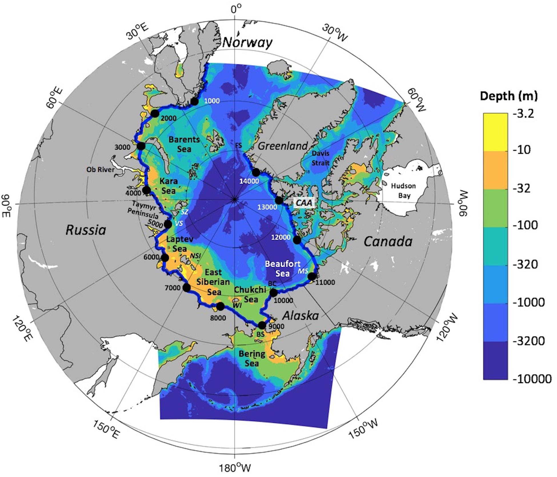
Figure 1. Map of the Arctic Ocean showing place names mentioned in the text and our model domain. Model depths (adapted from Jakobsson et al., 2012; Danielson et al., 2015) are shown with a log-based color shading. Black circles labeled in increments of 1000 show distances in km along the coastal transect (x_ct) starting at the model boundary on the west coast of Norway (blue line). Abbreviations include: BC = Barrow Canyon, BS = Bering Strait, CAA = Canadian Arctic Archipelago, FS = Fram Strait; MS = Mackenzie Shelf, NSI = New Siberian Islands, SZ = Severnaya Zemlya, WI = Wrangel Island, VS = Vilkitsky Strait.

Islands delineate some of the shelf seas and represent semi-permeable boundaries between them. The Severnaya Zemlya archipelago separates the Kara and Laptev seas; the New Siberian Islands separate the Laptev and East Siberian seas; and Wrangel Island separates the East Siberian and Chukchi seas. The Canadian Arctic Archipelago is a topographically complex region in which frictional and scattering effects are both expected to play important roles; however, a detailed description of CSWs in this region lies beyond the scope of this study.

Wave Classification

Coastal trapped waves are a family of wave types whose dynamics depend upon density stratification, water depth and bottom slope, and the shape of the boundary (coast, shelf-break or other edge); see Wang and Mooers (1976); Brink (1991), Huthnance (1995). A subset of coastal trapped waves includes CSWs, which exhibit the characteristics of topographic Rossby waves in the presence of a vanishing coastal wall and a homogeneous water column (Buchwald and Adams, 1968; Wang and Mooers, 1976). Their generation is tied to the along-shore component of wind stress, which drives coastal set-up and set-down via cross-shelf Ekman transport (Adams and Buchwald, 1969; Gill and Schumann, 1974). CSWs can be expressed as the sum of multiple modes that each satisfy a wave equation (Clarke, 1977). The first mode of variability (Mode 1) often accounts for most of the coastal sea level changes at synoptic periods and, in the unstratified limit, Mode 1 approaches the case of a purely barotropic shelf wave (Gill and Schumann, 1974; Wang and Mooers, 1976), which is occasionally referred to as a coastal trapped surface Kelvin wave (Wang, 2003; Cushman-Roisin and Beckers, 2011). The phases of CSWs and surface Kelvin waves propagate cyclonically around closed systems such as the Arctic Ocean so that when viewed looking downstream, they propagate counterclockwise in the Northern Hemisphere with shallow water located to their right.

CSWs have frequencies (ω) that are smaller than the local inertial frequency (f; Figure 2), and their length scales are much greater than the shelf bottom depth (H). Along-shelf dimensions are typically set by the scale of the wind forcing (of order 10³ km) and the dispersion relationship. Their cross-shelf length scale is the smaller of the shelf width (L) or the barotropic Rossby radius of deformation, $R_{bt}=f^{-1}\sqrt{gH}$, where g is gravitational acceleration. CSW phase speed (“celerity”) c_p = ω/k is defined as frequency per wavenumber (k), while energy travels with the group velocity, c_g = dω/dk. Wavelength λ = 2π/k so that R_btk = 1 denotes a wavelength that is 2π greater than the Rossby radius. Dispersion relations (Cushman-Roisin and Beckers, 2011) delineate differing wave types and behaviors. Kelvin waves are non-dispersive (meaning that different wavelengths all travel at the same speed) and have a frequency directly proportional to the wavenumber; i.e., ω = fkR_bt. The CSW dispersion relation can be expressed in terms of a uniform bottom slope, α,

FIGURE 2

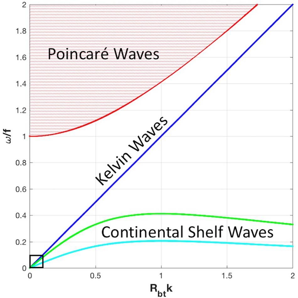
Figure 2. Dispersion relationships for surface Kelvin waves (blue), the continuum of Poincaré waves (red), and continental shelf waves (CSWs) for uniform bottom slopes of α = 1 × 10^–4 (cyan) and 2 × 10^–4 (green). The portion of the dispersion relationship for the focus of this paper is located close to the origin, within the black box.

$\mathrm{\omega }=\mathrm{\alpha }g{f}^{-1}k/[1+R_{bt}^2{k}^2](1)$

In the portion of the spectrum where the CSW frequency is small relative to the local inertial frequency (e.g., for the case in Figure 2 with α ∼10^–4), CSWs are only weakly dispersive (spreading of differing wavelengths and frequencies is minimal) and their character nearly merges with that of the surface Kelvin wave as R_btk approaches zero. The maximum frequency for CSWs occurs at R_btk = 1 and the group velocity changes sign on either size of this critical wave number (k_c). For wave numbers smaller than k_c, phase and energy propagate in the same direction; for shorter wavelengths, energy propagation opposes the direction of phase propagation; see a discussion of Antarctic CSWs by Marques et al. (2014).

Variations in shelf width and depth around the coastal perimeter affect CSW propagation, amplitude, wavelength, and speed characteristics. For the shallow Arctic shelves with characteristic depths of 30−60 m (e.g., the East Siberian Sea), R_bt ∼125−175 km, while for deeper Arctic shelves (e.g., the Barents Sea) with a mean depth closer to 250 m, R_bt ∼360 km. Thus, the external radius of deformation is on the order of, or less than, the shelf width over the broad Arctic shelves but greater than the shelf width over the narrow Beaufort and Greenlandic shelves and narrow passages near islands. Our focus is on the portion of the dispersion curve where R_btk << 1 (denoted by the small box near the origin in Figure 2). For CSW phase speed on an infinitely wide shelf, R_btk approaches zero and Eq. 1 can be reduced to c_p = αgf⁻¹ for bottom slope α (Cushman-Roisin, 1994), although assumptions of a uniformly sloping and infinitely wide continental shelf do not hold exactly. The East Siberian Sea has an average bottom slope α of 60 m per 500 km, or about 1 × 10^–4, whereas α for the Barents Sea slope is about 230 m per 1000 km, or 2.3 × 10^–4; however, large bathymetric variations in the Barents Sea means that, locally, substantially larger bottom slopes can be found. At 72°N, c_p is thus on the order of 7−30 m s^–1 (600−3000 km day^–1). Surface Kelvin waves, restored by gravity, travel at the shallow water wave speed $c=\sqrt{gH}$, which, for speeds of 7−30 m s^–1, conforms to a range of water depths (5−100 m) that encompass the majority of the shallow Arctic shelves. Hence, the Arctic shelves have bottom slopes and seafloor depths that we expect to predetermine a bounded range of CSW phase speeds and wavelengths.

Beyond the adjustments of propagating CSWs determined by shelf geomorphologies and dispersion relations, the magnitude of wind-induced SSH response to wind stress depends on the relative orientation between the wind direction and the coastline, the shelf stratification, and the strength and duration of the wind forcing. Cushman-Roisin and Beckers (2011) provide a useful steady-state relation for a storm surge amplitude (A) in an unstratified water column; A ∼ L_Fτ(ρgH)⁻¹, where L_F is fetch length, ρ is water density and τ is wind stress. Storm surges, once set up, are associated with finite along-shelf length scales matching that of the wind forcing. Their pressure fields rapidly (on the order of one inertial period) seek geostrophic balance, developing along-coast flow. The associated currents and mass transport, in turn, raise the downstream surface elevation and in this fashion a CSW propagates away from the local forcing region of a storm surge, adjusting to depth changes in order to conserve energy and vorticity. Coastal divergence (sea level set-down) anomalies similarly propagate as free waves, but with currents oriented in opposition to the direction of the sea level anomaly propagation. Pickart et al. (2011) showed that the relaxation response to the cessation of upwelling winds along the Beaufort Sea continental slope results in both barotropic and baroclinic responses having phase speeds that match theory for the two wave types.

Bathymetric and coastline variations induce CSW damping, reflections, refractions, scattering, and phase changes. Scattering that induces zero group velocity maximizes local energy loss (Brink, 1980). Long and otherwise non-dispersive CSWs can become dispersive where wavelength becomes smaller than the bottom depth (Mysak, 1980). Poincaré waves (ω = [f² + gHk²]^1/2) represent a potential sink of energy for CSW scattering through a non-linear cascade of energy into high frequency motions (Melville et al., 1989). Irregularities in the Siberian coastline may scatter CSWs into high frequency super-inertial Poincaré waves (Mysak and Tang, 1974); an “inverse cascade” may also occur with Kelvin wave generation by multiple Poincaré waves impinging upon a coastline (Howe and Mysak, 1973). Impingement upon blocking coastlines can result in phase-changing reflections, while sudden narrowing of the continental shelf, such as near the confluence of the Chukchi and Beaufort Seas or in the Kara Sea near Vilkitsky Strait, can scatter a portion of the energy, trap some energy, and permit a portion of the energy to pass through, in the fashion of a bandpass filter (Wilkin and Chapman, 1987).

Linking the Shelves

Early descriptions of CSWs include observations from near the Australian coast (Hamon, 1966), the US West coast (Cutchin and Smith, 1973), and the US East coast (Mysak and Hamon, 1969). In the Arctic, CSWs have proved useful in describing synoptic flow variations in the Barents and Kara Seas (Calafat et al., 2013; Drivdal et al., 2016) and in the Pacific sector of the Arctic (Pickart et al., 2011; Danielson et al., 2014). Conditions are also favorable for CSWs to traverse the passages through the Canadian Arctic Archipelago and along the Greenlandic shelves, but we are aware of only one study describing their effects in these regions, Fukumori et al. (2015), who noted the potential of these locations as likely pathways for diverting coastally trapped wave energy southward.

For phase velocities c_p > 0 and group velocities c_g > 0, as occurs for R_btk << 1, the Beaufort continental shelves are downstream of the Chukchi Sea, which in turn is downstream of both the broad Siberian shelves to the west and the Bering Sea shelf to the south. Fram Strait represents the single major continental shelf discontinuity along the Arctic Ocean’s perimeter, indicating that the Barents Sea shelf is an upstream origin of circum-Arctic wave motions, and the east Greenlandic shelf is the downstream terminus. In the quasi-circular and semi-enclosed Arctic Ocean, cross-basin length scales (3000−4000 km) are of the same order of magnitude as horizontal length scales of large atmospheric low-pressure systems. Hence, a large Arctic storm has the ability to drive cross-shelf Ekman transport simultaneously across many degrees of longitude. Fukumori et al. (2015) pointed out that Ekman transport across the continental slope drives an out-of-phase SSH relation between the shelf and basin and that coastally trapped waves can account for some SSH variability at monthly and shorter time scales. Csanady (1997) noted that many studies document the along-shore progression of oceanic response to wind forcing but the identification of freely propagating signals in the ocean is much less common.

Local winds over the Pacific-sector Arctic continental shelves can account for 30−50% of the synoptic scale variability in the coastal region, while including time-lagged remote winds can increase the fraction of variance explained by 10−20% (Danielson et al., 2014; Weingartner et al., 2017; Fang et al., 2020). Using a 1-layer (two-dimensional barotropic) model of the Pacific Arctic forced only by wind, Danielson et al. (2014) showed that including the combined effects of locally generated storm surges and their associated propagating shelf waves provides a skilfull reproduction of observed current variations in Bering Strait (r² = 0.79 in winter months) for synoptic-band current fluctuations. That study highlighted the importance of CSW generation over both the Bering Sea and the East Siberian Sea shelves to flow variability in Bering Strait. Subsequent studies by Peralta-Ferriz and Woodgate (2017) and Okkonen et al. (2019) also highlighted the East Siberian Sea as a regionally important locus for wind forcing and potential CSW generation.

Here, we build on these prior results with a broader spatial characterization of Arctic CSWs, and show that shelf elevation, circulation, and dissipation fields can depend on upstream atmospheric forcings that are even more distant than those considered by previous studies. To demonstrate how shelf waves mechanistically link the circumpolar shelves, we employ tide gauge and oceanographic mooring data, atmospheric reanalysis data, and a combination of realistic hindcast and idealized numerical experiments using ocean model integrations.

The rest of this paper is organized as follows. Datasets and models are described in Section “Materials and Methods.” Results are in Section “Results and Discussion,” beginning with a set of model-data comparisons that demonstrate model fidelity in reproducing wind-driven SSH anomalies. We then seek evidence of CSW behavior in the observations and the model results, describe their behavior, and quantify propagation speeds and the fraction of energy lost as they propagate along the Arctic continental shelves.

Materials And Methods

In situ Data

We use hourly and 6-hourly SSH data from16 coastal tide gauges from Norway, Russia, Alaska, Canada, and Greenland, and 4 moored pressure gauges on the Laptev, Chukchi and Bering Sea continental shelves (Table 1). The pressure gauges are all from relatively short taut-wire subsurface moorings deployed in water depths of less than 60 m. Record lengths vary due to data availability at each site. Some Arctic tide gauge stations do not report for part of each winter due to ice and some have nearly complete records over our time frame of interest.

TABLE 1

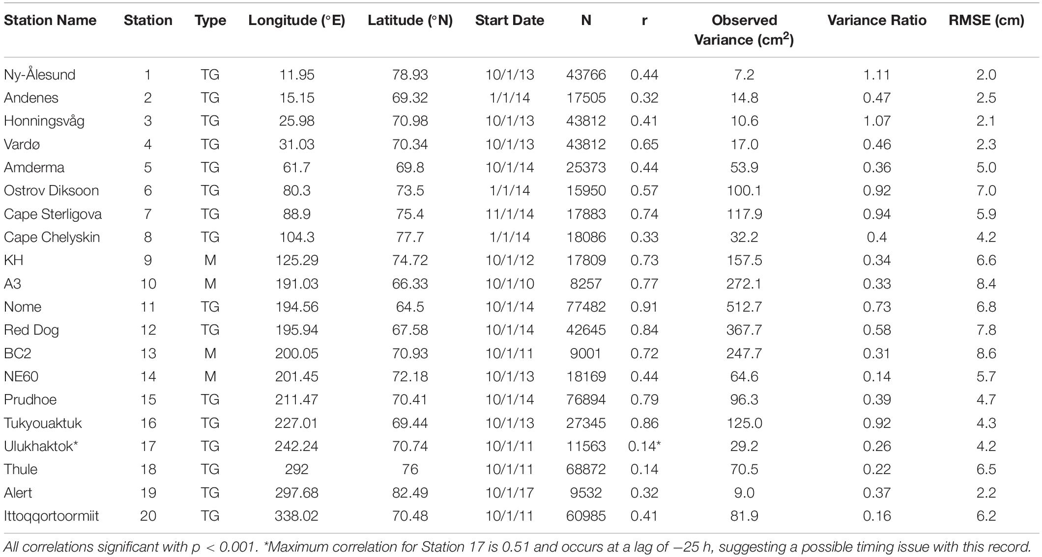
Table 1. Station name, number, station type (mooring = M, tide gauge = TG), location, start date for the band-passed time series records shown in Figure 4, total number of hours of model-data overlap (N) used for computation of correlation (r), variance of the observed record, ratio of modeled to observed variance, and the root mean square error (RMSE) between the model and observed records.

Seasonal, tidal, inertial and super-inertial fluctuations occur in frequency bands outside of our primary interests; unless otherwise stated, we focus on the synoptic time scale by bandpass-filtering the model and observational records using a 6th order phase-preserving Butterworth filter. A 1.5-day high frequency cutoff eliminates tidal (semidiurnal and diurnal) and inertial signals and an 11-day low frequency cutoff eliminates fortnightly signals associated with spring-neap tidal variability, and seasonal and interannual signals.

Atmospheric Reanalysis

We use the JRA55-do reanalysis (Tsujino et al., 2018) to characterize atmospheric conditions, force the ocean model described in Section “Ocean Model,” and correct the tide gauge and mooring data for the inverse barometer effect (Chelton and Enfield, 1986; Ponte, 2006). The JRA55-do reanalysis has been corrected in a manner similar to that of the Coordinated Ocean-ice Reference Experiment 2 (CORE2) effort (Yeager and Large, 2008) to be as self-consistent as possible for driving ocean models without flux biases. JRA55-do improves on CORE2 in that it has higher spatial and temporal resolution and is updated annually to provide the most recent year.

Ocean Model

For ocean hindcasts and idealized forcing experiments, we use the Regional Ocean Modeling System (ROMS), described by Shchepetkin and McWilliams (2005). ROMS is a free-surface, three-dimensional, hydrostatic primitive equation ocean circulation model that is based on a terrain-following, finite volume (Arakawa C-grid) configuration.

Our model implementation, which we refer to as the Pan-Arctic ROMS model (or PAROMS), is set up using ROMS options for high-order algorithms of tracer advection (3^rd order upwind in the horizontal direction and 4^th order centered in the vertical direction); surface and bottom boundary layers following the K-Profile Parameterization (Large et al., 1994); and atmosphere-ocean bulk flux computations based on the ocean model prognostic variables (Fairall et al., 2003; Large and Yeager, 2009). We employ a split integration approach, with slow and fast time steps of 60 and 3 s, respectively. The vertical coordinate system (50 layers) is based on terrain-following sigma-layers with finer resolution within the surface and bottom boundary layers. ROMS is coupled to a sea-ice model (Budgell, 2005) consisting of the elastic-viscous-plastic (EVP) rheology (Hunke and Dukowicz, 1997; Hunke, 2001), Mellor and Kantha (1989) thermodynamics, and frazil ice growth (Steele et al., 1989). Even though this sea ice model uses just one thermodynamic ice category, our Arctic simulations exhibit skillful results in the marginal ice zone (Danielson et al., 2011). PAROMS is implemented with a landfast ice parameterization that is based on estimates of basal stress as described by Lemieux et al. (2015).

The PAROMS domain (Figure 1) is configured for the Pan-Arctic region with a telescoping grid that stretches from south of the Aleutian Islands in the North Pacific (∼5 km resolution in the Bering Sea) to southern Greenland in the North Atlantic (∼8 km resolution in the Barents Sea). The telescoping grid was chosen for computational efficiency, minimizing the number of total grid points while maintaining the highest affordable resolution in the narrow Aleutian Island passes and Bering Strait. The bathymetry is a merged product that incorporates smoothed versions of the Alaska Regional Digital Elevation Model (ARDEM) version 2 (Danielson et al., 2015) and the International Bathymetric Chart of the Arctic Ocean version 3 (IBCAO; Jakobsson et al., 2012). Hudson Bay and the long Ob River estuary fall outside of the model domain and are truncated with closed model boundaries. The model surface forcing and terrestrial freshwater is based on the JRA55-do atmospheric reanalysis. Terrestrial freshwater, heat and volume fluxes are provided to the model through the coastal sidewall at all grid points, following a conservative mapping of the terrestrial discharge (Danielson et al., 2020) from the JRA55-do coastal runoff. Initial and boundary conditions are from the Simple Ocean Data Assimilation (SODA) for 1980−2015 (Carton et al., 2018) and global GOFS 3.0 HYCOM fields (Wallcraft et al., 2009) for 2015−2018. Inspection of model outputs across 2014−2015 shows a smooth transition between the boundary condition source change, so the relatively small differences in SODA and HYCOM reanalyses along the PAROMS boundary do not impact our results, which focus on shelf regions distantly located from the model edges.

While ROMS computes horizontal pressure gradients according to the equation of state, in our integrations model SSH fluctuations (ζ) do not include adjustments for atmospheric pressure or steric effects. Hence, to facilitate comparison we apply inverse barometer corrections (Chelton and Enfield, 1986) using the JRA55-do sea level pressure reanalysis estimates (−1 cm hPa^–1) to the observational data. We mostly constrain our model-data comparisons to fall and winter months when the Arctic shelf water column is not strongly stratified and steric effects are small.

An inner shelf transect (blue contour in Figure 1) is useful for evaluating PAROMS output and JRA55-do atmospheric forcing along the coast. The transect contour crosses estuaries and straits to better follow likely CSW propagation pathways. Distances along the contour are reported in kilometers beginning at the edge of the model domain on the west coast of Norway. Temporal bandpass filtering of model results is identical to that described above for mooring and tide gauge data and is applied to model outputs except where noted.

Model Integrations

We examine four sets of ocean model integrations in our study, which we designate integration groups A, B, C, and D. Integration A is a January 2010 to November 2018 PAROMS realistic hindcast that includes the setup and forcings described above in the “Atmospheric Reanalysis” and “Ocean Model” sections. The model writes hourly outputs of ζ and vertically averaged east and north velocity components (u and v, respectively) at all grid points. This hindcast is for direct comparison to the tide gauge and mooring data. A March 2017 breakpoint in the Integration A hindcast serves as the starting point for all Group B and Group C integrations.

Group B (Figure 3) is a set of integrations, each run over the same one-month period, with and without forcing from tides and the JRA55-do reanalysis winds. We leave the density structure to continue to drive slope boundary flows and other baroclinic flows throughout the domain. Baroclinic and non-tidal barotropic flows through the PAROMS Pacific and Atlantic boundaries remain, as does the perpetual Pacific-to-Arctic flow through Bering Strait. To minimize the effects of stratification and surface fronts, group B runs are initialized from a mid-winter breakpoint of integration A. Group B integrations help us isolate and identify the effects of wind forcing.

FIGURE 3

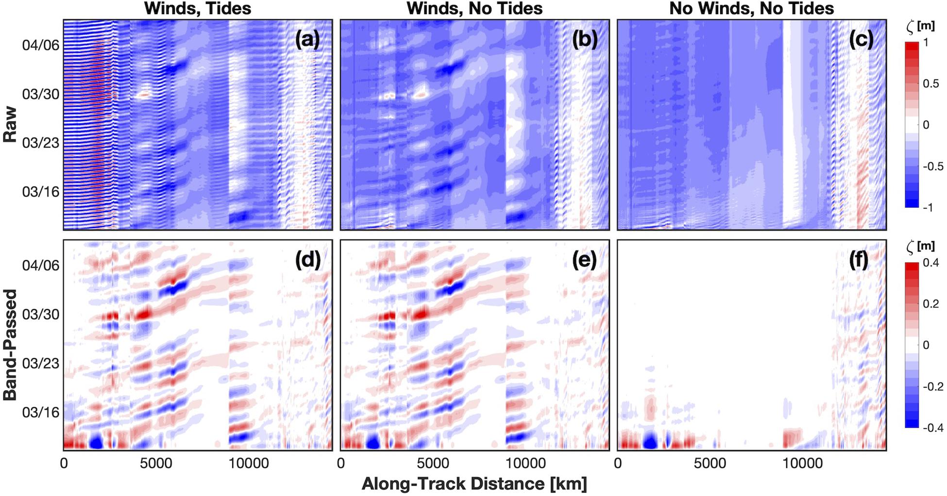
Figure 3. Group B integrations showing ζ (SSH variations) spanning 30 days in March and April 2017 along the coastal transect (x_ct) shown in Figure 1. The top row has raw, unfiltered ζ for three forcing conditions (a) with winds and tides; (b) with winds but without tides; (c) without winds and tides. The bottom row (d–f) isidentical to the top, except ζ is band-passed with a 6th order Butterworth filter between periods of 1.5-11 days. Note the different amplitude scales between the top and bottom row. The panels show that wind-forced signals can be well extracted from tidal and low frequency signals through band-pass filtering.

Integration Group C is a series of 22-day model runs begun from the same hindcast breakpoint (March 2017) as Group B, but under the influence of idealized wind forcing applied to isolated shelf regions. This approach allows us to examine the effects of propagating ocean anomalies after the idealized wind forcing is removed. Group C integrations begin with 5 days of no wind forcing to allow the inner shelf circulation and thermohaline fields time to adjust into unforced conditions (see Figures 3c,f). Following the spin-down, surface wind stress remains zero everywhere except for a localized patch of downwelling-favorable wind stress applied to one of the Arctic shelves. After the 5-day adjustment into unforced conditions, wind stress is smoothly ramped up from 0 to 0.14 N m^–2 (approximately 10 m s^–1) over the course of 2 days, held steady for 3 days and then ramped down again over the course of 2 more days. The imposed winds are favorable for coastal convergence via Ekman transport and applied only in shelf regions with seafloor depths less than 500 m. Following the cessation of wind forcing, the integrations then continue for an additional 8 days. We ran another integration for the full Group C 22-day time period without any wind forcing throughout, thereby providing a reference field that can be subtracted from the forced run to capture the anomaly response. Hourly outputs (depth-averaged velocity and sea level) from these integrations are subsampled (for data handling efficiency) to a regular grid spacing of 5° in longitude and 0.25° in latitude. We report zonal energy fluxes across the 5°-spaced meridional transects, which extend from the coast northward into the basin. For Bering Strait, we integrate the meridional energy flux across the east-west oriented strait; here, the model was not subsampled in order to maintain adequate lateral resolution.

Finally, we compute Integration D using reanalysis winds applied to an isolated portion of the Pacific Arctic shelf using a ROMS setup that consists of a 2-d (barotropic) model based on vertically integrated equations of motion as described by Danielson et al. (2014). This model run helps demonstrate the impact that distantly forced CSW signals can have on downstream adjoining shelves. Group C and Group D integrations were run with neither tides nor sea ice.

Results and Discussion

Separation of Signals

We first examine the behavior of modeled tide-induced and wind-induced SSH variations along the coastal transect (blue line in Figure 2). Hovmöller plots of the Group B integrations prior to temporal filtering (Figure 3) show that the synoptic-band influence of the wind can be readily separated from the higher frequency (e.g., tidal and inertial) signals. In addition, we find that wind forcing is primarily responsible for relatively large-amplitude (tens of cm) ζ signals that propagate anticlockwise along the Arctic coast. The speed (slope) of these propagating signals exhibits similarity through time more so than in distance along the coastal transect, suggesting that changes in speed are linked to spatially invariant properties such as the seafloor bathymetry.

The integration without winds and without tides (Figures 3c,f) shows a model e-folding spin-down time scale of about half a week. The spin-down is a result of starting from a solution forced by winds and tides that are subsequently turned off. The model exhibits some non-tidal high-frequency oscillations having large variance along the northern edge of the Canadian Arctic Archipelago (along-track distances of about 12,000−14,000 km). Investigation of this signal suggests that it is tied to boundary effects in southern Davis Strait and the complex bathymetry of the Archipelago.

Hindcast Model Performance

Using the integration A hindcast, we assess the ability of the 3-D PAROMS model to capture observed SSH fluctuations. We plot 3-month segments of normalized (unity variance, zero mean) time series of each filtered record and the corresponding model record (Figure 4 and Table 1). The normalization is implemented to highlight covariation similarities of the two signals. The skill of the model hindcast is quantitatively described by the correlation, variance ratio, and root mean square error (RMSE) given in Table 1. For most of the comparisons shown in Figure 4, we use three fall months (October through December) to minimize the influence of sea ice and stratification on the comparison results. For stations lacking a continuous 3-month record over October to December that overlapped with our model hindcast, we selected three other consecutive fall and/or winter months (Table 1).

FIGURE 4

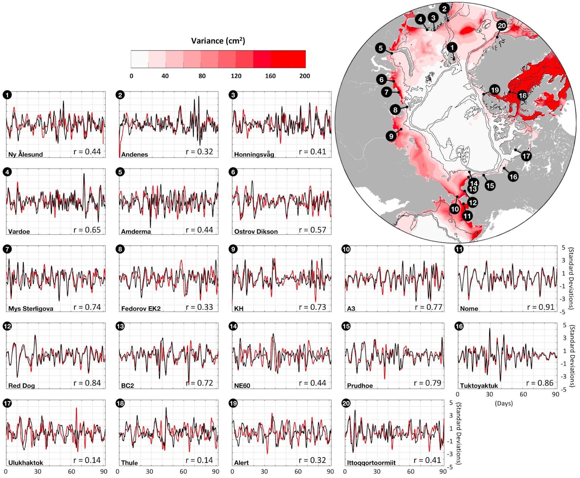
Figure 4. Station location map with color shading showing the modeled synoptic band sea level variance (cm²) and thin black contours at 60, 600, and 1800 m depths. Time series each show three months of observed (red) and PAROMS modeled (black) amplitude-normalized SSH variations in the synoptic band. Horizontal axis tick marks are spaced 10 days in time and vertical axis tick marks are spaced every 1 standard deviation. Time series start dates and amplitude variances are given in Table 1. The correlation coefficient shows the correlation for the entire period of record overlap between the model and the observations (not just the 3 months shown).

The model hindcast exhibits some fidelity in capturing synoptic event-scale fluctuations at all comparison sites, although it performs better at some than others (Figure 4 and Table 1). Across all of the stations, the mean variance ratio (52%) shows that the modeled synoptic-band amplitudes typically capture about half of the observed variance. Table 1 shows that the measured synoptic-band amplitudes are somewhat underestimated by the model at almost all comparison sites. Smaller correlations tend to be associated with reduced variances, reflecting the influence of signal-to-noise ratios. The average RMSE is 5.2 cm, with a standard error for this mean of 1.0 cm. The relatively deep Barents and Canadian Arctic Archipelago shelves show weaker model-data correlations, a behavior potentially linked to the following factors. First, the deeper shelves are more likely to remain stratified in fall and winter so the likelihood of a predominantly barotropic response at this time of year is less than on the shallower shelves. Second, sea level variability along the Norwegian coast is related in part to the variable magnitude of the along-slope North Atlantic current (Calafat et al., 2013). Third, the Barents Sea is located close to the energetic Icelandic Low atmospheric pressure cell, so SSH fluctuations imparted by the inverted barometer effect may be relatively larger than along the Siberian coast (Proshutinsky et al., 2001, 2004, 2007; Calafat et al., 2013) if the JRA55-do sea level pressure record is not perfect. We note that the maximum model-observation correlation coefficient occurs at 25 h for the Ulukhaktok station, suggesting a possible issue with the station data time stamp.

For the twenty stations shown in Figure 4, about one-third have a modeled synoptic-band variance that captures at least 50% of that observed, half are in the range of 30−50%, and the last few are between 10 and 30%. Sites #9, #10, #13 and #14 are mooring locations subject to some amount of current-induced tilt that impacts the pressure record; these four sites all have model variances that are fairly small in relation to the observations (13−35%). In contrast, within a few hundred kilometers of sites #10, #13 and #14, land-based tide gauge stations #11 and #12 show variance ratios of 0.58 and 0.73, respectively, suggesting that the underestimates of variance at sites #9, #10, #13 and #14 are likely tied more closely to mooring motion than to model inaccuracy.

Observed and model hindcast (Integration A) SSH fluctuations (Figure 5) over September 2011 to September 2013 at the KH mooring in the Laptev Sea (station #9 in Figure 4) demonstrate the model’s hindcast skill at a site with higher than average model-data correlation (r = 0.73, p < 0.001), RMSE (6.6 cm) and variance (157.5 cm²). The spectra (Figure 5e) show that the model’s frequency content well represents that of the KH observations over tidal, synoptic and seasonal time bands. Note that sub-inertial variability resolved by the model exhibits appreciable skill year-round (Figure 5b), even in the winter months when the Arctic environment is characterized by extensive pack and landfast ice cover.

FIGURE 5

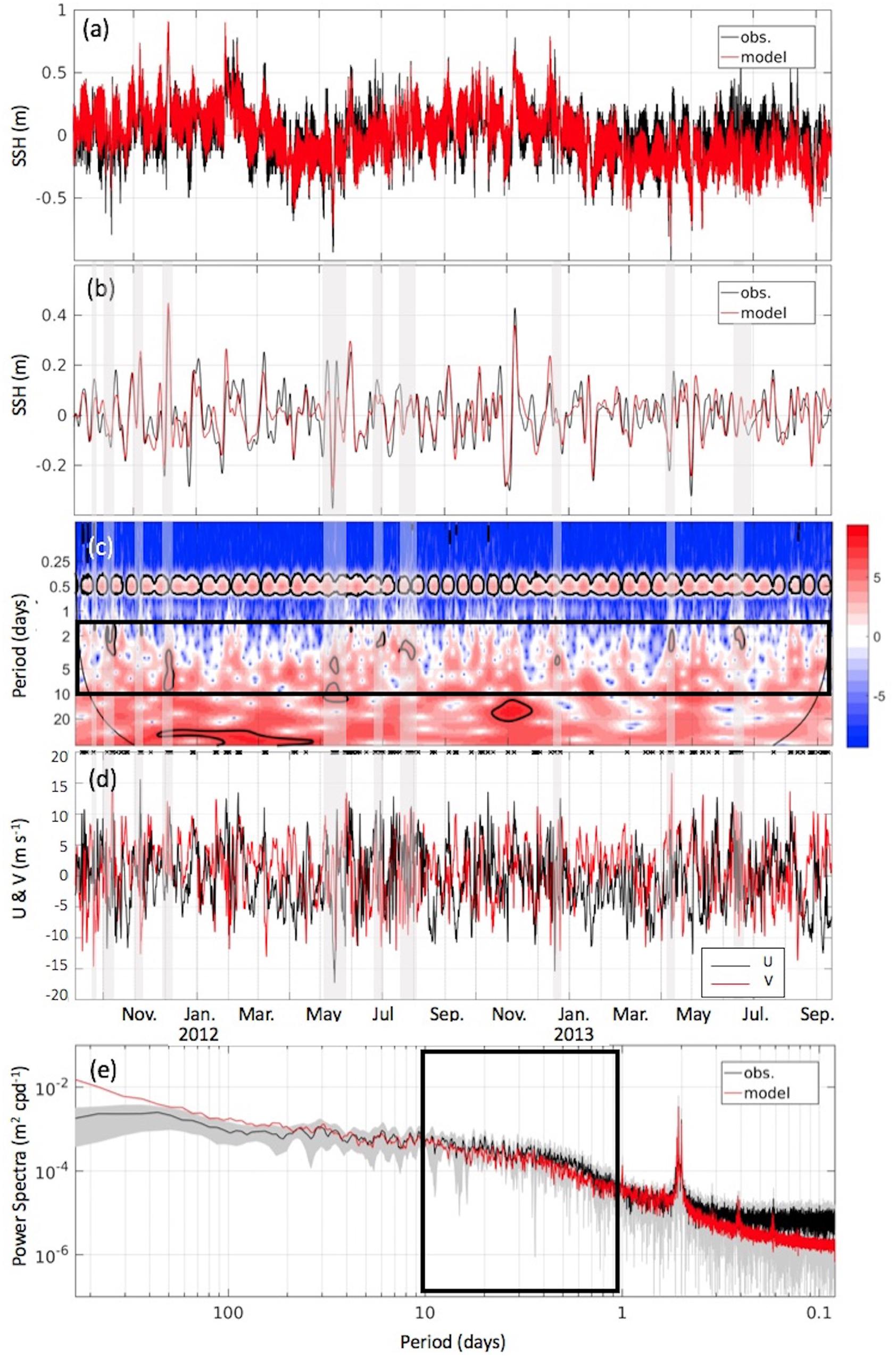
Figure 5. Site KH (site #9 in Figure 4) over September 2011–2013: (a) observed data (black) and modeled hindcast (red) raw time series; (b) 1.5 to 11 day bandpass filtered time series; (c) wavelet spectra (powers in units of normalized variance), (d) East-West (U, black) and North-South (V, red) raw (not filtered) wind components from JRA55-do at KH; (e) power spectra, smoothed with 5-point running mean filter and 95% confidence bounds on the observed spectra (shading). The confidence range on the model spectra is similar to that of the observed. Shading in panels (b–d) denotes the timing of synoptic scale peaks in the wavelet spectra. Thick black boxes in panels (c,e) denote the synoptic time scale in the spectra and wavelet plots. Small crosses at the top of panel (d) show instances of KH wind speed >10 m s^–1. Black contours in panel (c) show wavelet peaks that are significant at the 95% confidence level.

Spatial and Temporal Structure of the Arctic SSH Field

Having established the ability of the PAROMS model to reproduce the observed SSH variability at select observation stations with some fidelity, we turn next to a broader characterization of the pan-Arctic SSH field. In qualitative agreement with observed variances, the synoptic band modeled elevation variance is particularly high along the Alaskan coast in the Bering and Chukchi seas (Figure 4 map inset). The variance is notably high far from the shore in mid-shelf regions of the Laptev and East Siberian seas. We hypothesize that the elevated amplitudes along the Arctic Eurasian and Alaskan coastlines are associated with the effects of local wind forcing plus some contribution from propagating shelf waves. To confirm the hypothesis, we first demonstrate the existence of propagating anomalies in the ocean and then show that the signals are freely propagating waves and not merely the ocean’s response to propagating atmospheric storm systems. Based on prior studies, we expect a priori that most of the coastal anomaly response is driven by local wind forcing. Disentangling the ocean’s direct response from that of a propagating CSW may be difficult if storms translate along the shelf at a rate close the shallow water wave speed and in the same direction. Our approach herein is to tackle these two issues sequentially, beginning with analyses of the available observations and then turning to targeted model integrations.

Site KH in the Laptev Sea (station #9 on Figure 4) lies in a region of elevated SSH variability on the Eurasian shelf, at a location just upstream of where the shelf broadens and relatively high variances extend over 100 km offshore. The time-frequency distribution as resolved by wavelet analysis at this site (Figure 5c) shows numerous but intermittent high-amplitude events within the synoptic time scale. We find that the most energetic wavelet peaks (black contours in Figure 5c) in the synoptic time scale all coincide with instances of at least 10 m s^–1 in local wind forcing (e.g., December 2011; May 2012), but not all wind peaks of 10 m s^–1 (e.g., January 2012; March 2013) are associated with coincident wavelet energy maxima of similar magnitude. Instances of wind >10 m s^–1 are shown by crosses along the upper axis of Figure 5d. In winter, the KH location is often located close to the landfast ice edge (Janout et al., 2016), and this may affect the wind-current relation.

To test for the existence of eastward propagation of the hypothesized wave-like signal along the Arctic coastline, we computed lagged correlations using both observed and model data at KH (Station #9) relative to the upstream station at Cape Sterligova (#5) and downstream stations at NE60 (#14), Prudhoe Bay (#15) and Tuktoyaktuk (#16). We chose these stations based on the model’s skill at reproducing the local SSH variations (Table 1), spacing (to avoid adjacent stations being too close to demonstrate propagation), and overlapping of records in time. The comparison shows agreement between the model and observations, with fluctuations at Cape Sterligova occurring approximately 1 day before arriving at KH (Figure 6). On the downstream side, the maximal correlation occurs at about three to 4 days for site NE60, 4 to 5 days for Prudhoe Bay and 6 days for Tuktoyaktuk. The interval between the large negative correlations lying to either side of the zero-lag unity autocorrelation at KH is about 6 days for the model and 8 days for the observations, suggesting a time scale for the passage of one complete waveform at KH. The interval between the passage of a waveform based on peaks in the Figure 6 correlograms gives phase speeds of 9−13 m s^–1, or approximately 800−1100 km day^–1. Faster propagations are associated with the downstream side of station KH. This is consistent with a tendency for eastward-propagating CSWs velocity anomalies to associate with wider shelves and steeper seafloor slopes at the continental shelf break (shown in Section “Shelf Wave Effects” below).

FIGURE 6

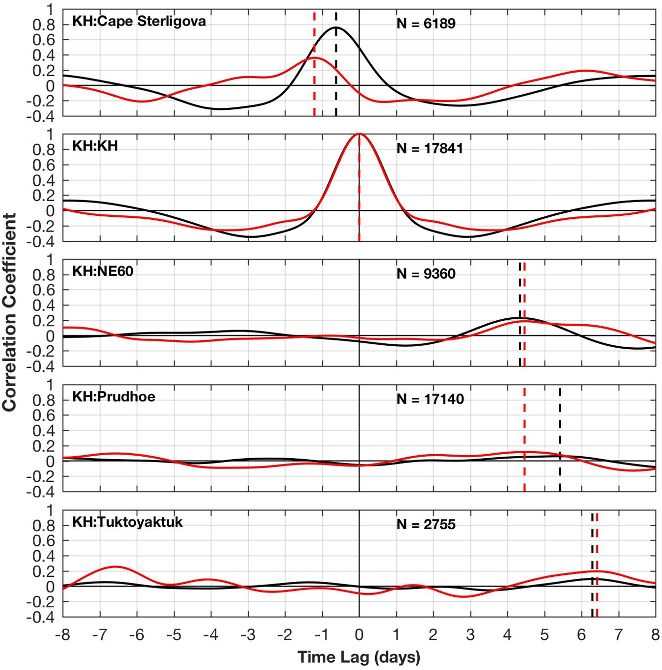
Figure 6. Lagged correlations relative to station KH of band-pass filtered observed (red) and band-pass filtered modeled (black) ζ anomalies. From top to bottom: Cape Sterligova, KH, NE60, Prudhoe Bay and Tuktoyaktuk. Relevant maxima are located with vertical dashed lines. The observed correlations are based on the maximum data record overlap without gaps between the two records, with the number of hours of overlap (N) denoted on each panel. The modeled correlations are based on the integration A hindcast using all record hours (N = 77,761). Spread of the black and red dashed lines suggests that uncertainty in the identification of the wave passage is generally less than a day. Uncertainty also depends on record length and ζ anomaly decorrelation time scales (2–6 days).

A dispersion relationship for the Barents and Kara seas (Figure 7) derived from one month (October 2014) of our filtered model output shows wave energy concentrated at periods near 2−6 days for wavelengths of 2000−7000 km, and at phase speeds of about 500−3000 km day^–1. These values fall within the range of the analytical solution for CSWs, suggesting that a substantial portion of the propagating energy in this particular month is indeed associated with CSW dynamics. Dispersion relationships for some other months show considerable energy existing at the smallest wavenumbers, suggesting that for these months the dominant response is not associated with CSWs but rather with faster-moving storm systems.

FIGURE 7

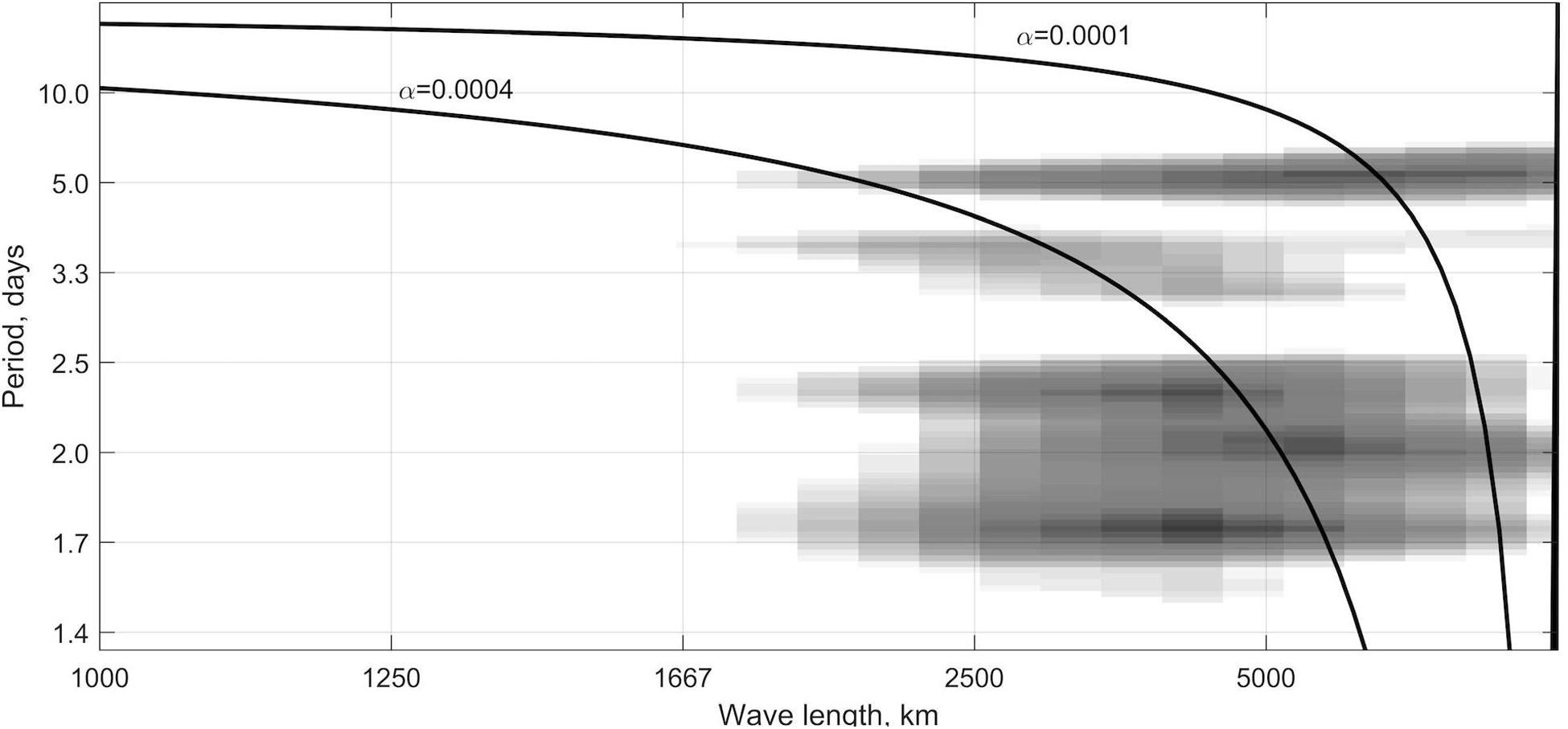
Figure 7. Two-dimensional power spectra (grayscale shading) calculated using PAROMS model hindcast results for the Barents and Kara Seas from one representative month (October 2014) along with dispersion curves (Eq. 1) for the continental shelf waves (CSWs; solid lines).

We constructed a time-lapse depiction of a canonical Laptev Sea shelf wave (Figure 8) by using site KH as a reference. Seeking to isolate strong signals in the synoptic band, we selected two standard deviations (+15 cm) at KH as a threshold. For all ζ anomalies at KH exceeding the threshold we averaged ζ anomalies across the whole Arctic at multiple time lags (spanning −3 to +5 days at one-day intervals). Over the 9-year model hindcast, we identified 104 positive ζ peaks at KH that exceeded two standard deviations (15 cm), or nearly one event per month on average. These events are seasonally skewed to late summer, fall and early winter months, with 65 of the 104 events occurring between August and January (Figure 9).

FIGURE 8

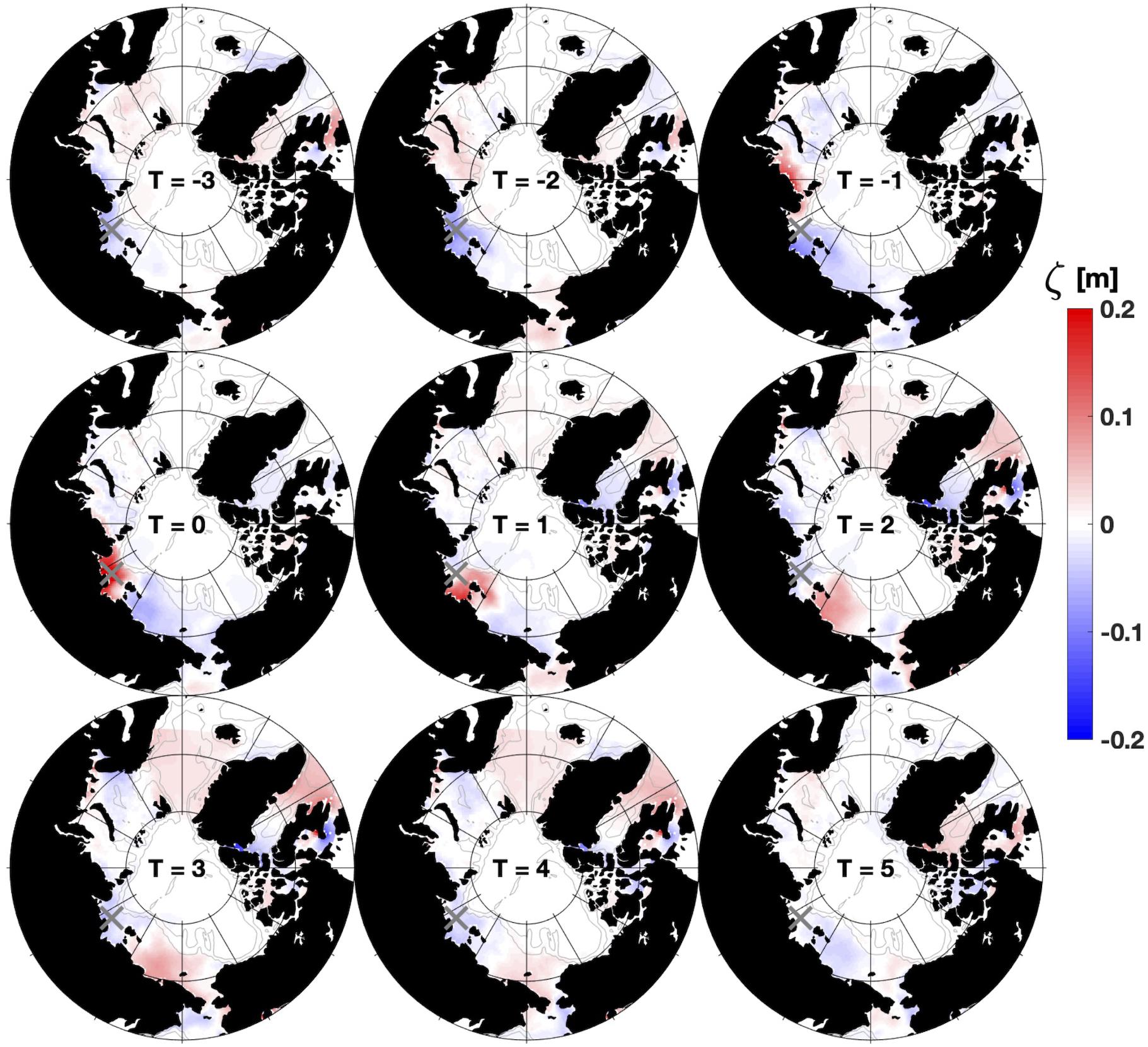
Figure 8. Compilation of PAROMS model hindcast results showing the pan-Arctic maps of the instantaneous ζ anomaly averaged at snapshot time lags of –3 to +5 days relative to ζ excursions that exceeded two standard deviations at site KH (marked with gray “X”). Averages are based on the 104 ζ > 2 standard deviation events in the 10-year hindcast.

FIGURE 9

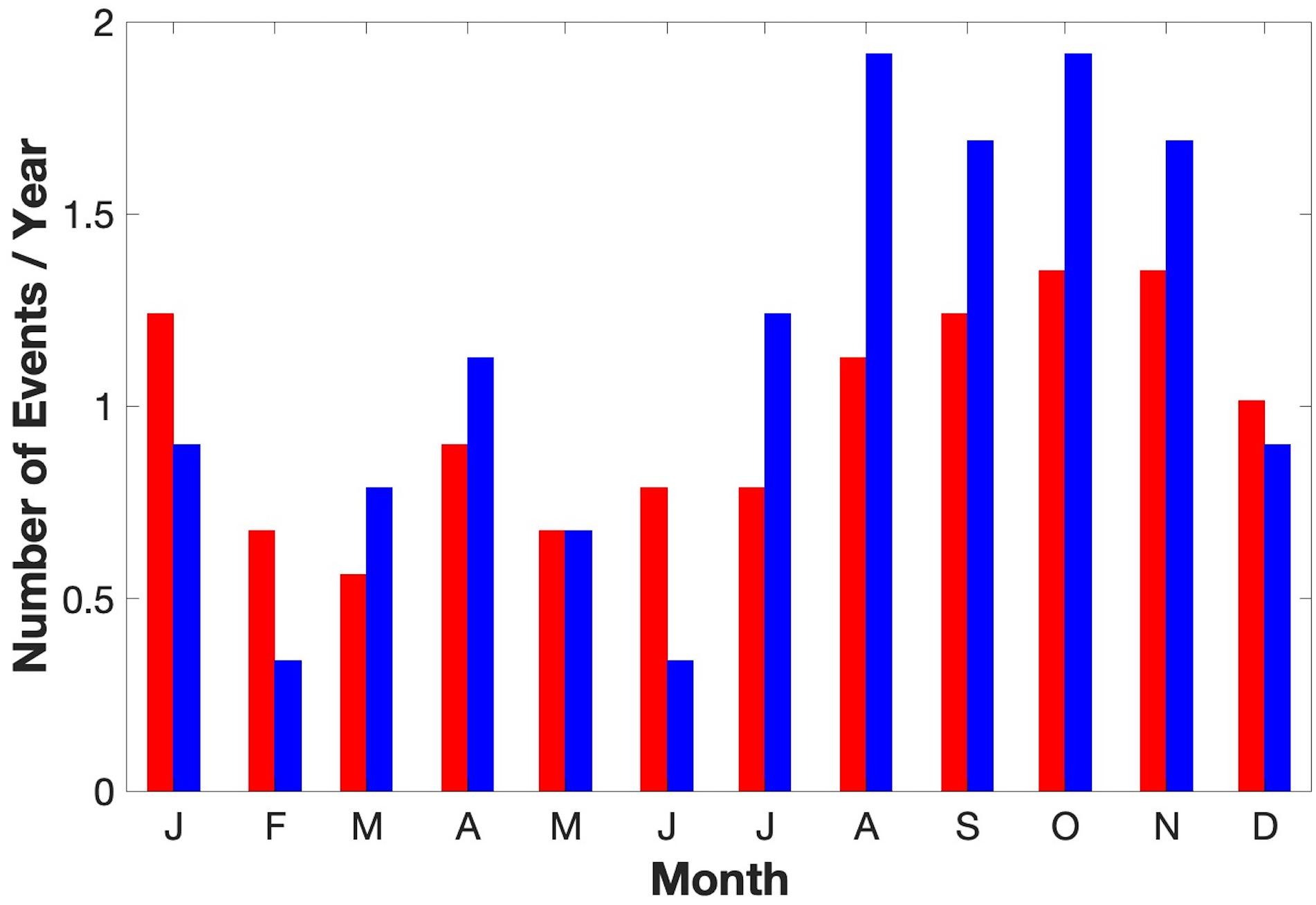
Figure 9. Monthly distribution of ζ > 2 standard deviation events per year for positive (red) and negative (blue) amplitude anomalies over the course of the 9-year model hindcast.

The first, weak, positive-amplitude ζ anomalies are observed over the Barents and Kara seas at lags of −3 and −2 days (Figure 8), followed by a stronger, coherent, and coastally enhanced anomaly in the Kara Sea at a lag of −1 day. The crest encompasses most of the Laptev Sea shelf at lag t = 0 (because site KH is the reference) and begins to enter the East Siberian Sea at lag + 1 day. Over lags +2, +3, and +4 days the crest crosses the East Siberian and Chukchi seas, and a portion passes southward through Bering Strait at lag +5 days. The ζ > 0 anomaly in Figure 8 extends across about 60 degrees of longitude, or about 800 km in along-shelf length. Note that the wave crest is preceded and followed by a negative anomaly trough. Such a trough is associated with the CSW and is also, in part, a consequence of zero-level offsets associated with the filtering operation. Bering Strait is about 2500 km and 3100 km from the New Siberian Islands and Vilkitsky Strait, respectively, so the canonical wave passing along the Siberian shelves exhibits a propagation speed of about 600−800 km day^–1, which closely matches the expected phase speeds estimated in the “Wave Classification” section above.

A comparison of wind and SSH fluctuations demonstrates the complex linkages between the atmospheric forcing and oceanic responses (Figure 10). Low pressure systems intrude into the Barents and Kara seas (near Figure 1 coastal transect distance x_ct = 5000 km) from the North Atlantic (x_ct = 0) on a regular basis, bringing wind and sea level pressure anomalies. Low pressure systems also propagate into the Arctic from the Pacific sub-Arctic near Bering Strait (x_ct = 9000). Propagating ocean anomalies also disappear in the vicinity of Bering Strait, either by escaping southward or by otherwise reflecting or dissipating.

FIGURE 10

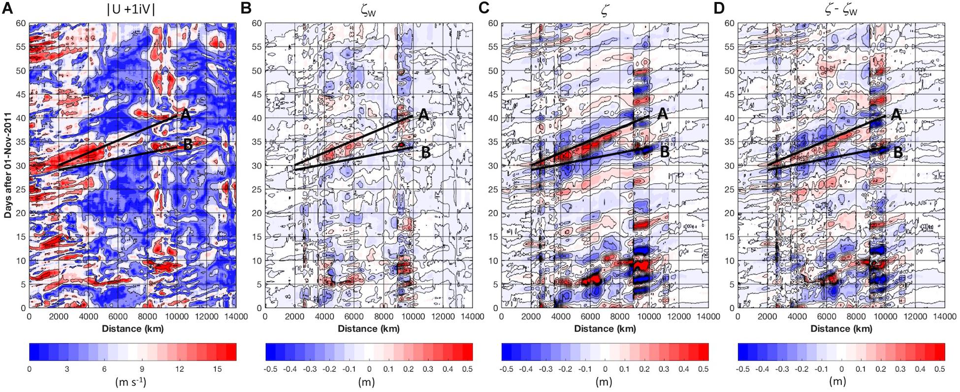
Figure 10. Sixty days (vertical axes) beginning November 01, 2011 along the coastal transect (horizontal axes, x_ct) shown in Figure 1 of panel (A) wind speed magnitude (m s^–1), (B) best fit regression (ζ_W = b₀ + b₁U + b₂V) of wind vector components U and V to the band-pass filtered ζ; (C) band-pass filtered SSH anomaly ζ, and (D) the estimated remotely forced SSH anomaly ζ -ζ_W. The black lines A and B denote along-shore propagation speeds of 800 and 1600 km day^–1, respectively. Slope of A best matches the ζ anomaly progression in panel (D) while the slope of B best matches the development of wind forcing in panel (A). For display purposes, amplitudes (C,D) have been clipped to –0.5 and 0.5 for values falling outside of this range.

Large-amplitude ζ anomalies (of either sign) in Figures 10, 11 are often associated with energetic local winds but our focus is on the more weakly propagating oceanic signals that extend beyond the time frame and spatial extent of surface wind forcing. For example, in Figure 10, wind was strong and favorable for coastal convergence in the Barents and Kara seas over days 30−35 but abated over days 35−40. This event set up height anomalies that propagated to at least x_ct = 9000 at a rate of ∼800 km day^–1 (line A in Figure 10). The slope of line B (∼1600 km day^–1) in Figure 10 matches the evolution of the wind forcing, while the slope of line A matches the progression of the ocean response.

FIGURE 11

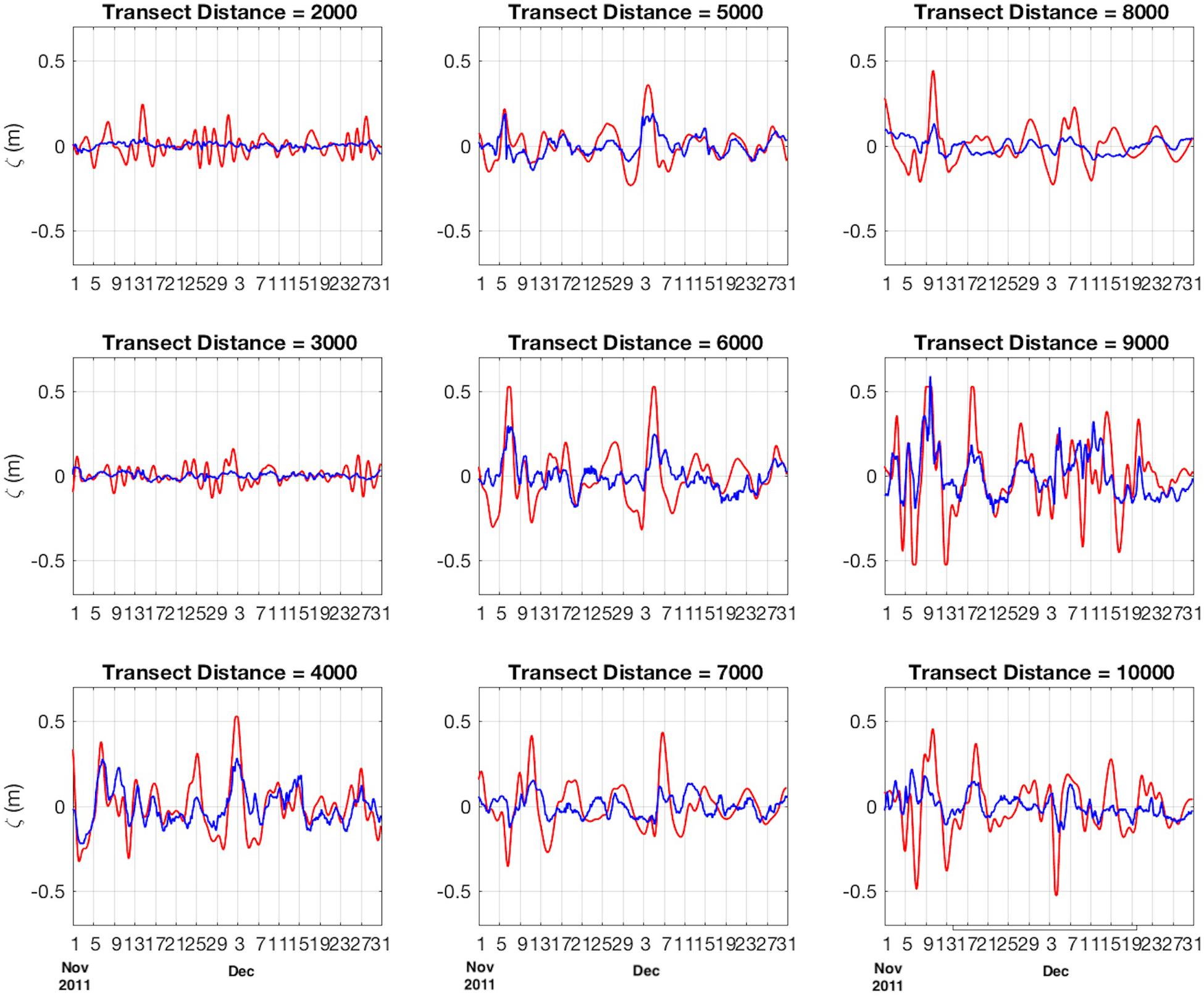
Figure 11. Bandpass-filtered time series of integration A modeled ζ (red) and the best-fit wind relation ζ_W (blue) at 1000 km intervals along the coastal transect (x_ct, Figure 1) beginning October 01, 2011.

Two notable features recur in the Chukchi Sea, where a distinct discontinuity in SSH variability persists through all months (Figure 10C). First, eastward-propagating waves often appear to undergo a 180-degree phase change as they impinge upon the Bering Strait region (near x_ct = 9000). Second, a “flattening” of the oceanic SSH anomalies consistently occurs between x_ct = 8,000 and 10,000 (Figures 3, 10). This feature reflects the effects of the coastline orientation: waves traveling eastward across the southern Chukchi Sea impinge upon the westward-facing Alaskan coastline nearly simultaneously for x_ct = 9,000 to 10,000, causing an apparent (but not real) local acceleration relative to the along-coast transect. Presumably, a transect along the continental slope would not depict such an acceleration.

Turning back to the Group B integrations (Figure 3), we note that, as expected for a shelf wave governed by seafloor depths (but not from storms propagating with bathymetrically unconstrained speed and direction), the band-passed results with wind forcing depicts propagating features that exhibit highly consistent phase speeds along much of the coastal transect: the propagating anomalies retain similarity in slope from one event to the next in both Figures 3, 10. Atmospheric storms are not constrained by ocean dynamics: while the wind Hovmöller plot (Figure 10A) shows temporally propagating wind forcing, the structure in the wind field is far less consistent than within the ocean field. The wind field (Figure 10A) shows both propagating events and near-stationary wind events (relative to the along-coast direction) that are persistent through time (e.g., days 45−60 at x_ct = 8000 to 10,000 near Bering Strait). It is difficult to explicitly separate the effects of propagating storm systems from propagating shelf waves in the realistic hindcast model of integration A; therefore, we now turn to a series of idealized numerical model integrations that allow us to better examine the nature of the CSW in isolation.

Shelf Wave Effects

Group C integrations (see the “Model Integrations” section) applied downwelling favorable wind (that triggers shoreward currents) to select shelf seas over the course of seven days. Beginning with an integration driven by easterly winds over the Kara Sea shelf, we sought evidence of propagating anomalies (Figure 12). The evolution of ζ and vertically averaged velocity anomalies, with anomalies computed as the forced integration minus the equivalent unforced Group C integration, depict the CSW signal confined to the shelf east of the forcing region (Figure 12). The ζ > 0 anomaly induced by the wind forcing propagated eastward at ∼1000−2000 km day^–1 and velocities were maximal near the shelf break. Velocity and ζ anomalies were strongest near the forcing region with values near 10−20 cm s^–1 and 10−20 cm, respectively. Magnitudes diminish with increasing distance from the forcing region; however, for integrations with wind stress applied to the Barents and Kara seas, speed anomalies up to 5 cm s^–1 were observed as far away as the Beaufort Sea. The imposed wind stress magnitude is common for Arctic storms and, while the integration is idealized, the magnitude of the response may be characteristic of storm events that persist for a few days.

FIGURE 12

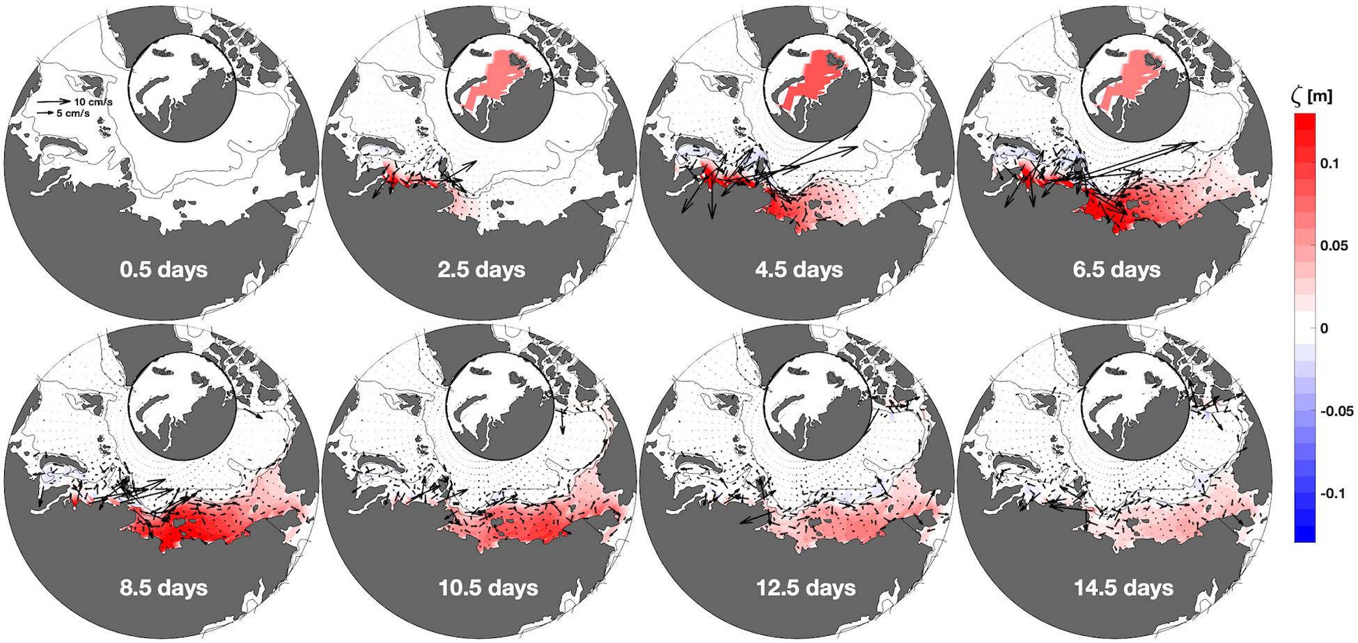
Figure 12. Difference between two model integrations, where one has no wind forcing and the other has an eastward surface wind stress with maximum amplitude of 0.14 N m^–2 induced over the Kara Sea (wind magnitude and location depicted in the small inset maps). Color in the main panels shows the ζ anomaly; vectors indicate barotropic velocity anomaly (see upper left panel for scale vectors). The plotted velocity vectors are spaced by 1° latitude for visual clarity. Time from the integration initialization is at the bottom of each panel. Wind stress begins at zero, ramps up during days 1–3 and ramps down to zero during days 6–8.

To quantify the fate of CSWs once they have propagated away from the source region, following Kowalik and Murty (1993) we estimated the zonal and meridional components of lateral energy flux as:

$F_x=\mathrm{\rho }uH[\mathrm{\zeta }g+{\mathrm{\hspace{0.33em}0.5}}^{*}(u^2+v^2)],(2)$

$F_y=\mathrm{\rho }vH[\mathrm{\zeta }g+{\mathrm{\hspace{0.33em}0.5}}^{*}(u^2+v^2)].(3)$

As with the patterns of barotropic velocity anomaly, energy flux is intensified near the shelf break and predominantly eastward (Figures 12, 13), consistent with the dispersion relationship (Eq. 1).

FIGURE 13

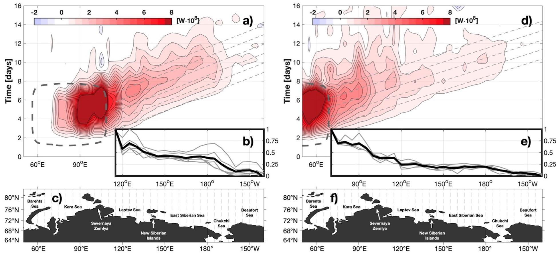
Figure 13. (a,d) Hovmöller plots of zonal energy flux (integrated over meridional lines), where red and blue represent eastward and westward propagation, respectively. Dark red colors include values above 8 × 10⁸ W. The vertical axis spans 16 days of model integration; the horizontal axis is longitude and aligns with the longitude axes in panels (b,e,c,f). The gray box denotes the spatiotemporal occurrence of the downwelling wind stress impulse in the Kara Sea (a,b,c) and the Barents Sea (d,e,f). The dashed lines correspond to a phase speed of ∼1900 km day^–1. (b,e) Gray lines show the integrated energy flux along the dashed lines in panels (a,d) and the black line is the ensemble average. Integrated fluxes are normalized to the maximum value in the zonal range, hence the vertical limits span 0 to 1. (c,f) A map of the major coastal topographic features along the zonal range. Dashed lines show the longitudes (5° spacing) over which total zonal energy is computed in panels (a,d,b,e).

We quantitatively assessed the evolution of CSW energy that propagates eastward across the shelves (Figures 13a,d), computing bulk zonal fluxes (F_tot, in Watts) (Figures 13b, 14B) by integrating the zonal energy flux (Eq. 2) across north-south transects (Figures 13c,f). For the group C integration with forcing in the Kara Sea (Figures 13a−c), the energy flux F_tot was a maximum of ∼10⁹ W at the eastern boundary of the forcing domain at t = 5 days. The decay was spatially non-uniform as the CSW propagated eastward. The energy flux dropped between the Laptev and East Siberian seas as the wave passed by the New Siberian Islands (∼130°E); there was a slower decline as it transited the East Siberian Sea, losing ∼10% of its energy prior to another large fractional decline in the Chukchi Sea (Figure 13b). By the time the CSW reached the coastal Beaufort Sea, the bulk zonal flux had declined by an order of magnitude to ∼10⁸ W. Over the broad, flat Eurasian shelves, away from islands, the decrease in eastward energy flux can be attributed to seafloor dissipation (there is no ice in the idealized integration C runs). In the Chukchi Sea, however, Bering Strait offers a southward pathway for losing Arctic-sourced wind energy (Eq. 3) to the sub-Arctic. The analysis shows that of the energy entering the Chukchi from the west, about half passes southward through Bering Strait and one quarter passes beyond Point Barrow into the Beaufort Sea, suggesting that the remaining quarter is dissipated locally (Figure 14).

FIGURE 14

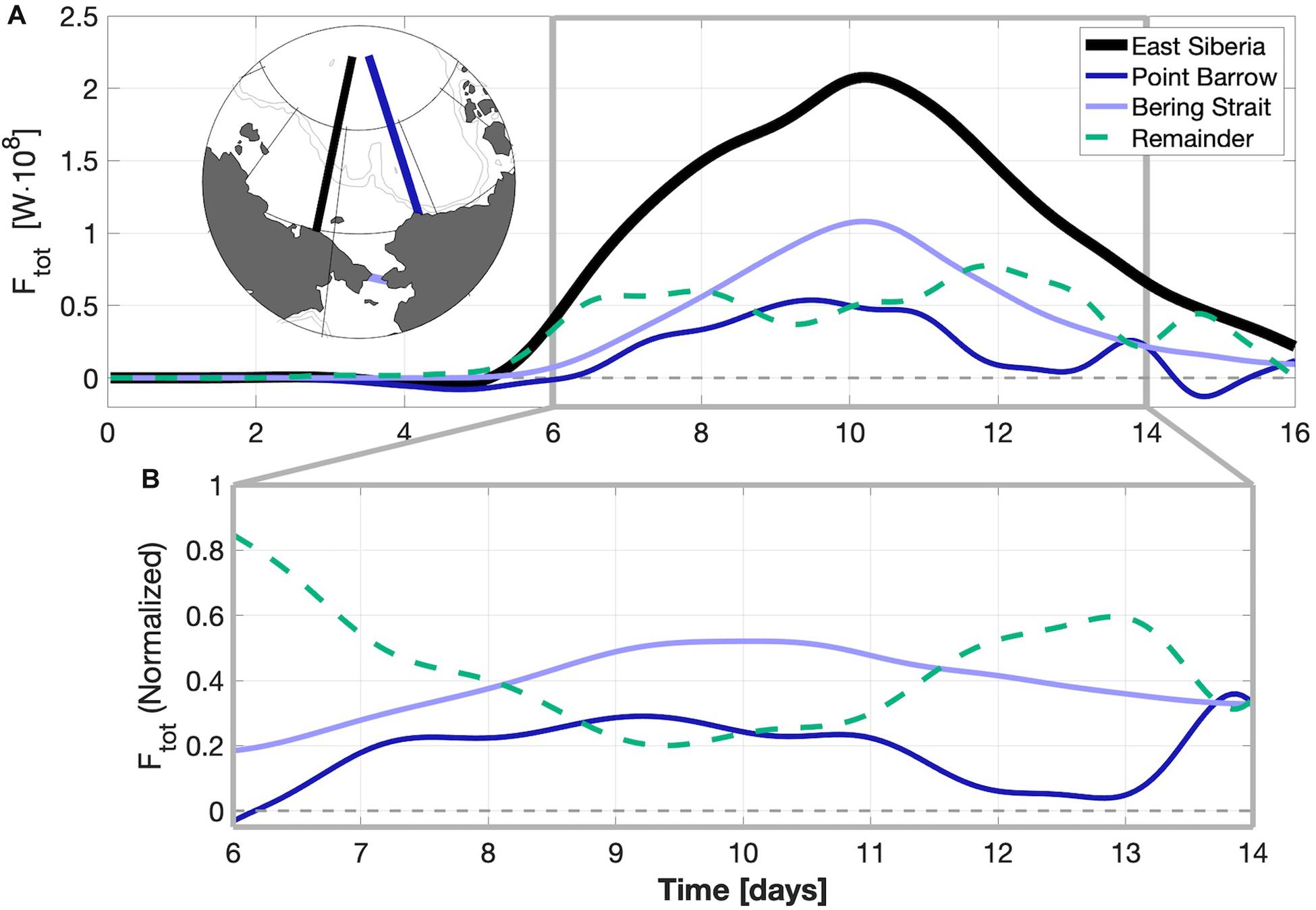
Figure 14. (A) Time series of integrated energy flux (F_tot) across the three transects shown in the inset map (East Siberia, Point Barrow, and Bering Strait) for the Kara Sea integration shown in Figure 12. The dashed line represents energy dissipation local to the Chukchi Sea: the difference between the CSW energy entering and leaving the region. The Point Barrow and Bering Strait time series are shifted by 14 and 10 h, respectively, to align the wave phases as they cross the integration transects. (B) Same as (A), but normalized by F_tot at the East Siberian line in order to highlight, fractionally, the pathways for CSW energy entering the Chukchi Sea.

For the Group C integration with wind applied over the Barents Sea (Figures 13d−f), we find that about half the eastward-propagating energy is lost near the Severnaya Zemlya archipelago and most of the remainder progresses onto the Laptev Sea either through Vilkitsky Strait or along the northern side of the archipelago. Energy fluxes lacking along-shore propagation tendencies appear as stationary tendrils that persist in time (e.g., near 90 and 110°E) in Figure 13d. These features may represent topographically trapped leakage of CSW energy into higher modes; they deserve future investigation and characterization.

We compare the magnitude of the CSW energy flux depicted in Figures 13, 14 with the mean northward flux of potential and kinetic energy carried by the Bering Strait throughflow. We applied the energy flux equation (Eq. 3) to the along-strait (northward) component of flow and integrated across Bering Strait (L = 85 km) with a typical flow of v = 0.3 m s^–1, a cross-strait sea level variation of ζ = 0.2 m and an average depth of H = 50 m. For Bering Strait, F_y ∼ 2.6 × 10⁹ (potential) + 1.2 × 10⁸ (kinetic) ∼2.7 × 10⁹ W. The vast majority (96%) of the total is due to the northward advection of potential energy. Under typical strong northward flow conditions (v ∼ 1 m s^–1) the kinetic energy flux increases by a factor of almost 40, while the potential energy flux increases by only a factor of three. Figure 14 suggests that the peak energy carried southward through Bering Strait by CSWs sourced in the Kara Sea can exceed the typical northward flux of kinetic energy in Bering Strait by a factor of two, but it remains an order of magnitude less than the typical total northward Bering Strait potential energy flux.

Wind-sourced power directly available for mixing can be expressed as P_W = δC_Dρ|W|³, where W is the wind speed (m s^–1), and the atmosphere-ocean drag coefficient C_D and coupling efficiency δ are typically each about 10^–3 (Simpson et al., 1978). For the Chukchi Sea (area ∼5 × 10⁵ km²), the net dissipation of a CSW sourced in the Kara Sea (∼0.5 × 10⁸ W; Figure 14) is unlikely to ever exceed that of local wind forcing, which is ∼5 × 10⁸ W for extremely weak winds of just W = 1 m s^–1. However, because CSW velocity anomalies are enhanced near the shelf break and in other regions of trapping, even shelf waves with distant origin may meaningfully contribute to local diapycnal mixing via bottom-stress induced turbulence.

Summary and Discussion

Our analyses show that the Arctic continental shelves are dynamically linked by propagating sea surface height and velocity anomalies associated with continental shelf waves (CSWs). The CSWs drive fluctuations in sea level and the currents in the coastal zone, near the shelf break, and in the vicinity of important chokepoints including Bering, Vilkitsky and Fram straits. The CSWs may play a role in climate-relevant processes such as mixing on the continental shelf and slope, and motion of sea ice. Although the effects are often less pronounced than impacts of locally forced diapycnal mixing (Rainville et al., 2011), ice motions (Spreen et al., 2011), or plume spreading (Bauch et al., 2011), they nevertheless represent an important remotely forced source of synoptic scale variability. The coasts of Norway and the Alaskan Bering Sea are sub-Arctic CSW generation sites from which wind-sourced energy propagates into the Arctic; channels of the Canadian Arctic Archipelago, Fram Strait, and Bering Strait represent pathways for Arctic-sourced CSW energy to escape the generally north-facing Arctic coastline.

The Arctic wind field repeatedly triggers new CSWs that propagate eastward to interact with the downstream elevation and flow fields, which are also under the influence of their own local winds and other forcing mechanisms. Therefore, it is difficult to analytically separate the effects of stationary local wind forcing, propagating wind forcing, and propagating oceanic responses. We have demonstrated that analyses of a combination of observational datasets and a range of numerical model simulations of varying forcing complexity allows us to at least partially decompose the synoptic Arctic SSH field into these different mechanisms. In situ (Figure 4) and model (Figures 4, 6, 8, 10, 12, and 13) data suggest that CSWs initiated over the Kara or Laptev seas may exert their influence over the course of at least 6 days.

Sea surface height variability caused by CSWs can impact longer-term (e.g., monthly) estimates of ocean mass and surface elevation derived from satellites operating with orbits that under-sample true ocean variability. Analysis of GRACE satellite and numerical model results suggests a basin-coherent dominant mode of SSH variability, representing about half of the variance, a secondary pattern that is a shelf-basin dipole, about one-fifth of the variance, and an even weaker pattern centered over the Barents Sea (see Volkov and Landerer, 2013; Peralta-Ferriz et al., 2014). The dipole feature appears consistent with phasing of the Arctic Oscillation and the Arctic Ocean geomorphology and thence to the associated wind field and Ekman dynamics. However, the relation between the monthly GRACE bottom pressure estimates and synoptic scale variations on the shelf is not fully clear because the GRACE data are adjusted (based on ocean modeling) to minimize the effects of aliased measurements (Landerer and Swenson, 2012; Cooley and Landerer, 2019), yet shorter-than-monthly variability appears to impact the monthly GRACE anomalies (Fukumori et al., 2015).

The shelves’ bathymetry variations, coastlines and islands trigger CSW wavelength and amplitude adjustments based on dispersion characteristics. To a lesser extent, changes in Coriolis parameter may also force wave adjustments, but variations in f are relatively small (1.33 × 10^–4 < f < 1.45 × 10^–4 s^–1) for the range of coastal latitudes between the Arctic Circle and the northern tip of Greenland. The broad Bering and Eurasian shelves are relatively flat; therefore, as suggested by Figures 13, 14, we expect that the effects of archipelagos and blocking coastlines will dominate the scattering of CSWs into higher modes.

SSH variability is important for safety and infrastructure protections associated with storm surge conditions, travel on landfast sea ice, contaminant spill responses and search and rescue efforts, all of which require knowledge of ocean current direction and speed. Regionally and locally driven storm surges are normally well anticipated and broadcast by forecasters, but propagating shelf waves are not necessarily considered in public forecast analyses or warnings of storm surge conditions due to the limited spatial extent of some forecast models, which can end at national or other arbitrary boundaries. Arctic subsistence hunting activities often use landfast ice as a platform for travel and staging (Gearheard et al., 2006) but the right combinations of ocean currents, winds, SSH anomalies and internal ice dynamics can trigger detachments of landfast ice. Landfast ice breakout events have surprised Indigenous hunters, with near-disastrous results for whale hunt participants near Utqiagvik, Alaska, in 1957 and 1997 (George et al., 2004).

As a final example of the potential magnitude of CSW effects in the eastern Chukchi Sea, we show results of the group D integration, a 2-D numerical model described by Danielson et al. (2014). This idealized model, based on vertically integrated equations of motion, is forced only by reanalysis winds over the Bering Sea. There is no mean background Bering Strait net throughflow and there is no wind applied over the Chukchi Sea. Hence, any flows detected in the Chukchi Sea are the result of northward-propagating CSWs that originated in the Bering Sea. The underlying bathymetry includes shelf isobaths that converge upon Barrow Canyon, which appear to focus the passing CSWs close to shore and accelerate the currents. Speeds exceed 20 cm s⁻¹ in both along-shore directions for the coastal convergent (Figure 15A) and the coastal divergent (Figure 15B) phases. Height anomaly magnitudes exceed 25 cm in the positive and negative directions for the coastal convergent and coastal divergent wave forms, respectively. Together, the amplitude and speed of these waves suggest their potential importance for landfast ice breakout events.

FIGURE 15

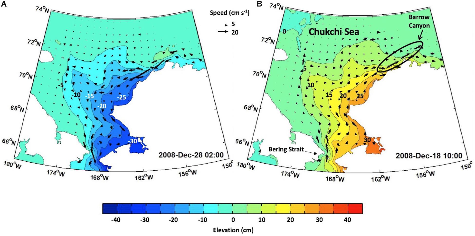
Figure 15. Two examples of Chukchi Sea CSWs generated south of Bering Strait using a 2-D ROMS model with wind stress only applied over the Bering Sea (Bering Sea not depicted on this map). Colors and contour labeling show SSH anomaly (cm). Note elevation anomalies of ±30 cm and currents reaching 20–30 cm s^–1. The location of Barrow Canyon is indicated in panel (B). Panel (A) shows an example of a sea level set-down associated with coastal divergence. Panel (B) shows an example of sea level set-up associated with coastal convergence.

Our hindcast model with full atmospheric and tidal forcing contains most of the physical processes required to represent the complex behavior of CSWs in the Arctic Ocean. However, we require more studies to disentangle the different processes so that we may move more closely to understanding how Arctic coastal trapped waves may change in future climates. These processes include the roles played by stratification, landfast ice, seasonality in storm events, regional differences, and their impact on other important processes such as diapycnal mixing. For example, we anticipate a high potential for wave-wave interactions in the Chukchi Sea where CSWs propagating from two different source regions converge. In the Canadian Arctic Archipelago, the complex coastlines and bathymetry undoubtedly reflect and scatter CSWs in interesting but presently unknown fashions. Seasonally changing stratification driven by ice melt and river discharge may alter wave type, behavior, and effects on ocean mixing and ice motion. As shown by Pickart et al. (2011), trapped waves at the shelf break propagating along the seasonal or permanent pycnocline are likely important components of the complete wave environments in these special regions. More accurate seafloor bathymetry grids will foster better model results, as will improvements to the atmospheric wind and pressure models that force the modeled ocean surface, and improvements to the representation of sea ice. Incorporating these additional complexities will improve the accuracy of models used for forecasting (for safety and marine operations considerations) and for assessing the overall response of the Arctic Ocean and sea ice as weather-band forcing changes in an evolving regional climate.

Data Availability Statement

JRA-55do model output is available from the Japan Meteorological Agency at: http://climate.mri-jma.go.jp/~htsujino/jra55do.html. SODA boundary conditions are available at: http://www2.atmos.umd.edu/~ocean/. HYCOM boundary conditions are available at: http://www.hycom.org. Tidal boundary conditions are available at: http://tpxo.net/. Most tide gauge data can be retrieved from public archives: the US National Oceanographic and Atmospheric Administration’s Tides and Currents archive (http://www.tidesandcurrents.noaa.gov), the University of Hawaii Sea Level Center (https://uhslc.woest.hawaii.edu/), the British Oceanographic Data Center Permanent Service for Mean Sea Level (http://www.psmsl.org) and the Fisheries and Oceans Canada Tides, Currents and Water Levels archive (http://tides.gc.ca/eng). Moored pressure records are available at: http://psc.apl.washington.edu/HLD/Bstrait/bstrait.html (A3), https://accession.nodc.noaa.gov/0160090 (BC2), and https://accession.nodc.noaa.gov/0163833 (HE60). PAROMS model outputs and other data products associated with this article are available at the Alaska Ocean Observing System (AOOS) online archive (http://www.aoos.org) under NPRB Project #1302. Model setup of the PAROMS ocean model is archived at doi: 10.5281/zenodo.3661518 and doi: 10.5281/zenodo.3708464

Author Contributions

SD conceived the study. KH ran all model integrations. SD, TH, and AP carried out analyses. All authors contributed to writing and/or provided datasets.

Funding

KF and MM were supported by the Ministry of Science and Higher Education of the Russian Federation (Project RFMEFI61619X0108). IP acknowledges support from the United States NSF grants (AON-1203473, AON-1724523, and AON-1947162), and the Norwegian Nansen Legacy program (project #276730) and Carbon Bridge program (project #226415) both funded by the Research Council of Norway. LP acknowledges support for the United States NSF grant OPP-1708424. SD, IP, and AP were supported by the United States NSF grant OPP-1708427. SD was also supported by the NPRB grants A91-99a and A91-00a. SD and KH acknowledge support from the North Pacific Research Board (NPRB) project 1302, National Science Foundation grant OPP-1603116, and Bureau of Ocean Energy Management grant M15AC 00011. MJ was supported by the German Federal Ministry of Education and Research (BMBF grants 03F0776 and 03G0833).

Conflict of Interest

The authors declare that the research was conducted in the absence of any commercial or financial relationships that could be construed as a potential conflict of interest.

The reviewer AR declared a past co-authorship with one of the authors MJ to the handling editor.

Acknowledgments

We thank Paul Wassmann for his leadership in Pan-Arctic knowledge synthesis efforts. We also thank the two reviewers for constructive comments that improved many aspects of the manuscript. We acknowledge all individuals responsible for generating moored, tide gauge, and model forcing datasets.

References

Aagaard, K., Weingartner, T. J., Danielson, S. L., Woodgate, R. A., Johnson, G. C., and Whitledge, T. E. (2006). Some controls on flow and salinity in Bering Strait. Geophys. Res. Lett. 33:L19602.

Google Scholar

Adams, J. K., and Buchwald, V. T. (1969). The generation of continental shelf waves. J. Fluid Mech. 35, 815–826.

Google Scholar

Bauch, D., Gröger, M., Dmitrenko, I., Hölemann, J., Kirillov, S., Mackensen, A., et al. (2011). Atmospheric controlled freshwater release at the Laptev Sea continental margin. Polar Res. 30:5858. doi: 10.3402/polar.v30i0.5858

CrossRef Full Text | Google Scholar

Brink, K. H. (1980). Propagation of barotropic continental shelf waves over irregular bottom topography. J. Phys. Oceanogr. 10, 765–778. doi: 10.1175/1520-0485(1980)010<0765:pobcsw>2.0.co;2

CrossRef Full Text | Google Scholar

Brink, K. H. (1991). Coastal-trapped waves, and wind-driven currents over the continental shelf. Annu. Rev. Fluid Mech. 23, 389–412. doi: 10.1146/annurev.fl.23.010191.002133

CrossRef Full Text | Google Scholar

Buchwald, V. T., and Adams, J. K. (1968). The propagation of continental shelf waves. Proc. R. Lon. Ser. A Mathem. Phys. Sci. 305, 235–250.

Google Scholar

Budgell, W. P. (2005). Numerical simulation of ice-ocean variability in the Barents Sea region: towards dynamical downscaling. Ocean Dyn. 55, 370–387. doi: 10.1007/s10236-005-0008-3

CrossRef Full Text | Google Scholar

Calafat, F. M., Chambers, D. P., and Tsimplis, M. N. (2013). Inter-annual to decadal sea-level variability in the coastal zones of the Norwegian and Siberian Seas: the role of atmospheric forcing. J. Geophys. Res. Oceans 118, 1287–1301. doi: 10.1002/jgrc.20106

CrossRef Full Text | Google Scholar

Carton, J. A., Chepurin, G. A., and Chen, L. (2018). SODA3: a new ocean climate reanalysis. J. Clim. 31, 6967–6983. doi: 10.1175/jcli-d-18-0149.1

CrossRef Full Text | Google Scholar

Chelton, D. B., and Enfield, D. B. (1986). Ocean signals in tide gauge records. J. Geophys. Res. Solid Earth 91, 9081–9098.

Google Scholar

Clarke, A. J. (1977). Observational and numerical evidence for wind-forced coastal trapped long waves. J. Phys. Oceanogr. 7, 231–247. doi: 10.1175/1520-0485(1977)007<0231:oanefw>2.0.co;2

CrossRef Full Text | Google Scholar

Cooley, S. S., and Landerer, F. W. (2019). GRACE L3-Produce User Handbook. Pasadena, CA: NASA Jet Propulsion Laboratory, 57.

Google Scholar

Csanady, G. T. (1997). On the theories that underlie our understanding of continental shelf circulation J. Oceanogr. 53, 207–229.

Google Scholar

Cushman-Roisin, B. (1994). Introduction to Geophysical Fluid Dynamics. Upper Saddle River, N.J: Prentice Hall, 320.

Google Scholar

Cushman-Roisin, B., and Beckers, J. M. (2011). Introduction to Geophysical Fluid Dynamics: Physical and Numerical Aspects. Cambridge, MA: Academic press.

Google Scholar

Cutchin, D. L., and Smith, R. L. (1973). Continental shelf waves: low-frequency variations in sea level and currents over the Oregon continental shelf. J. Phys. Oceanogr. 3, 73–82. doi: 10.1175/1520-0485(1973)003<0073:cswlfv>2.0.co;2

CrossRef Full Text | Google Scholar

Danielson, S. L., Curchitser, E. N., Hedstrom, K. S., Weingartner, T. J., and Stabeno, P. J. (2011). On ocean and sea ice modes of variability in the Bering Sea. J. Geophys. Res. 116:C12034. doi: 10.1029/2011JC007389

CrossRef Full Text | Google Scholar

Danielson, S. L., Weingartner, T. J., Hedstrom, K. S., Aagaard, K., Woodgate, R., Curchitser, E., et al. (2014). Coupled wind-forced controls of the Bering–Chukchi shelf circulation and the Bering Strait throughflow: ekman transport, continental shelf waves, and variations of the Pacific–Arctic sea surface height gradient. Prog. Oceanogr. 125, 40–61. doi: 10.1016/j.pocean.2014.04.006

CrossRef Full Text | Google Scholar

Danielson, S. L., Dobbins, E. L., Jackobsson, M., Johnson, M. J., Weingartner, T. J., Williams, W. J., et al. (2015). Sounding the Northern Seas: a New Western Arctic and North Pacific Digital Elevation Model. Eos 96, 13–17.

Google Scholar

Danielson, S. L., Hill, D. F., Hedstrom, K. S., Beamer, J., and Curchitser, E. (2020). Coupled terrestrial hydrological and ocean circulation modeling across the Gulf of Alaska coastal interface. J. Geophys. Res. Oceans JGRC24069. doi: 10.1029/2019JC015724

CrossRef Full Text | Google Scholar

Drivdal, M., Weber, J. E. H., and Debernard, J. B. (2016). Dispersion relation for continental shelf waves when the shallow shelf part has an arbitrary width: application to the shelf west of Norway. J. Phys. Oceanogr. 46, 537–549. doi: 10.1175/jpo-d-15-0023.1

CrossRef Full Text | Google Scholar

Fairall, C. W., Bradley, E. F., Hare, J. E., Grachev, A. A., and Edson, J. B. (2003). Bulk parameterization of air-sea fluxes: updates and modification for the COARE algorithm. J. Clim. 16, 571–591. doi: 10.1175/1520-0442(2003)016<0571:bpoasf>2.0.co;2

CrossRef Full Text | Google Scholar

Fang, Y. C., Weingartner, T. J., Dobbins, E. L., Winsor, P., Statscewich, H., Potter, R. A., et al. (2020). Circulation and thermohaline variability of the hanna shoal region on the northeastern chukchi sea shelf. J. Geophys. Res. Oceans e2019JC015639. doi: 10.1029/2019JC015639

CrossRef Full Text | Google Scholar

Fukumori, I., Wang, O., Llovel, W., Fenty, I., and Forget, G. (2015). A near-uniform fluctuation of ocean bottom pressure and sea level across the deep ocean basins of the Arctic Ocean and the Nordic Seas. Prog. Oceanogr. 134, 152–172. doi: 10.1016/j.pocean.2015.01.013

CrossRef Full Text | Google Scholar

Gearheard, S., Matumeak, W., Angutikjuaq, I., Maslanik, J., Huntington, H. P., Leavitt, J., et al. (2006). “It’s not that simple”: a collaborative comparison of sea ice environments, their uses, observed changes, and adaptations in Barrow, Alaska, USA, and Clyde River, Nunavut, Canada. AMBIO A J. Hum. Environ. 35, 203–211. doi: 10.1579/0044-7447(2006)35%5B203:intsac%5D2.0.co;2

CrossRef Full Text | Google Scholar

George, J. C., Huntington, H. P., Brewster, K., Eicken, H., Norton, D. W., and Glenn, R. (2004). Observations on shorefast ice dynamics in Arctic Alaska and the responses of the Iñupiat hunting community. Arctic 57, 363–374.

Google Scholar

Gill, A. E., and Schumann, E. H. (1974). The generation of long shelf waves by the wind. J. Phys. Oceanogr. 4, 83–90. doi: 10.1175/1520-0485(1974)004<0083:tgolsw>2.0.co;2

CrossRef Full Text | Google Scholar

Hamon, B. V. (1966). Continental shelf waves and the effects of atmospheric pressure and wind stress on sea level. J. Geophys. Res. 71, 2883–2893. doi: 10.1029/jz071i012p02883

CrossRef Full Text | Google Scholar

Henry, O., Prandi, P., Llovel, W., Cazenave, A., Jevrejeva, S., Stammer, D., et al. (2012). Tide gauge-based sea level variations since 1950 along the Norwegian and Russian coasts of the Arctic Ocean: contribution of the steric and mass components. J. Geophys. Res. Oceans 117:C06023.

Google Scholar

Howe, M. S., and Mysak, L. A. (1973). Scattering of Poincaré waves by an irregular coastline. J. Fluid Mech. 57, 111–128. doi: 10.1017/s0022112073001059

CrossRef Full Text | Google Scholar

Hughes, C. W., and Stepanov, V. N. (2004). Ocean dynamics associated with rapid J2 fluctuations: importance of circumpolar modes and identification of a coherent Arctic mode. J. Geophys. Res. Oceans 109:C06002.

Google Scholar

Hunke, E. C. (2001). Viscous–plastic sea ice dynamics with the EVP model: linearization issues. J. Comput. Phys. 170, 18–38. doi: 10.1006/jcph.2001.6710

CrossRef Full Text | Google Scholar

Hunke, E. C., and Dukowicz, J. K. (1997). An elastic-viscous-plastic model for sea ice dynamics. J. Phys. Oceanogr. 27, 1849–1868.

Google Scholar

Huthnance, J. M. (1995). Circulation, exchange and water masses at the ocean margin: the role of physical processes at the shelf edge. Prog. Oceanogr. 35, 353–431. doi: 10.1016/0079-6611(95)80003-c

CrossRef Full Text | Google Scholar

Jakobsson, M., Mayer, L., Coakley, B., Dowdeswell, J. A., Forbes, S., Fridman, B., et al. (2012). The international bathymetric chart of the Arctic Ocean (IBCAO) version 3.0. Geophys. Res. Lett. 39:L12609.

Google Scholar

Janout, M., Hölemann, J., Juhls, B., Krumpen, T., Rabe, B., Bauch, D., et al. (2016). Episodic warming of near-bottom waters under the Arctic sea ice on the central Laptev Sea shelf. Geophys. Res. Lett. 43, 264–272. doi: 10.1002/2015gl066565

CrossRef Full Text | Google Scholar

Kowalik, Z., and Murty, T. S. (1993). Numerical Modeling of Ocean Dynamics, Vol. 5. Singapore: World Scientific.

Google Scholar

Kowalik, Z., and Proshutinsky, A. Y. (1994). “The arctic ocean tides,” in The Polar Oceans and Their Role in Shaping the Global Environment, Geophysical Monograph 85, eds O. M. Johannessen, R. D. Muench, and J. E. Overland (Washington, DC: AGU), 137–158.

Google Scholar

Landerer, F. W., and Swenson, S. C. (2012). Accuracy of scaled GRACE terrestrial water storage estimates. Water Resour. Res. 48:W04531.

Google Scholar

Large, W. G., and Yeager, S. G. (2009). The global climatology of an interannually varying air-sea flux data set. Clim. Dyn. 33, 341–364. doi: 10.1007/s00382-008-0441-3

CrossRef Full Text | Google Scholar

Large, W. J., McWilliams, J. C., and Doney, S. C. (1994). Oceanic vertical mixing: a review and a model with a nonlocal boundary layer parameterization. Rev. Geophys. 32, 363–403.

Google Scholar

Lemieux, J. F., Tremblay, L. B., Dupont, F., Plante, M., Smith, G. C., and Dumont, D. (2015). A basal stress parameterization for modeling landfast ice. J. Geophys. Res. Oceans 120, 3157–3173. doi: 10.1002/2014jc010678

CrossRef Full Text | Google Scholar

Ma, B., Steele, M., and Lee, C. M. (2017). Ekman circulation in the A rctic O cean: Beyond the B eaufort G yre. J. Geophys. Res. Oceans 122, 3358–3374. doi: 10.1002/2016JC012624

CrossRef Full Text | Google Scholar

Marques, G. M., Padman, L., Springer, S. R., Howard, S. L., and Özgökmen, T. M. (2014). Topographic vorticity waves forced by Antarctic dense shelf water outflows. Geophys. Res. Lett. 41, 1247–1254. doi: 10.1002/2013gl059153

CrossRef Full Text | Google Scholar

Mellor, G. L., and Kantha, L. (1989). An ice-ocean coupled model. J. Geophys. Res. 94 10, 954.

Google Scholar

Melville, W. K., Tomasson, G. G., and Renouard, D. P. (1989). On the stability of Kelvin waves. J. Fluid Mech. 206, 1–23.

Google Scholar

Mysak, L. A. (1980). Topographically trapped waves. Annu. Rev. Fluid Mech. 12, 45–76. doi: 10.1146/annurev.fl.12.010180.000401

CrossRef Full Text | Google Scholar

Mysak, L. A., and Hamon, B. V. (1969). Low-frequency sea level behavior and continental shelf waves off North Carolina. J. Geophys. Res. 74, 1397–1405. doi: 10.1029/jb074i006p01397

CrossRef Full Text | Google Scholar

Mysak, L. A., and Tang, C. L. (1974). Kelvin wave propagation along an irregular coastline. J. Fluid Mech. 64, 241–262. doi: 10.1017/s0022112074002382

CrossRef Full Text | Google Scholar

Okkonen, S., Ashjian, C., Campbell, R. G., and Alatalo, P. (2019). The encoding of wind forcing into the Pacific-Arctic pressure head, Chukchi Sea ice retreat and late-summer Barrow Canyon water masses. Deep Sea Res. Part II Top. Stud. Oceanogr. 162, 22–31. doi: 10.1016/j.dsr2.2018.05.009

CrossRef Full Text | Google Scholar

Padman, L., and Erofeeva, S. (2004). A barotropic inverse tidal model for the Arctic Ocean. Geophys. Res. Lett. 31:L02303.

Google Scholar

Peralta-Ferriz, C., Morison, J. H., Wallace, J. M., Bonin, J. A., and Zhang, J. (2014). Arctic Ocean circulation patterns revealed by GRACE. J. Clim. 27, 1445–1468. doi: 10.1175/jcli-d-13-00013.1

CrossRef Full Text | Google Scholar

Peralta-Ferriz, C., and Woodgate, R. A. (2017). The dominant role of the East Siberian Sea in driving the oceanic flow through the Bering Strait—Conclusions from GRACE ocean mass satellite dataand in situ mooring observations between 2002 and 2016. Geophys. Res. Lett. 44, 472–411. doi: 10.1002/2017GL075179

CrossRef Full Text | Google Scholar

Pickart, R. S., Spall, M. A., Moore, G. W., Weingartner, T. J., Woodgate, R. A., Aagaard, K., et al. (2011). Upwelling in the Alaskan Beaufort Sea: Atmospheric forcing and local versus non-local response. Prog. Oceanogr. 88, 78–100. doi: 10.1016/j.pocean.2010.11.005

CrossRef Full Text | Google Scholar

Ponte, R. M. (2006). Low-frequency sea level variability and the inverted barometer effect. J. Atmos. Oceanic Technol. 23, 619–629. doi: 10.1175/jtech1864.1

CrossRef Full Text | Google Scholar

Proshutinsky, A., Ashik, I., Häkkinen, S., Hunke, E., Krishfield, R., Maltrud, M., et al. (2007). Sea level variability in the Arctic Ocean from AOMIP models. J. Geophys. Res. Oceans 112:C04S08.

Google Scholar

Proshutinsky, A., Ashik, I. M., Dvorkin, E. N., Häkkinen, S., Krishfield, R. A., and Peltier, W. R. (2004). Secular sea level change in the Russian sector of the Arctic Ocean. J. Geophys. Res. Oceans 109:C03042.

Google Scholar

Proshutinsky, A., Pavlov, V., and Bourke, R. H. (2001). Sea level rise in the Arctic Ocean. Geophys. Res. Lett. 28, 2237–2240. doi: 10.1029/2000gl012760

CrossRef Full Text | Google Scholar

Rainville, L., Lee, C. M., and Woodgate, R. A. (2011). Impact of wind-driven mixing in the Arctic Ocean. Oceanography 24, 136–145. doi: 10.5670/oceanog.2011.65

CrossRef Full Text | Google Scholar

Shchepetkin, A. F., and McWilliams, J. C. (2005). The regional ocean modeling system: a split-explicit, free-surface, topography-following-coordinate ocean model. Ocean Model. 9, 347–404. doi: 10.1016/j.ocemod.2004.08.002

CrossRef Full Text | Google Scholar

Simpson, J. H., Allen, C. M., and Morris, N. C. G. (1978). Fronts on the continental shelf. J. Geophys. Res. Oceans 83, 4607–4614. doi: 10.1029/JC083iC09p04607

CrossRef Full Text | Google Scholar

Spreen, G., Kwok, R., and Menemenlis, D. (2011). Trends in Arctic sea ice drift and role of wind forcing: 1992–2009. Geophys. Res. Lett. 38:L19501.

Google Scholar

Steele, M., Mellor, G. L., and McPhee, M. G. (1989). Role of the molecular sublayer in the melting or freezing of sea ice. J. Phys. Oceanogr. 19, 139–147. doi: 10.1175/1520-0485(1989)019<0139:rotmsi>2.0.co;2

CrossRef Full Text | Google Scholar

Tsujino, H., Urakawa, S., Nakano, H., Small, R. J., Kim, W. M., Yeager, S. G., et al. (2018). JRA-55 based surface dataset for driving ocean–sea-ice models (JRA55-do). Ocean Model. 130, 79–139. doi: 10.1016/j.ocemod.2018.07.002

CrossRef Full Text | Google Scholar

Volkov, D. L., and Landerer, F. W. (2013). Nonseasonal fluctuations of the Arctic Ocean mass observed by the GRACE satellites. J. Geophys. Res. Oceans 118, 6451–6460. doi: 10.1002/2013jc009341

CrossRef Full Text | Google Scholar

Volkov, D. L., Landerer, F. W., and Kirillov, S. A. (2013). The genesis of sea level variability in the Barents Sea. Cont. Shelf Res. 66, 92–104. doi: 10.1016/j.csr.2013.07.007

CrossRef Full Text | Google Scholar

Wallcraft, A. J., Metzger, E. J., and Carroll, S. N. (2009). Software Design Description for the Hybrid Coordinate Ocean Model (HYCOM), Version 2.2 (No. NRL/MR/7320–09-9166). John C. Stennis Space Center, MS: Naval Research Lab Stennis.

Google Scholar

Wang, B. (2003). “Kelvin waves,” in Encyclopedia of Meteorology, ed. J. Holton (New York, NY: Academic Press), 1062–1067.

Google Scholar

Wang, D. P., and Mooers, C. N. (1976). Coastal-trapped waves in a continuously stratified ocean. J. Phys. Oceanogr. 6, 853–863. doi: 10.1175/1520-0485(1976)006<0853:ctwiac>2.0.co;2

CrossRef Full Text | Google Scholar

Weingartner, T. J., Potter, R. A., Stoudt, C. A., Dobbins, E. L., Statscewich, H., Winsor, P. R., et al. (2017). Transport and thermohaline variability in B arrow C anyon on the N ortheastern C hukchi S ea S helf. J. Geophys. Res. Oceans 122, 3565–3585.

Google Scholar

Whitehouse, P. L., Allen, M. B., and Milne, G. A. (2007). Glacial isostatic adjustment as a control on coastal processes: an example from the Siberian Arctic. Geology 35, 747–750.

Google Scholar

Wilkin, J. L., and Chapman, D. C. (1987). Scattering of continental shelf waves at a discontinuity in shelf width. J. Phys. Oceanogr. 17, 713–724. doi: 10.1175/1520-0485(1987)017<0713:socswa>2.0.co;2

CrossRef Full Text | Google Scholar

Yeager, S. G., and Large, W. G. (2008). CORE.2 Global Air-Sea Flux Dataset. Boulder CO: Research Data Archive at the National Center for Atmospheric Research, Computational and Information Systems Laboratory.

Google Scholar