Large-Scale Variability of Physical and Biological Sea-Ice Properties in Polar Oceans

1. Introduction

Sea ice is one of the Earth system components most sensitive to climate change. Besides playing an essential role in global ocean circulation (e.g., Schmitz, 1995; Ferrari et al., 2014) and in regulating Earth's climate and weather (e.g., Liu, 2012; Dethloff et al., 2019), sea ice is crucial for the Arctic and Antarctic polar food webs (e.g., Eicken, 1992; McMinn et al., 2010; Meyer and Auerswald, 2014). Arctic and Antarctic pack ice serve as unique habitats for microalgae (Arrigo, 2014), which contribute to primary production and carbon transfer to higher trophic levels (Gradinger, 1999; Søreide et al., 2006; Budge et al., 2008; Fernández-Méndez et al., 2015; Wang et al., 2015, 2016; Kohlbach et al., 2016, 2017a,b, 2018; Schaafsma et al., 2017). Since light is the energy source of algae, the quantity and spectral composition of the light that penetrates the ice and reaches the surface ocean impacts primary productivity and biological activity at the bottom of the sea ice and below in the water column. Due to changes from complete darkness to 24 h daylight, and extreme natural variations in water temperature in high latitudes, the concentration of primary production in both the sea ice and the water column undergoes a seasonal cycle, which has a major impact on food availability and life cycle of animals living in polar regions (Swadling et al., 1997; Brierley and Thomas, 2002). Small organisms living inside or under the sea ice, and feeding on residing algae in (ice algae) or below (phytoplankton) it, transfer both ice-algae-produced and phytoplankton-produced carbon to the pelagic food web (Budge et al., 2008; Wang et al., 2015, 2016; Kohlbach et al., 2016, 2017a,b, 2018). Thus, knowledge of sea ice and under-ice environmental properties as drivers of large-scale patterns in the abundance and distribution of sea-ice algae and phytoplankton, and, consequently, of zooplankton and nekton, is essential for understanding ecosystem functioning and predicting possible consequences of climate change for the ecosystems (Flores et al., 2011, 2019; David et al., 2015, 2016; Ehrlich et al., 2020).

Sampling in polar regions is limited in space and time because of the harsh weather during most of the year and because of the remote and hard to access locations. Particularly for sea-ice algae, for which chlorophyll a (in the following abbreviated as chl a) is usually used as a proxy for their biomass, estimates are often based on a small number of ice core observations, which do not fully capture the patchiness and the spatial and temporal variability in their distribution (Miller et al., 2015; Lange et al., 2016, 2017b). Satellite remote sensing during the past decades has vastly improved, enabling large-scale monitoring of certain sea-ice parameters, such as sea-ice concentration and thickness. However, uncertainties of global satellite sea-ice concentration and thickness retrievals on smaller scales, e.g., in the range of a few kilometers, can reach the magnitude of the measurement itself (Ivanova et al., 2014; Ricker et al., 2015). Moreover, despite new satellite advancements (i.e., ALOS—Advanced Land Observation Satellite), resolving small scale features such as ridges is still a challenge due to the relatively large footprint. Satellite snow depth retrievals are under development, but further evaluation and validation are needed (Guerreiro et al., 2016). Furthermore, satellite measurements do not provide enough information for the study of in-ice and under-ice environmental characteristics. This is particularly true for ice algae and phytoplankton in ice-covered regions that cannot be observed by satellite so that a comprehensive picture of their distribution on large scales remains difficult to obtain. Therefore, non-disruptive time series of sea-ice algae are non-existent. Only recently, technological developments allowed the estimation of under-ice properties, including light and in-ice chl a, on the scale of hundreds of meters in the Arctic region (Nicolaus et al., 2012; Nicolaus and Katlein, 2013; Katlein et al., 2015, 2019; Lange et al., 2017b) and in the Antarctic (Arndt et al., 2017).

The effects of ice algae on the spectral distribution of light under the ice were first observed by Maykut and Grenfell (1975), followed by studies focused on investigating the wavelengths that are affected by the presence of algae (Legendre and Gosselin, 1991), and on distinguishing between effects of algae and snow on the spectral distribution of under-ice light (Perovich, 1990). Mundy et al. (2007) used, for the first time, normalized difference indices (NDI) for studying the effects of ice algae and snow on the under-ice hyperspectral measurements conducted under landfast first-year ice in the Canadian Arctic Archipelago. After comparing different methods for in-ice chl a retrieval, the NDI method was employed by Melbourne-Thomas et al. (2015) to estimate ice-algae biomass in two Antarctic regions, the Weddell Sea and off East Antarctica, and to retrieve in-ice chl a in the Weddell Sea in winter (Meiners et al., 2017). Lange et al. (2016) developed and compared different algorithms for the retrieval of ice algae in the Arctic pack ice during summer 2012, and applied such algorithms to under-ice hyperspectral measurements collected with under-ice profiling platforms (Lange et al., 2017b). For the first time, in this work these methods are applied to multi-annual data sets of under-ice hyperspectral measurements conducted over hundreds to thousands of meters, providing a unique large-scale study of the spatial variability of Arctic and Antarctic sea-ice algae biomass estimates.

In the present study, we present data collected with a Surface and Under Ice Trawl (SUIT) and used these data to characterize ice-associated environments in the Arctic Ocean and the Southern Ocean. We aim to provide a regional, and seasonal comparison of sea-ice properties on large scales in both Polar regions with a focus on: (1) under-ice water properties, (2) ice thickness, (3) light transmittance through sea ice and under-ice light, and (4) in-ice chl a estimates. Moreover, the spatial scale covered by the present data sets also allow for an (5) unprecedented investigation of the scales of variability for all the variables measured. Our account of the meter- to kilometer variability of structural and optical sea-ice properties should contribute to the validation and parameterizations of sea-ice models as well as habitat mapping in the polar oceans.

2. Data and Methods

2.1. Data

Data were collected during five campaigns in the Arctic Ocean and in the Southern Ocean, on board RV Polarstern (Figures 1, 2 and Table 1). In the Arctic Ocean, data were collected during early springtime (PS92, May-June 2015, Peeken, 2016), late springtime (PS106, June-July 2017, Macke and Flores, 2018), and during summer-autumn (PS80, August-September 2012, Boetius, 2013). In the Southern Ocean, the campaigns cover wintertime (PS81, August-October 2013, Meyer and Auerswald, 2014), and summertime (PS89, December 2014-January 2015, Boebel, 2015).

FIGURE 1

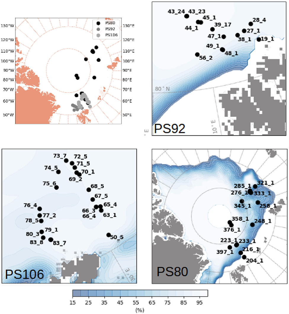
Figure 1. Map of the Arctic with the stations carried out during PS80 (summer-autumn 2012), PS92 (early spring 2015) and PS106 (late spring 2017). Ice concentration averaged over the period of sampling of each expedition was taken from OSISAF (EUMETSAT, 2011).

FIGURE 2

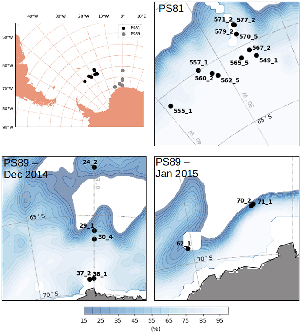
Figure 2. Map of the Antarctic with stations carried out during PS81 (winter 2013) and PS89 (summer 2014/2015). Ice concentration averaged over the period of sampling of each expedition was taken from OSISAF (EUMETSAT, 2011).

TABLE 1

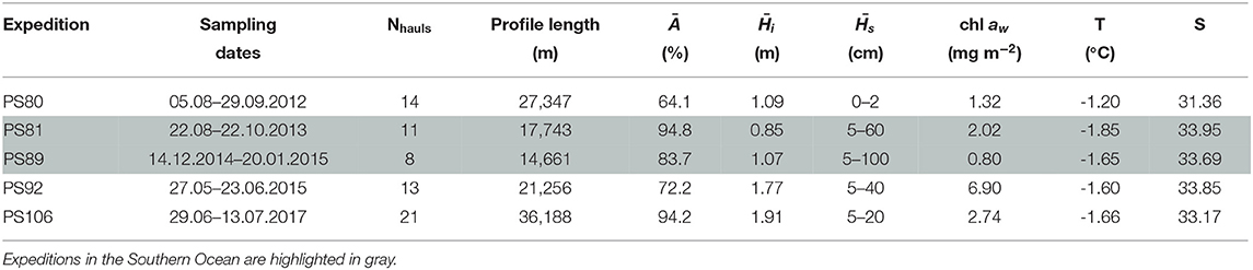
Table 1. Table with listed, for each expedition, the number of profiles considered in the analysis (N_hauls), the total profile length, the mean ice concentration (Ā), mean total ice thickness ($\overline{H_i}$) and mean snow depth ($\overline{H_s}$), under-ice water chl a (chl a_w) multiplied by the vertical section of the SUIT (2 m) to obtain integrated values, temperature and salinity.

Sampling was performed with Surface and Under Ice Trawls (SUIT, van Franeker et al., 2009; Flores et al., 2012). The SUIT consists of a steel frame with a 2 × 2 m opening and two 15 m long nets: a 7 mm half-mesh commercial shrimp net, and a zooplankton net with a 0.15 mm (PS106) or 0.30 mm (PS80, PS81, PS89, PS92) mesh. Floats attached to the frame keep the net at the surface or right at the sea-ice underside. An asymmetric brindle forces the net to tow off at an angle of approximately 60° so that it samples undisturbed sea ice away from the ship's wake. Previous studies using the SUIT nets have described in detail the ecological and biological aspects of the catch and distribution of organisms in both polar regions (Flores et al., 2011, 2012, 2019; David et al., 2015, 2016, 2017; Schaafsma et al., 2016, 2017). Since 2012 the SUIT is equipped with a sensors array (Lange et al., 2016, 2017b; Lange, 2017) developed in order to conduct coincident quantitative observations of the sea-ice and under-ice water environments. The sensors allow the direct observations of: (1) water inflow speed and direction, pitch and roll angles, and pressure (i.e., depth) using an Acoustic Doppler Current Profiler (ADCP; Nortek Aquadopp^® Profiler) with three acoustic beams, which allows 3-dimensional measurements of current velocities, at a frequency of 2 MHZ, and a sampling interval of 1 s; (2) water temperature, water salinity (practical salinity scale PSS-78; Fofonoff, 1985), and water depth by using a Conductivity Temperature Depth (CTD) probe (Sea and Sun Technology CTD75M memory probe) with a sampling interval of 0.1 s; (3) under-ice water chl a concentrations using a fluorometer (Cyclops, Turner Designs, USA) incorporated into the CTD; (4) distance from the ice surface by using an altimeter (Tritech PA500/6-E) incorporated into the CTD; (5) under-ice light levels using Ramses spectral radiometers (Trios GmbH, Rastede, Germany) with a wavelength range from 350 to 920 nm and a resolution of 3.3 nm. Incident solar radiation and under-ice irradiance were measured using an irradiance sensor (RAMSES-ACC) containing a cosine receptor with a 180° field-of-view. Under-ice radiance measurements were acquired using a radiance sensor (RAMSES-ARC) with a 9° field of view. As explained in detail in Lange (2017), the combined information from these different sensors allow also the retrieval of: (1) sea-ice draft derived by combining the CTD depth measurements with the distance from the ice (altimeter), and then corrected with pitch and roll measurements from the ADCP, as described in section 2.2; (2) ice-algal chl a derived from the Ramses spectral radiometers as described in section 2.4 (see also Table S1). Snow depth was recorded by visual observation of the ice under which the SUIT was traveling: A marked stick extending from the starboard side of the ship helps in quantifying the thickness of snow on top of the ice floes that are tilted during the ship passage. Part of these data have been used in previous works to study the relationship of environmental properties of sea-ice habitats with the community structure of sympagic fauna in the Arctic Ocean (PS80 and PS92, David et al., 2015, 2016; Schaafsma, 2018; Flores et al., 2019; Ehrlich et al., 2020), and in the Southern Ocean (PS81, Schaafsma et al., 2016, 2017; David et al., 2017), to develop and test algorithms for estimating in-ice chl a (PS80, Lange et al., 2016; Lange, 2017), to retrieve Arctic primary production on large scales in the Arctic summer (PS80 Lange, 2017; Lange et al., 2017b), and to estimate Arctic under-ice primary production based on under-ice irradiance measurements (PS92, Massicotte et al., 2019). All data collected during PS89 and PS106 are so far unpublished. Although data were collected during different years, this data set allows the investigation of differences between seasons in both the Arctic and the Antarctic, assuming that the sampling is representative of the season.

The profile lengths used for calculation of mean quantities (e.g., ice and snow thickness, water temperature and salinity, chl a in water and sea ice) correspond to the distance between the start and end trawl points, excluding parts of the profiles where the sensors data were unreliable due, for example, to sensors failure or damage. Thus, the profile length does not always correspond to the trawled distance, i.e., the total distance during which the net was towed in water by the ship, used to calculate the density of animals (e.g., David et al., 2017).

The sampled regions were different between expeditions: during Arctic spring (PS92 and PS106) data were collected north of Svalbard (Figure 1), in the latitudinal band between 80° N and 85° N. PS92 stations were located on the Yermak Plateau (lon <10° E, later referred to as Yermak stations), in the Sophia Basin and along the Svalbard shelf/slope (lon > 10° E, later referred to as basin & shelf stations). Some PS106 stations were also located in the Basin & shelf area (10° E < lon <20° E), the others were located between 20° E and 30° E. During Arctic summer (PS80), the sampling region extended toward the North Pole and to 130° E, thus covering the Nansen Basin and the Amundsen Basin. The two Southern Ocean expeditions (Figure 2) took place in the Weddell Sea, but at different latitudinal locations. During winter (PS81), data were collected between 52° S and 61.5° S. During summer (PS89), the Marginal Ice Zone (MIZ) had already retreated, forming a belt relatively close to the continent, and facilitating the sampling of southern areas (between 66° S and 69° S). During the southward trip in December 2014, the MIZ extended to ~66° S, during the return trip northward in January the MIZ had retreated to ~68° S. We will refer to the two different MIZs as Dec-MIZ and Jan-MIZ. In the period in-between the sampling of the two MIZs, the ship traveled through the inner pack-ice area that we will refer to as the pack-ice area.

2.2. Draft Calculation

Retrieval of the sea-ice draft makes use of the combination of depth h_w given by the pressure sensor of the CTD, distance from the ice h_a computed from the altimeter, and pitch β and roll ϕ movement of the SUIT:

$\begin{array}{ll}d=h_w-(h_a\times cos\beta \times cos\varphi )-h_{CTD}\times sin(\alpha +\beta ).& (1)\end{array}$

The CTD and the altimeter are connected but mounted in different parts of the SUIT, thus they are located at different depths. h_CTD is the distance between CTD and altimeter, α is the angle formed between the CTD probe, the CTD sensor, and the altimeter (see Figure 3 in Lange, 2017). In some cases, due to the failure of one instrument, the entire set of information was not available. In this case, we used the simplified version of equation (1) that does not include the pitch and roll correction:

$\begin{array}{ll}d=h_w-(h_a-h_{CTD}).& (2)\end{array}$

This is equivalent of assuming that the SUIT is towed perfectly parallel to the ice and, even if only an approximation, it has been proven reliable (R² = 0.78) in determining draft when the entire set of information was not available (Lange, 2017; Lange et al., 2017b). Handling of data gaps due to sensors malfunctioning or failure is explained in the Supplementary Material. Ice concentration for each profile was computed as the percentage of data points where ice thickness H_i was larger than zero. Ice thickness was computed by using a fixed density value (ρ = 0.917 g cm⁻³) for the sea ice. By doing this, final ice thickness values include both sea ice and snow, and we will refer to it as total thickness in the following (Lange et al., 2019). Mean and median thicknesses were computed for H_i > 0 and they include ridges. Keels of ridges were detected along each profile by using the Rayleigh criterion (Rabenstein et al., 2010; Castellani et al., 2014, 2015). A detailed analysis of the distribution and properties of ridges detected along each SUIT profile will be provided in a separate study.

During all expeditions, a helicopter-borne frequency-domain electromagnetic induction sounding system (EM-Bird) was used to measure the total sea-ice thickness (sea-ice thickness plus snow depth, Haas et al., 2009). The 4-m long EM-Bird was towed at a height of 10–15 m above the surface under a helicopter along mainly triangular flight tracks. With this method, the larger scale sea-ice thickness distribution can be observed also away from the ship track, which usually follows the easier sea-ice conditions in a region. Each triangle leg covered 15–30 nautical miles.

2.3. Under-Ice Light

Irradiance and radiance values were integrated over the Photosynthetically Active Radiation wavelength range (PAR; 400–700 nm). Since the SUIT does not always travel parallel to the ice but can encounter obstacles that make it swing, we included in the analysis only data with an inclination angle lower than 15° (Lange et al., 2017b). In order to reduce the effect of under-ice water between the actual position of the sensors mounted in the SUIT frame and the underneath side of the ice, we excluded all measurements associated with an altimeter value larger than 1.5 m following works by Katlein et al. (2015, 2016, 2017); Lange et al. (2016, 2017b).

Transmittance was calculated as the ratio between under-ice and incoming radiation, the latter measured with a Ramses sensor mounted on the ship's crows nest. Due to a sensor failure during summer 2012 (PS80) we used incoming global radiation data, which are obtained with a pyanometer, also placed in the same region as the above described sensor. For comparison, a regression between the two sensors was calculated for the simultaneous measuring period and gave excellent agreement. Thus, data from this were used to calculate transmittance values in September 2012. A detailed method used to obtain radiation values to cover this period can be found in the Supplementary Material.

The quantity of light reaching the underside of the ice layer is important for sea-ice algae and phytoplankton, as well as for sympagic fauna. In order to compare the amount of light between expeditions and sampling stations independently from the time of the day when we sampled, we calculated the insolation parameter as:

$\begin{array}{ll}{S}_i={\displaystyle {\int }_0^{24}}{I}_{h}T{R}_{i}dh,& (3)\end{array}$

where S_i is the insolation value (mol photons m⁻² d⁻¹) at position i along each profile, TR_i is the transmittance value at position i, and I_h is the modeled hourly incoming solar radiation (μmol photons m⁻² s⁻¹) above the surface (1°x1°spatial resolution, daily temporal resolution, interpolated hourly) based on the radiative transfer model SBDART (Ricchiazzi et al., 1998) as described in Laliberté et al. (2016). These data do not consider atmospheric parameters, such as cloudiness, which can affect the amount of radiation reaching the ship, where the incoming irradiance sensor is usually mounted. So defined, the insolation S_i is the amount of light passing through the bottom of the sea ice (i.e., PAR available for ice algae), at a specific position along the profile over an entire day. It is important to notice that the absence of information on cloud cover, or any other atmospheric parameter that could dampen the amount of light reaching the ice surface, potentially lead to overestimating the actual insolation values.

2.4. Retrieval of In-Ice Chlorophyll a

Since the retrieval of extensive spatial and temporal observations of sea-ice algae is limited in large part due to destructive techniques (i.e., based on the collection of sea ice from the field and subsequent melting and filtering of the ice), many studies in the past decades focused on estimating sea-ice algae based on under-ice hyperspectral measurements (Perovich, 1996; Mundy et al., 2007; Melbourne-Thomas et al., 2015; Lange et al., 2016; Meiners et al., 2017; Wongpan et al., 2018). In the present study, we employed normalized difference indices (NDIs) and Empirical Orthogonal Functions (EOFs) of under-ice spectra to estimate the concentration of chl a present in the ice. The heterogeneity of the environment covered by the present data set required the development of a specific algorithm for each expedition. The algorithms applied to the different data sets are listed in Table 2. For Arctic summer (PS80) data we used the EOF algorithm developed by Lange et al. (2016) based, amongst others, on the PS80 data set. Lange et al. (2016) recommended the EOF algorithm, instead of NDI, because it proved to be most reliable in catching the variability of in-ice chl a in the PS80 data set. For the Southern Ocean (PS81 and PS89) we used the NDI algorithm derived by Melbourne-Thomas et al. (2015) for the Weddell Sea. This algorithm was found to provide the most robust predictions of integrated chl a in comparison to others tested by Melbourne-Thomas et al. (2015). The NDI algorithm was developed based on summer data, and it is thus applicable to Antarctic summer (PS89). Meiners et al. (2017) applied the same algorithm to under-ice hyperspectral data collected with an ROV deployed during the Antarctic winter (PS81). Results showed that the algorithm provides a good fit with ice-core data collected during ice stations, we thus applied the same algorithm to the SUIT winter data (PS81). The NDI algorithm for Arctic spring (PS92 and PS106) was developed by comparison between coincident under-ice hyperspectral and in-ice chl a measurements of in total 8 ice stations carried out during the same campaigns. The accordance in sampling time (May-June-July), sampling region (Figure 1), and similarity of sea-ice properties (see section 3.2.1) justifies merging the data from these two spring expeditions. We used a total of 19 coincident measurements of under-ice irradiance and integrated chl a retrieved by measuring autotrophic pigments with High-Performance Liquid Chromatography (HPLC, for more details, see Tran et al., 2013). The NDIs for each wavelength pair were correlated with the integrated chl a values. Values lower than 0.1 mg m⁻² were excluded from the analysis. Correlation surfaces of normalized difference indices are shown in Figure 3A. We then used a linear model to explore the relationship between predicted chl a from the NDI algorithm and integrated chl a from the ice cores (Figure 3B). The NDI algorithm developed explains 60% of the variability (R² = 0.60).

TABLE 2

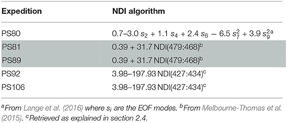
Table 2. Normalized Difference Indices and Empirical Orthogonal Functions algorithms used to retrieve in-ice chl a for the different expeditions.

FIGURE 3

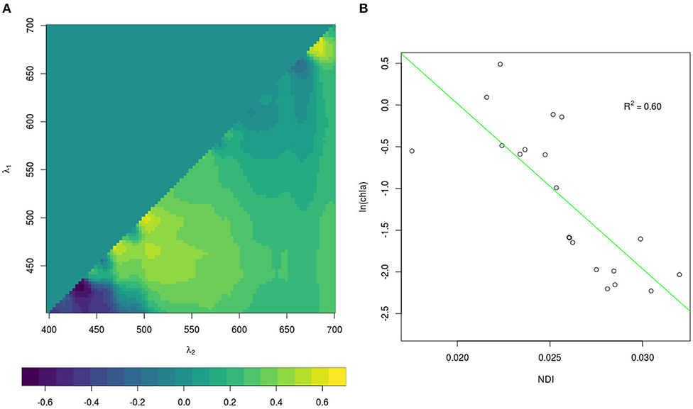
Figure 3. Correlation surfaces (A) of normalized difference indices for integrated chl a for PS92 and PS106. λ₁ and λ₂ are wavelengths pairs. Relationship (B) between observed normalized difference indices and integrated chl a (dots). The green line represents the fitted relationship given by the algorithm^c in Table 2.

An example of a SUIT profile including CTD data, retrieved ice draft, and retrieved in-ice chl a is shown in Figure 4. The sampling frequency of the RAMSES radiometers was lower than the one of the CTD and ADCP. In order to match ice thickness/draft with under-ice hyperspectral measurements, we computed averages of thickness and draft values falling between the beginning and the end of each light measurement.

FIGURE 4

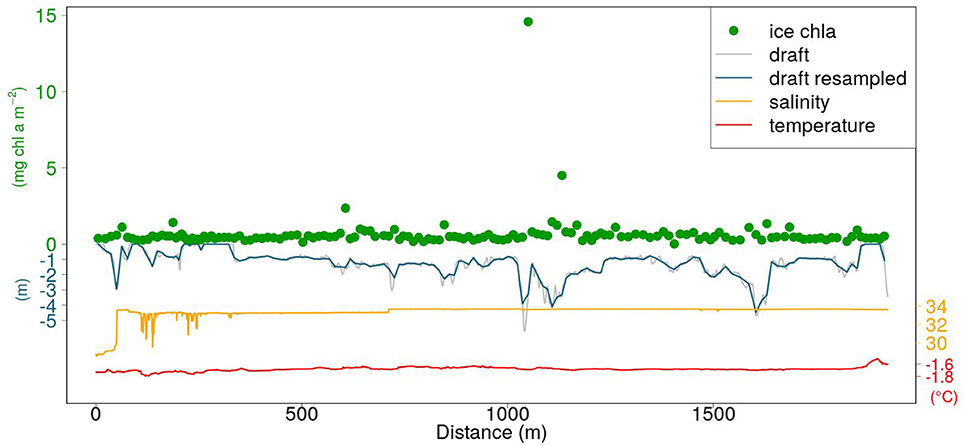
Figure 4. Example of a SUIT profile (station PS92-47_1). Orange and red lines represent surface salinity and temperature, respectively. The gray line is the draft obtained with Equation (1). The blue line is the draft resampled at the frequency of the RAMSES radiometers sampling (section 2.4). The green circles represent in-ice chl a retrieved by applying the NDI algorithm^c in Table 2.

2.5. Statistical Analysis

We applied Principal Component Analysis (PCA) to assess spatial and seasonal patterns in the variability of physical properties of the sea ice and the underlying water sampled by the SUIT separately for each hemisphere. We included in this analysis the parameters water temperature, salinity, total ice thickness from the present study, and ridge depth and ridge density (Rabenstein et al., 2010; Castellani et al., 2014, 2015, G. Castellani, unpublished data). Near-normal distribution of data, as assumed by PCA, was checked by visual inspection of histograms. In order to achieve near-normal distribution of the data, total ice thickness and ridge density were square-root transformed.

To test for significant differences between the frequency distributions of total ice thickness data from the EM-bird and the SUIT, we applied the Kolmogorov–Smirnov test. Before applying the test, the SUIT data were resampled to the footprint of the EM-bird (40 m) by averaging the data for each 40 m segment of each thickness profile. All statistical analyses were performed with the software R version 3.5.2 (R-Development-Core-Team, 2018), applying the package vegan (Oksanen et al., 2013).

2.6. Spatial Autocorrelation Analysis

Spatial autocorrelation was used to investigate the horizontal patchiness of sea-ice draft for 55 stations. Spatial autocorrelation analyses were also conducted for transmittance and in-ice chl a biomass. However, the transect nature of the surveys, the large interval spacing and small sample sizes, in comparison to draft, limited the spatial analyses of in-ice chl a to only 7 stations and of transmittance to only 10 stations. Autocorrelation was estimated using Moran's I (Moran, 1950; Legendre and Fortin, 1989; Legendre and Legendre, 1998), which was calculated for each SUIT survey at equally spaced (25 m) distance classes. Individual autocorrelation coefficients (e.g., Moran's I estimates) were plotted for each distance class as a spatial correlogram (Legendre and Fortin, 1989; Legendre and Legendre, 1998) using the R software function correlog from the pgirmess package (Giraudoux, 2018). Autocorrelation coefficients for each distance class were assigned a two-sided p-value according to Legendre and Fortin (1989) and Legendre and Legendre (1998). The presence of spatial autocorrelation (i.e., patchiness) was determined if the correlogram was considered globally significant at p < 0.05. We used the first x-intercept of globally significant correlogram lines as an indicator of the patch size for sea ice draft, Pd (Legendre and Fortin, 1989; Legendre and Legendre, 1998). This methodology is consistent with spatial autocorrelation analyses conducted on ROV gridded data from one of the same cruises (PS80, Lange et al., 2017b) and in other snow and sea ice studies (e.g., Gosselin et al., 1986; Rysgaard et al., 2001; Granskog et al., 2005; Søgaard et al., 2010).

3. Results

3.1. Arctic Ocean

3.1.1. Sea Ice and Under-Ice Water Properties

Under-ice water properties for the three Arctic expeditions are presented in detail in Tables 3–5. In spring (PS92 and PS106), under-ice water temperatures were lower and salinities were higher compared to summer (PS80). The mean under-ice water chl a was highest in spring (6.34 ± 5.94 mg m⁻² in May 2015, PS92) and lowest in autumn (1.60 ± 0.64 mg m⁻² in September 2012, PS80). Besides seasonal differences, the data also show a regional pattern. During spring 2015 (PS92) there was a distinct difference between Yermak stations and the stations on the Sophia Basin & shelf (Table 3). The latter had higher under-ice water chl a (with a mean of 12.52 ± 9.14 mg m⁻² compared to 1.80 ± 2.2 mg m⁻² for the Yermak stations), higher mean under-ice water temperature (−1.54 ± 0.13 °C compared to −1.77 ± 0.05 °C) and lower mean salinity (33.70 ± 0.43 compared to 34.13 ± 0.23). We could not confirm if this pattern was repeated on PS106 because the Yermak Plateau was not reached. However, during this expedition higher temperatures, lower salinities and very high chl a values (up to 20 mg m⁻²) in the surface layer were associated with the shelf-slope area toward the end of the expedition, and were probably related to the beginning of ice breakup (Table 4). During spring 2017 (PS106), time progression corresponded to a decrease in temperature and salinity and an increase in under-ice water chl a (PS106, Table 4). During summer 2012 (PS80), the stations situated in the Nansen Basin were characterized by higher salinities (mean 31.85 ± 0.94) and lower surface chl a (mean 0.66 ± 0.28 mg m⁻²), whereas stations in the Amundsen Basin had lower mean salinities (31.02 ± 1.71) and higher mean chl a concentrations (1.46 ± 0.60 mg m⁻², Table 5, David et al., 2015).

TABLE 3

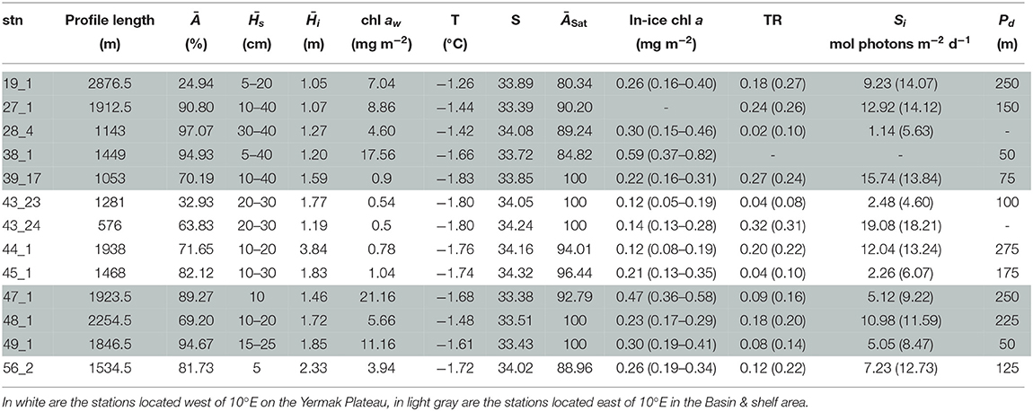
Table 3. Table for PS92 with, for each station (stn), the total profile length, the mean ice concentration (Ā) along profile, mean snow depth ($\overline{H_s}$) and mean total ice thickness ($\overline{H_i}$), under-ice water chl a (chl a_w) multiplied by the vertical section of the SUIT (2 m) to obtain integrated values, under-ice water temperature and salinity, ice concentration retrieved from satellite (Ā_Sat), median in-ice chl a (interquartile range), mean transmittance TR (± one standard deviation), mean Insolation S_i (± one standard deviation), and the draft patch size (P_d).

TABLE 4

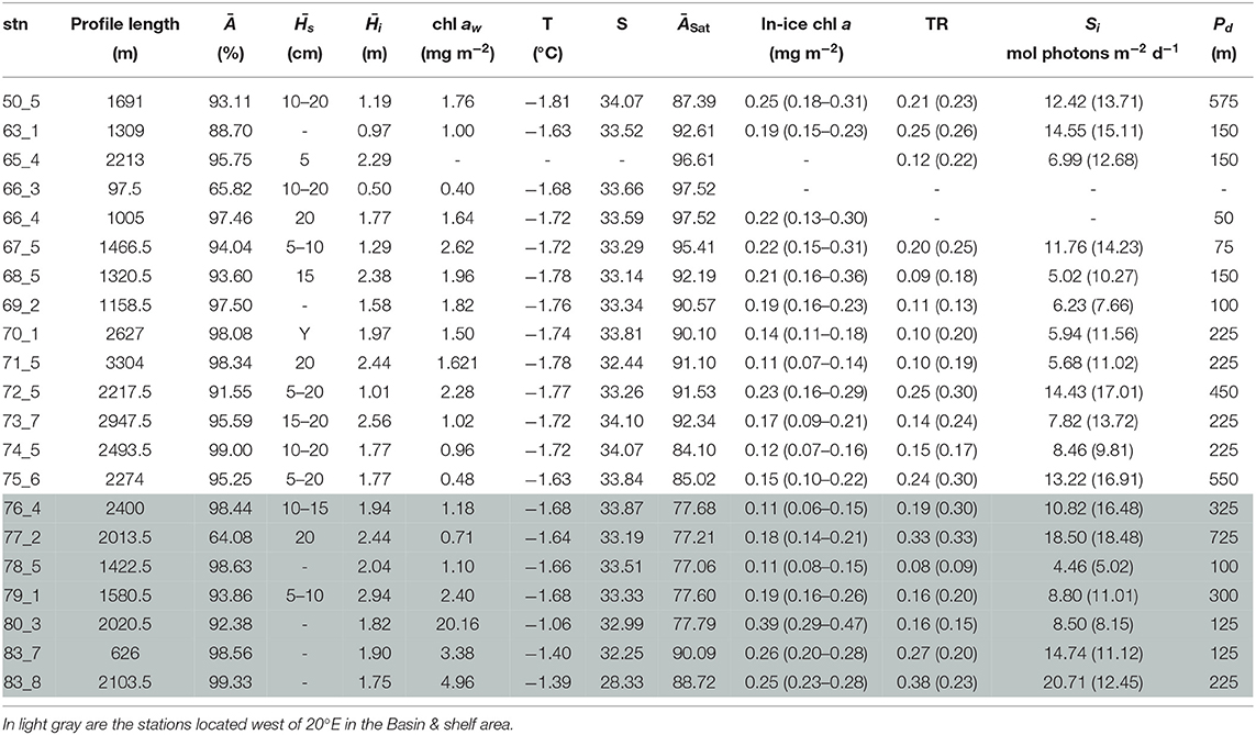
Table 4. Table for PS106 with, for each station (stn), the total profile length, the mean ice concentration (Ā) along profile, mean snow depth ($\overline{H_s}$) and mean total ice thickness ($\overline{H_i}$), under-ice water chl a (chl a_w) multiplied by the vertical section of the SUIT (2 m) to obtain integrated values, under-ice water temperature and salinity, ice concentration retrieved from satellite (Ā_Sat), and median in-ice chl a (interquartile range), mean transmittance TR (± one standard deviation), mean Insolation S_i (± one standard deviation), and the draft patch size (P_d).

TABLE 5

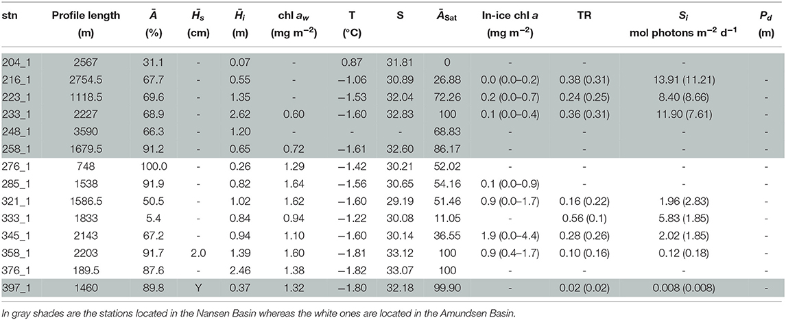
Table 5. Table for PS80 with, for each station (stn), the total profile length, the mean ice concentration (Ā) along profile, mean snow depth ($\overline{H_s}$) and mean total ice thickness ($\overline{H_i}$), under-ice water chl a (chl a_w) multiplied by the vertical section of the SUIT (2 m) to obtain integrated values, under-ice water temperature and salinity, ice concentration retrieved from satellite (Ā_Sat), and median in-ice chl a (interquartile range), mean transmittance TR (± one standard deviation), mean Insolation S_i (± one standard deviation), and the draft patch size (P_d).

During the springtime campaigns in 2015 (PS92) and 2017 (PS106), Arctic sea ice was covered with snow, whereas during summer 2012 (PS80) the ice surface was covered by melt ponds. Despite the difference in timing, snow depth decreased during both PS92 and PS106 and melt ponds started to form at the end of both expeditions (Tables 3, 4). Toward the end of summer 2012 (PS80), refreeze started and snow accumulated over the ice (Table 5). Modal sea-ice thickness (Figure 5) was the highest in the Arctic spring, with modes of 1.25 m and 1.65 m in 2015 (PS92) and 2017 (PS106), respectively, and lowest during the summer campaign in 2012 (PS80), with a primary mode for very thin ice (<10 cm). With an explained variability of 81.9% for the first two principal components, the outcome of the PCA (Figure 6A) confirms a high similarity of the two springtime data sets (PS92, PS106), and a distinctly different combination of physical sea-ice and under-ice properties in most stations sampled during summertime (PS80). Salinity and ridge properties were the main drivers of the variability in sea-ice and under-ice properties (Figure 6A). The analysis of regional patterns shows that total ice thickness decreased eastwards with a decrease of modal thickness from the Yermak stations (1.25 m) to the Sophia Basin & shelf stations (1.05 m) in May-June 2015 (PS92), and in July 2017 (PS106) from the Sophia Basin & shelf stations (1.75 m) to the stations east of 20°E (1.55 m).

FIGURE 5

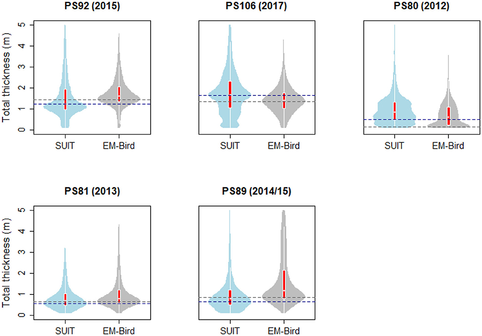
Figure 5. Violin plots of total thickness (sea ice and snow) computed from the SUIT stations and from the EM-bird measurements in the vicinity of SUIT stations. The “violins” show density functions of the relative frequency distribution of the data. Superimposed on the violin plots are box plots showing the median (white dot), the 1st to 3rd quartile range (red boxes), and the lowest and highest data points within approximate 1.5 times the interquartile range (white lines extending from the boxes). Dashed lines indicate the modes of SUIT (blue) and EM-Bird (gray) data. Data were restricted to the interval 0.1–5.0 m total thickness.

FIGURE 6

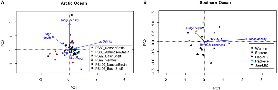
Figure 6. Principal component analysis for the Arctic Ocean and the Southern Ocean. In the Arctic Ocean (A), stations are divided within each expedition between Nansen and Amundsen basin (PS80), Yermak and Basin & shelf stations (PS92), and Basin & shelf stations vs. Western stations in the Nansen Basin (PS106). In the Southern Ocean (B), stations are divided between westernmost and eastermost stations (PS81), and between January MIZ, December MIZ, and pack-ice stations (PS89).

EM-bird data (Figure 5) show a similar pattern as the SUIT data, with a decrease in mean total ice thickness between spring and summer from 1.8 and 1.44 m during spring 2015 (PS92) and 2017 (PS106), respectively, to 0.71 m in summer 2012 (PS80). The shape of the ice-thickness distributions in spring was broadly similar between EM-bird data and SUIT data. However, a statistical comparison of the two data sets indicated significant differences between the two methods in all three sampling seasons (Kolmogorov–Smirnov test, p ≪ 0.001), probably due to differences of several decimeters in the modes of the thickness distributions. Histograms of total thickness for both the SUIT and the EM-bird data are presented in the Supplementary Material.

3.1.2. Under-Ice Light and Light-Derived In-Ice Chlorophyll a Concentration

Values of transmittance show a mode for TR < 0.05 in both spring and summer. However, the summer mean value is larger (0.203 compared to 0.136 and 0.184 in 2015 and 2017, respectively). During summer 2012, high transmittance values were more frequent compared to spring 2015 and 2017. The similarity in the distribution of transmittance data during spring 2015 and 2017, shows that the two campaigns sampled the same variability in sea-ice and snow conditions (Figure 7). A monthly comparison shows that there was a change in mean transmittance from 0.22 ± 0.03 in May 2015 to 0.33 ± 0.3 in August 2012, then a decrease to 0.12 ± 0.19 in September 2012. The extinction coefficient k_b calculated by non-linear regression from the May subset of the data showed the largest value with k_b = 8.678 m⁻¹. In June and July the extinction coefficients were lower, with values of 2.209 and 1.679 m⁻¹, respectively, reaching the minimum at 1.576 m⁻¹ in August (PS80). The extinction coefficient increased again in September to 6.552 m⁻¹. Insolation values in the Arctic (Figure 7) ranged from 0.00 to 57.17 mol photons m⁻² d⁻¹ during spring 2017 (PS106). In the comparison of May 2015 (PS92) and July (PS106), mean values ranged from 11.71 ± 14.17 mol photons m⁻² d⁻¹ to 10.24 ± 13.77 mol photons m⁻² d⁻¹, and maximum values from 45.12 to 57.17 mol photons m⁻² d⁻¹. During summer 2012, the shape of the distribution changed with respect to spring 2015 and 2017 and showed a smaller spread of values with maximum insolation at S_i = 36.35 mol photons m⁻² d⁻¹ compared to 51.77 mol photons m⁻² d⁻¹ and 57.17 mol photons m⁻² d⁻¹ during 2015 (PS92) and 2017 (PS106), respectively. Histograms of transmittance and insolation are presented in the Supplementary Material.

FIGURE 7

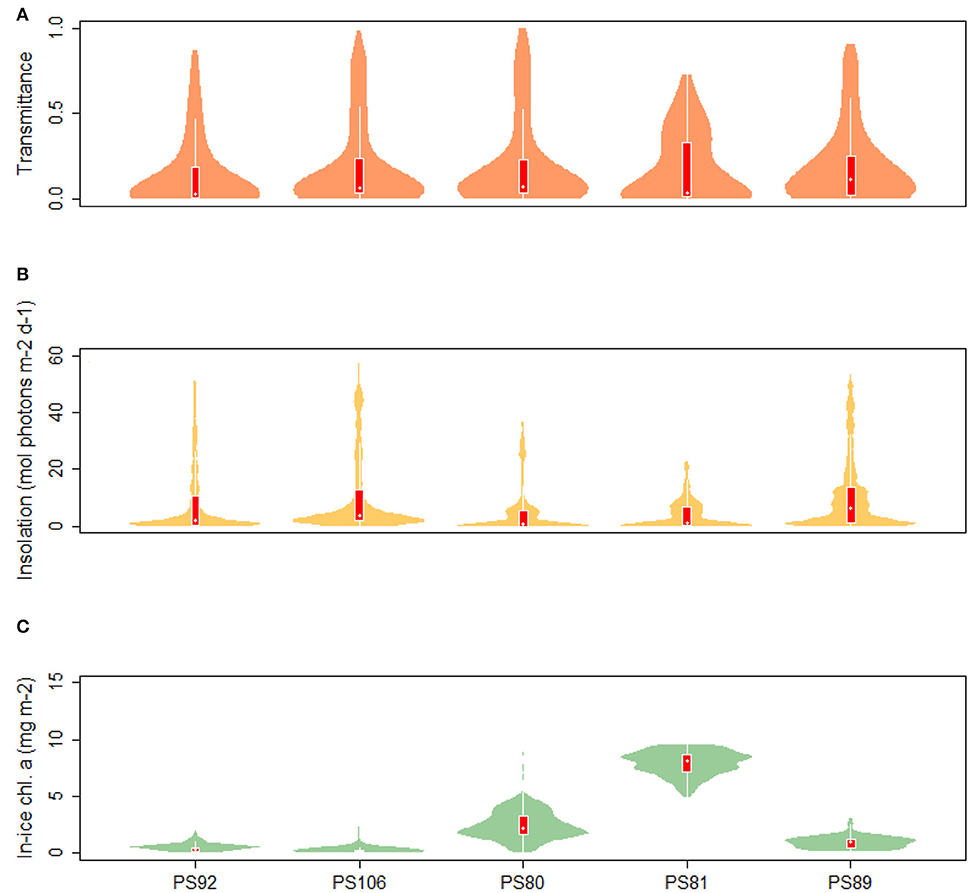
Figure 7. Violin plots of (A) transmittance, (B) insolation, and (C) chl a concentration in sea ice. The “violins” show density functions of the relative frequency distribution of the data. Superimposed on the violin plots are box plots showing the median (white dot), the 1st to 3rd quartile range (red boxes), and the lowest and highest data points within approximate 1.5 times the interquartile range (white lines extending from the boxes).

During PS92 the stations on the Yermak Plateau had the lowest in-ice chl a values, whereas the Basin & shelf stations had the highest (Table 3). High chl a concentrations were also found in the Basin & shelf area during PS106, but in this case the spatial variability was less pronounced (Table 4). During summer 2012 (PS80), the Nansen Basin presented lower values of in-ice chl a compared to the Amundsen Basin. In the area of overlap between PS80 and PS106 stations, chl a values from the two campaigns were very similar, varying around 0.2 mg chl a m⁻². Distributions of in-ice chl a are similar for the two spring campaigns, whereas the distribution of values from the summer campaign shows significantly higher values (Figure 7C). Histograms of in-ice chl a are presented in the Supplementary Material.

3.2. Antarctic

3.2.1. Sea Ice and Under-Ice Water Properties

During the Antarctic winter in 2013 (PS81), under-ice water temperatures were always close to the freezing point (Tables 1, 6) and uniform between sampling stations with a mean temperature of −1.85 ± 0.01°C. During summertime 2014/15 (PS89, Table 7), mean surface temperatures ranged between −1.67 ± 0.12 °C in the Dec-MIZ and −1.58 ± 0.12 °C in the Jan-MIZ. Lowest under-ice water temperatures characterized the pack-ice area sampled in December, with a mean of −1.86 ± 0.01°C. Likewise, the mean chl a concentration in the under-ice water was lower in winter 2013 (PS81, mean 0.42 ± 0.12 mg m⁻²) than in summer 2014/15 (PS89, mean 0.88 ± 0.62 mg m⁻²), and mean salinity was higher (34.22 ± 0.12 psu) in winter 2013 (PS81) than in summer 2014/15 (33.63 ± 0.24 psu). Between December (PS89, Dec-MIZ) and January (PS89, Jan-MIZ), both under-ice water temperature and chl a decreased, whereas salinity did not show any pattern (Table 7). The pack-ice area had different water properties compared to the MIZs, and it was characterized by significantly colder temperatures, more saline waters, and higher surface chl a concentrations (Table 7).

TABLE 6

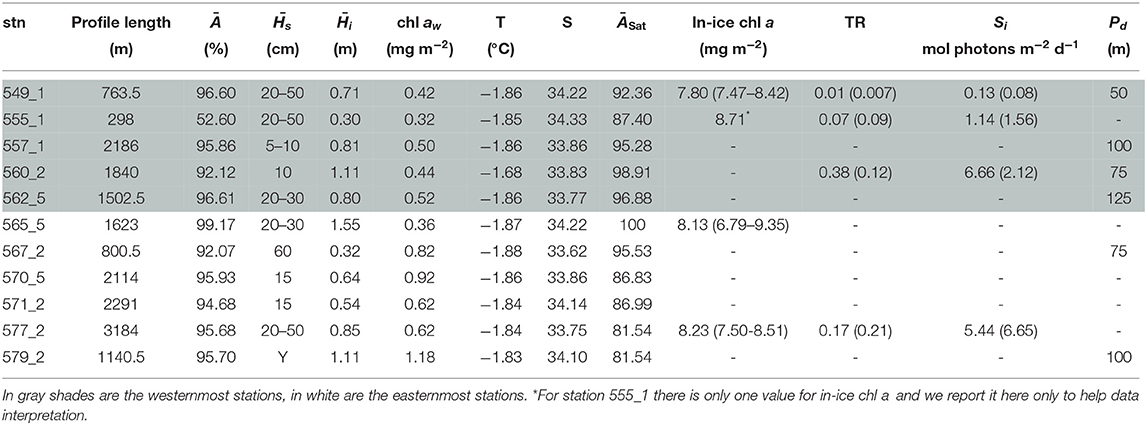
Table 6. Table for PS81 with, for each station (stn), the total profile length, the mean ice concentration (Ā) along profile, mean snow depth ($\overline{H_s}$) and mean total ice thickness ($\overline{H_i}$), under-ice water chl a (chl a_w) multiplied by the vertical section of the SUIT (2 m) to obtain integrated values, under-ice water temperature and salinity, ice concentration retrieved from satellite (Ā_Sat), and median in-ice chl a (interquartile range), mean transmittance TR (± one standard deviation), mean Insolation S_i (± one standard deviation), and the draft patch size (P_d).

TABLE 7

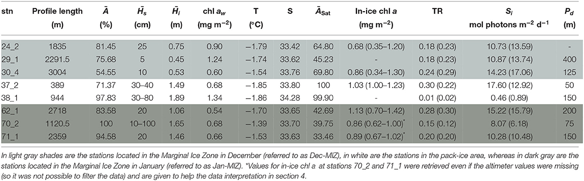
Table 7. Table for PS89 with, for each station (stn), the total profile length, the mean ice concentration (Ā) along profile, mean snow depth ($\overline{H_s}$) and mean total ice thickness ($\overline{H_i}$), under-ice water chl a (chl a_w) multiplied by the vertical section of the SUIT (2 m) to obtain integrated values, under-ice water temperature and salinity, ice concentration retrieved from satellite (Ā_Sat), and median in-ice chl a (interquartile range), mean transmittance TR (± one standard deviation), mean Insolation S_i (± one standard deviation), and the draft patch size (P_d).

Sea ice in the Southern Ocean was covered with snow during both winter 2013 (PS81, Table 6) and summer 2014/15 (PS89, Table 7). The snow depth ranged from 5 to 60 cm in winter 2013 (PS89) and from 5 and 100 cm in summer 2014/15 (PS89). Modal ice thickness was lowest in winter 2013 (PS81, 0.45 m) and highest in summer 2014/15 (PS89, 0.75 m) in the Jan-MIZ (Figure 5). During both expeditions, the differences in total ice thickness varied from thinner ice in the northern latitudes to thicker ice in southern parts of the sampling areas. In PS89, the shape of the thickness frequency distribution in the pack-ice zone was different from the ones of the MIZs with a longer tail toward larger thickness values (data not shown). Ice thickness distribution from the EM-bird data (Figure 5) was similar in shape to those of the SUIT for both expeditions. In EM-bird data, however, modal ice thicknesses were somewhat higher compared to SUIT data (Figure 5), with a mode of 0.65 m in winter (PS81), and a mode of 0.85 m in summer (PS89). As in the Arctic Ocean, a statistical comparison of the two data sets indicated significant differences between the two methods in both sampling seasons (Kolmogorov–Smirnov test, p < 0.001). Besides the differences in modal thickness, this difference was also related to greater variations in the sampling of very thin ice between the two methods, with a larger proportion of thinner ice in the SUIT data compared to EM-bird data.

The PCA biplot of the physical sea-ice and under-ice properties during the two Southern Ocean expeditions showed a gradual separation of the two sampling seasons, indicating that most stations sampled in winter (PS81) were associated with lower under-ice water temperatures and higher salinities than most stations sampled in summer (PS89) (Figure 6B). The cumulative explained variability of the two first principal components was 95.4%. Within each expedition, the PCA ordination reflected the differences between sampling regions (Figure 6B).

3.2.2. Under-Ice Light and Derived Chlorophyll a Concentration

In the Southern Ocean, distributions for transmittance show a principal mode at 0.05 during both winter 2013 (PS81) and summer 2014/15 (PS89) (Figure 7A). The spread of values was larger during summer, with a maximum transmittance of 0.91 in summer 2014 (PS89) compared to 0.73 in winter 2013 (PS81). A comparison between data from August (PS81) and January (PS89) did not show a significant difference in mean transmittance values, but a difference in maximum transmittance of 0.03 in August (PS81) and 0.9 in January (PS89). Extinction coefficients showed a large variability, with values ranging from k_b = 1.439 m⁻¹ in September 2013 (PS81) to k_b = 20.72 m⁻¹ in December 2014 (PS89). During both campaigns, insolation values showed a mode at S_i = 0.5 mol photons m⁻² d⁻¹, but mean values differed considerably with 3.86 ± 5.07 mol photons m⁻² d⁻¹ in winter 2013 (PS81) and 11.09 ± 13.08 in summer 2014/15 (PS89) (Figure 7B). The range of variability between winter and summer was very different, with a maximum at S_i = 22.72 mol photons m⁻² d⁻¹ in winter 2013 (PS81, Table 6) compared to S_i = 53.51 mol photons m⁻² d⁻¹ in December 2014 (PS89, Table 7).

During winter 2013, in-ice chl a was significantly higher than during summer, with a mean of 7.91 ± 1.07 mg chl a m⁻² in winter compared 0.88 ± 0.51 mg chl a m⁻² in summer (Figure 7C). Principal modes were at 8.5 and 1.3 mg chl a m⁻² during winter and summer, respectively. The variability within expeditions was low in both seasons. During summer 2014/15 higher in-ice chl a values were measured in the Jan-MIZ, compared to the Dec-MIZ.

3.3. Spatial Autocorrelation Analysis

The summary of the spatial autocorrelation analysis and the results for the patch size in both the Arctic and the Antarctic are presented in Table 8. Spatial autocorrelation analysis resulted in significant sea ice draft patch size estimates for 13 of the 19 SUIT stations in the Southern Ocean and 42 of the 48 SUIT stations in the Arctic Ocean, with significant results for almost all cruises. Patch size, which for ice draft can be interpreted as the size of smooth sea-ice areas, varied from 50 to 750 m with a mean of 221±156 m (Table 8) for the Arctic Ocean. In the Southern Ocean, autocorrelation analysis showed a draft patch size varying from 50 to 400 m (with an average of 129±92 m, Table 8), with larger values for the summer expedition (PS89). The spatial autocorrelation analysis for transmittance (i.e., patch sizes) showed statistical significant results for SUIT in 3 of the 19 SUIT stations in Antarctica and in 7 of the 48 SUIT stations in the Arctic Ocean, with no statistically significant results during the summer Arctic cruise PS80. Our analysis showed a significant Pearson's correlation between the patch size of draft and transmittance (correlation coefficient = 0.77; N = 9; p = 0.016), indicating that sea-ice draft (i.e., total ice thickness) is the driver of variability in sea-ice transmittance. Correlograms for one SUIT haul for each expedition are shown in Figure 8 together with a comparison in patch size between the two Polar regions for both ice draft and transmittance.

TABLE 8

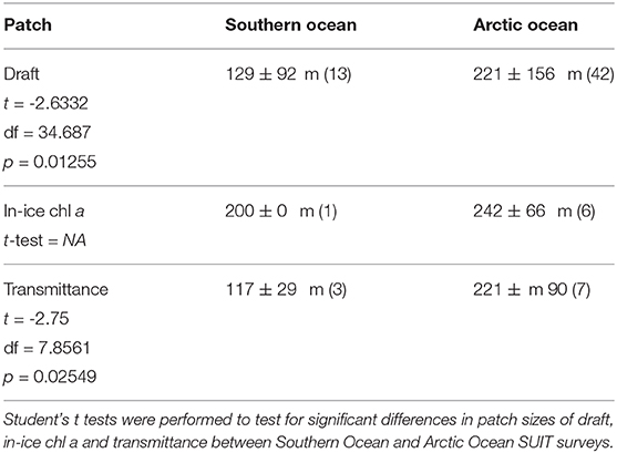
Table 8. Summary of the patch size for total thickness, transmittance and in-ice chl a as result of the spatial autocorrelation analysis (section 2.6).

FIGURE 8

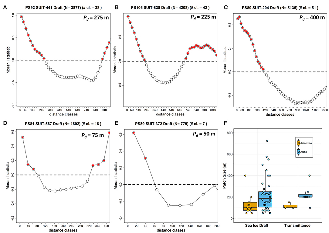
Figure 8. Correlograms showing Moran's I vs. distance classes for selected SUIT surveys as examples in the Arctic (top row): (A) PS80 station 204_1; (B) PS92 station 44_1; (C) PS106 station 83_8; and in Antarctica: (D) PS81 station 567_2; (E) PS89 station 37_2. Red filled circles represent significant values at p < 0.05. (F) Boxplot summarizing all sea ice draft patch sizes determined from all SUIT surveys grouped by polar region.

4. Discussion

4.1. Environmental Properties

This study presents the first characterization of sea ice and under-ice environments from multiple expeditions and seasons on the scale of kilometers in both ice-covered polar oceans. In the Arctic Ocean, ice and snow start to melt with the spring to summer progression and the increase in atmospheric and oceanic temperatures. The results showed this seasonal progression with a decrease of snow cover with subsequent formation of melt ponds, and a decrease of salinity in the under-ice water, an indicator of the presence of melt water under the ice. More light was found to penetrate the ice as time progressed, which can be attributed to a decrease in both ice thickness and snow cover (Tables 3–5). Similar patterns were seen in previous studies (e.g., Nicolaus et al., 2010). At some sampling stations, increased light penetration was accompanied by an increase of under-ice water chl a concentrations. During the two spring campaigns in 2015 and 2017 (PS92 and PS106), sampled locations were situated closely together with an overlap in the region 10°E < lon <20°E, defined as the Basin & shelf region. When comparing the two expeditions, the spatial pattern appeared stronger than the inter-annual one. During the PS92 expedition, the Basin & shelf region showed a difference in water masses, characterized by more saline and warmer water, compared to the Yermak Plateau (Meyer A. et al., 2017). The under-ice water chl a concentration was lower over the Yermak Plateau compared to the Basin & shelf region. In addition to these measurements, Assmy et al. (2017) found that the Basin & shelf area was characterized by large leads allowing light to penetrate through the ice which potentially explains increased chl a concentrations and a higher primary production compared to the Yermak region (Massicotte et al., 2019). The two regions also differed in the composition of under-ice fauna, and zooplankton abundances were generally very low in the under-ice water over the Yermak Plateau (Ehrlich et al., 2020). In summer 2012 (PS80), the Nansen vs. Amundsen Basin separation (Table 5) emerged clearly from the under-ice water salinity and chl a concentration, pointing to two different environmental regimes: an Atlantic influenced and nutrient-rich regime in the Nansen Basin, and a nutrient-poor regime influenced from the Laptev Sea shelf in the Amundsen Basin (David et al., 2015; Flores et al., 2019). Surface temperature, however, showed a seasonal decrease toward winter. Ice thickness differences between the two basins (not shown here) remained very small pointing to similar sea-ice conditions in the two basins (Figure 6A). However, the Amundsen Basin, which was sampled later in the season, had a principal mode at a thickness value of 0.65 m (figures not shown) and a secondary mode for very thin ice (values <0.1), indicating that refreeze started already. Additionally, under-ice water parameters differed between the two basins (Table 5), as well as the zooplankton community structure, which showed a dominance of copepods in the Nansen Basin, but a co-dominance of copepods and amphipods in the Amundsen Basin (David et al., 2015).

The shape of the total sea-ice thickness distributions from the SUIT data agreed largely with those from the EM-measurements. In both, the Arctic Ocean and the Southern Ocean, however, median and modal total thicknesses from the EM-bird and the SUIT differed by up to several decimeters, causing significant differences between the two distributions with no systematic bias toward one instrument (Figure 5). These differences could be due to differences in the geographical area covered by the two devices, thus one of the instruments might have collected a larger amount of data points in a region with thicker/thinner ice compared to the other instrument. This was particularly the case in PS89, where the EM-measurements included areas covered by landfast ice, which were not sampled with the SUIT (data not shown). Differences between SUIT and EM-measurements were probably also a result of a balance between systematic biases of the two devices: On the one hand, SUIT-based total thickness estimates could have been negatively biased because the ship tends to travel in areas where navigation is easier (i.e., thinner ice; PS92, PS81, PS89). On the other hand, the lower spatial resolution of the EM-measurements causes an under-representation of deep ridges compared to the SUIT, shifting the distribution of total thicknesses toward the lower end (PS106, PS80). Moreover, the way snow is treated might introduce bias. The EM-bird directly measures snow plus ice thickness, on the other hand, for the SUIT, ice draft is converted into total ice thickness. Therefore, a change in the actual snow depth will have different impacts on SUIT and EM-bird ice thickness retrievals. When comparing with satellite data (column Ā_Sat in Tables 3–7), the SUIT can provide representative ice-concentration values. Only in the marginal ice zone, where the SUIT preferentially sampled only the ice-covered parts of the grid cell detected by satellites, greater differences occurred (David et al., 2015).

Transmittance values largely reflected sea ice and snow conditions. The greater ice thickness during spring 2017 (PS106) compared to 2015 (PS92) was associated with lower mean transmittance values (Tables 3, 4), whereas the absence of snow during summer 2012 (PS80) led to higher transmittance (Table 5 and Figure 7). A larger spread of values during spring 2017 (PS106) compared to spring 2015 (PS92), however, points to higher variability of sea-ice and snow conditions, which was confirmed by Katlein et al. (2019), and which could be explained by the slightly different sampling period extending more toward summer during PS106. We estimated the insolation parameter (i.e., the daily integrated sunlight received) in order to obtain a representative comparison between SUIT hauls even if they were carried out at different times of the day. Mean insolation values in summer were higher than in spring, as a result of the larger transmittance values. However, the spread of values was wider in spring, which was related to incoming solar radiation that is maximum in the months of June-July compared to August-September (Arrigo et al., 2012; Arndt and Nicolaus, 2014). Extinction coefficients calculated from the present data set include the effect of both snow thickness and ice thickness, thus they represent bulk coefficients. Our summer values correspond to the ones generally known for bare ice (Grenfell and Maykut, 1977; Perovich, 1996; Light et al., 2008). The values presented here are in good agreement with those shown recently by Katlein et al. (2019), where bulk coefficients varied from ~5 m⁻¹ in May to ~1 m⁻¹ in August, and then increased again in September (Katlein et al., 2019, their Figure 8).

In the Southern Ocean, variations within winter 2013 (PS81) stations in salinity and temperature were rather small due to a quasi-homogeneous winter layer circulation in the Weddell Sea (David et al., 2017). The north-eastward sampling performed during the winter-spring transition led to a gradual decrease in sea-ice coverage, higher under-ice insolation, and an increase of under-ice water chl a by the end of the expedition, indicating that the productive season commenced (David et al., 2017). As for the Arctic expeditions, disentangling spatial and temporal patterns is challenging. Despite this difficulty, we can conclude that larger thickness values in the Jan-MIZ can be explained by the more southern locations. Total ice thickness distribution for winter 2013 (PS81) and summer 2014/15 (PS89) were similar, indicating similar sea-ice conditions. The cyclonic drift pattern of the Weddell Gyre moves sea ice from the eastern Weddell Sea/Lazarev Sea northwestward (Kwok et al., 2017) in a regime of mainly free drift. This decreases the tendency of sea ice to deform (G. Castellani, unpublished data) and it leads to more uniform sea-ice conditions in that area.

The similarity in snow cover and ice thickness between winter 2013 (PS81) and summer 2014/15 (PS89) leads to comparable transmittance values, even though the maximum transmittance values were lower in winter than in summer. Differently from the Arctic, Antarctic sea ice remained covered by relatively thick snow also during summer, explaining why transmittance values never approached 1.

4.2. In-Ice Chl a

We applied NDI and EOF algorithms to retrieve in-ice chl a from under-ice irradiance and transmittance spectra. We used one algorithm for Arctic summer (Lange et al., 2016), one for the Antarctic regions (Melbourne-Thomas et al., 2015), and one for the Arctic spring. In all the three cases, the retrieved values of in-ice chl a were in good agreement with ice-cores data collected during PS80 (Fernández-Méndez et al., 2015), and during PS92 and PS106 (Ehrlich et al., 2020, I. Peeken, unpublished data), and with derived in-ice chl a based on ROV measurements during PS81 (Meiners et al., 2017).

In the Arctic, the progression in snowmelt is visible in the increase of in-ice chl a with seasonal progression. Spring campaigns were conducted from late May onward, when incoming light levels were already high enough to cause an algal bloom, but snow cover obviously hampered this. Ice-algae growth was limited by the snow cover and the increase of in-ice chl a in the last stations during both PS92 and PS106 reflected the better light conditions after the onset of snowmelt. In-ice chl a concentrations were higher toward the end of summer 2012 (PS80) than in the two Arctic spring studies. This indicates that the ice-algae bloom only commenced after the onset of snowmelt, as expected from modeling studies (Castellani et al., 2017). During our sampling of PS80, large parts of the ice-algae bloom had already been released to the sea floor due to basal melting (Boetius et al., 2013), indicating that the observed in-ice chl a values had probably been considerably higher during the peak of the bloom.

In-ice chl a in the Antarctic winter was much higher than on any other expedition in the Arctic Ocean or the Southern Ocean. Our winter values agree well with values obtained from ice cores collected during the same expedition (Meiners et al., 2017). The presence of high biomass despite very low transmittance and insolation values indicate that the algae present in winter are the result of a previous accumulation of high biomass along the entire core length, more than an active growth at the bottom (Meiners et al., 2012). Winter in-ice algal assemblages often consist mainly of diatoms (Garrison and Close, 1993; Ugalde et al., 2016). During PS81 this was confirmed by sea-ice fatty acid compositions (Kohlbach et al., 2017b), and algae found in the stomach of larval krill (Schaafsma et al., 2017). Notably, in-ice chl a mean values in the Antarctic in winter were always higher than phytoplankton chl a values from the under-ice water. This was valid also for some stations during summer (i.e., stations 30_4, 37_2, 62_1, 70_1, and 71_1). Several Antarctic species are attracted to the sea ice during both summer and winter, including Antarctic krill Euphasia superba (Flores et al., 2011, 2012, 2014), showing the importance of sea ice-derived carbon for the Southern Ocean food web (Jia et al., 2016; Kohlbach et al., 2017b, 2018, 2019). This basal role of sea-ice derived carbon has a major impact on the distribution, abundance, life-cycle and possibly survival of many organisms residing in ice-covered oceans.

4.3. Physical and Biological Comparison

The present data set agrees with the well-known characteristics of the two polar regions, thus proves to be representative of the environment sampled. Variability in sea-ice properties was higher in the Arctic Ocean compared to the Southern Ocean. Furthermore, our spatial autocorrelation analysis of total sea-ice thickness showed smaller patch sizes in the Southern Ocean than in the Arctic Ocean. Interpreting this as bottom roughness, we can say that the Antarctic sea ice was characterized by smaller floes, or smaller patches of level ice compared to the Arctic, pointing to the different sea-ice drift, growth, and deformation regimes (Haas, 2008; Massom and Stammerjohn, 2010). Additionally, the correlation between total thickness and transmittance patch sizes indicates that, at floe-scales of around 120 m for the Southern Ocean and around 220 m for the Arctic Ocean, total ice thickness is a good predictor for transmittance, which is in agreement with previous work from the Arctic (e.g., Katlein et al., 2015). At smaller spatial scales, typically around 10 m, Katlein et al. (2015) found that surface properties such as melt ponds (during Arctic summer) were the best predictor for transmittance, which was not possible to resolve with the present data set due to the large spacing intervals between subsequent under-ice irradiance measurements (>10 m). The snow remains thick in the Antarctic during summer, whereas during Arctic summer snow melts completely and melt ponds form on the sea ice surface (Eicken, 2003; Nicolaus et al., 2012; Webster et al., 2018). Despite higher transmittance, insolation values (i.e., the amount of daily light that an algae receives at the bottom of the sea ice) were higher in the Arctic spring than in summer. The range of transmittance values during PS80 was higher compared to values collected in the same Arctic region and in the same season, but one year earlier, with a Remotely Operated Vehicle (ROV, Nicolaus and Katlein, 2013) diving under the ice (Nicolaus et al., 2012), and compared to those collected in July 2014 with an AUV diving under an ice floe (Katlein et al., 2015). The same holds for the transmittance values for PS81 and PS89: the range of transmittance variability measured with the SUIT was higher, and with higher mean values, than those obtained during the same expeditions with the ROV (PS81 data were published in Arndt et al., 2017, PS89 are unpublished data). Differences arise mainly from sampling methodologies. Whereas, with the ROV data are collected under a single, relatively uniform ice floe, the SUIT travels through a more heterogeneous environment, including also very thin ice or brash ice present in between ice floes. For this reason, the different methods sample differently and transmittance values can be higher when calculated from the SUIT data set compared to the ROV data set (Massicotte et al., 2019). Furthermore, a towed approach such as the SUIT is more robust compared to robotic platforms (e.g., ROVs and AUVs) and is thus able to ride directly along the underside of the sea ice at large distances with minimal concern about damage and losing the platform. However, the towed SUIT is subject to minimum speed requirements in order to maintain momentum while breaking sea ice and to representatively catch under-ice fauna, which is a main objective of SUIT deployments. Thus, ROVs and AUVs can survey the under ice environment at a more controlled and lower speed providing a greater spatial resolution, however, at the cost of spatial coverage.

As expected, insolation values were very low in winter (PS81). Despite the highest snow cover and the low transmittance values, during the Antarctic summer (PS89) the under-ice insolation was greater than in the Arctic summer (PS80). This difference reflected the different latitudinal ranges of the two sampling areas. The difference in maximum latitude (70°S compared to 85°N) and the difference in solar inclination lead to stronger incoming radiation during the Antarctic summer (PS89) than during the Arctic summer (PS80), leading to stronger under-ice insolation. Surface chl a values were higher in the Arctic (particularly in spring) than in the Antarctic. In contrast, in-ice chl a values were higher in Antarctic sea ice. Moreover, in the Arctic the amount of in-ice chl a was always lower than phytoplankton chl a, whereas the opposite is true in the Southern Ocean. This highlights the importance of sea ice-derived carbon especially for Antarctic ecosystems, both in summer and in winter.

Sea-ice represents a permanent or seasonal habitat for many species in the polar oceans. The SUIT does not only uniquely cover relatively large areas, but also enables a simultaneous sampling of environmental data and under-ice fauna (collected with the two nets attached to the SUIT frame). Collected data have, therefore, enabled the study of the relationship between the sea-ice environment and the distribution of zooplankton and nekton species at the ice-water interface at a scale of kilometers. The surface zooplankton communities of both the Arctic and Southern Ocean have been found to respond to the presence (or absence) of sea ice in all sampled seasons, and variations in under-ice zooplankton community structure have been related to sea-ice environmental properties (Flores et al., 2011, 2012, 2014, 2019; David et al., 2015, 2016; Schaafsma et al., 2017; Ehrlich et al., 2020). In the Arctic Ocean, for example, abrupt changes were observed from a dominance of ice-associated amphipods (Apherusa glacialis) at ice-covered stations to a dominance of pelagic amphipods (Themisto libellula) at nearby ice-free stations (David et al., 2015). In addition, high numbers of the copepods Calanus hyperboreus and Calanus glacialis were found in the ice-water interface layer, in spite of low under-ice water chl a within the sampling area (David et al., 2015), which indicated that they were grazing on ice algae (Runge and Ingram, 1991; Kohlbach et al., 2016). Higher abundances of the polar cod (Boreogadus saida), which is regarded as a key species in the Arctic Ocean, were related to relatively low under-ice surface salinity, thick sea-ice and high sea-ice coverage (David et al., 2016). In the Southern Ocean, differences in sea-ice drift pathways were closely related to the condition of krill larvae and the proportion of ice algae in their diet, at the beginning of the productive season (PS81) in the Weddell Sea (Kohlbach et al., 2017b; Schaafsma et al., 2017). The community structure of under-ice fauna was associated to changes in under-ice water parameters (David et al., 2017).

The presented data set and the environmental information from this study allow for further research on the relationship between large scale distributional patterns of under-ice fauna and sea-ice structures, such as the abundance and size of pressure ridges and hummocks, which have been suggested as structures where organisms, including both algae and zooplankton, accumulate (Gradinger et al., 2010; Lange et al., 2017a,b). Studies of Gradinger (1999) and Nozais et al. (2001) analyzed the potential role of sympagic fauna in controlling algal production due to grazing, but both drew contradictory conclusions. Whereas, Nozais et al. (2001) strongly suggest that the grazing impact of sea-ice meiofauna on ice algae was negligible, Gradinger (1999) found significant positive correlations between the integrated ice-algae and sympagic fauna biomass, and potential ingestion rates. Also other studies, often using data collected by divers, found evidence that abundance and distribution of certain species were related to the structure of the sea ice (Gruzov et al., 1967; Carey, 1985; Grainger and Hsiao, 1990; Garrison, 2015; Meyer B. et al., 2017), examples being the amphipods Gammarus wilkitzkii (Beuchel and Lønne, 2002) and Apherusa glaciali (Poltermann, 1998; Gradinger et al., 2010) in the Arctic Ocean. Gaining knowledge on the relationship between structure and faunal biomass on a larger scale, potentially will allow for prediction of an oceanwide distribution based on sea-ice parameters.

5. Conclusions

In this study, we presented and analyzed a large data set collected during five expeditions covering different years, seasons, and regions in both the Arctic Ocean and the Southern Ocean. Data were collected with a Surface and Under-Ice Trawl (SUIT), which allows the characterization of the sympagic environment on the kilometer scale. The data proved to be representative in characterizing the physical environment, and highlighted regional and seasonal differences in both hemispheres. Analysis of spatial variability showed a significant difference in the spatial scale of the variability of sea-ice properties between the Arctic and Antarctic, and showed that the total ice thickness was a driver for variability in sea-ice transmittance. The introduction of a new parameter, the insolation (i.e., daily integrated under-ice PAR) showed that more light for photosynthesis is available for biological production in the Antarctic summer compared to the Arctic summer, despite the large snow cover in the Antarctic and the higher transmittance in the Arctic. For the first time, we could provide in-ice chl a estimates over large spatial scales derived with the same methodology, for both the Arctic and the Antarctic. Our results showed that ice algae biomass was generally at comparable levels in both hemispheres during summertime, it was low in Arctic spring and particularly high in the Antarctic winter. In a future study, the present data set will be used to compare results and to improve parameters of sea-ice biogeochemical models.

Data Availability Statement

The datasets generated for this study are available at https://doi.pangaea.de/10.1594/PANGAEA.902056.

Author Contributions

GC wrote the paper, processed the data to obtain sea-ice draft and in-ice chl a, and prepared most of the figures. SA processed the RAMSES data to obtain integrated irradiance and radiance values and also to extract the wavelengths. RR provided the satellite ice concentration data. PM provided modeled downwelling irradiance data. IP supervised the Arctic sea ice biology sampling and processed all HPLC samples. FS, HF, and JE contributed to develop the structure of the manuscript and FS provided information on the snow depth per each SUIT haul. TK, SH, SS, and BL collected the EM-bird data. BL processed and plotted the EM-data, provided in-ice chl a estimates for PS80, and carried out the spatial autocorrelation analysis. GC, HF, JE, BL, FS, and CD contributed to SUIT data collection. JE, FS, CD, and HF contributed to data interpretation in connection with biological data. HF supervised the construction of the SUIT and designed the sampling for all the campaigns and conducted statistical analyses. All co-authors contributed to the discussion of results and to the preparation of the manuscript.

Funding

This study was primarily funded by the Helmholtz Association through the Young Investigators Group Iceflux (VH-NG-800) and the Research Program PACES II. RR was financed by the European Space Agency Climate Change Initiative Sea Ice project SK-ESA-2012-12. Antarctic research by Wageningen Marine Research is commissioned by the Netherlands Ministry of Agriculture, Nature and Food Quality (LNV) under its Statutory Research Task Nature & Environment WOT-04-009-047.04. The Netherlands Polar Programme (NPP), managed by the Netherlands Organisation for Scientific Research (NWO) funded this research under project nr. ALW 866.13.009. SA was financed by the German Research Council (DFG) in the framework of the priority programme Antarctic Research with comparative investigations in Arctic ice areas by grant to SPP1158, AR1236/1, and the Alfred-Wegener-Institut Helmholtz-Zentrum für Polar- und Meeresforschung. Part of this work resulted from the EcoLight project (grant number 03V01465), part of the Changing Arctic Ocean programme, jointly funded by the UK Natural Environment Research Council (NERC) and the German Federal Ministry of Education and Research (BMBF). JE was funded by the national scholarships “Promotionsstipendium nach dem Hamburger Nachwuchsfördergesetz (HmbNFG)” and “Gleichstellungsfond 2017 (4-GLF-2017)”, both granted by the University of Hamburg.

Conflict of Interest

The authors declare that the research was conducted in the absence of any commercial or financial relationships that could be construed as a potential conflict of interest.

Acknowledgments

We thank Captain Uwe Pahl, Captain Stefan Schwarze, Captain Thomas Wunderlich, and the crews of the RV Polarstern. We thank the scientific cruise leaders Antje Boetius (PS80), Bettina Meyer (PS81), Olaf Boebel (PS89), IP (PS92), and Andreas Macke and HF (PS106) for their excellent support and guidance with work at sea. We thank Jan Andries van Franeker (WUR) for kindly providing the Surface and Under-Ice Trawl (SUIT) and Michiel van Dorssen for technical support. The sampling with the SUIT, and on the ice, would have not been possible without the help of many volunteers during each expedition.

Supplementary Material

The Supplementary Material for this article can be found online at: https://www.frontiersin.org/articles/10.3389/fmars.2020.00536/full#supplementary-material

References

Arndt, S., Meiners, K. M., Ricker, R., Krumpen, T., Katlein, C., and Nicolaus, M. (2017). Influence of snow depth and surface flooding on light transmission through Antarctic pack ice. J. Geophys. Res. Oceans 122, 2108–2119. doi: 10.1002/2016JC012325

CrossRef Full Text | Google Scholar

Arndt, S., and Nicolaus, M. (2014). Seasonal cycle and long-term trend of solar energy fluxes through Arctic sea ice. Cryosphere 8, 2219–2233. doi: 10.5194/tc-8-2219-2014

CrossRef Full Text | Google Scholar

Arrigo, K. R. (2014). Sea ice ecosystems. Annu. Rev. Mar. Sci. 6, 439–467. doi: 10.1146/annurev-marine-010213-135103

CrossRef Full Text | Google Scholar

Arrigo, K. R., Perovich, D. K., Pickart, R. S., Brown, Z. W., van Dijken, G. L., Lowry, K. E., et al. (2012). Massive phytoplankton blooms under Arctic sea ice. Science 336, 1408–1408. doi: 10.1126/science.1215065

PubMed Abstract | CrossRef Full Text | Google Scholar

Assmy, P, Fernández-Méndez, M., Duarte, P, Meyer, A, Randelhoff, A, Mundy, C. J., et al. (2017). Leads in Arctic pack ice enable early phytoplankton blooms below snow-covered sea ice. Sci. Rep. 7:40850. doi: 10.1038/srep40850

PubMed Abstract | CrossRef Full Text | Google Scholar

Beuchel, F., and Lønne, O. (2002). Population dynamics of the sympagic amphipods Gammarus wilkitzkii and Apherusa glacialis in sea ice north of Svalbard. Polar Biol. 25, 241–250. doi: 10.1007/s00300-001-0329-8

CrossRef Full Text | Google Scholar

Boebel, O. (2015). The Expedition PS89 of the Research Vessel POLARSTERN to the Weddell Sea in 2014/2015. Berichte zur Polar- und Meeresforschung. Reports on Polar and Marine Research, 689.

Google Scholar

Boetius, A. (2013). The Expedition of the Research Vessel “Polarstern” to the Arctic in 2012 (ARK-XXVII/3). Berichte zur Polar- und Meeresforschung. Reports on Polar and Marine Research, 663.

Google Scholar

Boetius, A., Albrecht, S., Bakker, K., Bienhold, C., Felden, J., Fernández-Méndez, M., et al. (2013). Export of algal biomass from the melting Arctic sea ice. Science 339, 1430–1432. doi: 10.1126/science.1231346

PubMed Abstract | CrossRef Full Text | Google Scholar

Brierley, A., and Thomas, D. N. (2002). Ecology of southern ocean pack ice. Adv. Mar. Biol. 43, 171–276. doi: 10.1016/S0065-2881(02)43005-2

PubMed Abstract | CrossRef Full Text | Google Scholar

Budge, S. M., Wooller, M. J., Springer, A. M., Iverson, S. J., McRoy, C. P., and Divoky, G. J. (2008). Tracing carbon flow in an Arctic marine food web using fatty acid-stable isotope analysis. Oecologia 157, 117–129. doi: 10.1007/s00442-008-1053-7

PubMed Abstract | CrossRef Full Text | Google Scholar

Carey, A. (1985). “Marine ice fauna: arctic,” in Sea Ice Biota, ed. R. A. Horner (Boca Raton, FL: CRC Press), 173–190. doi: 10.1201/9781351076548-8

CrossRef Full Text | Google Scholar

Castellani, G., Gerdes, R., Losch, M., and Lüpkes, C. (2015). “Impact of sea-ice bottom topography on the Ekman pumping,” in Towards an Interdisciplinary Approach in Earth System Science, Springer Earth System Sciences, eds G. Lohmann, H. Meggers, V. Unnithan, D. Wolf-Gladrow, J. Notholt, and A. Bracher (Cham: Springer International Publishing), 139–148. doi: 10.1007/978-3-319-13865-7_16

CrossRef Full Text | Google Scholar

Castellani, G., Losch, M., Lange, B. A., and Flores, H. (2017). Modeling Arctic sea-ice algae: Physical drivers of spatial distribution and algae phenology. J. Geophys. Res. Oceans 122, 7466–7487. doi: 10.1002/2017JC012828

CrossRef Full Text | Google Scholar

Castellani, G., Lüpkes, C., Hendricks, S., and Gerdes, R. (2014). Variability of Arctic sea ice topography and its impact on the atmospheric surface drag. J. Geophys. Res. Oceans 119, 6743–6762. doi: 10.1002/2013JC009712

CrossRef Full Text | Google Scholar

David, C., Lange, B., Rabe, B., and Flores, H. (2015). Community structure of under-ice fauna in the Eurasian central Arctic Ocean in relation to environmental properties of sea-ice habitats. Mar. Ecol. Prog. Ser. 522, 15–32. doi: 10.3354/meps11156

CrossRef Full Text | Google Scholar

David, C., Lange, B. A., Krumpen, T., Schaafsma, F. L., van Franeker, J. A., and Flores, H. (2016). Under-ice distribution of polar cod Boreogadus saida in the central Arctic Ocean and their association with sea-ice habitat properties. Polar Biol. 39, 981–994. doi: 10.1007/s00300-015-1774-0

CrossRef Full Text | Google Scholar

David, C., Schaafsma, F. L., van Franeker, J. A., Lange, B. A., Brandt, A., and Flores, H. (2017). Community structure of under-ice fauna in relation to winter sea-ice habitat properties from the Weddell Sea. Polar Biol. 40, 247–261. doi: 10.1007/s00300-016-1948-4

CrossRef Full Text | Google Scholar

Dethloff, K., Handorf, D., Jaiser, R., Rinke, A., and Klinghammer, P. (2019). Dynamical mechanisms of Arctic amplification. Ann. N. Y. Acad. Sci. 1436, 184–194. doi: 10.1111/nyas.13698

PubMed Abstract | CrossRef Full Text | Google Scholar

Ehrlich, J., Schaafsma, F. L., Bluhm, B. A., Peeken, I., Castellani, G., Brandt, A., et al. (2020). Sympagic fauna in- and under arctic pack ice in the annual sea-ice system of the new arctic. Front. Mar. Sci. 7:452. doi: 10.3389/fmars.2020.00452

CrossRef Full Text | Google Scholar

Eicken, H. (1992). The role of sea ice in structuring Antarctic ecosystems. Polar Biol. 12, 3–13. doi: 10.1007/BF00239960

CrossRef Full Text | Google Scholar

Eicken, H. (2003). “Chapter 2: From the microscopic, to the macroscopic, to the regional scale: growth, microstructure and properties of sea ice,” in Sea Ice: An Introduction to its Physics, Chemistry, Biology and Geology, eds D. N. Thomas and G. S. Dieckmann (Blackwell Science Ltd.), 22–81. doi: 10.1002/9780470757161.ch2

CrossRef Full Text | Google Scholar

EUMETSAT (Ocean and Sea Ice Satellite Application Facility 2011). Ocean and Sea Ice Satellite Application Facility (2011), Global Sea Ice Concentration Reprocessing Dataset 1978-2009 (v1.1).

Google Scholar

Fernández-Méndez, M., Katlein, C., Rabe, B., Nicolaus, M., Peeken, I., Bakker, K., et al. (2015). Photosynthetic production in the central Arctic Ocean during the record sea-ice minimum in 2012. Biogeosciences 12, 3525–3549. doi: 10.5194/bg-12-3525-2015

CrossRef Full Text | Google Scholar

Ferrari, R., Jansen, M. F., Adkins, J. F., Burke, A., Stewart, A. L., and Thompson, A. F. (2014). Antarctic sea ice control on ocean circulation in present and glacial climates. Proc. Natl. Acad. Sci. U.S.A. 111, 8753–8758. doi: 10.1073/pnas.1323922111

PubMed Abstract | CrossRef Full Text | Google Scholar

Flores, H., David, C., Ehrlich, J., Hardge, K., Kohlbach, D., Lange, B. A., et al. (2019). Sea-ice properties and nutrient concentration as drivers of the taxonomic and trophic structure of high-Arctic protist and metazoan communities. Polar Biol. 42, 1377–1395. doi: 10.1007/s00300-019-02526-z

CrossRef Full Text | Google Scholar

Flores, H., Hunt, B. P., Kruse, S., Pakhomov, E. A., Siegel, V., van Franeker, J. A., et al. (2014). Seasonal changes in the vertical distribution and community structure of Antarctic macrozooplankton and micronekton. Deep Sea Res. I Oceanogr. Res. Pap. 84, 127–141. doi: 10.1016/j.dsr.2013.11.001

CrossRef Full Text | Google Scholar

Flores, H., van Franeker, J. A., Cisewski, B., Leach, H., Van de Putte, A. P., Meesters, E. H., et al. (2011). Macrofauna under sea ice and in the open surface layer of the Lazarev Sea, Southern Ocean. Deep Sea Res. II Top. Stud. Oceanogr. 58, 1948–1961. doi: 10.1016/j.dsr2.2011.01.010

PubMed Abstract | CrossRef Full Text | Google Scholar

Flores, H., van Franeker, J. A., Siegel, V., Haraldsson, M., Strass, V., Meesters, E. H., et al. (2012). The association of Antarctic krill Euphausia superba with the under-ice habitat. PLoS ONE 7:e31775. doi: 10.1371/journal.pone.0031775

PubMed Abstract | CrossRef Full Text | Google Scholar

Fofonoff, N. P. (1985). Physical properties of seawater: a new salinity scale and equation of state for seawater. J. Geophys. Res. Oceans 90, 3332–3342. doi: 10.1029/JC090iC02p03332

CrossRef Full Text | Google Scholar

Garrison, D., and Close, A. (1993). Winter ecology of the sea ice biota in Weddell Sea pack ice. Mar. Ecol. Prog. Ser. 96, 17–31. doi: 10.3354/meps096017

CrossRef Full Text | Google Scholar

Garrison, D. L. (2015). Antarctic sea ice biota. Integr. Comp. Biol. 31, 17–34. doi: 10.1093/icb/31.1.17

CrossRef Full Text | Google Scholar

Giraudoux, P. (2018). pgirmess: Spatial Analysis and Data Mining for Field Ecologists. R package version 1.6.9.

Google Scholar

Gosselin, M., Legendre, L., Therriault, J.-C., Demers, S., and Rochet, M. (1986). Physical control of the horizontal parchiness of sea-ice microalgae. Mar. Ecol. Prog. Ser. 29, 289–298. doi: 10.3354/meps029289

CrossRef Full Text | Google Scholar

Gradinger, R. (1999). Integrated abundance and biomass of sympagic meiofauna in Arctic and Antarctic pack ice. Polar Biol. 22, 169–177. doi: 10.1007/s003000050407

CrossRef Full Text | Google Scholar

Gradinger, R., Bluhm, B., and Iken, K. (2010). Arctic sea-ice ridges–Safe heavens for sea-ice fauna during periods of extreme ice melt? Deep Sea Res. II Top. Stud. Oceanogr. 57, 86–95. doi: 10.1016/j.dsr2.2009.08.008

CrossRef Full Text | Google Scholar

Grainger, E. H., and Hsiao, S. I. C. (1990). Trophic relationships of the sea ice meiofauna in Frobisher Bay, Arctic Canada. Polar Biol. 10, 283–292. doi: 10.1007/BF00238427

CrossRef Full Text | Google Scholar

Granskog, M., Kaartokallio, H., Kuosa, H., Thomas, D., Ehn, J., and Sonninen, E. (2005). Scales of horizontal patchiness in chlorophyll a, chemical and physical properties of landfast sea ice in the gulf of Finland (Baltic sea). Polar Biol. 28, 276–283. doi: 10.1007/s00300-004-0690-5

CrossRef Full Text | Google Scholar

Grenfell, T. C., and Maykut, G. A. (1977). The optical properties of ice and snow in the Arctic basin. J. Glaciol. 18, 445–463. doi: 10.1017/S0022143000021122

CrossRef Full Text | Google Scholar

Gruzov, Y., Propp, M., and Pushkin, A. (1967). Biological associations of coastal areas of the Davis Sea (based on the observations of divers). Sov. Antarct. Exped. Inf. Bull. 6, 523–533.

Google Scholar

Guerreiro, K., Fleury, S., Zakharova, E., Rémy, F., and Kouraev, A. (2016). Potential for estimation of snow depth on arctic sea ice from cryosat-2 and Saral/Altika missions. Remote Sens. Environ. 186, 339–349. doi: 10.1016/j.rse.2016.07.013

CrossRef Full Text | Google Scholar

Haas, C. (2008). “Chapter 3: Dynamics versus thermodynamics: the sea ice thickness distribution,” in Sea Ice: An Introduction to its Physics, Chemistry, Biology and Geology, eds D. N. Thomas and G. S. Dieckmann (John Wiley & Sons, Ltd.), 82–111. doi: 10.1002/9780470757161.ch3

CrossRef Full Text | Google Scholar

Haas, C., Lobach, J., Hendricks, S., Rabenstein, L., and Pfaffling, A. (2009). Helicopter-borne measurements of sea ice thickness, using a small and lightweight, digital EM system. J. Appl. Geophys. 67, 234–241. doi: 10.1016/j.jappgeo.2008.05.005

CrossRef Full Text | Google Scholar

Ivanova, N., Johannessen, O. M., Pedersen, L. T., and IEEE-Members Tonboe, R. T. (2014). Retrieval of arctic sea ice parameters by satellite passive microwave sensors: a comparison of eleven sea ice concentration algorithms. IEEE Trans. Geosci. Remote Sens. 52, 7233–7246. doi: 10.1109/TGRS.2014.2310136

CrossRef Full Text | Google Scholar

Jia, Z., Swadling, K. M., Meiners, K. M., Kawaguchi, S., and Virtue, P. (2016). The zooplankton food web under East Antarctic pack ice-A stable isotope study. Deep Sea Res. II Top. Stud. Oceanogr. 131, 189–202. doi: 10.1016/j.dsr2.2015.10.010

CrossRef Full Text | Google Scholar

Katlein, C., Arndt, S., Belter, H. J., Castellani, G., and Nicolaus, M. (2019). Seasonal evolution of light transmission distributions through Arctic sea ice. J. Geophys. Res. Oceans. 124, 5418–5435. doi: 10.1029/2018JC014833

CrossRef Full Text | Google Scholar

Katlein, C., Arndt, S., Nicolaus, M., Perovich, D. K., Jakuba, M. V., Suman, S., et al. (2015). Influence of ice thickness and surface properties on light transmission through Arctic sea ice. J. Geophys. Res. Oceans 120, 5932–5944. doi: 10.1002/2015JC010914

PubMed Abstract | CrossRef Full Text | Google Scholar

Katlein, C., Perovich, D. K., and Nicolaus, M. (2016). Geometric effects of an inhomogeneous sea ice cover on the under ice light field. Front. Earth Sci. 4:6. doi: 10.3389/feart.2016.00006

CrossRef Full Text | Google Scholar

Katlein, C., Schiller, M., Belter, H. J., Coppolaro, V., Wenslandt, D., and Nicolaus, M. (2017). A new remotely operated sensor platform for interdisciplinary observations under sea ice. Front. Mar. Sci. 4:281. doi: 10.3389/fmars.2017.00281

CrossRef Full Text | Google Scholar

Kohlbach, D., Graeve, M., Lange, B. A., David, C., Peeken, I., and Flores, H. (2016). The importance of ice algae-produced carbon in the central Arctic Ocean ecosystem: food web relationships revealed by lipid and stable isotope analyses. Limnol. Oceanogr. 61, 2027–2044. doi: 10.1002/lno.10351

PubMed Abstract | CrossRef Full Text | Google Scholar

Kohlbach, D., Graeve, M., Lange, B. A., David, C., Schaafsma, F. L., van Franeker, J. A., et al. (2018). Dependency of Antarctic zooplankton species on ice algae-produced carbon suggests a sea ice-driven pelagic ecosystem during winter. Glob. Change Biol. 24, 4667–4681. doi: 10.1111/gcb.14392

PubMed Abstract | CrossRef Full Text | Google Scholar

Kohlbach, D., Lange, B. A., Graeve, M., Vortkamp, M., and Flores, H. (2019). Varying dependency of Antarctic euphausiids on ice algae- and phytoplankton-derived carbon sources during summer. Mar. Biol. 166:79. doi: 10.1007/s00227-019-3527-z

CrossRef Full Text | Google Scholar

Kohlbach, D., Lange, B. A., Schaafsma, F. L., David, C., Vortkamp, M., Graeve, M., et al. (2017b). Ice algae-produced carbon is critical for overwintering of antarctic krill Euphausia superba. Front. Mar. Sci. 4:310. doi: 10.3389/fmars.2017.00310

PubMed Abstract | CrossRef Full Text | Google Scholar

Kohlbach, D., Schaafsma, F. L., Graeve, M., Lebreton, B., Lange, B. A., David, C., et al. (2017a). Strong linkage of polar cod (Boreogadus saida) to sea ice algae-produced carbon: evidence from stomach content, fatty acid and stable isotope analyses. Prog. Oceanogr. 152, 62–74. doi: 10.1016/j.pocean.2017.02.003

CrossRef Full Text | Google Scholar

Kwok, R., Pang, S. S., and Kacimi, S. (2017). Sea ice drift in the Southern Ocean: regional patterns, variability, and trends. Elem. Sci. Anth. 5:32. doi: 10.1525/elementa.226

CrossRef Full Text | Google Scholar

Laliberté, J., Bélanger, S., and Frouin, R. (2016). Evaluation of satellite-based algorithms to estimate photosynthetically available radiation (PAR) reaching the ocean surface at high northern latitudes. Remote Sens. Environ. 184, 199–211. doi: 10.1016/j.rse.2016.06.014

CrossRef Full Text | Google Scholar

Lange, B. A. (2017). Spatial variability of Arctic sea ice algae (Ph.D. thesis). University of Hamburg, Hamburg, Germany. Available online at: http://ediss.sub.uni-hamburg.de/volltexte/2017/8460

PubMed Abstract | Google Scholar

Lange, B. A., Beckers, J. F., Casey, J. A., and Haas, C. (2019). Airborne observations of summer thinning of multiyear sea ice originating from the Lincoln sea. J. Geophys. Res. Oceans 124, 243–266. doi: 10.1029/2018JC014383

PubMed Abstract | CrossRef Full Text | Google Scholar

Lange, B. A., Flores, H., Michel, C., Beckers, J. F., Bublitz, A., Casey, J. A., et al. (2017a). Pan-Arctic sea ice-algal chl a biomass and suitable habitat are largely underestimated for multiyear ice. Glob. Change Biol. 23, 4581–4597. doi: 10.1111/gcb.13742

PubMed Abstract | CrossRef Full Text | Google Scholar

Lange, B. A., Katlein, C., Castellani, G., Fernández-Méndez, M., Nicolaus, M., Peeken, I., et al. (2017b). Characterizing spatial variability of ice algal chlorophyll a and net primary production between sea ice habitats using horizontal profiling platforms. Front. Mar. Sci. 4:349. doi: 10.3389/fmars.2017.00349

CrossRef Full Text | Google Scholar

Lange, B. A., Katlein, C., Nicolaus, M., Peeken, I., and Flores, H. (2016). Sea ice algae chlorophyll a concentrations derived from under-ice spectral radiation profiling platforms. J. Geophys. Res. Oceans. 121, 8511–8534. doi: 10.1002/2016JC011991

CrossRef Full Text | Google Scholar

Legendre, L., and Gosselin, M. (1991). In situ spectroradiometric estimation of microalgal biomass in first-year sea ice. Polar Biol. 11, 113–115. doi: 10.1007/BF00234273

CrossRef Full Text | Google Scholar

Legendre, P., and Fortin, M. J. (1989). Spatial pattern and ecological analysis. Vegetatio 80, 107–138. doi: 10.1007/BF00048036

CrossRef Full Text | Google Scholar

Legendre, P., and Legendre, L. (1998). “Spatial analysis,” in Numerical Ecology, eds P. Legendre and L. Legendre (Amsterdam, BV: Elsevier Science), 707–786.

Google Scholar

Light, B., Grenfell, T. C., and Perovich, D. K. (2008). Transmission and absorption of solar radiation by Arctic sea ice during the melt season. J. Geophys. Res. Oceans 113:C03023. doi: 10.1029/2006JC003977

CrossRef Full Text | Google Scholar

Liu, Z. (2012). Dynamics of interdecadal climate variability: a historical perspective. J. Clim. 25, 1963–1995. doi: 10.1175/2011JCLI3980.1

CrossRef Full Text | Google Scholar

Macke, A., and Flores, H. (2018). The Expeditions PS106/1 and 2 of the Research Vessel POLARSTERN to the Arctic Ocean in 2017. Berichte zur Polar- und Meeresforschung. Reports on Polar and Marine Research, 719.

Google Scholar

Massicotte, P., Peeken, I., Katlein, C., Flores, H., Huot, Y., Castellani, G., et al. (2019). Sensitivity of phytoplankton primary production estimates to available irradiance under heterogeneous sea-ice conditions. J. Geophys. Res. Oceans. 124, 5436–5450. doi: 10.1029/2019JC015007

CrossRef Full Text | Google Scholar

Massom, R. A., and Stammerjohn, S. E. (2010). Antarctic sea ice change and variability-physical and ecological implications. Polar Sci. 4, 149–186. doi: 10.1016/j.polar.2010.05.001

CrossRef Full Text | Google Scholar

Maykut, G. A., and Grenfell, T. C. (1975). The spectral distribution of light beneath first-year sea ice in the Arctic Ocean. Limnol. Oceanogr. 20, 554–563. doi: 10.4319/lo.1975.20.4.0554

CrossRef Full Text | Google Scholar

McMinn, A., Pankowskii, A., Ashworth, C., Bhagooli, R., Ralph, P., and Ryan, K. (2010). In situ net primary productivity and photosynthesis of Antarctic sea ice algal, phytoplankton and benthic algal communities. Mar. Biol. 157, 1345–1356. doi: 10.1007/s00227-010-1414-8

CrossRef Full Text | Google Scholar

Meiners, K. M., Arndt, S., Bestley, S., Krumpen, T., Ricker, R., Milnes, M., et al. (2017). Antarctic pack ice algal distribution: Floe-scale spatial variability and predictability from physical parameters. Geophys. Res. Lett. 44, 7382–7390. 2017GL074346. doi: 10.1002/2017GL074346

CrossRef Full Text | Google Scholar

Meiners, K. M., Vancoppenolle, M., Thanassekos, S., Dieckmann, G. S., Thomas, D. N., Tison, J.-L., et al. (2012). Chlorophyll a in Antarctic sea ice from historical ice core data. Geophys. Res. Lett. 39:L21602. doi: 10.1029/2012GL053478

PubMed Abstract | CrossRef Full Text | Google Scholar

Melbourne-Thomas, J., Meiners, K. M., Mundy, C. J., Schallenberg, C., Tattersall, K. L., and Dieckmann, G. S. (2015). Algorithms to estimate Antarctic sea ice algal biomass from under-ice irradiance spectra at regional scales. Mar. Ecol. Prog. Ser. 536, 107–121. 10.3354/meps11396. doi: 10.3354/meps11396

CrossRef Full Text | Google Scholar

Meyer, A, Sundfjord, A., Fer, I., Provost, C., Villacieros Robineau, N., Koenig, Z., et al. (2017). Winter to summer oceanographic observations in the Arctic Ocean north of Svalbard. J. Geophys. Res. Oceans 122, 6218–6237. doi: 10.1002/2016JC012391

CrossRef Full Text | Google Scholar

Meyer, B, Freier, U, Grimm, V, Groeneveld, J, Hunt, B. P. V, and Kerwath, S. (2017). The winter pack-ice zone provides a sheltered but food-poor habitat for larval Antarctic krill. Nat. Ecol. Evol. 1, 1853–1861. doi: 10.1038/s41559-017-0368-3

PubMed Abstract | CrossRef Full Text | Google Scholar

Meyer, B., and Auerswald, L. (2014). The Expedition of the Research Vessel “Polarstern” to the Antarctic in 2013 (ANT-XXIX/7). Berichte zur Polar- und Meeresforschung. Reports on Polar and Marine Research, 674.

Google Scholar

Miller, L., Fripiat, F., Else, B., Bowman, J., Brown, K., Collins, R., et al. (2015). Methods for biogeochemical studies of sea ice: the state of the art, caveats, and recommendations. Elem. Sci. Anth. 3:000038. doi: 10.12952/journal.elementa.000038

CrossRef Full Text | Google Scholar

Moran, P. A. P. (1950). Notes on continuous stochastic phenomena. Biometrika 37, 17–23. doi: 10.1093/biomet/37.1-2.17

PubMed Abstract | CrossRef Full Text | Google Scholar

Mundy, C. J., Ehn, J. K., Barber, D. G., and Michel, C. (2007). Influence of snow cover and algae on the spectral dependence of transmitted irradiance through Arctic landfast first-year sea ice. J. Geophys. Res. Oceans 112:C03007. doi: 10.1029/2006JC003683

CrossRef Full Text | Google Scholar

Nicolaus, M., Gerland, S., Hudson, S. R., Hanson, S., Haapala, J., and Perovich, D. K. (2010). Seasonality of spectral albedo and transmittance as observed in the Arctic Transpolar Drift in 2007. J. Geophys. Res. Oceans 115:C11011. doi: 10.1029/2009JC006074

CrossRef Full Text | Google Scholar

Nicolaus, M., and Katlein, C. (2013). Mapping radiation transfer through sea ice using a remotely operated vehicle (ROV). Cryosphere 7, 763–777. doi: 10.5194/tc-7-763-2013

CrossRef Full Text | Google Scholar

Nicolaus, M., Katlein, C., Maslanik, J. A., and Hendricks, S. (2012). Changes in Arctic sea ice result in increasing light transmittance and absorption. Geophys. Res. Lett. 39, 2699–2700. doi: 10.1029/2012GL053738

CrossRef Full Text | Google Scholar

Nozais, C., Gosselin, M., Michel, C., and Tita, G. (2001). Abundance, biomass, composition and grazing impact of the sea-ice meiofauna in the North Water, northern Baffin Bay. Mar. Ecol. Prog. Ser. 217, 235–250. 10.3354/meps217235. doi: 10.3354/meps217235

CrossRef Full Text | Google Scholar

Oksanen, J., Blanchett, F., Kindt, R., Legendre, P., Minchin, P., O'Hara, R., et al. (2013). Vegan: Community Ecology Package Version 2.0-10.

Google Scholar

Peeken, I. (2016). The Expedition PS92 of the Research Vessel POLARSTERN to the Arctic Ocean in 2015. Berichte zur Polar- und Meeresforschung. Reports on Polar and Marine Research, 694.

Google Scholar

Perovich, D. K. (1990). Theoretical estimates of light reflection and transmission by spatially complex and temporally varying sea ice covers. J. Geophys. Res. Oceans 95, 9557–9567. doi: 10.1029/JC095iC06p09557

CrossRef Full Text | Google Scholar

Perovich, D. K. (1996). The optical properties of sea ice (Ph.D. thesis). U.S. Army Cold Regions Research and Engineering Laboratory, Hanover, NH, United States.

PubMed Abstract | Google Scholar

Poltermann, M. (1998). Abundance, biomass and small-scale distribution of cryopelagic amphipods in the Franz Josef Land area (Arctic). Polar Biol. 20, 134–138. doi: 10.1007/s003000050287

CrossRef Full Text | Google Scholar

Rabenstein, L., Hendricks, S., Martin, T., Pfaffhuber, A., and Haas, C. (2010). Thickness and surface-properties of different sea-ice regimes within the Arctic Trans Polar Drift: data from summers 2001, 2004 and 2007. J. Geophys. Res. 115:C12059. doi: 10.1029/2009JC005846

CrossRef Full Text | Google Scholar

R-Development-Core-Team (2018). R: A Language and Environment for Statistical Computing.

Google Scholar

Ricchiazzi, P., Yang, S., Gautier, C., and Sowle, D. (1998). SBDART: a research and teaching software tool for plane-parallel radiative transfer in the Earth's atmosphere. Bull. Am. Meteorol. Soc. 79, 2101–2114. doi: 10.1175/1520-0477(1998)079<2101:SARATS>2.0.CO;2

CrossRef Full Text | Google Scholar

Ricker, R., Hendricks, S., Perovich, D. K., Helm, V., and Gerdes, R. (2015). Impact of snow accumulation on CryoSat-2 range retrievals over Arctic sea ice: an observational approach with buoy data. Geophys. Res. Lett. 42, 4447–4455. doi: 10.1002/2015GL064081

CrossRef Full Text | Google Scholar

Runge, J. A., and Ingram, R. G. (1991). Under-ice feeding and diel migration by the planktonic copepods Calanus glacialis and Pseudocalanus minutus in relation to the ice algal production cycle in southeastern Hudson Bay, Canada. Mar. Biol. 108, 217–225. doi: 10.1007/BF01344336

CrossRef Full Text | Google Scholar

Rysgaard, S., Kuhl, M., Glud, R., and Hansen, J. (2001). Biomass, production and horizontal patchiness of sea ice algae in a high-arctic fjord (young sound, NE Greenland). Mar. Ecol. Prog. Ser. 223, 15–26. doi: 10.3354/meps223015

CrossRef Full Text | Google Scholar

Schaafsma, F., Kohlbach, D., David, C., Lange, B. A., Graeve, M., Flores, H., and van Franeker, J. A. (2017). Spatio-temporal variability in the winter diet of larval and juvenile Antarctic krill, Euphausia superba, in ice-covered waters. Mar. Ecol. Prog. Ser. 580, 101–115. doi: 10.3354/meps12309

CrossRef Full Text | Google Scholar

Schaafsma, F. L. (2018). Life in the polar oceans: the role of sea ice in the biology and ecology of marine species (Ph.D. thesis). Wageningen University, Wageningen, Netherlands.

Google Scholar

Schaafsma, F. L., David, C., Pakhomov, E. A., Hunt, B. P. V., Lange, B. A., Flores, H., et al. (2016). Size and stage composition of age class 0 Antarctic krill Euphausia superba in the ice-water interface layer during winter/early spring. Polar Biol. 39, 1515–1526. doi: 10.1007/s00300-015-1877-7

CrossRef Full Text | Google Scholar

Schmitz, W. J. Jr. (1995). On the interbasin-scale thermohaline circulation. Rev. Geophys. 33, 151–173. doi: 10.1029/95RG00879

CrossRef Full Text | Google Scholar

Søgaard, D., Kristensen, M., Rysgaard, S., Glud, R., Hansen, P., and Hilligsøe, K. (2010). Autotrophic and heterotrophic activity in arctic first-year sea ice: seasonal study from Malene Bight, SW Greenland. Mar. Ecol. Prog. Ser. 419, 31–45. doi: 10.3354/meps08845

CrossRef Full Text | Google Scholar

Søreide, J. E., Hop, H., Carroll, M. L., Falk-Petersen, S., and Hegseth, E. N. (2006). Seasonal food web structures and sympagic-pelagic coupling in the European arctic revealed by stable isotopes and a two-source food web model. Prog. Oceanogr. 71, 59–87. doi: 10.1016/j.pocean.2006.06.001

CrossRef Full Text | Google Scholar

Swadling, K. M., Gibson, J. A. E., Ritz, D. A., Nichols, P. D., and Hughes, D. E. (1997). Grazing of phytoplankton by copepods in eastern Antarctic coastal waters. Mar. Biol. 128, 39–48. doi: 10.1007/s002270050066

CrossRef Full Text | Google Scholar

Tran, S., Bonsang, B., Gros, V., Peeken, I., Sarda-Esteve, R., Bernhardt, A., et al. (2013). A survey of carbon monoxide and non-methane hydrocarbons in the Arctic Ocean during summer 2010. Biogeosciences 10, 1909–1935. doi: 10.5194/bg-10-1909-2013

CrossRef Full Text | Google Scholar

Ugalde, S. C., Westwood, K. J., van den Enden, R., McMinn, A., and Meiners, K. M. (2016). Characteristics and primary productivity of East Antarctic pack ice during the winter-spring transition. Deep Sea Res. II Top. Stud. Oceanogr. 131, 123–139. doi: 10.1016/j.dsr2.2015.12.013

CrossRef Full Text | Google Scholar

van Franeker, J. A., Flores, H., and van Dorssen, M. (2009). The surface and under ice trawl (SUIT) (Ph.D. thesis). University of Groningen, Groningen, Netherlands.

PubMed Abstract | Google Scholar

Wang, S. W., Budge, S. M., Iken, K., Gradinger, R., Springer, A. M., and Wooller, M. J. (2015). Importance of sympagic production to Bering Sea zooplankton as revealed from fatty acid-carbon stable isotope analyses. Mar. Ecol. Prog. Ser. 518, 31–50. doi: 10.3354/meps11076

CrossRef Full Text | Google Scholar

Wang, S. W., Springer, A. M., Budge, S. M., Horstmann, L., Quakenbush, L. T., and Wooller, M. J. (2016). Carbon sources and trophic relationships of ice seals during recent environmental shifts in the Bering Sea. Ecol. Appl. 26, 830–845. doi: 10.1890/14-2421

PubMed Abstract | CrossRef Full Text | Google Scholar

Webster, M, Gerland, S, Holland, M, Hunke, E, Kwok, R, and Lecomte, O. (2018). Snow in the changing sea-ice systems. Nat. Clim. Change 8, 946–953. doi: 10.1038/s41558-018-0286-7

CrossRef Full Text | Google Scholar

Wongpan, P., Meiners, K. M., Langhorne, P. J., Heil, P., Smith, I. J., Leonard, G. H., et al. (2018). Estimation of Antarctic land-fast sea ice algal biomass and snow thickness from under-ice radiance spectra in two contrasting areas. J. Geophys. Res. Oceans 123, 1907–1923. doi: 10.1002/2017JC013711

CrossRef Full Text | Google Scholar