Potential Consequences of Climate and Management Scenarios for the Northeast Atlantic Mackerel Fishery

Introduction

Mackerel (S. scombrus, NEAM) is among the most widely-distributed and economically valuable fish stocks in the Northeast Atlantic (Trenkel et al., 2014; Jansen et al., 2016). An increase in stock size over recent years has supported large catches, which reached a peak in 2014 at around 1.4 million tons (ICES, 2019c). As a result, the NEAM fishery is now a major contributor to the economies of several coastal states in the Northeast Atlantic (Jansen et al., 2016). Although current stock size is high, it is estimated that recent levels of exploitation will lead to sub-optimal yield in the long-term due to overfishing (ICES, 2019c). This in part because, despite agreeing on a management strategy in 2015, the European Union, Norway and the Faroe Islands have since all declared quotas above those advised by the International Council for the Exploration of the Seas (ICES) (ICES, 2019a). Management of NEAM is further complicated by the fact that the spatial distribution of the stock in the summer months has recently expanded (Berge et al., 2015; Ólafsdóttir et al., 2018). It is now found in substantial numbers in the jurisdictions of Iceland and Greenland which previously had no share of the catch (Kooij et al., 2015; Olafsdottir et al., 2016). Both countries have since set unilateral quotas without international agreement (ICES, 2019a). Given the commercial value of the NEAM stock it is crucial that the fishery is managed appropriately in order to preserve the economic benefits it currently provides.

Management of NEAM depends on scientific advice regarding acceptable levels of exploitation. This advice is provided by ICES, who assess the state of the stock using an age-structured state-space assessment model (SAM) (Nielsen and Berg, 2014). The first step in the stock assessment is to estimate current levels of spawning stock biomass (SSB) and the rate of fishing mortality (F). These outputs are then used as starting points for forecasts of future stock status under various catch scenarios, which inform the advisory total allowable catch (TAC) for the following year [see ICES (2019a) and earlier advice reports]. SAM is used in stock assessment because it is able to assimilate the large amounts of data required (e.g., catch, tag-recapture, survey indices), and can tractably estimate many parameters. However, like most models used for stock assessment (MacKenzie et al., 2008; Goethel et al., 2011; Kuparinen et al., 2012), SAM does not incorporate the spatial structure of a stock or any environmental influence on its population dynamics. For this reason, it is limited in its ability to make predictions about: (1) longer-term fluctuations in the stock which may be affected by changing climate; and (2) the effects of spatial management measures which depend on a stock’s distribution.

Spatial management in fisheries is becoming increasingly prevalent (Halpern et al., 2012), often in the form of seasonal or permanent area closures in which certain stocks may not be targeted (Hall, 2001; STECF, 2007). With respect to the NEAM fishery, sectors of the North Sea are subject to closures for different portions of the year. Mackerel fishing is not permitted in the southern and central regions of the North Sea at any time (ICES, 2019c). This measure was implemented to protect the North Sea spawning component of the NEAM stock, which has not recovered since being heavily depleted in the 1970s (Jansen, 2014). The Northern region of the North Sea is subject to a seasonal closure from February 15th to July 31st each year. The reason that mackerel fishing is permitted in the Northern North Sea outside of this period (August 1st to February 14th) is that the much larger western spawning component of the stock migrates into the area in large numbers during this time. ICES recommends that existing area closures remain in place to protect the North Sea spawning component (ICES, 2019c), but understanding the effects of closures is difficult. One approach that has been used to study the effects of spatial fishery management options is to implement them in spatially explicit models and test how the populations respond. For example, spatially explicit individual-based models (IBMs) have been used predict how fish communities may respond to the implementation of marine protected areas (Yemane et al., 2009; Brochier et al., 2013).

In addition to exploitation, climate is likely to affect the NEAM stock in the future. Projections using Earth System Models (ESMs) indicate that there will be changes in temperature and primary productivity in the North Atlantic over the twenty-first century (Gregg et al., 2003; Henson et al., 2013; Alexander et al., 2018). As mackerel population dynamics, such as spatial distribution and recruitment, are highly sensitive to these drivers (Runge et al., 1999; Borja et al., 2002; Overholtz et al., 2011; Plourde et al., 2014; Pacariz et al., 2016; Nikolioudakis et al., 2018; Ólafsdóttir et al., 2018), it is important to include their effects when making predictions about the future state of the stock. Recent years have seen the development of a first wave of marine ecological forecast products (Payne et al., 2017)¹. These products exploit empirical relationships between biological response variables (e.g., fish spatial distribution and recruitment) and environmental covariates which can typically be predicted with greater skill (Payne et al., 2017). Some ecological forecasts have sufficient skill to be useful in a decision-making context, but only on a seasonal basis (e.g., <6 months out) (Kaplan et al., 2016; Payne et al., 2017). It is also possible to make longer-term ecological projections, albeit with considerably more uncertainty. For example, Bruge et al. (2016) projected possible changes in the spawning distribution of NEAM out to 2100 under various climate scenarios. Long-term projections of fish stock dynamics are likely of little direct use to decision makers (i.e., tactical management), but can provide important, broad-scale insight into possible directions of change under varying climate scenarios.

Long-term (out to 2100) projections of future temperature and primary productivity can be obtained from a number of ESMs participating in the Coupled Model Intercomparsion Project (CMIP) (Taylor et al., 2012). These projections are typically available under a range of standardized greenhouse gas emissions scenarios, such as the Representative Concentration Pathways (RCP), which contain different assumptions about economic activity, population growth and other socio-economic factors (van Vuuren et al., 2011). Recently, a fisheries and marine ecosystem model intercomparison project (FISH-MIP) was established (Tittensor et al., 2018). In FISH-MIP physical and biogeochemical fields from CMIP projections under various RCP scenarios are used as input to marine ecosystem models. In this way predictions can be made about how the marine ecosystem may respond to climate change. Thus far FISH-MIP simulations have made simple assumptions about future levels of fishing activity (i.e., fished or unfished) (Lotze et al., 2018), likely because of the difficulty in specifying harvesting regimes for numerous stocks at the global scale. By focusing on a target stock (or subset of stocks), however, it should be possible to predict the effects of more detailed management scenarios alongside the effects of climate (e.g., Reum et al., 2020).

Here, we use an existing spatially explicit IBM (Boyd et al., 2018, 2020) to simulate NEAM population dynamics and yield from the fishery out to 2050 under a range of management and climate scenarios. It should be noted from the outset that our IBM is designed to represent the biological component of the system, as opposed to the human dimension, and as such the spatial distribution of fishing effort is represented in a simple manner. Inputs to the IBM include Sea Surface Temperature (SST), chlorophyll concentration (used as a proxy for prey availability), and rates of fishing mortality (F). Predictions of future SST and chlorophyll were obtained from the ESM GFDL-ESM-2M under the highest and lowest climate mitigation action (or RCP) scenarios. Future management scenarios comprise one of three annual rates of F, ranging from no fishing to rate F_lim. By combining the different climate and management scenarios, we generate six multi-stressor scenarios that span a range of possible future conditions. In addition to these scenarios, we also implement simple spatial management measures. These measures comprise a hypothetical area closure in the Northern North Sea, with different assumptions about how much fishing mortality is relocated elsewhere when it is closed. We quantify changes to the stock under each scenario in terms of three outputs: (1) SSB, which is a key output in the stock assessment because it represents the stock’s reproductive potential; (2) the summer distribution, which is relevant to the division of the NEAM catch allocation among national fisheries; and (3) yield from the fishery. The results are discussed in the context of the utility of long-term projections for scientific and management purposes.

Materials and Methods

IBM Description

In this section we give a brief overview of the IBM (Boyd et al., 2018, 2020) and details of its key features. For a full technical specification see the “TRAnsparent and Comprehensive model Evaluation” (TRACE) document in Supplementary Material. In section “Materials and Methods” of the TRACE we provide a full model description in the standard Overview Design concepts and Details (ODD) format (Grimm et al., 2006). The IBM was built in the open-source software NetLogo (Wilensky, 1999), where it comes with an easy-to-use GUI, but can be run from the R statistical environment (R Core Team, 2019) using the RNetLogo package (Thiele, 2017). The R and NetLogo code can be found at https://github.com/robboyd/SEASIM-NEAM/tree/master.

Overview

The model environment consists of dynamic maps of SST and phytoplankton density, which we use to represent baseline food availability (Figure 1). The fish population represents the largest sub-unit of the NEAM stock, the western spawning component, which has comprised a reasonably stable proportion of the stock’s total biomass through time (∼80%) (ICES, 2014a, b, 2017). It should be noted, however, that there is evidence of straying between the western and the much smaller North Sea spawning component of NEAM (Jansen and Gislason, 2013), which is not represented in the IBM. Fish are grouped into super-individuals (SIs), which comprise a number of individuals with identical variables (Scheffer et al., 1995). SIs are sometimes considered to represent schools of identical individuals in varying abundances (Shin and Cury, 2001), but the approach is mainly used for computational tractability. SIs move around the seascape according to their life cycles (e.g., to spawn, feed and overwinter, Figure 1). Each has an energy budget which determines how its characteristics (e.g., body size, life stage, energy reserves) change in response to local food availability and SST. Time- and age-varying fishing determines the rate of mortality from exploitation. A constant number of new SIs enter the model as juveniles each year, but the abundance that they represent on entry (recruitment) is given as a function of SSB and temperature on the spawning grounds. Abundance reduces as fishing and natural mortalities are applied throughout life. Population measures such as SSB and spatial distribution are obtained by summarizing the characteristics of all the individuals including their abundances.

FIGURE 1

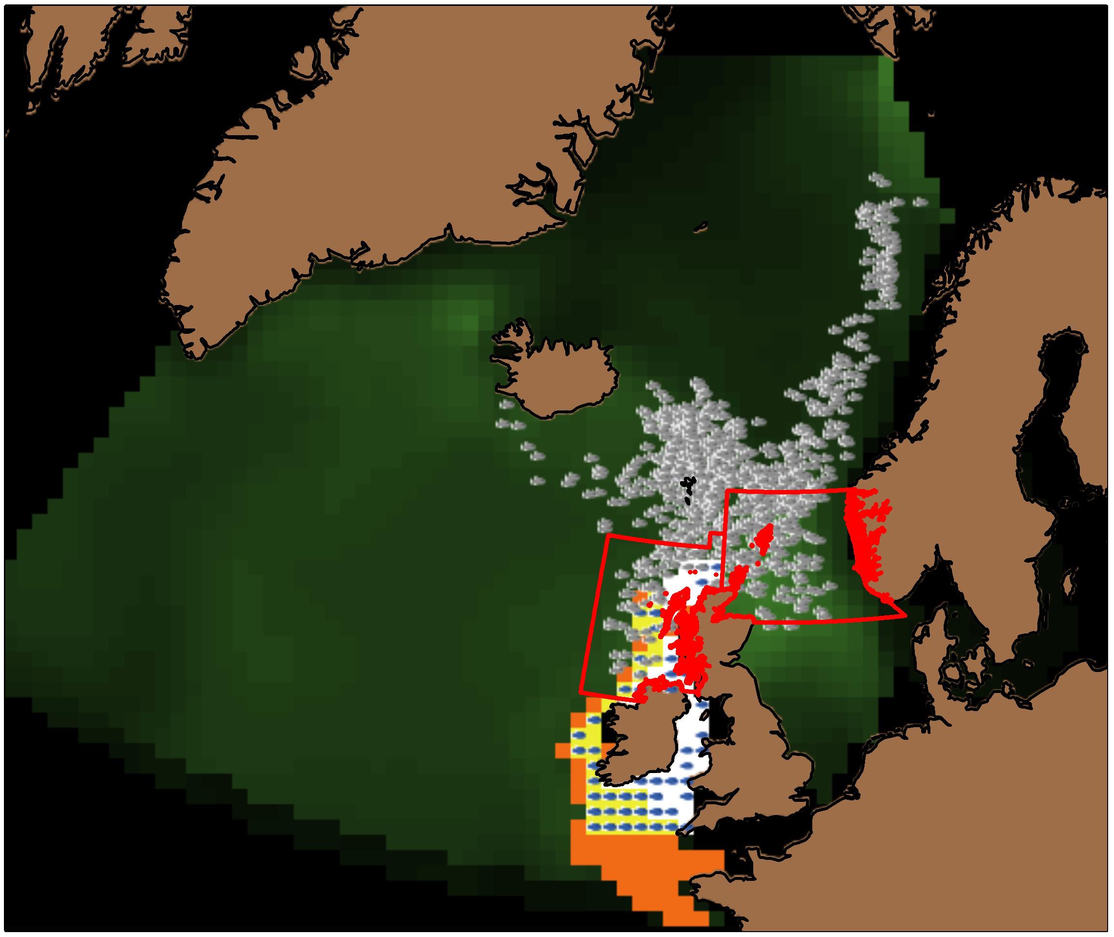
Figure 1. Snapshot of the IBM interface on August 1st 2009. Gray SIs in the Nordic and North Seas are adults, and blue SIs to the west of the British Isles are juveniles. The color of the landscape indicates phytoplankton density: darkest green equals 0 g m^–2 through light green which equals 3 g m^–2. Orange cells indicate potential spawning areas, white cells potential nursery areas, and yellow cells indicate areas that are both potential spawning and nursery areas. The nursery area is delimited by the 200 m isobath to the west of the British Isles, and the potential spawning area corresponds to the European shelf edge (−500 m < depth < −50 m). The red boxes (ICES divisions 6a and 4a) delimit the potential overwintering areas. The easternmost box (division 4a) is that which we close in our spatial management scenarios (see Table 2).

State Variables and Scales

The model landscape comprises a two-dimensional grid of patches of sea surface (Figure 1). The spatial extent spans from 47–77°N, and from −45° to 20°E. Each patch represents 60 × 60 km (Lambert Azimuthal equal area projection) and is characterized by prey density, sea surface temperature (SST), mackerel density, photoperiod and horizontal current velocities. The mackerel population is represented by a constant 4000 SIs; as n_cohort new SIs enter the model as juveniles each year, an equal number reach terminal age (> 15 years) and are removed from the model. While the number of SIs remains constant, the abundance that they represent differs; a SI’s abundance is determined by the level of recruitment in the year that it entered the model, and all subsequent mortality. Each SI is characterized by age, gender, life stage (egg, yolk-sac larvae, larvae, juvenile or adult), length, mass (structural, lipid and gonad), abundance and location. The temporal extent of the historical period spans from January 1st 2005 to December 31st 2018, and is extended to December 31st 2050 for projections. The model proceeds in discrete five-day time-steps.

Sub-models

In the following we give details of the IBM’s movement, bioenergetics and recruitment sub-models.

Movement

In broad terms, juveniles move randomly in nursery areas, and adults cycle between spawning, feeding and overwintering areas (see TRACE section 2 and Figure 1). For the purposes of this paper, we focus on the summer feeding period (July through September). We focus on this period because: (1) the summer distribution has recently expanded into the jurisdictions of Iceland and Greenland, which has complicated division of the catch allocation among states; and (2) we have recently validated an optimal-foraging model for this period (Boyd et al., 2020), outlined below.

In summer adults actively move in search of the most profitable patches on which to feed. Each patch is characterized by a profitability cue c_dd which is proportional to potential ingestion rate in that location. c_dd represents the bottom-up effect of phytoplankton density as a proxy for prey availability, a density-dependent effect of intraspecific competition, an effect of photoperiod (as NEAM are primarily visual feeders), and an effect of SST (Kelvins), in the form of a modified Beddington-DeAngelis (Beddington, 1975; DeAngelis et al., 1975) functional response:

$$c_{dd}=A\left(SST\right)p_{photo}\frac{X}{X+h+cD}(1)$$

where X is phytoplankton density (g m^–2), h is a half saturation constant, p_photo is photoperiod (as a proportion of 24 h) at the SI’s location, D is local mackerel density (g patch^–1), c determines the strength of the density dependence, and A(SST) is an Arrhenius function giving the effect of SST (see Eq. 2). h was estimated by fitting the IBM to data on NEAM SSB and weight-at-age using rejection approximate Bayesian computation (see section “IBM Calibration”). c was estimated using the same approach but in a previous application of the IBM (Boyd et al. submitted). A(SST) is given as:

$$A\left(SST\right)=e^{\frac{-E_a}{K}\left(\left(\frac{1}{SST}\right)-\left(\frac{1}{T_{ref}}\right)\right)}(2)$$

where E_a is an activation energy, K is Boltzmann’s constant and T_ref is an arbitrary reference temperature.

SIs move in search of the most profitable locations (Eq. 1) at which to feed following a gradient area search (GAS). The GAS algorithm is similar to that presented by Tu et al. (2012); Politikos et al. (2015), and Boyd et al. (2020). It should be noted that this model is a slight update to that presented in Boyd et al. (2020) as it now includes explicit effects of photoperiod and horizontal current velocities. See TRACE section 9 for a comparison of predicted and observed NEAM occurrence over summer. SIs can detect the profitability of the four neighboring patches in x and y dimensions. Positions are updated five times per time step (i.e., once per day) to ensure that SIs cannot overshoot the neighboring patch. Positions in x and y dimensions are updated in continuous space, as:

$$x_{t+1}=x_t+\left(D_x+R_x+C_x\right)$$

$$y_{t+1}=y_t+\left(D_y+R_y+C_y\right)(3)$$

where D_x and D_y denote directed movements toward the most profitable patches, R_x and R_y denote random movements, and C_x and C_y are displacements caused by zonal and meridional horizontal currents, respectively.

In the orientated component of Eq. (3) D_x and D_y, SIs compare the profitability at their current location with that of the day before. If it has become more profitable, they will continue to swim in the same direction as the directed component of their movement the day before. If a SI’s current environment is less profitable than the day before, it follows a gradient search toward what is perceived to be the most profitable patch based on information in x and y dimensions, at realized velocity V_r, given by:

$$D_x=V_r\frac{g_x}{\sqrt{g_x^2+g_y^2}}$$

$$D_y=V_r\frac{g_y}{\sqrt{g_x^2+g_y^2}}(4)$$

where g_x and g_y are the gradients of the profitability cues (Eq. 3) in x and y dimensions. V_r is given as minimum swimming velocity (V_min) plus random noise. V_min is as a function of body length L, as $V_{min}=a_v{L}^{b_v}{A}_r^{c_v}$, where a_v is a normalizing constant, b_v and c_v are scaling exponents, and A_r is the caudal fin aspect ratio (Sambilay, 1990). V_r is given by V_r=V_min+(V_minε), where ε is drawn randomly from a uniform distribution ranging from zero to one. The directed component of the GAS algorithm amounts to what is called a state-location orientation mechanism (basing new orientation on a comparison of the current and previous environment), and there is some indication that herring follow a similar strategy in the Norwegian sea (Fernö et al., 1998).

Following Politikos et al. (2015) we assume that movement is directed (D_x, D_y) for 12 h day^–1, and movement in the other 12 h follows the random component of Eq. (3), R_x, R_y, given as moving at velocity V_min in a random direction that is not southward. Random southward movement is not permitted because acoustic studies have shown that NEAM infrequently swim southwards over summer (Nøttestad et al., 2016). However, SIs may still move southward during the oriented component of the GAS algorithm (i.e., if feeding conditions are best on a more southerly patch), or due to currents. R_x and R_y introduce stochasticity into the GAS models and combine with the competition term in Eq. (1), cD, to prevent unrealistic overcrowding on optimal patches.

The effects of horizontal currents on SIs’ locations, C_x, C_y, are given as zonal (u) and meridional (v) current velocities (km h^–1), respectively, multiplied by the time step (here 24 h as the GAS model operates five times per 5 day time-step).

In addition to its effect on the perceived profitability of a patch (Eqs. 1, 2), SST delimits the possible modeled NEAM distribution. NEAM avoid areas in which temperature is below 7°C (Ólafsdóttir et al., 2018). To reflect this, SIs are deterred from moving to patches on which SST is below this threshold. In the directed component of Eq. (3), SIs are repelled from patches with SST < 7°C by setting profitability cues in those areas to 0. For the random component of Eq. (3), if a SI’s orientation would direct it on to a patch with SST < 7°C, its heading is reversed. If currents displace individuals on to an intolerably cold patch (or land) then this movement is abandoned and the SI instead moves to the centroid of the nearest suitable patch.

Bioenergetics

Individuals obtain energy from food X in the form of either phytoplankton (a proxy for baseline food availability) or smaller mackerel located on the same patch (see TRACE section 2 for size-based criteria that a SI must meet to be classed as potential prey). Over summer adults do not overlap with sufficient small mackerel, so in Eq. (1) X refers only to phytoplankton density. Energy uptake is proportional to Eq. (1). A proportion of the energy ingested from food is assimilated and made available to the vital processes maintenance (metabolic rate), growth, reproduction and energy storage. The rates at which energy is allocated to these processes depend on temperature and body size. The effect of temperature is generally given by the Arrhenius function (Eq. 2). The partitioning of energy to vital processes depends on an individual’s life stage and time of year. See Sibly et al. (2013) for an overview, and TRACE section 2 for full details. Note that, while adults allocate energy to reproduction, recruitment is modeled separately using a Ricker-style stock-recruitment model (see section “Recruitment”).

Movement-bioenergetics coupling

The energy cost of searching for food is subsumed into an individual’s active metabolic rate AMR. AMR is given as a function of SST, body mass M and swimming velocity V as:

$$AMR=a_{AMR}{M}^{b_{AMR}}{V}^{c_{AMR}}A(SST)(5)$$

where a_AMR is a normalizing constant, b_AMR and c_AMR are scaling exponents, and V is given by V = (V_r + V_min)/2, i.e., assuming that half of each day is spent at V_min, and half at V_r.

Recruitment

In this paper, recruitment is modeled differently than in previous applications of our IBM (Boyd et al., 2018, 2020). Here, we use a modified Ricker stock-recruitment function because it provides better fits to the latest recruitment estimates from the NEAM stock assessment. The Ricker model gives recruitment R as a function of SSB and average SST on the spawning grounds over the months March and April, as:

$$R=a_{R}SSB{e}^{-a_{R}SSB+b_{R}SST}(6)$$

where a_R and b_R were estimated by fitting Eq. (6) (in log-linear regression form, R² = 0.45) to data from the stock assessment. See TRACE section 3 for details of the Ricker model fitting process, variable importance and model diagnostics.

On December 31st each year, n_cohort new SIs (recruits) enter the model as juveniles at a random location in the nursery area, with abundance equal to R/n_cohort. Recruits’ body lengths set at the maximum length at the end of the first growth phase (20 cm, Villamor et al., 2004) minus ε 3 (cm), where ε is drawn randomly from a uniform distribution ranging from 0 to 1.

Emergent Properties

The movement and bioenergetics models describe the ways in which individuals’ characteristics (e.g., body mass, energy reserves, location) respond to their local food availability and SST. By summarizing the characteristics of all the individuals, we can obtain population measures. For example, SSB can be obtained by summing the individual body masses of all adults, and spatial distribution by summarizing the locations of the SIs.

Initialization

The IBM is initialized on 1 January 1995 using estimates of numbers-at-age from the stock assessment. This population is then apportioned into 4000 super-individuals such that there is an equal number of SIs in each year class. Body lengths are calculated from age using the standard von Bertalanffy equation, and energy reserves are set at half maximum. From these all other state variables are calculated when the simulation begins. Adults and juveniles are distributed randomly in the overwintering and nursery areas, respectively (see Figure 1). After initialization we allow the model to spin up from 1995–2005, after which point we begin to record outputs for model calibration. See TRACE section 2 for full details of initialization.

Model Forcing

In this section we describe the data used to force the IBM during the historical period 1 January 2005–31 December 2018.

Environmental Inputs

Environmental inputs to the model include maps of surface chlorophyll concentration, SST, horizontal current velocities and photoperiod. Chlorophyll and SST are derived from the global ESM GFDL-ESM-2M (Dunne et al., 2013; Geophysical Fluid Dynamics Laboratory, 2017). GFDL-ESM-2M has been identified as a suitable candidate for forcing fisheries and marine ecosystem models because: (1) it contains a relatively highly resolved representation of ocean biochemistry and its predictions correlate well with net primary productivity data; and (2) because model drift is negligible (Lotze et al., 2018; Tittensor et al., 2018). Environmental inputs are updated monthly. A slight complication arises in that the historical period as defined for CMIP (phase 5 as used here) ends in December 2005, after which RCP scenario-driven estimates are produced from the ESMs. This does not match the historical period as defined in this study (everything up to 2019). For this reason, from 2006 we had multiple environmental trajectories (one from each RCP) from which to choose as input to our IBM. Inspection of the environmental inputs revealed negligible divergence between fields of chlorophyll and SST out to 2019 from RCPs 2.6 and 8.5 (RMSEs of 0.31°C and 0.024 mg m^–2, respectively; see TRACE section 3). For this reason we simply took the mean of the environmental inputs from RCPs 2.6 and 8.5 as forcing to the IBM from 2006–2019.

Near surface (average over 0 to -30 m) horizontal current velocities were taken from the 1/3° OSCAR dataset (ESR 2009). Currents influence the movements of adults over summer (Eq. 4), so we obtained data for the months May through September. Outside of this period current velocities have no effect in the IBM. It would not be appropriate to include the effects of near surface current velocities on individuals outside of the summer period, when mackerel may inhabit deeper waters (e.g., −50 to −220 m over winter) (Jansen et al., 2012). Over summer NEAM are found in the upper water layer (average of ∼−20 m) (Nøttestad et al., 2016). As data are not available for the selected months prior to 2012, we generated mean climatologies for each month over 2012–2018. As such we do not account for inter-annual variability in current velocities.

Data on photoperiod (as a proportion of 24 h) at all latitudes in the IBM grid was extracted for each month using the daylength() function in the R package geosphere (Hijmans, 2019). Values correspond to the 15th day of each month, and are updated at the start of each month. All environmental data required processing for use in the IBM (e.g., re-gridding), the details of which can be found in TRACE section 3.

Fishing Mortality

As our IBM does not explicitly represent fleet dynamics, fishing mortality F is applied to the stock in a simple manner. Annual rates of F at age each year were taken from the 2019 NEAM stock assessment [ICES (2019b), extracted from stockassessment.org]. We incorporate monthly variation in F by setting the fraction of annual F in each month proportional to the mean historical fraction of annual NEAM catch taken in each month (see Table 1). Unless stated otherwise (see section “Spatial Management Scenarios”), F is applied uniformly to all individuals within an age group regardless of their location.

TABLE 1

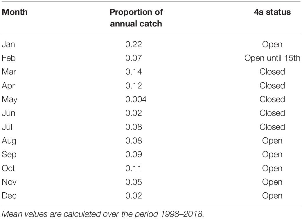
Table 1. Mean proportion of total annual catch taken in each month and whether or not division 4a is closed to fishing.

Future Scenarios

From 1 January 2019–31 December 2050 the IBM simulates the NEAM population under various scenarios, each with different assumptions about future climate and fishing pressure.

Climate Scenarios

We include two environmental scenarios representing the low and high levels of climate change mitigation action. Both scenarios comprise projections of chlorophyll and SST from GFDL-ESM-2M, with forcing from RCPs 2.6 and 8.5, i.e., low and high greenhouse gas emissions, respectively (see van Vuuren et al. (2011) for details). Current velocities remain as described in section “Environmental Inputs” in the future period for lack of available projections. It is important to note that we do not account for other climate-related stressors (e.g., ocean acidification).

Fishing Scenarios

For future fishing pressure we take mean F-at-age over the historical period 2001–2018 (Figure 2) and adjust it using one of three multipliers. The multipliers are used to set mean F over the most important age groups to the fishery (for NEAM 4–8 years) at one of three rates: F = 0; F_MSY (0.23 year^–1), i.e., the level of harvesting that is likely to result in maximum sustainable yield in the long-term; and F_lim (0.46 year^–1), i.e., high mortality used as an upper reference point (ICES, 2012, 2019c). F_lim is slightly larger than the highest F on record (ICES, 2019c). Monthly variation in F is implemented as in the historical period.

FIGURE 2

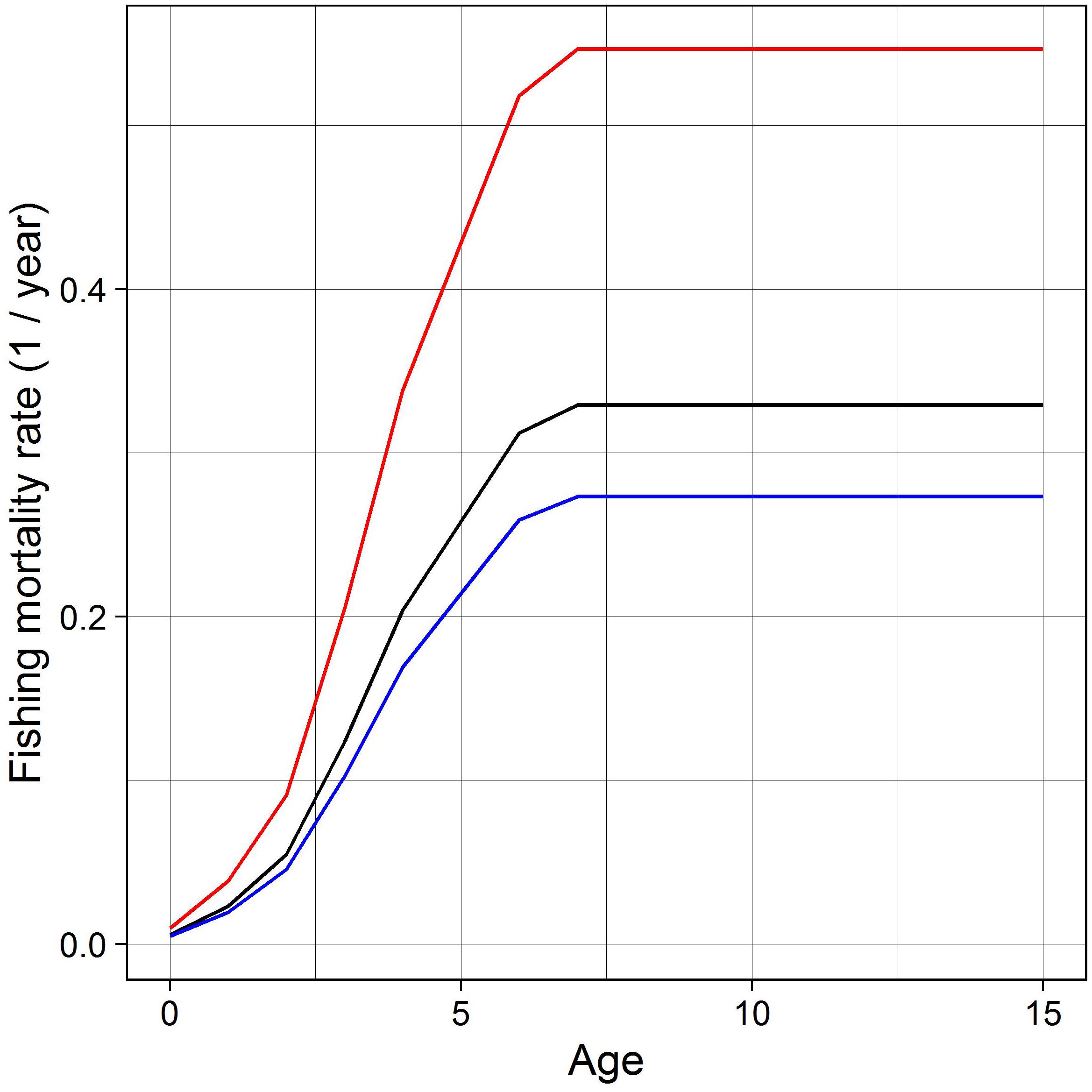
Figure 2. Mean F at age over 2001–2018 (black line), from which F_MSY (blue line) is calculated with a multiplier of 0.83, and F_lim (red line) with a multiplier of 1.66.

Spatial Management Scenarios

In addition to changes in annual F, we also simulate the consequences of two simple spatial management scenarios. Currently, no mackerel fishing is permitted the Northern North Sea (ICES division 4a, Figure 1) over the period 15 February to 31 July (ICES, 2019c). We simulate the possible consequences of a hypothetical measure in which this seasonal closure is extended to span the whole year. To do this we split fishing mortality into that which is applied inside 4a, and that which is applied outside. We then make assumptions about the amount of fishing mortality that will be redistributed from inside to outside of division 4a if it is closed. The first assumption is that none of the fishing mortality that would have taken place in division 4a is relocated, i.e., fishing mortality at age t F_t is set to zero inside division 4a when it is closed, but remains unchanged elsewhere. Under this assumption total F is reduced. The second assumption is that all of the fishing mortality that would have been inflicted in division 4a will be uniformly redistributed elsewhere. Under the second assumption F_t is raised outside of 4a to give redistributed fishing mortality at age t, F′_t, as:

$$F_t^{\prime }=F_t{\left(1-p_{in,t}\right)}^{-1}(7)$$

where p_in,t is the proportion of SIs in age group t that are inside division 4a in that time-step (see Yemane et al., 2009, for a similar approach). Under this assumption the spatial distribution of F changes, but the overall rate is unchanged. These scenarios are simplistic, but represent the extremes of possible fishery responses to area closures: relocating none or all of the fishing mortality. As such they give the bounds of possible outcomes.

Multi-Stressor Scenarios

To generate a range of future conditions for the NEAM stock, we combine the different assumptions about future climate and management decisions to generate nine multi-stressor scenarios. The first six scenarios represent each combination of RCP (2.6 and 8.5) and annual fishing mortality rate (unfished, F_MSY and F_lim). In these scenarios F is applied uniformly to all individuals within an age group. The final three scenarios represent the different assumptions about when ICES division 4a is closed to mackerel fishing, and if it is, how much of the fishing pressure that would have taken place inside is relocated elsewhere. For these latter scenarios we assume RCP = 8.5 and F = F_MSY. See Table 2 for a summary of the multi-stressor scenarios.

TABLE 2

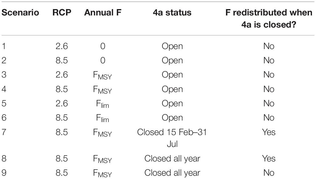
Table 2. Summary of the multi-stressor future scenarios.

IBM Calibration

We calibrated the half saturation constant (h in Eq. 1), i.e., the prey density at which ingestion rate reaches half maximum at a given temperature. h was estimated by fitting the IBM to data on SSB and weight-at-age using rejection approximate Bayesian computation (ABC) (van der Vaart et al., 2015) (see TRACE section 5 for model fits). In broad terms, we ran 2000 simulations while randomly sampling values of h from a uniform prior distribution. We then “accepted” the values of h that resulted in the best-fitting 30 simulations (1.5% tolerance), giving an approximation of its posterior distribution (see TRACE section 3 for full details of the ABC). To account for uncertainty in h, we simulated all future scenarios (Table 2) once for each of the 30 accepted parameter values.

IBM Simulations and Outputs

The IBM simulates the full life cycle of the NEAM population from 1 January 2005–31 December 2050. Simulations are forced by fishing mortality F at age, phytoplankton density X and SST. F is updated annually in the historical period, but remains constant in the future period. SST and phytoplankton density are updated monthly. From 2019 management and climate scenarios take effect (Table 2).

For the purposes of this paper, key outputs from the IBM are SSB (tonnes), annual catch (tonnes) from the fishery and mackerel density (tonnes km^–2) over the summer period (1 July to 30 September). SSB is calculated as the sum of the body masses of all mature individuals at spawning time (extracted 1 May). Catch is calculated is calculated cumulatively throughout each year from rates of fishing and natural mortality (see TRACE section 2), and mackerel biomass-at-age, using the standard Baranov equation (see TRACE section 2).

Results

Effect of Future Scenarios on SSB and Yield

To test how the NEAM stock size and associated yield from the fishery may respond to future climate change and management options, we compared future SSB and annual catch from multi-stressor scenarios 1–6 (Table 2 and Figure 3). For both SSB and catch we present means over the period 2021–2050. Our results show that, for both SSB and catch, the choice of fishing mortality has a significant effect (ANOVA, p < 0.01). As expected SSB increases as rates of fishing mortality are lowered. The effect of management decision on catch is more subtle. There is a significantly higher catch under F_lim than under F_MSY where RCP = 8.5 (paired t-test, p < 0.05, mean difference of 0.03 million tons), but the mean difference is not statistically significant in the RCP 2.6 scenario (0.009 million tons, p > 0.05). Within the F_lim and F_MSY scenarios, SSB is greater in the RCP 8.5 scenarios (paired t tests, p < 0.05, mean differences of 0.48 and 0.33 million tons, respectively). Within the F_lim and F_MSY scenarios catch was also higher in the RCP 8.5 scenario (mean differences of 0.10 and 0.08 million tons, respectively). Overall, the effect of fishing mortality appears much greater than that of climate over the range of scenarios considered (discussed in section “Discussion”).

FIGURE 3

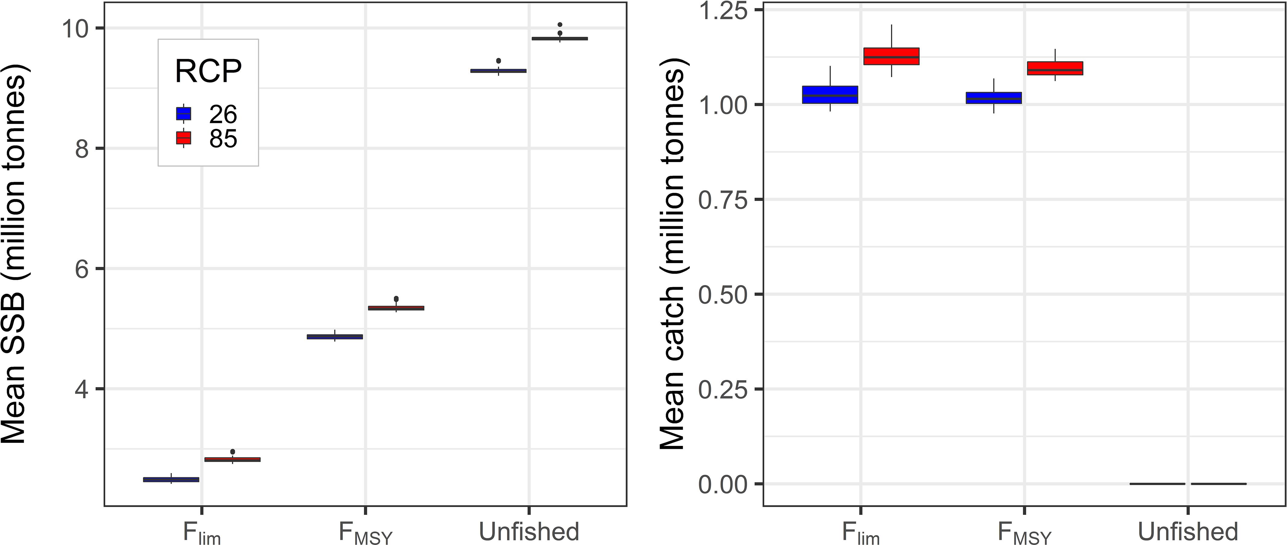
Figure 3. Left: Mean SSB at spawning time over the period 2021–2050; and right: mean annual catch from the fishery over the same period. From left to right within each panel, boxes represent scenarios 1–6 (Table 2). Within management scenarios the left-hand boxes correspond to RCP 2.6 and the right-hand boxes to RCP 8.5. Boxplots show medians and interquartile ranges, with the spread representing uncertainty in the parameter h and stochasticity in the IBM.

Effect of Future Scenarios on the Summer Feeding Distribution

To test how the summer feeding distribution of NEAM may change in future, we compare mean mackerel density in July- September over 2005–2010, with that over 2045–2050, for each of scenarios 1–6 (Figure 4). There are positive anomalies in the North East region south of Svalbard in all scenarios, with the most pronounced increases of ∼ 400 tons km^–2 in the unfished scenarios. Increased density in these regions is expected because warming opens up new habitat in the North. Another expected finding is that, in the unfished and F_MSY scenarios, there are positive anomalies in the western region south and East of Iceland. Again, these anomalies are most pronounced in the unfished scenario (up to ∼ 200 tons km^–2). This can be explained by an increase in stock size in these scenarios, most notably in the unfished scenario (Figure 3). Increasing stock size provides an incentive to move further from the traditional feeding area (Norwegian Sea) in search of areas in which competition for food is less intense (due to the density term, cD, in Eq. 1). Aside from these expected results, the distribution changes are not intuitive. Reasons for this are discussed in section “Discussion.”

FIGURE 4

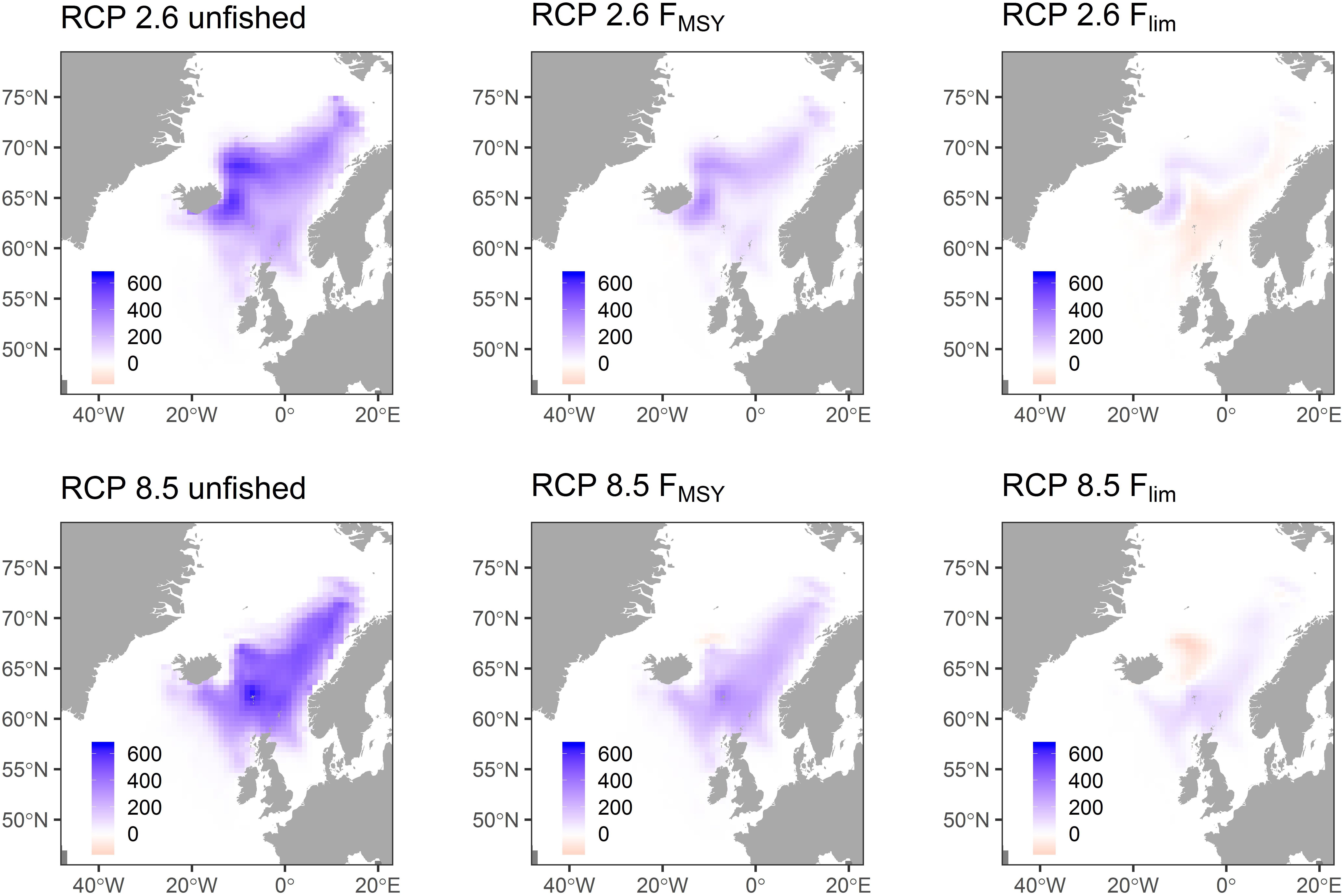
Figure 4. Change in mean mackerel density (tonnes km^–2) between the start and end of a simulation for scenarios 1–6 (Table 2). Start is taken as the mean over 2005–2010, and end as the mean over 2045–2050.

Effect of Spatial Management Scenarios

To show how it may be possible to simulate the effects of spatial management options, in Figure 5 we compare predictions of mean SSB and catch over the period 2021–2050 from a baseline scenario that represents the current situation (2019), to those from two alternative scenarios. The hypothetical scenarios both represent an extension from a seasonal to permanent closure in ICES division 4a, with different assumptions about how much fishing pressure is relocated elsewhere when it is closed (details in Figure 5 caption). As expected, we found that if fishing mortality is relocated outside division 4a when it is closed, then future SSB does not differ from the baseline scenario (paired t-test, p > 0.05, mean difference of 0.10 million tons). However, if fishing mortality is not redistributed when division 4a is closed, then future SSB is significantly higher than the baseline scenario (paired t-test, p < 0.05, mean difference of 1.04 million tons). To gauge the consequences of each scenario for the fishery we also present future catch in Figure 5. It can be seen that closing division 4a for the entire year without redistributing fishing mortality would result in a significantly lower yield for the fishery (paired t-test p < 0.05, mean difference of 0.11 million tons). In summary, these results show that closing division 4a could increase NEAM SSB, but that this will depend on the response of the fishers in terms of how much F is redistributed. A reduction in catch when F is not redistributed suggests that fishers would be likely to redistribute their effort elsewhere should legislation allow it.

FIGURE 5

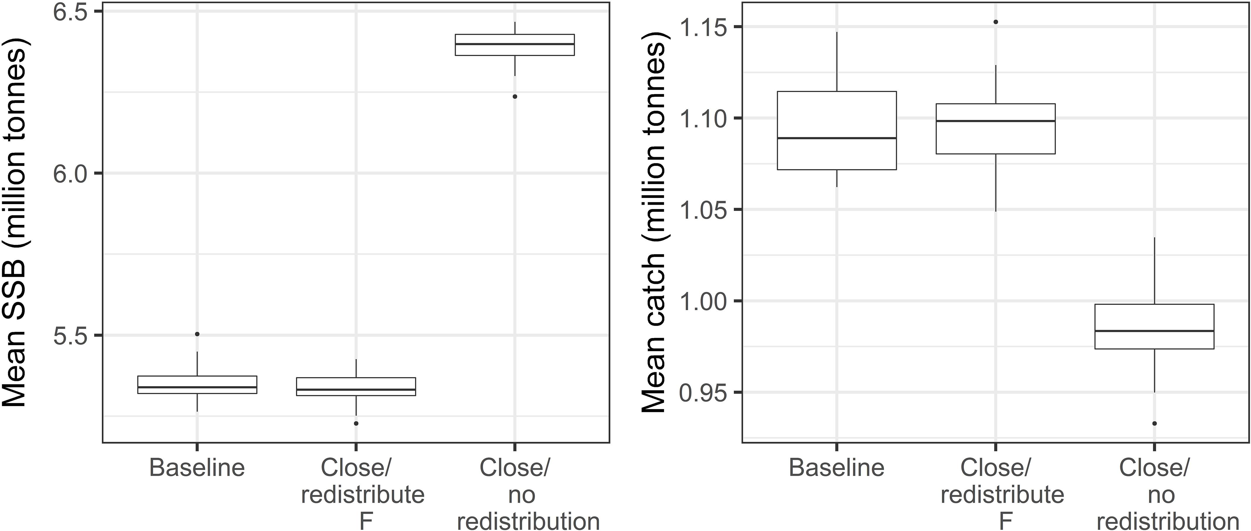
Figure 5. Mean SSB (left panel) and annual catch (right panel) over the period 2021–2050 under three scenarios: (1) baseline, i.e., ICES division 4a is closed from February 15th to July 31st as at present (2019) and F is raised elsewhere to account for this; (2) division 4a is closed for the entire year and F is raised elsewhere to account for this; and (3) division 4a is closed all year and F is not redistributed, i.e., there is an overall reduction in F. Boxplots show medians and interquartile ranges, representing variability arising from stochasticity the IBM and uncertainty in the parameter h.

Discussion

Using an existing spatially explicit IBM, we have simulated NEAM population dynamics and yield from the fishery out to 2050 under a range of climate and fishing scenarios. Environmental inputs to the IBM were obtained from the ESM GFDL-ESM-2M assuming high and low levels of climate change mitigation action. Management scenarios comprised a range of levels of fishing mortality F. After testing the effects of these simple management scenarios, we then implemented an extension to an existing seasonal fishery closure in the Northern North Sea, assuming a moderate level of F and low climate mitigation action. We further divided this spatial scenario by making assumptions about how much of the fishing mortality that would have been inflicted in the Northern North Sea is relocated elsewhere when it is closed. Our results suggest that, over the range of scenarios considered, the effects of fishing mortality are greater than those of climate. These results hold in terms of future SSB, yield from the fishery and the extent to which the summer distribution changes. We then showed that closing an area to fishing may have positive effects for a stock, but that this is highly dependent on how the fishery responds in terms of whether or not fishing is relocated elsewhere.

In this paper we have taken a single-species approach primarily because it allowed us to incorporate sensible assumptions about future fishing mortality. We were able to force the IBM with plausible rates of fishing mortality, including a crude representation of its spatial distribution (e.g., inside or outside of division 4a) and intra-annual variation, as well as the relative catchability of different age groups. This would be difficult to achieve for numerous species or functional groups represented in, for example, ecosystem models. Second, we have extensively validated our IBM using data on population dynamics, structure and spatial distribution (Boyd et al., 2018, 2020). Again, because more holistic models represent numerous species or functional groups, it would be difficult to achieve the same level of validation for a single species. There are, however, processes that single-species models cannot include, notably interspecific competition and predation (Hollowed et al., 2000). NEAM cohabit the Nordic Seas with herring and blue whiting in the summer months. There are contrasting reports over the degree to which the species’ diets overlap (Langøy et al., 2012; Bachiller et al., 2016), but recent work has shown that herring larvae are an important prey for NEAM (Skaret et al., 2015). Moreover, herring stock size may affect the distribution of NEAM over summer (Nikolioudakis et al., 2018). When interpreting our results, it is important to keep in mind that our IBM does not account for interspecific interactions.

Our results suggest that, while climate is important, fishing intensity is likely to have a much larger effect on the NEAM stock out to 2050. This result is evident both in terms of SSB (Figure 3), and the degree to which the summer distribution changes (Figure 4). There are four possible explanations for this finding. First, the relative impacts of climate and fishing depend on the choice of scenarios. Inclusion of an “unfished” scenario is extreme and would be expected to result in a dramatic increase in SSB (note there is no equivalent zero emissions scenario). However, between the more plausible F_MSY and F_lim scenarios, the effect of fishing remains much greater than that of climate. Second, the western spawning component of NEAM may less susceptible to the effects of climate due to its latitudinal position within the species’ thermal niche. It has been shown that populations inhabiting the cooler parts of their species’ distribution are less negatively or more positively affected by increasing temperature than those in the warmer regions (Free et al., 2019). Atlantic mackerel are found as far south as Morocco (Trenkel et al., 2014), meaning that the western spawning component of NEAM represents one of the northernmost sub-units of the stock. Another possibility is that the effect of climate is smaller than fishing due to the oceanographic regime in the North Atlantic. The ensemble of ESMs participating in CMIP indicate that the region to the east of Greenland and south of Iceland will not exhibit a significant increase in SST out to 2100 (Alexander et al., 2018). This could be explained by a weakening of the Atlantic meridional overturning circulation (AMOC) which results in reduced poleward transport of warm water in the Atlantic (Alexander et al., 2018). Indeed, simulations using an ensemble of 10 ESMs predict a weakening of AMOC out to 2100, with the most marked weakening (15–60%) under RCP 8.5 (Cheng et al., 2013). Finally, the relatively small change in the NEAM stock between climate scenarios may reflect the time period chosen in our study. Projections of SST from the CMIP ensemble begin to diverge around the mid-twenty-first century (Hutchings et al., 2012, Supplementary Figure S22), and the same is true for the projections used here (see TRACE section 3). It is possible that the effect of climate on the NEAM would increase if simulations were conducted further into the future.

Within fishing scenarios the IBM predicts highest SSB, and hence catch, under RCP 8.5. This is largely down to the positive relationship between SST and recruitment included in the stock-recruitment model. Recruitment is almost always positively correlated with temperature for species inhabiting the cooler regions of their thermal niche (Myers, 1998). So, while the western component of the NEAM stock continues to spawn in cooler regions than e.g., the southern component, the sign of this relationship is likely to hold. This could have important implications for the NEAM fishery if warming waters make sustainable management easier. However, such inferences should be made with extreme caution because we do not know if this positive relationship will break down as waters warm. At some temperature the relationship will shift from positive to negative and this is not accounted for in our IBM (because we are not able to establish the limit from historical data). If the positive effect of temperature on recruitment ceases due to warming in the North East Atlantic over the time period considered, then our projections may be optimistic.

The main caveat of our approach is that we use a single ESM to provide inputs to a single ecological model. As a result, our predictions do not account for structural uncertainty—arising from what processes are represented and by what functional forms-in either of the models (Spence et al., 2018). We chose to use the ESM GFDL-ESM-2M (Dunne et al., 2013) to provide environmental forcing to our IBM because it has previously been identified as suitable for this purpose as part of FISH-MIP (Tittensor et al., 2018). Of particular relevance to our study is that the GFDL ESM has a relatively well-developed biogeochemical formulation and correlates well with primary productivity data (Tittensor et al., 2018). In addition to GFDL-ESM-2M another ESM, IPSL-CM5A-LR, was identified by FISH-MIP as a suitable candidate for forcing marine ecosystem models. We attempted to include inputs from the IPSL ESM but found that an under-prediction of SST on the NEAM spawning grounds led to frequent recruitment failures in our IBM. With respect to the fish population model, we are aware of other IBMs representing NEAM (Utne et al., 2012; Heinänen et al., 2018). However, to our knowledge these IBMs were designed primarily to represent the stock’s spatial distribution and do not make multi-generational predictions of stock size. For this reason, they cannot make predictions about how the stock may develop in future. While we do not account for variation in model structures, we have included a wide range of possible future conditions in terms of climate and harvesting regimes.

While our IBM captures some of the key individual level processes that relate fish population dynamics to prey availability and temperature, there are other climate-related stressors that it does not account for. First, the ocean is projected to become more acidic over the twenty-first century (Holsman et al., 2018). It is thought that ocean acidification will have deleterious effects on fish stocks, such as increased larval mortality and reduced recruitment (Stiasny et al., 2016). Second, ocean oxygen concentration is declining (deoxygenation) in response to increasing temperature (Breitburg et al., 2018). Oxygen concentration affects rates of energy expenditure, such as growth and metabolism (e.g., Del Toro-Silva et al., 2008), which is not accounted for in our bioenergetics model. Third, our IBM uses fields of chlorophyll concentration as a proxy for prey availability. Use of chlorophyll concentration does not account for potential changes to the composition of prey which may occur under novel environmental conditions (Holsman et al., 2018). This may reduce the predictive power of our IBM if NEAM vital rates depend on the composition of available prey. Indeed, S. scombrus recruitment appears to be related to the prevalence of large copepods such as Calanus species (Ringuette et al., 2002; Jansen, 2016). This is also a problem in that zooplankton is expected to decline at a greater rate than phytoplankton (negative amplification) (Chust et al., 2014), and the pathways of energy transfer from primary producers to e.g., pelagic or benthic food-webs may change, partly in response to the composition of the primary producers themselves (Van Denderen et al., 2018). For these reasons our assumption that chlorophyll concentration is near proportional to prey availability may not hold. Finally, while our IBM captures broad scale effects of prey availability and temperature on the NEAM stock, use of environmental fields derived from a global ESM limited our study to a relatively coarse (60 km²) spatial resolution (even working at this resolution required some downscaling of the ESM outputs, see TRACE section 3). For this reason our IBM is unable to capture mesoscale processes, such as fronts, that could affect the distribution and productivity of the NEAM stock (Sato et al., 2018). In all, our IBM accounts only for broad scale effects of temperature and a proxy for prey availability on NEAM physiology and behavior, and the results should be interpreted with this in mind.

In addition to stock size, the future distribution of NEAM over summer is an important output from our IBM. Over recent years the summer feeding distribution of NEAM has expanded from its traditional core in the Norwegian Sea, north and westward into the jurisdictions of Iceland and Greenland (Berge et al., 2015; Pacariz et al., 2016; Nikolioudakis et al., 2018; Ólafsdóttir et al., 2018). This has caused political disputes over how the catch should be allocated among coastal states in the region (Hannesson, 2018). Our IBM predicts a north-and westward expansion of the NEAM summer distribution under the F_MSY and unfished scenarios (Figure 4 and see Supplementary Figure S22). This finding is expected because under these scenarios SSB increases which forces SIs to the northern and western fringes of the distribution where competition for food is less intense. However, the IBM does not predict an increase in density in Greenlandic waters out to 2050, where NEAM have been present in large densities since ca. 2012 (Ólafsdóttir et al., 2018). This discrepancy cannot be explained by e.g., temperature, which remains suitable for NEAM in this region in all scenarios, but rather reflects the assumptions made in our IBM. First, our foraging model assumes that SIs move in response to local gradients in feeding opportunities (reactive orientation). Under this assumption SIs do not reach Greenlandic waters in appreciable numbers. It may be the case that NEAM use a combination of reactive and predictive orientation, i.e., where individuals move toward areas that are predicted to be best, when foraging. Indeed, Nøttestad et al. (2016) suggest that NEAM may use current direction as a cue on which to base predictive orientation. Another possibility is that changes in the spawning distribution, which occurs in spring directly before feeding, could influence the summer distribution. The spawning distribution of NEAM has changed in the past (Hughes et al., 2014) and will likely change in future (Bruge et al., 2016), which is not captured fully by our IBM (spawning is constrained by temperature but only occurs on the European shelf edge). An individuals’ location once spent after spawning is equivalent to its starting point for the feeding migration so could influence the subsequent distribution over summer. Our IBM can reproduce the summer distribution from Norway in the East to Iceland in the west with high skill (Boyd et al., 2020), but its predictions of NEAM density west of Iceland should be viewed with caution.

Generally speaking species’ distributions are expected to shift poleward as temperature increases (Hughes et al., 2014; Bruge et al., 2016; Pacariz et al., 2016). However, our IBM predicts more nuanced effects of climate on the NEAM summer distribution. For example, density anomalies are more positive in the northern regions under RCP 2.6, which is usually associated with cooler conditions, than under RCP 8.5. Moreover, there are negative anomalies in the northern Norwegian Sea under the RCP 8.5 F_lim scenario, but not in the equivalent RCP 2.6 scenario. These results can be explained by a slight cooling of surface waters in these regions under RCP 8.5, which may reflect the enhanced weakening of AMOC under RCP 8.5 (Cheng et al., 2013). In summary, there are some intuitive changes to the NEAM summer distribution (e.g., expansion when stock size is high) out to 2050, but a weakening of AMOC could result in more unexpected distribution patterns.

In addition to changes in rates of total fishing mortality, we also simulated the effects of a hypothetical extension to a fishery closure in the Northern North Sea. To do this we made two simple assumptions about the redistribution of fishing mortality from inside to outside of the area when it is closed. Our results show that predicted stock size and yield from the fishery are highly sensitive to these assumptions (Figure 5). This result is intuitive, and as much as our model in its current form can say, but does highlight the potential value of modeling fishing pressure explicitly. Strides are being made toward development of socio-economic IBMs [or, as they are known in this field, agent-based models (ABMs)] in which fishing pressure emerges from the decisions of individual fishers (Lindkvist et al., 2020). To date, these socio-economic ABMs have been coupled to simple models of fish population dynamics, such as a simple logistic growth models (e.g., Bailey et al., 2019). In future socio-economic ABMs could be coupled to biological IBMs such as ours, providing a detailed description of the human-environment system. Then, variables such as the amount of fishing pressure that is redistributed from inside to outside an area if it is closed to fishing (as in our simple scenario), or how the spatial distribution of fishing effort may change in response to changes in a stock’s distribution, would emerge. Indeed, the NEAM fishery, with its associated geopolitical issues, may provide an interesting candidate for studying the coupling of fisher behavior and fish stock dynamics.

In summary, we feel that our results give valuable, broad-scale insight into the ways in which the NEAM stock may respond to climate and management scenarios. By simulating the stock under a range of scenarios spanning the extremes of climate mitigation action and fishing pressure, we hope to have given some indication of the bounds of possible future responses. We would like to stress, however, that our results are not intended to be used in a decision-making context; such long-term projections come with too much uncertainty for use in tactical management. It is possible that our projections are optimistic as we do not account for e.g., ocean acidification, deoxygenation and changes in the composition of prey, all of which could have deleterious effects on the NEAM stock. Going forward it would be useful to extend our approach and incorporate: (1) additional species in the IBM, such as herring and blue whiting (though this will be time-consuming); (2) some representation of fleet dynamics and fisher behavior in order to make more realistic predictions about the effects of spatial management options; and (3) additional climate-related stressors such as ocean acidification, deoxygenation and changes in prey composition.

Data Availability Statement

All datasets generated for this study are included in the article/Supplementary Material.

Author Contributions

RB led the model development and writing of the manuscript. All authors contributed conceptually to the study design and gave critical comments on the manuscript.

Funding

This work was supported by the NERC Ph.D. studentship (Grant No. NE/L002566/1) with CASE sponsorship from CEFAS.

Conflict of Interest

The authors declare that the research was conducted in the absence of any commercial or financial relationships that could be construed as a potential conflict of interest.

Acknowledgments

We would like to thank Andrew Campbell for providing us with NEAM catch data and Richard Nash for his helpful comments on this manuscript.

Supplementary Material

The Supplementary Material for this article can be found online at: https://www.frontiersin.org/articles/10.3389/fmars.2020.00639/full#supplementary-material

DATA SHEET S1 | TRACE.

DATA SHEET S2 | Scenarios 1 to 6.

DATA SHEET S3 | Scenarios 7 to 9.

Footnotes

1. ^ www.fishforecasts.dtu.dk/forecasts

References

Alexander, M. A., Scott, J. D., Friedland, K. D., Mills, K. E., Nye, J. A., Pershing, A. J., et al. (2018). Projected sea surface temperatures over the 21st century: changes in the mean, variability and extremes for large marine ecosystem regions of Northern Oceans. Elem. Sci. Anth. 6:9. doi: 10.1525/elementa.191

CrossRef Full Text | Google Scholar

Bachiller, E., Skaret, G., Nøttestad, L., and Slotte, A. (2016). Feeding ecology of Northeast Atlantic mackerel, Norwegian spring-spawning herring and blue whiting in the Norwegian Sea. PLoS One 11:e0149238. doi: 10.1371/journal.pone.0149238

PubMed Abstract | CrossRef Full Text | Google Scholar

Bailey, R. M., Carrella, E., Axtell, R., Burgess, M. G., Cabral, R. B., Drexler, M., et al. (2019). A computational approach to managing coupled human–environmental systems: the POSEIDON model of ocean fisheries. Sustain. Sci. 14, 259–275. doi: 10.1007/s11625-018-0579-9

CrossRef Full Text | Google Scholar

Beddington, J. R. (1975). Mutual interference between parasites or predators and its effect on searching efficiency. J. Anim. Ecol. 44, 331–340. doi: 10.2307/3866

CrossRef Full Text | Google Scholar

Berge, J., Heggland, K., Lønne, O. J., Cottier, F., Hop, H., Gabrielsen, G. W., et al. (2015). First records of Atlantic mackerel (Scomber scombrus) from the Svalvard Archipelago, Norway, with possible explanations for the extension of its distribution. Arctic 68, 54–61. doi: 10.14430/arctic4455

CrossRef Full Text | Google Scholar

Borja, A., Uriarte, A., and Egana, J. (2002). Environmental factors and recruitment of mackerel, Scomber scombrus L. 1758, along the north-east Atlantic coasts of Europe. Fish. Oceanogr. 11, 116–127. doi: 10.1046/j.1365-2419.2002.00190.x

CrossRef Full Text | Google Scholar

Boyd, R., Roy, S., Sibly, R., Thorpe, R., and Hyder, K. (2018). A general approach to incorporating spatial and temporal variation in individual-based models of fish populations with application to Atlantic mackerel. Ecol. Modell. 382, 9–17. doi: 10.1016/j.ecolmodel.2018.04.015

CrossRef Full Text | Google Scholar

Boyd, R., Sibly, R. M., Hyder, K., Thorpe, R. B., Walker, N. D., and Roy, S. (2020). Simulating the summer feeding distribution of Northeast Atlantic mackerel with a mechanistic individual-based model. Prog. Oceanogr. 183:102299. doi: 10.1016/j.pocean.2020.102299

CrossRef Full Text | Google Scholar

Breitburg, D., Levin, L. A., Oschlies, A., Grégoire, M., Chavez, F. P., Conley, D. J., et al. (2018). Declining oxygen in the global ocean and coastal waters. Science 359:eaam7240. doi: 10.1126/science.aam7240

PubMed Abstract | CrossRef Full Text | Google Scholar

Brochier, T., Ecoutin, J. M., de Morais, L. T., Kaplan, D. M., and Lae, R. (2013). A multi-agent ecosystem model for studying changes in a tropical estuarine fish assemblage within a marine protected area. Aquat. Living Resour. 26, 147–158. doi: 10.1051/alr/2012028

CrossRef Full Text | Google Scholar

Bruge, A., Alvarez, P., Fontán, A., Cotano, U., and Chust, G. (2016). Thermal niche tracking and future distribution of atlantic mackerel spawning in response to ocean warming. Front. Mar. Sci. 3:86. doi: 10.3389/fmars.2016.00086

CrossRef Full Text | Google Scholar

Cheng, W., Chiang, J. C. H., and Zhang, D. (2013). Atlantic meridional overturning circulation (AMOC) in CMIP5 Models: RCP and historical simulations. J. Clim. 26, 7187–7197. doi: 10.1175/JCLI-D-12-00496.1

CrossRef Full Text | Google Scholar

Chust, G., Allen, J. I., Bopp, L., Schrum, C., Holt, J., Tsiaras, K., et al. (2014). Biomass changes and trophic amplification of plankton in a warmer ocean. Glob. Chang. Biol. 20, 2124–2139. doi: 10.1111/gcb.12562

PubMed Abstract | CrossRef Full Text | Google Scholar

DeAngelis, D. L., Goldstein, R. A., and O’Neill, R. V. (1975). A model for tropic interaction. Ecology 56, 881–892. doi: 10.2307/1936298

CrossRef Full Text | Google Scholar

Del Toro-Silva, F. M., Miller, J. M., Taylor, J. C., and Ellis, T. A. (2008). Influence of oxygen and temperature on growth and metabolic performance of Paralichthys lethostigma (Pleuronectiformes: Paralichthyidae). J. Exp. Mar. Bio. Ecol. 358, 113–123. doi: 10.1016/j.jembe.2008.01.019

CrossRef Full Text | Google Scholar

Dunne, J. P., John, J. G., Shevliakova, S., Stouffer, R. J., Krasting, J. P., Malyshev, S. L., et al. (2013). GFDL’s ESM2 global coupled climate-carbon earth system models. Part II: Carbon system formulation and baseline simulation characteristics. J. Clim. 26, 2247–2267. doi: 10.1175/JCLI-D-12-00150.1

CrossRef Full Text | Google Scholar

Fernö, A., Pitcher, T. J., Melle, W., and Nøttestad, L. (1998). The challenge of the herring in the Norwegian Sea: making optimal collective spatial decisions. Sarsia 83, 149–167. doi: 10.1080/00364827.1998.10413679

CrossRef Full Text | Google Scholar

Free, C. M., Thorson, J. T., Pinsky, M. L., Oken, K. L., Wiedenmann, J., and Jensen, O. P. (2019). Impacts of historical warming on marine fisheries production. Science 363, 979–983. doi: 10.1126/science.aau1758

PubMed Abstract | CrossRef Full Text | Google Scholar

Geophysical Fluid Dynamics Laboratory (2017). WCRP CMIP5: Geophysical Fluid Dynamics Laboratory (GFDL) GFDL-ESM2M Model Output Collection. Princeton, NJ: Geophysical Fluid Dynamics Laboratory.

Google Scholar

Goethel, D. R., Quinn, T. J., and Cadrin, S. X. (2011). Incorporating spatial structure in stock assessment: movement modeling in marine fish population dynamics. Rev. Fish. Sci. 19, 119–136. doi: 10.1080/10641262.2011.557451

CrossRef Full Text | Google Scholar

Gregg, W. W., Conkright, M. E., Ginoux, P., O’Reilly, J. E., and Casey, N. W. (2003). Ocean primary production and climate: global decadal changes. Geophys. Res. Lett. 30:1809. doi: 10.1029/2003GL016889

CrossRef Full Text | Google Scholar

Grimm, V., Berger, U., Bastiansen, F., Eliassen, S., Ginot, V., Giske, J., et al. (2006). A standard protocol for describing individual-based and agent-based models. Ecol. Modell. 198, 115–126. doi: 10.1016/j.ecolmodel.2006.04.023

CrossRef Full Text | Google Scholar

Hall, S. J. (2001). “The use of technical measures in responsible fisheries: area and time restrictions,” in A Fishery Manager’s Guidebook, eds K. L. Cochrane and S. M. Garcia (Hoboken, NJ: Wiley).

Google Scholar

Halpern, B. S., Diamond, J., Gaines, S., Gelcich, S., Gleason, M., Jennings, S., et al. (2012). Near-term priorities for the science, policy and practice of Coastal and Marine Spatial Planning (CMSP). Mar. Policy 36, 198–205. doi: 10.1016/j.marpol.2011.05.004

CrossRef Full Text | Google Scholar

Hannesson, R. (2018). Shared stocks, game theory and the zonal attachment principle. Fish. Res. 203, 6–11. doi: 10.1016/j.fishres.2017.07.026

CrossRef Full Text | Google Scholar

Heinänen, S., Chudzinska, M. E., Brandi Mortensen, J., Teo, T. Z. E., Rong Utne, K., Doksæter Sivle, L., et al. (2018). Integrated modelling of Atlantic mackerel distribution patterns and movements: a template for dynamic impact assessments. Ecol. Modell. 387, 118–133. doi: 10.1016/j.ecolmodel.2018.08.010

CrossRef Full Text | Google Scholar

Henson, S., Cole, H., Beaulieu, C., and Yool, A. (2013). The impact of global warming on seasonality of ocean primary production. Biogeosciences 10, 4357–4369. doi: 10.5194/bg-10-4357-2013

CrossRef Full Text | Google Scholar

Hijmans, R. J. (2019). geosphere: Spherical Trigonometry. R package version 1.5–10. Available online at: https://CRAN.R-project.org/package=geosphere

Google Scholar

Hollowed, A. B., Bax, N., Beamish, R., Collie, J., Fogarty, M., Livingston, P., et al. (2000). Are multispecies models an improvement on single-species models for measuring fishing impacts on marine ecosystems? ICES J. Mar. Sci. 57, 707–719. doi: 10.1006/jmsc.2000.0734

CrossRef Full Text | Google Scholar

Holsman, K., Hollowed, A., Ito, S., Bograd, S., Hazen, E., King, J., et al. (2018). “Climate change impacts, vulnerabilities and adaptations: North Pacific and Pacific Arctic marine fisheries,” in Impacts of Climate Change on Fisheries and Aquaculture: Synthesis of Current Knowledge, Adaptation and Mitigation Options, eds M. Barange, T. Bahri, M. Beveridge, K. Cochrane, S. Funge-Smith, and F. Poulain (Rome: FAO), 113–138.

Google Scholar

Hughes, K. M., Dransfeld, L., and Johnson, M. P. (2014). Changes in the spatial distribution of spawning activity by north-east Atlantic mackerel in warming seas: 1977–2010. Mar. Biol. 161, 2563–2576. doi: 10.1007/s00227-014-2528-1

CrossRef Full Text | Google Scholar

Hutchings, J. A., Cote, I., Dodson, J., Fleming, I., Jennings, S., Mantua, N., et al. (2012). Canada’s international and national commitments to sustain marine biodiversity. Environ. Rev. 20, 312–352. doi: 10.1139/a2012-013

CrossRef Full Text | Google Scholar

ICES (2012). 1.7 Acronyms and Terminology. Copenhagen: ICES.

Google Scholar

ICES (2014a). Report of the Benchmark Workshop on Pelagic Stocks (WKPELA). Copenhagen: ICES.

Google Scholar

ICES (2014b). Report of the Report of the Working Group on Widely Distributed Stocks (WGWIDE) report 2014. Copenhagen: ICES, 37–192.

Google Scholar

ICES (2017). Ices Wgwide Report. Copenhagen: ICES, 356–503.

Google Scholar

ICES (2019a). ICES Wgwide Report. Copenhagen: ICES, 21–27.

Google Scholar

ICES (2019b). Mackerel (Scomber scombrus) in subareas 1–8 and 14, and in Division 9.a (the Northeast Atlantic and adjacent waters). ICES Advice Fish. Oppor. Catch, Effort. Copenhagen: ICES.

Google Scholar

ICES (2019c). Norway Special Request For Revised 2019 Advice on Mackerel (Scomber scombrus) in Subareas 1 – 8 and 14, and in Division 9.a (the Northeast Atlantic and Adjacent Waters). Copenhagen: ICES, 1–17.

Google Scholar

Jansen, T. (2014). Pseudocollapse and rebuilding of North Sea mackerel (Scomber scombrus). ICES J. Mar. Sci. 71, 299–307. doi: 10.1093/icesjms/fst148

CrossRef Full Text | Google Scholar

Jansen, T. (2016). First-year survival of North East Atlantic mackerel (Scomber scombrus) from 1998 to 2012 appears to be driven by availability of Calanus, a preferred copepod prey. Fish. Oceanogr. 25, 457–469. doi: 10.1111/fog.12165

CrossRef Full Text | Google Scholar

Jansen, T., and Gislason, H. (2013). Population structure of atlantic mackerel (Scomber scombrus). PLoS One 8:e0064744. doi: 10.1371/journal.pone.0064744

PubMed Abstract | CrossRef Full Text | Google Scholar

Jansen, T., Post, S., Kristiansen, T., Skarsson, G. J., Boje, J., MacKenzie, B. R., et al. (2016). Ocean warming expands habitat of a rich natural resource and benefits a national economy. Ecol. Appl. 26, 2021–2032. doi: 10.1002/eap.1384

PubMed Abstract | CrossRef Full Text | Google Scholar

Jansen, T., Campbell, A., Kelly, C., Hátún, H., and Payne, M. R. (2012). Migration and fisheries of north east atlantic mackerel (Scomber scombrus) in autumn and winter. PLoS One 7. doi: 10.1371/journal.pone.0051541

PubMed Abstract | CrossRef Full Text | Google Scholar

Kaplan, I. C., Williams, G. D., Bond, N. A., Hermann, A. J., and Siedlecki, S. A. (2016). Cloudy with a chance of sardines: forecasting sardine distributions using regional climate models. Fish. Oceanogr. 25, 15–27. doi: 10.1111/fog.12131

CrossRef Full Text | Google Scholar

Kooij, J., Van Der Fa, S. M. M., Stephens, D., Readdy, L., Scott, B. E., and Roel, B. A. (2015). Opportunistically recorded acoustic data support Northeast Atlantic mackerel expansion theory. ICES J. Mar. Sci. 73, 1115–1126. doi: 10.1093/icesjms/fsv243

CrossRef Full Text | Google Scholar

Kuparinen, A., Mantyniemi, S., Hutchings, J. A., and Kuikka, S. (2012). Increasing biological realism of fisheries stock assessment: towards hierarchical Bayesian methods. Environ. Rev. 20, 135–151. doi: 10.1139/a2012-006

CrossRef Full Text | Google Scholar

Langøy, H., Nøttestad, L., Skaret, G., Broms, C., and Fernö, A. (2012). Overlap in distribution and diets of Atlantic mackerel (Scomber scombrus), Norwegian spring-spawning herring (Clupea harengus) and blue whiting (Micromesistius poutassou) in the Norwegian Sea during late summer. Mar. Biol. Res. 8, 442–460. doi: 10.1080/17451000.2011.642803

CrossRef Full Text | Google Scholar

Lindkvist, E., Wijermans, N., Daw, T. M., Gonzalez-mon, B., Giron-nava, A., Johnson, A. F., et al. (2020). Navigating complexities: agent-based modeling to support management in small-scale fisheries. Front. Mar. Sci. 6:733. doi: 10.3389/fmars.2019.00733

CrossRef Full Text | Google Scholar

Lotze, H. K., Tittensor, D. P., Bryndum-Buchholz, A., Eddy, T. D., Cheung, W. W., Galbraith, E. D., et al. (2018). Ensemble projections of global ocean animal biomass with climate change. bioRxiv [Preprint]. doi: 10.1101/467175

CrossRef Full Text | Google Scholar

MacKenzie, B. R., Horbowy, J., and Köster, F. W. (2008). Incorporating environmental variability in stock assessment: predicting recruitment, spawner biomass, and landings of sprat (Sprattus sprattus) in the Baltic Sea. Can. J. Fish. Aquat. Sci. 65, 1334–1341. doi: 10.1139/F08-051

CrossRef Full Text | Google Scholar

Myers, R. A. (1998). When do environment-recruitment correlations work? Rev. Fish Biol. Fish. 8, 285–305.

Google Scholar

Nielsen, A., and Berg, C. W. (2014). Estimation of time-varying selectivity in stock assessments using state-space models. Fish. Res. 158, 96–101. doi: 10.1016/j.fishres.2014.01.014

CrossRef Full Text | Google Scholar

Nikolioudakis, N., Skaug, H. J., Olafsdottir, A. H., Jansen, T., Jacobsen, J. A., and Enberg, K. (2018). Drivers of the summer-distribution of Northeast Atlantic mackerel (Scomber scombrus) in the Nordic Seas from 2011 to 2017; a Bayesian hierarchical modelling approach. ICES J. Mar. Sci. 76, 530–548. doi: 10.1093/icesjms/fsy085

CrossRef Full Text | Google Scholar

Nøttestad, L., Diaz, J., Peña, H., Søiland, H., Huse, G., and Fernö, A. (2016). Feeding strategy of mackerel in the Norwegian Sea relative to currents, temperature, and prey. ICES J. Mar. Sci. 73, 1127–1137. doi: 10.1093/icesjms/fsv239

CrossRef Full Text | Google Scholar

Olafsdottir, A., Slotte, A., Arge Jacobsen, J., Gudmundur, J., Oskarssn, G., Utne, K., et al. (2016). Changes in weight-at-length and size-at-age of mature Northeast Atlantic mackerel from 1984:2013: effects of mackerel stock size and herring stock size. ICES J. Mar. Sci. 69, 682–693. doi: 10.1093/icesjms/fsv142

CrossRef Full Text | Google Scholar

Ólafsdóttir, A. H., Utne, K. R., Jacobsen, J. A., Jansen, T., Óskarsson, G. J., Nøttestad, L., et al. (2018). Geographical expansion of Northeast Atlantic mackerel (Scomber scombrus) in Nordic Seas from 2007 - 2016 was primarily driven by stock size and constrained by low temperatures. Deep. Res. II Top. Stud. Oceanogr. 159, 152–168. doi: 10.1016/j.dsr2.2018.05.023

CrossRef Full Text | Google Scholar

Overholtz, W. J., Hare, J. A., and Keith, C. M. (2011). Impacts of interannual environmental forcing and climate change on the distribution of atlantic mackerel on the U.S northeast continental shelf. Mar. Coast. Fish. 3, 219–232. doi: 10.1080/19425120.2011.578485

CrossRef Full Text | Google Scholar

Pacariz, S. V., Hátún, H., Jacobsen, J. A., Johnson, C., Eliasen, S., and Rey, F. (2016). Nutrient-driven poleward expansion of the Northeast Atlantic mackerel (Scomber scombrus) stock: a new hypothesis. Elem. Sci. Anthr. 4:105. doi: 10.12952/journal.elementa.000105

CrossRef Full Text | Google Scholar

Payne, M. R., Hobday, A. J., MacKenzie, B. R., Tommasi, D., Dempsey, D. P., Fässler, S. M. M., et al. (2017). Lessons from the first generation of marine ecological forecast products. Front. Mar. Sci. 4:289. doi: 10.3389/fmars.2017.00289

CrossRef Full Text | Google Scholar

Plourde, S., Grégoire, F., Lehoux, C., Galbraith, P. S., Castonguay, M., and Ringuette, M. (2014). Effect of environmental variability on body condition and recruitment success of atlantic mackerel (Scomber scombrus L.) in the Gulf of St. Lawrence. Fish. Oceanograph. 24, 347–363. doi: 10.1111/fog.12113

CrossRef Full Text | Google Scholar

Politikos, D., Huret, M., and Petitgas, P. (2015). A coupled movement and bioenergetics model to explore the spawning migration of anchovy in the Bay of Biscay. Ecol. Modell. 313, 212–222. doi: 10.1016/j.ecolmodel.2015.06.036

CrossRef Full Text | Google Scholar

R Core Team (2019). R: A Language and Environment for Statistical Computing. Vienna: R Foundation for Statistical Computing.

Google Scholar

Reum, J. C. P., Blanchard, J. L., Holsman, K. K., Aydin, K., Hollowed, A. B., Hermann, A. J., et al. (2020). Ensemble projections of future climate change impacts on the eastern bering sea food web using a multispecies size spectrum model. Front. Mar. Sci. 7:124. doi: 10.3389/fmars.2020.00124

CrossRef Full Text | Google Scholar

Ringuette, M., Castonguay, M., Runge, J. A., and Gregoire, F. (2002). Atlantic mackerel (Scomber scombrus) recruitment fluctuations in relation to copepod production and juvenile growth. Can. J. Fish Aquat. Sci. 656, 646–656. doi: 10.1139/F02-039

CrossRef Full Text | Google Scholar

Runge, J. A., Castonguay, M., De Lafontaine, Y., Ringuette, M., and Beaulieu, J. L. (1999). Covariation in climate, zooplankton biomass and mackerel recruitment in the southern Gulf of St Lawrence. Fish. Oceanogr. 8, 139–149. doi: 10.1046/j.1365-2419.1999.00095.x

CrossRef Full Text | Google Scholar

Sambilay, V. Jr. (1990). Interrelationships between swimming speed, caudal fin aspect ratio and body length of fishes. Fishbyte 8, 16–20.

Google Scholar

Sato, M., Barth, J. A., Benoit-Bird, K. J., Pierce, S. D., Cowles, T. J., Brodeur, R. D., et al. (2018). Coastal upwelling fronts as a boundary for planktivorous fish distributions. Mar. Ecol. Prog. Ser. 595, 171–186. doi: 10.3354/meps12553

CrossRef Full Text | Google Scholar

Scheffer, M., Baveco, J. M., Deangelis, D. L., Rose, K. A., and Vannes, E. H. (1995). Super-individuals a simple solution for modeling large populations on an individual basis. Ecol. Modell. 80, 161–170. doi: 10.1016/0304-3800(94)00055-M

CrossRef Full Text | Google Scholar

Shin, Y. J., and Cury, P. (2001). Exploring fish community dynamics through size-dependent trophic interactions using a spatialized individual-based model. Aquat. Living Resour. 14, 65–80. doi: 10.1016/S0990-7440(01)01106-8

CrossRef Full Text | Google Scholar

Sibly, R. M., Grimm, V., Martin, B. T., Johnston, A. S. A., Kulakowska, K., Topping, C. J., et al. (2013). Representing the acquisition and use of energy by individuals in agent-based models of animal populations. Methods Ecol. Evol. 4, 151–161. doi: 10.1111/2041-210x.12002

CrossRef Full Text | Google Scholar

Skaret, G., Bachiller, E., Langøy, H., and Stenevik, E. K. (2015). Mackerel predation on herring larvae during summer feeding in the Norwegian Sea. ICES J. 158, 950–950. doi: 10.1126/science.158.3803.950

PubMed Abstract | CrossRef Full Text | Google Scholar

Spence, M. A., Blanchard, J. L., Rossberg, A. G., Heath, M. R., Heymans, J. J., Mackinson, S., et al. (2018). A general framework for combining ecosystem models. Fish Fish. 19, 1031–1042. doi: 10.1111/faf.12310

CrossRef Full Text | Google Scholar

STECF (2007). Commission Staff Working Document: Evaluation of Closed Area Schemes. Lucknow: STECF.

Google Scholar

Stiasny, M. H., Mittermayer, F. H., Sswat, M., Voss, R., Jutfelt, F., Chierici, M., et al. (2016). Ocean acidification effects on Atlantic cod larval survival and recruitment to the fished population. PLoS One 11:e0155448. doi: 10.1371/journal.pone.0155448

PubMed Abstract | CrossRef Full Text | Google Scholar

Taylor, K. E., Stouffer, R. J., and Meehl, G. A. (2012). An overview of CMIP5 and the experiment design. Bull. Am. Meteorol. Soc. 93, 485–498. doi: 10.1175/BAMS-D-11-00094.1

CrossRef Full Text | Google Scholar

Thiele, M. J. C. (2017). Package ‘RNetLogo’. Available online at: https://cran.r-project.org/web/packages/RNetLogo/RNetLogo.pdf

Google Scholar

Tittensor, D. P., Eddy, T. D., Lotze, H. K., Galbraith, E. D., Cheung, W., Barange, M., et al. (2018). A protocol for the intercomparison of marine fishery and ecosystem models: fish-MIP v1.0. Geosci. Model Dev. 11, 1421–1442. doi: 10.5194/gmd-11-1421-2018

CrossRef Full Text | Google Scholar

Trenkel, V. M., Huse, G., MacKenzie, B. R., Alvarez, P., Arrizabalaga, H., Castonguay, M., et al. (2014). Comparative ecology of widely distributed pelagic fish species in the North Atlantic: implications for modelling climate and fisheries impacts. Prog. Oceanogr. 129, 219–243. doi: 10.1016/j.pocean.2014.04.030

CrossRef Full Text | Google Scholar

Tu, C. Y., Tseng, Y. H., Chiu, T. S., Shen, M. L., and Hsieh, C. H. (2012). Using coupled fish behavior-hydrodynamic model to investigate spawning migration of Japanese anchovy, Engraulis japonicus, from the East China Sea to Taiwan. Fish. Oceanogr. 21, 255–268. doi: 10.1111/j.1365-2419.2012.00619.x

CrossRef Full Text | Google Scholar

Utne, K. R., Hjøllo, S. S., Huse, G., and Skogen, M. (2012). Estimating the consumption of Calanus finmarchicus by planktivorous fish in the Norwegian Sea using a fully coupled 3D model system. Mar. Biol. Res. 8, 527–547. doi: 10.1080/17451000.2011.642804

CrossRef Full Text | Google Scholar

Van Denderen, P. D., Lindegren, M., MacKenzie, B. R., Watson, R. A., and Andersen, K. H. (2018). Global patterns in marine predatory fish. Nat. Ecol. Evol. 2, 65–70. doi: 10.1038/s41559-017-0388-z

PubMed Abstract | CrossRef Full Text | Google Scholar

van der Vaart, E., Beaumont, M. A., Johnston, A. S. A., and Sibly, R. M. (2015). Calibration and evaluation of individual-based models using approximate Bayesian Computation. Ecol. Modell. 312, 182–190. doi: 10.1016/j.ecolmodel.2015.05.020

CrossRef Full Text | Google Scholar

van Vuuren, D. P., Edmonds, J., Kainuma, M., Riahi, K., Thomson, A., Hibbard, K., et al. (2011). The representative concentration pathways: an overview. Clim. Change 109, 5–31. doi: 10.1007/s10584-011-0148-z

CrossRef Full Text | Google Scholar

Villamor, B., Bernal, M., and Hernandez, C. (2004). Models describing mackerel (Scomber scombrus) early life growth in the North and Northwest of the Iberian Peninsula in 2000. Sci. Mar. 68, 571–583. doi: 10.3989/scimar.2004.68n4571

CrossRef Full Text | Google Scholar

Wilensky, U. (1999). NetLogo. Cent. Connect. Learn. Comput. Model. Evanston: Northwest. Univ. Evanston.

Google Scholar

Yemane, D., Shin, Y., and Field, J. G. (2009). Exploring the effect of Marine Protected Areas on the dynamics of fish communities in the southern Benguela: an individual-based modelling approach. ICES J. Mar. Sci. 66, 378–387. doi: 10.1093/icesjms/fsn171

CrossRef Full Text | Google Scholar