Movements of Juvenile Green Turtles (Chelonia mydas) in the Nearshore Waters of the Northwestern Gulf of Mexico

Introduction

Satellite telemetry is a valuable tool for investigating long-term and large-scale movements of highly migratory species, such as sea turtles. Tracking data can be used to determine critical habitat and seasonal trends in occurrence. These assessments are necessary for establishing protected areas and maintaining habitat quality to ensure recovery of threatened and endangered species. While numerous studies have examined the migratory movements of adult female sea turtles between nesting beaches and foraging grounds (Seminoff et al., 2002, 2008; MacDonald et al., 2012, 2013; Bradshaw et al., 2017; Robinson et al., 2017; Dutton et al., 2019), fewer studies have focused on the habitat use patterns of juvenile, neritic stage turtles (Godley et al., 2008; Coleman et al., 2017). Understanding the habitat needs of juvenile-stage sea turtles is a necessary component of managing population recovery because survival and maturation of this stage will eventually impact future reproduction and population growth (Crowder et al., 1994; Heppell et al., 2002).

Adult green turtles (Chelonia mydas) that migrate hundreds to thousands of kilometers across international waters to reach nursery areas, foraging grounds, and/or nesting beaches (Hirth, 1997; Musick and Limpus, 1997). Atlantic green turtles recruit to shallow coastal waters and utilize inshore seagrass meadows as developmental and inter-nesting foraging grounds (USFWS and NMFS, 1991; Hirth, 1997; Musick and Limpus, 1997; Seminoff, 2004; NMFS and USFWS, 2007). Recent research on the movements of Atlantic juvenile green turtles has been primarily restricted to areas around the Florida peninsula or northern Gulf of Mexico, as well as in coastal waters of Brazil, Uruguay, and Argentina in the south Atlantic (Hart and Fujisaki, 2010; González Carman et al., 2012; Lamont et al., 2015; Lamont and Iverson, 2018; Vélez-Rubio et al., 2018; Wildermann et al., 2019). Tracks of juvenile green turtles captured in coastal areas of southwest Florida demonstrate that immature turtles remain close to capture and release sites (Hart and Fujisaki, 2010). Other studies indicate that juvenile greens in the northern Gulf of Mexico show strong fidelity to certain foraging areas but may have variable home range and core area sizes depending on track duration, tracking methodology, and available foraging resources (Lamont et al., 2015). Therefore, it can be expected that juvenile green turtles in inshore and nearshore waters of the northwestern Gulf of Mexico would display similar fidelity to foraging habitat and core areas of use.

Juvenile sea turtles’ strong fidelity to foraging areas can be used to identify critical habitat important to the health and survival of these populations. Hot spot analyses have been used to assess the density of sea turtles in a given area and to measure the extent of their location interactions across a wide range of habitats and species (Mitchell, 2005; Lucchetti et al., 2017; Dalleau et al., 2019; Evans et al., 2019). Kernel density estimation (KDE) has become a popular mapping technique as it depicts hot spots as smooth contours and provides reasonable visual representations in core (50%) and home range (95%) use areas (Seaman and Powell, 1996; Chainey et al., 2008; Hart et al., 2012; Coleman et al., 2017). Determining an animal’s core use and home range areas aid researchers in defining locations that are traversed during normal activities in a non-parametric, statistical way (Worton, 1989). The application of Bayesian space-time analyses has aided conservation managers in to better understanding the clustering of juvenile sea turtles’ hot spots over time by evenly distributing average mean daily locations and reducing data gaps from raw track data (Jonsen et al., 2006, 2007; Bailey et al., 2008; Shaver et al., 2016; Dawson et al., 2017; Evans et al., 2019). Recent development of space-time analysis now allows researchers to statistically determine spatiotemporal trends in long-term or large scale behavioral datasets (Torres et al., 2016; Harris et al., 2017; Hashim et al., 2019; Ogneva-Himmelberger, 2019; ESRI, 2020).

Although juvenile sea turtles do not make the long-distance migrations that adults do, several studies indicate that immature green turtles embark on short-term, seasonal migrations to avoid decreasing water temperatures and to find more favorable foraging conditions. Various abiotic factors, such as water temperature, are likely to influence green turtle habitat use, especially on a seasonal basis as conditions change in subtropical to temperate coastal waters. As ectotherms, sea turtles employ various physiological and behavioral mechanisms to mitigate effects of unfavorable environmental temperatures. The large size of leatherback turtles (Dermochelys coriacea), in conjunction with circulatory adaptations, permit the species to maintain elevated body temperatures as compared to surrounding water temperature, allowing them to inhabit more temperate waters (Spotila et al., 1997). Loggerhead sea turtles captured by trawlers from the Cape Canaveral ship channel had carapaces stained black by anoxic sediments suggesting that the turtles entered a torpid state by lodging themselves in the substrate of the channel in order to overwinter (Lutcavage and Lutz, 1997). Additionally, sea turtles respond to declining water temperatures behaviorally by undertaking seasonal migrations to areas with more favorable thermal conditions, as observed in this study. Similar seasonal migrations have been observed for juvenile green turtles in the temperate coastal waters of Argentina and Uruguay, with turtles migrating north to foraging areas after the onset of cooler temperatures (González Carman et al., 2012; Vélez-Rubio et al., 2018). Seasonal migrations related to passages of cold fronts and cooling water temperatures have also been documented in other sea turtle species, specifically juvenile Kemps ridley sea turtles along the U.S. Atlantic and Gulf of Mexico coasts (Renaud and Williams, 2005; Coleman et al., 2017). However, the specific environmental conditions and water temperature at which these turtles initiate migratory behavior was not reported.

Previous in-water surveys and cold stunning statistics from the northwestern Gulf of Mexico indicate that juvenile green turtles tend to over-winter in the more thermally stable inshore waters of the lower Texas coast (Arms, 1996; Shaver et al., 2017). However, residency in shallow, inshore waters over winter make these turtles more susceptible to hypothermic (cold) stunning when air and water temperatures rapidly drop. Since 1980, cold stunning of green turtles has been documented state-wide, but is most prevalent in south Texas, particularly the Laguna Madre (Shaver et al., 2017). Cold stunning is associated with an abrupt drop in water temperatures, strong northerly winds, and a mean water temperature of 8.0°C. The annual percentages of green turtles found stranded due to cold stunning were significantly larger from 2007–2015. Long-term capture surveys and stranding data show that the green turtle population in Texas has exponentially increased since the 1990s (Coyne, 1994; Metz and Landry, 2013). The increasing green turtle population in Texas in recent years warrants the collection and analysis of additional information on foraging habitat use patterns.

This study hypothesizes that green turtles in the northwestern Gulf of Mexico will exhibit strong fidelity to nearshore foraging habitats. Based on existing cold stunning data, it is also hypothesized that green turtles are more resident year-round along the Texas coast and less likely to make a seasonal migration to avoid colder water temperatures. In conjunction with previously mapped seagrass distribution and sea surface temperature data, hierarchical switching state-space model (hSSM), KDE, and space-time hot spot analyses were used to investigate behavioral patterns, habitat associations, and the influence of water temperature on the movements of green turtles in Texas. Collection of these data will facilitate more effective management of the species in relation to continued, sustainable green turtle population growth, and identification of new threats to survival arising from the overlap of habitat use with human activities.

Materials and Methods

Study Area and Turtle Capture

In-water directed-capture assessments were conducted in three Texas estuaries comprising two coastal regions from 2006 to 2010: Matagorda Bay and the Aransas Bay Complex within the mid-coast region and the Laguna Madre along lower-coast region (Figure 1). Matagorda Bay (MB) represents the northernmost region of the assessment area with directed captures occurring primarily in the lower reaches of the estuary (in waters adjacent to Port O’Connor and Port Lavaca). This system has an average depth of 2 m and patchy shoal grass (Halodule wrightii) distribution covering approximately 15.5 km² out of 1,093 km² (1.4% total coverage; Pulich and Calnan, 1999). Sampling within the Aransas Bay (AB) complex included East Flats (in Corpus Christi Bay) dominated by turtle grass (Thalassia testudinum) and sites within Redfish and Aransas Bays dominated by shoal grass. The Aransas Bay complex covers 452 km², has an average depth of 3 m, and is comprised of approximately 132 km² of seagrasses (Pulich and Calnan, 1999; Wilson et al., 2013). The Laguna Madre (LM) represents the southernmost capture area and included sites adjacent to Port Mansfield, Laguna Atascosa National Wildlife Refuge, and Port Isabel. This bay represents the shallowest and most saline estuary in Texas, covering 1,577 km² with an average depth of 1.1 m (Tunnell and Judd, 2002). This system also contains the greatest areal coverage of seagrasses, with 752 km² of seagrass meadows consisting of shoal, turtle, and manatee (Syringodium filiforme) grasses (Pulich and Calnan, 1999; Wilson et al., 2013).

FIGURE 1

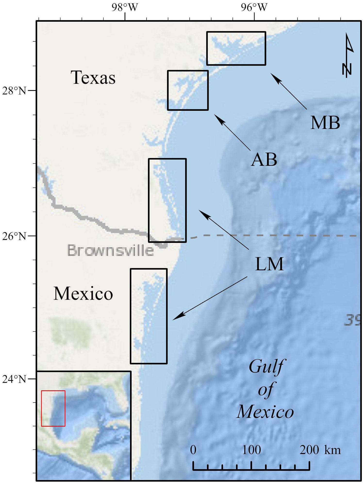
Figure 1. Northwestern Gulf of Mexico showing location of major bay systems where juvenile green turtles were collected and tracked from 2006 to 2011. These bays include: Matagorda Bay (MB), the Aransas Bay complex (AB), and the Laguna Madre (LM). The Laguna Madre in Mexico represents overwintering areas utilized by juvenile green turtles; no turtles were collected from this bay system. The dashed gray line represents the limit between the Exclusive Economic Zones of the United States and Mexico.

In-water capture was accomplished following methods outlined by Metz and Landry (2013, 2016) and consisted of daytime sets of 91.4 m long entanglement nets either 2.7 or 3.7 m deep with 12.7–17.7 cm bar mesh of #9 twisted line. Water depth dictated net type used at a particular site, but all capture effort was restricted to depths < 3 m. Netting effort at all stations consisted of 2–4 nets set in tandem or perpendicular to one another for 6–12 h per day. Net checks occurred every 20 min, or more frequently as evidence of capture dictated (e.g., surface splashes along the net line, portions of the net line no longer visible, etc.). All green turtles were photographed, measured for straight carapace length (SCL, cm), and examined for presence of flipper tags/scars and Passive Integrated Transponder (PIT) tags. Untagged individuals received an Inconel style 681 tag (issued by the NMFS SEFSC-Miami) affixed to the trailing edge of each front flipper and a PIT tag embedded under the dorsal surface of the right front flipper prior to release (Metz and Landry, 2013, 2016). Three individuals were obtained from rehabilitation centers along the Texas coast, including the NMFS Sea Turtle Facility (in conjunction with Moody Gardens Aquarium in Galveston, TX, United States), the Animal Rehabilitation Keep (ARK) in Port Aransas, TX, United States, and Sea Turtle Inc. in South Padre, TX, United States.

Transmitter Deployment and Track Data Filtering

Wild and rehabilitated turtles were equipped with platform terminal transmitter (PTT) models Kiwisat 101 and 202 (Sirtrack, Havelock North, New Zealand). Attachment followed techniques described in Seney et al. (2010). Transmitters were attached to the dorsal surface of the carapace via a two-part epoxy adhesive followed by a coat of anti-fouling paint to deter biofouling around the transmitter. To minimize stress and handling, turtles captured by entanglement net were held in plastic bins before, during, and immediately following the PTT attachment process. All wild captured individuals were released within 12 h of initial capture. Rehabilitated individuals were equipped with PTTs while housed at the rehabilitation facility after full medical clearance was granted by veterinarians. PTTs were programmed to a transmission (duty) cycle of 6 h on:6 h off.

Raw satellite track data were collected via the Argos Satellite System and processed by Argos/CLS America. Location data were paired with depth, water temperature, distance from shore, travel speed/distance traveled relative to previous location, and cumulative number of transmission hours via Service Argos. All coordinate data were processed using the least-squares algorithm and location classes (LCs) were assigned, in order of most to least accurate, as: 3 (<250 m), 2 (250 to <500 m), 1 (200 to <1,500 m), 0 (>1,500 m), A & B (Argos estimated accuracy unknown), and Z (locations failing Argos plausibility tests). Post Argos processing, data were filtered to remove questionable locations and those on land using the Satellite Tracking and Analysis Tool (STAT; Coyne and Godley, 2005). Final raw Argos track locations were further filtered based on the following criteria: (1) location codes classified as LC Z; (2) locations requiring swimming speed > 5 kph relative to the previous message; (3) locations classified at elevations > 0.5 m; or (4) points obviously on land or those with implausible pathways over land (for similar filtering methods, see also: Hart and Fujisaki, 2010; Seney and Landry, 2011; Hart et al., 2012, 2015; Coleman et al., 2017). Filtered raw coordinate data were used to reconstruct original track routes and to determine displacement from the original release location.

Behavior Analysis Using Hierarchical Switching State-Space Modeling (hSSM)

Switching state-space models utilize raw track data to determine behavioral state in a bimodal context by providing a behavioral index between 1 and 2, referred to as a “b” value. Mode 1 (e.g., “migrating”) is represented by b values < 1.5 and mode 2 (e.g., “resident/foraging”) is represented by b values > 1.5 (Jonsen et al., 2005; Breed et al., 2009). Previous studies have applied SSM to determine inter-nesting, intra-nesting, and foraging site fidelity and migratory corridors, primarily in nesting females, including Caretta caretta (Hart et al., 2012, 2013, 2015; Evans et al., 2019); Dermochelys coriacea (Bailey et al., 2008; Hoover et al., 2019); Lepidochelys kempii (Shaver et al., 2013; Coleman et al., 2017); and Lepidochelys olivacea (Maxwell et al., 2011; Dawson et al., 2017). In previous studies, results from SSM analyses performed on individual tracks are subsequently combined for estimation of core use and home range areas via additional analyses (Coleman et al., 2017; Dawson et al., 2017; Evans et al., 2019). Hierarchical SSMs (hSSM) are applied to a group of individuals in order to elucidate meaningful population-level movement data (Jonsen et al., 2006; Breed et al., 2009; Jonsen, 2016). Turtles tracked in this study originated from three geographically distinct bay systems along the Texas coast, therefore hSSM was applied to the full raw track data set to characterize population scale movements and timing of seasonal migrations.

The hSSM was run using RStudio (ver 1.1.456; R Core Team, 2019) package ‘bsam’ (Jonsen et al., 2017). Mean daily locations (timestep = 1.0) were calculated using 1,000 samples for each of two Monte-Carlo Markov Chains (MCMC) thinned by a factor of 10 from 10,000 samples following a 40,000 burn-in. Initial runs of the model used a 12-h time step (0.50) which was determined by calculating the average number of daily transmissions from the raw dataset (Maxwell et al., 2011; Dawson et al., 2017). Due to the presence of large gaps in some tracks and relatively short durations in others causing limited convergence of the model, time step was increased to 24 h for the final iteration, allowing for clear convergence of the model. This aided in reduction of erroneous points on land, improbable track pathways, and has been shown to be a sufficient duration based on previous SSM analyses using satellite tracks from juvenile sea turtles (Coleman et al., 2017). Trace plots were examined for autocorrelation and convergence on a mean density. The resulting tracks were visually inspected to validate that the model-generated tracks were biologically plausible (Dawson et al., 2017). Resulting locations estimated from hSSM were used to determine timing of migration(s), periods of residency, and core home range values.

Prior to use in further analyses, hSSM estimated locations were visually inspected and adjusted in comparison to the raw dataset. Occasionally, hSSM locations occurred on land (elevation > 0.5 m), either due to prolonged gaps in the data or inconsistent duration between raw track locations (Bailey et al., 2008; Shaver et al., 2013; Hart et al., 2015). When reasonable, locations located on land were manually moved to the closest, most probable in-water location. Locations resulting from the hSSM were compared to the raw track locations to determine if direction and geographic distribution were consistent between the two data sets. If a questionable hSSM location could not be confidently relocated, the location was discarded from further analyses (Shaver et al., 2013; Hart et al., 2015; Dawson et al., 2017). Finally, raw track data from individuals in this study showed that tracks did not occur within water > 100 m in depth. Therefore, hSSM locations resulting in > 100 m depth were removed from further analyses (Shaver and Rubio, 2008; Seney and Landry, 2011; Shaver et al., 2013). Results from hSSM were used to identify migration dates based on resulting b values. Periods of migration were defined using mean daily b values ≤ 1.5 while resident/foraging periods were defined using mean daily b values > 1.5.

Home Range and Core Area

Prior to use in home range and space-time analyses, resident/foraging locations were filtered to remove b values < 1.6 as these represent behavioral transitions from migrating to resident/foraging behaviors (Dawson et al., 2017). The remaining hSSM locations were used to determine core (50%) and home range (95%) areas via the Kernel Density Estimator (KDE) tool within the Geospatial Modeling Environment (GME) software (Beyer, 2015), the ‘ks’ library in RStudio (Duong et al., 2019; R Core Team, 2019), and ArcGIS Pro (ESRI, 2020). Point locations were projected using the Universal Transverse Mercator, Zone 14 North coordinate system. Numerous studies have analyzed the effect of smoothing parameter choice on resulting KDE (Hemson et al., 2005; Downs and Horner, 2008; Kie et al., 2010; Walter et al., 2015). Choice of smoothing parameter is more impactful on home range data than choice of kernel function as smoothing parameter has a stronger effect on estimates when compared to effects of differing kernel functions (Worton, 1989; Wand and Jones, 1995). To this end, a Smoothed Cross Validation (SCV) smoothing parameter was selected as it provided the best fit to the hSSM coordinates and has been used in previous studies (Hemson et al., 2005; Coleman et al., 2017). Cell size was set to 500 m in order to reduce pixilation of the output raster and to allow reasonable processing times, as recommended in the GME manual (Beyer, 2015). The GME ‘Isopleths’ tool was used to contour the core and home range areas. Core and home range contours were merged across all individuals to elucidate population-level habitat use patterns and distribution.

Space-Time Hot Spot Track Analyses

Hot spot analysis assesses whether high or low values of observed incidents (in this case, transmitted tag locations) are clustered spatially. It requires aggregating point observations to estimate incident intensity and then calculate the local Getis-Ord (G_i^∗) statistic for each feature; see Getis and Ord (1992) for full description of algorithm. The G_i^∗ statistic returned for each feature is a z-score. For significantly positive z-scores, the larger the z-score is, the more intense the clustering of high values (e.g., “hot spots”). For significantly negative z-scores, the smaller the z-score is, the more intense the clustering of low values (e.g., “cold-spots”). Compared to hot spot analysis, space-time analysis provides additional insights to hot or cold spot clustering as it seeks to determine when and where clustering of incidents occurs on a spatiotemporal scale. Space-time analysis includes cluster analysis and explores space-time pattern mining techniques used to analyze spatiotemporal data, identify trends, and visualize changes in patterns over time. The Mann-Kendall trend test is performed on every location with data as an independent bin time-series test. This test requires a minimum of 10 time steps and is based on the Mann–Kendall statistic, a rank correlation analysis for the bin values and their time sequence (Gilbert, 1987). The trend for each bin time series is recorded as a z-score and a p-value. The sign associated with the z-score determines if the trend is an increase in bin values (positive z-score) or a decrease in bin values (negative z-score). Consequently, eight potential trend patterns of hot spots and cold-spots can be produced if a trend pattern is detected, otherwise a “no pattern” will be reported (ESRI, 2020). This spatiotemporal analytic has only recently been applied in an ecological context and it is applied in this study to analyze the movement of green turtles and their habitat use (Bevanda, 2015).

Due to a large data gap between consecutive years of the study (i.e., no location data generated from September 2007 to August 2009), filtered hSSM resident/foraging locations for migratory individuals were aggregated into monthly time steps representing temporal partitions from December through November. December was selected as the starting time step for two reasons: (1) this coincides with the beginning of the “winter” season (Coleman et al., 2017) and (2) it is the earliest month in which any migratory individual exhibited an initial migration out of Texas waters. A hexagonal space-time cube was created by aggregating point locations into bins of 3 km spatial resolution and 1 month time step. A 3 km spatial resolution was selected for consistency with the precision of the telemetry LCs (average ∼1.5 km radius). This space-time cube was then incorporated with a fixed distance “neighborhood” in order to assess local space-time clustering and hot spot trends following the Mann–Kendall trend test. A 10 km “neighborhood” was selected based on the average width of core areas generated from the KDE analyses. Space-time hot and cold spots were visualized in 3D rendering based on the structure of the created space-time cube.

Habitat Association: Seagrass and Water Temperature

Green turtle habitat use was assessed by examining the relationship between turtle locations and: (1) seagrass habitat (area and % coverage); and (2) water temperature. Seagrass coverage data was obtained from the National Oceanic and Atmospheric Administration (NOAA, 2019) and includes aquatic vascular vegetation beds dominated by submerged, rooted, vascular species or submerged or rooted floating freshwater tidal vascular vegetation for Texas waters only. The KDE core home range areas were analyzed spatially to quantify overlap of seagrass areas for each individual. Mean daily latitudes of migratory individuals were plotted against Argos-satellite-derived SST associated with PTT-derived raw locations to determine temperature range in which turtles were exposed along their tracks. Data provided by the National Data Buoy Center (NDBC; NOAA, 2020) was used to compare water temperatures in the bay versus hSSM-derived daily latitude. Data provided by the NDBC is generated every 6 min, but the hSSM generates a mean daily location with a model derived time stamp. In order to compare mean daily location with daily SST in the original bay of capture, only buoy water temperature readings closest to 20:00 UTC (±1 h) were used.

Statistical Analyses

Descriptive statistics and statistical analyses were performed using a combination of Microsoft Excel 2016 and SigmaPlot 14.0. All data are reported as mean ± one standard error (SE), unless otherwise noted, and statistical significance was α = 0.05. Comparisons of SCL, hSSM derived durations of residence, and raw track duration were assessed using one-way ANOVA in order to detect significant differences between bay systems and seasonal residencies. Kruskal–Wallis one-way ANOVAs on Ranks was used to compare PTT associated displacement for each location versus the original release location. A one-way ANOVA was performed to detect significant differences in buoy water temperatures within the bay of origin during green turtle residency and migratory periods. A non-linear regression analysis of buoy-derived daily SST and hSSM-generated latitudes was performed to ascertain the temperature at which green turtles begin an initial migratory phase. A Kruskal–Wallis one-way ANOVA on Ranks was used to compare the amount of overlap of seagrass bed density and KDE 50% and 95% contours between estuaries in which each individual was originally captured. For all one-way ANOVA and Kruskal–Wallis one-way ANOVA on Ranks, pairwise comparisons were made using the Holm–Sidak or Dunn’s method, respectively.

Results

Satellite Telemetry and Track Analyses

Raw Track Data

Between June 2006 and April 2011, fifteen wild (n = 12) and rehabilitated (n = 3) juvenile green sea turtles were fitted with PTT transmitters and tracked via satellite telemetry. Overall mean SCL of tracked turtles was 53.1 ± 2.42 cm (range: 40.0–69.2 cm) (Supplementary Table S1). Track duration ranged from 16 to 344 days (mean: 129 ± 24.4 days) for a combined total of 1,929 tracking days. No significant differences were detected between rehabilitated and wild individuals for SCL (F₁,₁₃ = 0.0124, p = 0.913) or track duration (F₁,₁₃ = 0.0114, p = 0.917). Additionally, no significant differences were detected between bay systems for SCL (F₂,₁₂ = 0.589, p = 0.570) or track duration (F₂,₁₂ = 1.179, p = 0.341). Track locations ranged between 29°N and 23°N, and 96°W and 98°W (Supplementary Figure S1). After filtering via Argos and STAT, raw track data produced 1,993 locations with individual tracks ranging from 34 to 511 locations (mean: 133 ± 33 locations). The majority of LC were classified as A and B (n = 455 and 910, respectively) while LCs 0–3 comprised the remaining 31.5% of locations. Individual track notes are provided in Supplementary Table S2.

hSSM Track Data

Total number of mean daily locations generated by hSSM was 1,924, forty of which (2.1%) were excluded from analyses due to depth, occurrence on land, or questionable location. Two-hundred and fifty-four (13.2%) locations were reliably relocated based on comparison to raw track data. Of the remaining locations, 1,799 (95.5%) were assigned b values > 1.5 (foraging/resident) while 85 (4.5%) were assigned b values < 1.5 (migrating). All coordinates from May to November were classified as b > 1.5 (foraging/resident) and were restricted to nearshore and inland waters of Texas (Figure 2). No significant differences were detected in days spent in summer residency between rehabilitated and wild turtles (F₁,₁₃ = 0.0027, p = 0.960) or between the bay system each turtle originated from (F₂,₁₂ = 0.306, p = 0.742). During summer residencies, mean displacement from release location for all turtles (based on raw track data) was 12.9 ± 0.60 km (maximum = 182.2 km, n = 1,673). One turtle exhibited movements outside of its bay of origin during summer residency. When excluded from displacement analyses, the mean displacement of the remaining 14 tracks declined to 9.7 ± 0.3 km (maximum = 94.2 km, n = 1,598).

FIGURE 2

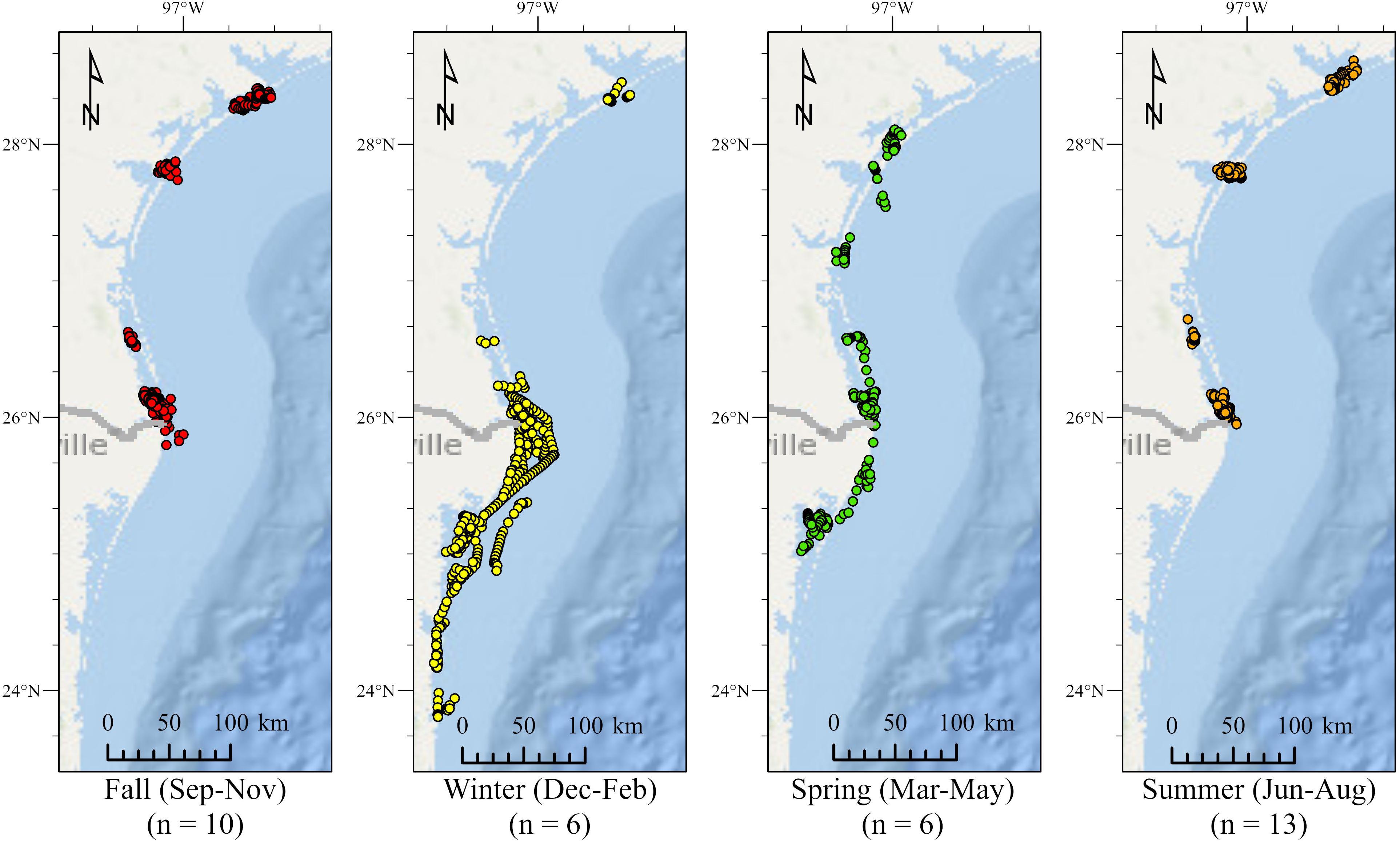
Figure 2. Hierarchical switching state-space model (hSSM) mean seasonal daily locations of juvenile green turtles tracked in the northwestern Gulf of Mexico (N = 15). Number of individuals tracked each season indicated below season headers. Fall (red) and summer (orange) locations were restricted to inland waters within Texas bays and estuaries. Winter (yellow) locations showed longest migrations in to the Laguna Madre in Mexico. Spring (green) locations were not as widely distributed as winter locations, but extended into Mexican waters.

Five turtles (all originating from the Laguna Madre) exhibited migrations based on hSSM analysis (Figure 3). Winter residencies for all migratory turtles were significantly shorter than summer (F₁,₈ = 5.710, p = 0.044), though no significant differences were detected in number of days spent migrating between season (F₁,₈ = 0.132, p = 0.911). Almost half of all migrations occurred in January and March (20.0% and 28.2%, respectively), though turtles exhibited migratory behavior every month from December to April (Figure 2). The earliest winter migration was detected on December 4th with the latest summer return to residency in Texas occurring on April 27th. During winter months, all migratory individuals were restricted to waters of the Laguna Madre in Texas and Mexico. From these five tracks, two distinct migration patterns were observed: (1) a meandering, “indirect” migration with multiple punctuated intervals of foraging/residency and migration prior to establishing a clear residence location and (2) a clear, “direct” migration with large distances traveled over short periods and quickly established residency (Figure 3).

FIGURE 3

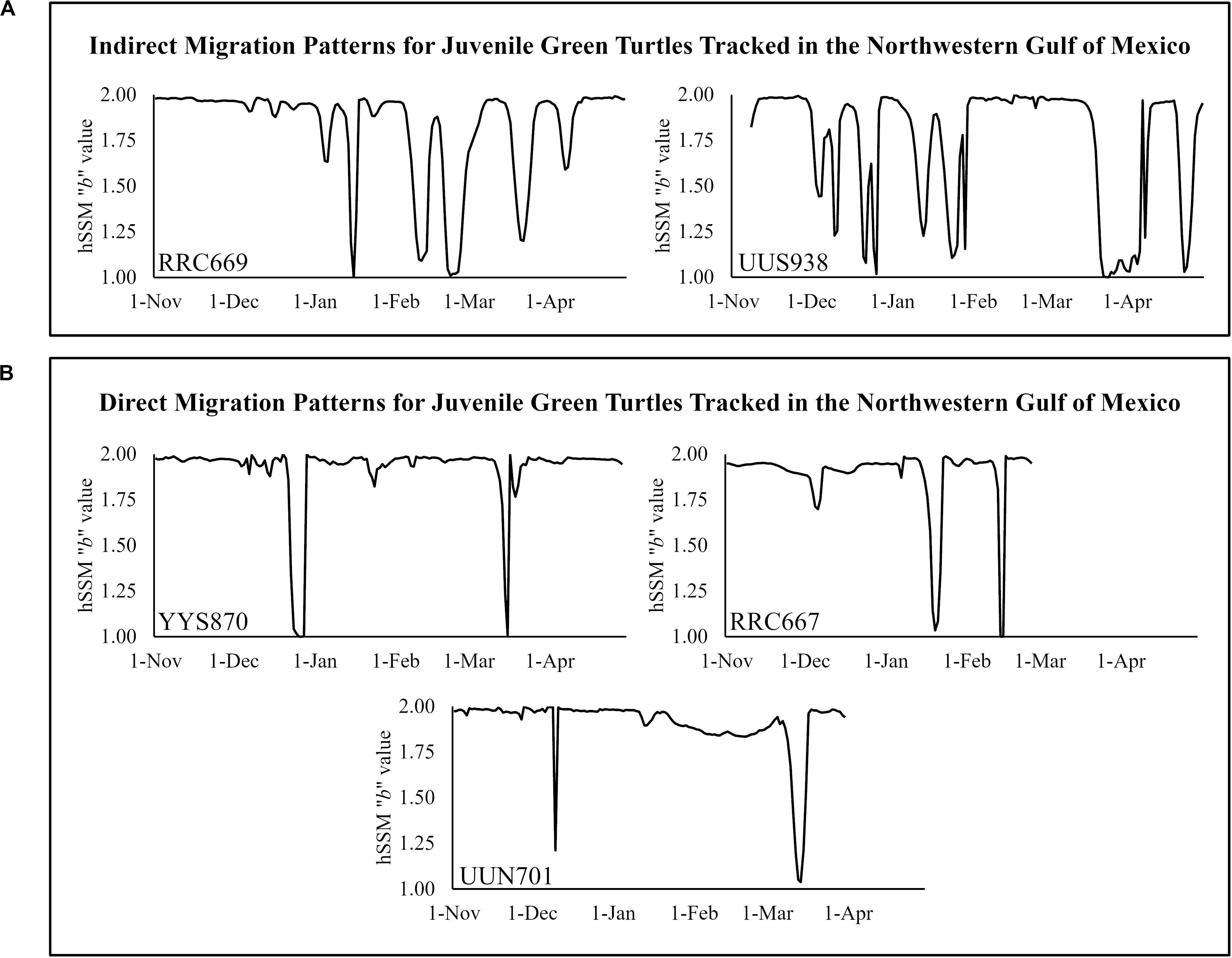
Figure 3. Migration patterns for juvenile green turtles satellite tracked in the northwestern Gulf of Mexico (n = 5). hSSM “b” values >1.5 are representative of foraging/residency behavior, while values <1.5 are representative of migratory behavior. (A) “Indirect” migratory pattern characterized by multiple alternations between migration and short-term residency prior to establishment of overwintering residency in Mexican waters. (B) “Direct” migratory pattern characterized by unidirectional short migration period and prolonged overwintering residency prior to summer remigration back to United States waters.

KDE and Space-Time Hot Spot Analyses

KDE

Prior to use in KDE and Space-Time analyses, 10 (0.5%) transitional b values (<1.6) were removed from the 1,799 hSSM foraging/resident b values. Mean summer core and home range areas were 125.4 ± 47.5 km² and 543.7 ± 230.6 km², respectively, while mean winter core and home range areas were 274.4 ± 525.9 km² and 3,266.8 ± 1,537.3 km², respectively. No significant differences were detected in size of winter (e.g., Mexico) versus summer (e.g., Texas) core areas (H = 1.009, df = 1, p = 0.315) though winter 95% contours were significantly larger than summer (H = 8.550, df = 1, p = 0.003) (Supplementary Table S1). Turtle UUS938 exhibited longer migrations than the other four individuals and was the only turtle that did not remain in its bay of origin during summer residencies. Mean summer core and home range contours with UUS938’s track excluded were 93.4 ± 37.7 km² and 334.9 ± 104.9 km², respectively, while mean winter core and home range areas were 22.0 ± 20.1 km² and 1,755.5 ± 363.6 km², respectively. Total 50% KDE area (including UUS938) between Texas and Mexico was 2,708 km² while 95% contours encompassed 10,826 km² (Figure 4).

FIGURE 4

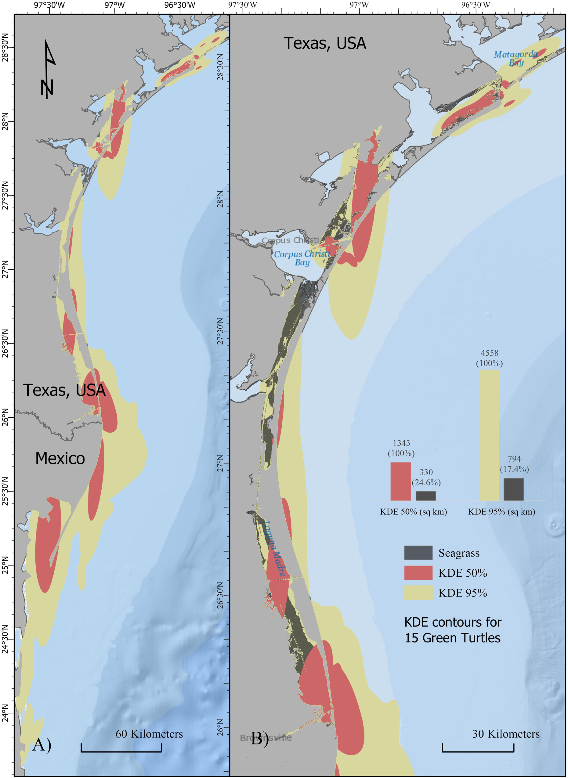
Figure 4. Map of 50% (red) and 95% (yellow) KDE contours for juvenile green turtles satellite tracked in the northwestern Gulf of Mexico (N = 15). (A) 50% and 95% contours for entire sample area, including winter residencies in Mexico. (B) 50% and 95% contours overlaid with seagrass bed locations (gray) in Texas (data not available for Mexico).

Space-Time Hot Spot Analysis

No Cold Spot trends were detected throughout the study area. Consecutive and Sporadic Hot Spot trends were detected over time in the lower reaches of the Laguna Madre near Port Isabel, TX (Figures 5A,B). Consecutive Hot Spot trends represent locations with a single uninterrupted run of statistically significant hot spot bins occurring in the final time step intervals. Sporadic Hot Spot trends represent areas of “on-again, off-again” hot spots where less than 90% of time step intervals are statistically significant and none of the time step intervals are identified as cold spots. A New Hot Spot trend over time was detected in the upper reaches of the Laguna Madre near Port Mansfield, TX, United States (Figure 5C). New Hot Spot trends represent locations where statistically significant hot spots occur in the final time step (November) and has not previously represented a significant hot spot (Bevanda, 2015; ESRI, 2020). During individual time steps (Figure 5D), hot spot areas were detected across all months, but not always during consecutive months. Increased occurrence of hot spots in southern latitudes tended to occur in earlier months (January–March), while increased occurrence of hot spots in northern latitudes tended to occur later in the year (April–December). Hot spots in northern estuaries (Matagorda Bay and Aransas Bay) were identified in May and June, only.

FIGURE 5

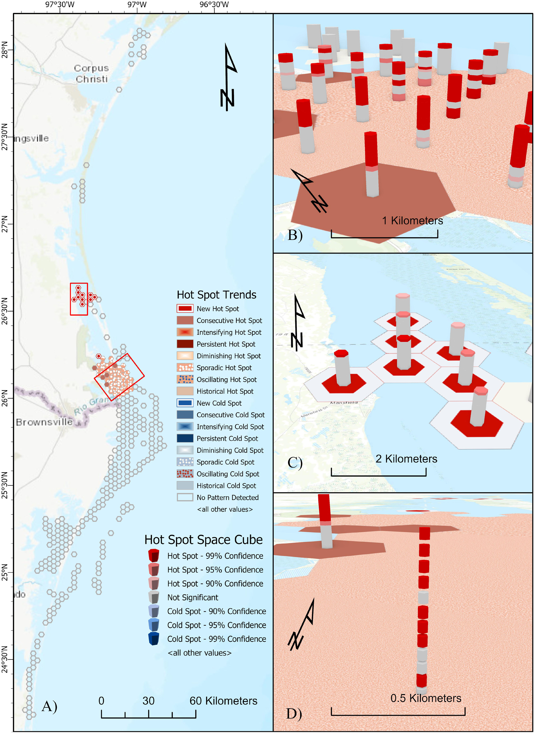
Figure 5. Space-time hot spot analysis results using mean daily location from hSSM for juvenile green turtles tracked in the northwestern Gulf of Mexico (N = 15). (A) 2D mapping of the hot spot trend analysis showing Consecutive and Sporadic hot spot trends in the lower reaches of the Laguna Madre and New hot spot trends in the upper reaches of the Laguna Madre (red boxes). (B) 3D visualization of the Consecutive and Sporadic hot spot trends in the lower Laguna Madre. (C) 3D visualization of New hot spot trends in the upper Laguna Madre. (D) A closer look at the Sporadic hot spot trend area of the lower Laguna Madre showing changes in hot spots over time. Monthly time step bins represented by vertically stacked cubes (December = bottom of stack; November = top of stack). Periods of hot spot activity indicated by red cubes.

Habitat Association: Seagrass and Water Temperature

Seagrass

Of the available 907 km² of seagrass bed found within Texas bays, 87.5% (794 km²) fell within the 95% KDE contours. Seagrass beds comprised 24.6% (330 of 1,343 km²) of the core area and 17.4% (794 of 4,558 km²) of the home range (Figure 4). Seagrass was least prevalent within the core area for turtles originally captured in Aransas Bay and most abundant in core areas of turtles originally captured in the Laguna Madre (H = 6.060, df = 2, p = 0.048). Core areas of turtles originally captured in Matagorda Bay did not contain significantly different seagrass coverage within their core area when compared to turtles originating from either the Laguna Madre or Aransas Bay. No significant differences were detected between original capture location and amount of seagrass present within the 95% home range (H = 4.031, df = 2, p = 0.133).

Water Temperature

All migratory individuals (n = 5) originated from the Laguna Madre, therefore water temperature analyses were confined to this estuary. When plotting Argos-satellite-derived SST against mean daily latitude from the PTT-derived location data, all individuals remained in areas where water temperatures were above 15°C, regardless of latitude (Figure 6A). Water temperature data from the NDBC was obtained from buoy station PTIT2 (26.061°; −97.215°) near Port Isabel, Texas. A significant difference in mean NDBC-derived water temperature was detected between summer (24.7°C ± 0.16, range: 11.6–36.3°C) and winter (16.1°C ± 0.15, range: 10.3–21.3°C) residencies (F₁,₉₃₀ = 870.3, p < 0.001). Mean water temperature in the Laguna Madre was 15.9°C ± 0.58 (range: 11.6–20.5°C) at onset of the initial migration. Mean latitude at which migration was first detected was 25.7°N ± 0.08 (range: 24.9°N–26.1°N). Regression analysis of hSSM-derived latitudes versus NDBC-derived water temperature revealed a non-linear relationship where turtles initiated migration to lower latitudes as water temperatures declined in the Laguna Madre (r² = 0.4917, df = 1135, p < 0.001) (Figure 6B). The intersection between this regression line and the mean latitude during the initial migratory period (25.7°N, red dotted line) coincides with a water temperature near 19°C (red solid line).

FIGURE 6

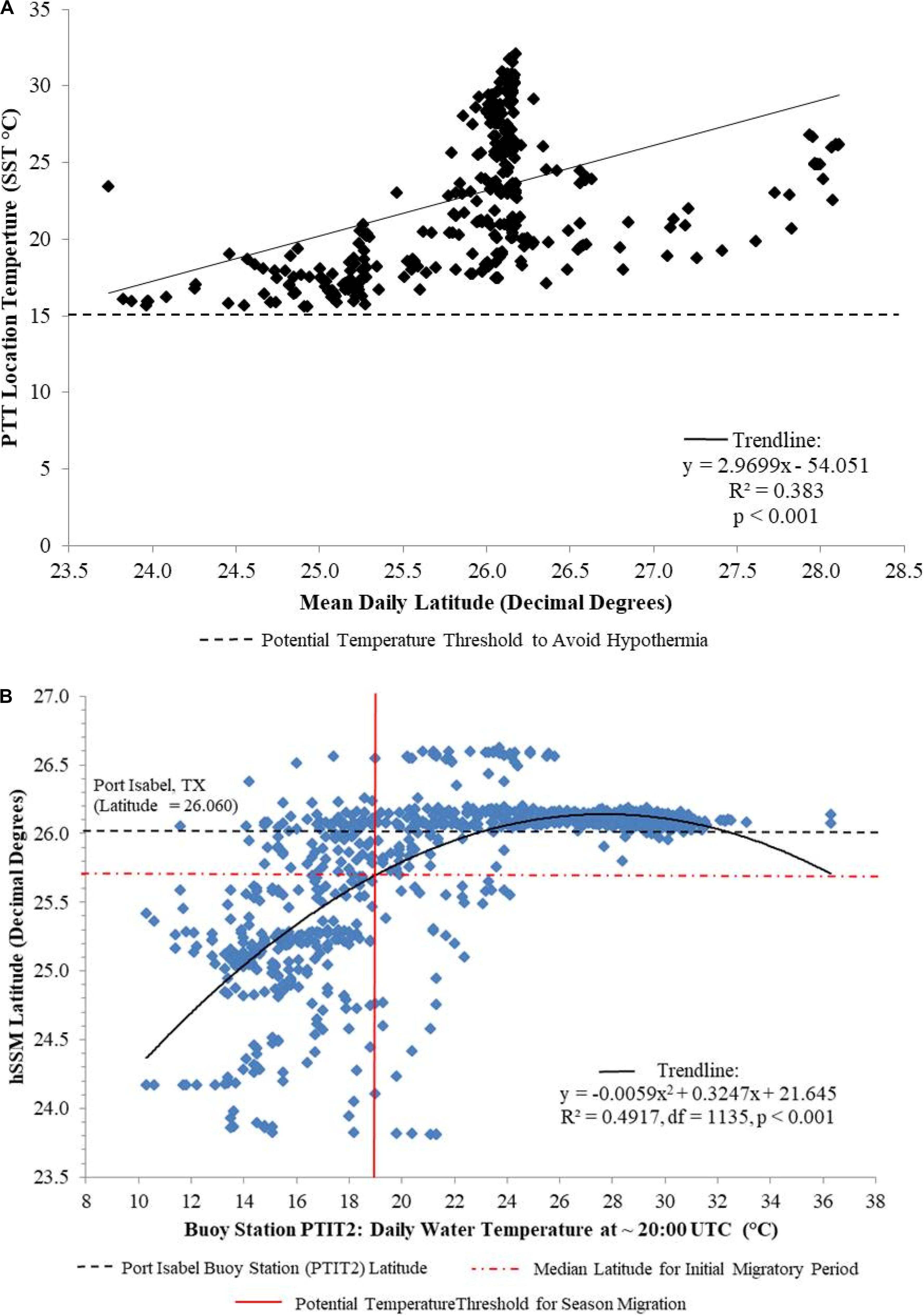
Figure 6. Water temperature associations for juvenile green turtles satellite tracked in the northwestern Gulf of Mexico (n = 5). (A) Mean daily latitude from raw track data versus satellite tag sea surface temperature (SST). All turtles remained within waters > 15°C (horizontal dashed line). (B) Mean daily buoy temperature at Port Isabel, TX, United States (latitude = black dashed line) versus mean daily latitude from hSSM data. The intersection between this trend line (solid black line) and mean latitude during the initial migratory period (25.7°N, red dotted line) coincides with a water temperature near 19°C (red solid line).

Discussion

Green turtles tracked in this study displayed strong seasonal fidelity to their original capture locations. Turtles remained in nearshore waters < 10 m depth with mean displacement < 13 km during summer months, similar to other studies (Ogden et al., 1983; Seminoff et al., 2002; Hart and Fujisaki, 2010; Vélez-Rubio et al., 2018; Wildermann et al., 2019). However, the size of core areas utilized by greens in this study were larger, overall wider-ranging (range: 3.0–1,284.0 km²; Supplementary Table S1; Figure 4), and varied seasonally (summer: 125.4 ± 47.5 km², n = 15; winter: 274.4 ± 252.9 km², n = 5) as compared to other tracking studies from the Gulf of Mexico. Smaller core use areas have been observed for juvenile green turtles tracked in the northeastern Gulf of Mexico, though it should be noted that these turtles were tracked via differing methods (Hart and Fujisaki, 2010 = 5.0–54.5 km²; Lamont et al., 2015 = 1.056 ± 2.540 km²; Lamont and Iverson, 2018 = 4.8 ± 5.2 km²; Wildermann et al., 2019 = 4.4 ± 1.3 km²). Conversely, juvenile green turtles undertaking seasonal migrations in the southwestern Atlantic exhibit larger core areas when foraging (1,176–4,987 km²; González Carman et al., 2012). Differences in the size of core use areas among these studies may be attributed to various factors including track duration, tracking methodology (i.e., radio vs. sonic vs. acoustic vs. satellite telemetry), turtle size, regional population variability, seasonal movements, and differing environmental conditions. This suggests that more information is needed to understand the factors driving variability in habitat utilization and size of foraging area in the greater Atlantic basin.

Only 4.5% of hSSM locations identified in this study were classified as migratory (b < 1.5), supporting observations of short periods of migratory behavior from previous studies (Maxwell et al., 2011; Hart et al., 2012, 2013; Coleman et al., 2017; Dawson et al., 2017; Evans et al., 2019). Turtles exhibited resident/foraging behavior for the majority of their track durations, including the overwintering period in Mexico. Core areas were not significantly different between summer and winter residencies, though 95% contours were significantly larger in winter, suggesting that individuals may be more mobile during this time. This increase in 95% contours during winter residencies may be attributed to bathymetry of the Mexican coast with narrower shelves, deeper bays, and deeper drop offs near passes and bay inlets/outlets. As turtles search for foraging areas, they may be required to travel greater distances in order to find suitable habitat. Core area contours encompass the full coastline in the Laguna Madre of Texas and Mexico (Figure 4), including migratory pathways, suggesting that this entire coastline may be critical habitat for the population. Migrations were detected from December-April, though nearly half occurred in January and March (20.0% and 28.2%, respectively; Figure 2). Variation in migration occurrence around these 2 months may likely be attributed to annual environmental variability and should be evaluated further in future studies. Our results suggest that areas along the United States and Mexico border represent essential habitat for juvenile green turtles in the northwestern Gulf of Mexico.

For the majority of tracks exhibiting migrations, these migrations were “direct” and occurred over short periods (n = 3). Some tracks exhibited multiple short residence-migration alternations before settling in their final overwintering location, sometimes weeks after instigating their initial migration (n = 2). Though sample size is small in this study, clear differences in track types were observed (Figure 3). These types of migration patterns have been observed previously with adult nesting loggerhead and Kemp’s ridley turtles (Shaver, 1991; Shaver et al., 2013; Evans et al., 2019). Terms such as “opportunistic” and “indirect” have been applied to these types of tracks, where individuals make multiple short migrations with prolonged intervals of residency/foraging. In the context of this study, the term “indirect” is most appropriate to describe juvenile sea turtles exhibiting this type of migration. “Opportunistic” may have connotations with specific behaviors related to activities (e.g., foraging), though more data is necessary to draw conclusions on influences to these movement patterns. Future studies should take these types of migration behaviors into consideration when analyzing track data, especially for juveniles of populations showing migrations to short-term resident/foraging areas.

Space-time analysis assesses whether animal locations are clustered spatially and detects trends in these clusters over time. For sea turtles, space-time analysis may lend itself most useful when applied to long-term datasets for nesting females and impacts of anthropogenic and environmental alterations to nesting beaches, as well as numerous other applications. For example, areas of hot spot clustering at nesting beaches have been documented across numerous sea turtle species (Foley et al., 2013; Baudouin et al., 2015; Dawson et al., 2017; Dalleau et al., 2019; Evans et al., 2019). Hot spot analysis identifies these areas as locations of peak activity, but space-time analysis allows for resource and conservation managers to identify specific timing of these events in relation to their location. In the context of this study, space-time analysis was not used to evaluate species abundance because such investigation requires large location datasets with a large number of individuals (ESRI, 2020). Rather, the focus in this study is on better understanding the movement of migratory juvenile green turtles over time and their utilization of coastal habitats. Our analysis shows that areas of the Laguna Madre at the border of the United States and Mexico represent hot spot areas of activities, but that these hot spots are not present year-round. Consecutive hot spot trends in the Laguna Madre correspond to summer/fall residence periods and overlap locations of extensive seagrass beds. These trends are likely indicative of greater habitat quality or accessibility to seagrass beds for foraging during this time frame. Sporadic hot spot trends occur in the transitional waters between Texas and Mexico along areas where all migratory individuals passed during migrations. The timing and location of hot spots within this sporadic trend coincide with the timing of winter (December–January) and summer (March–April) migrations, as confirmed by hSSM. New hot spot trends can aid in identification of areas to increase monitoring efforts to determine if trends are constant, or occur due to anomalous events. For example, in this study, the New hot spot trends identified in the Port Mansfield area of the Laguna Madre are likely due to an artifact of release time for one individual (UUS938) and may not be indicative of hot spot area(s) for the full population. Resources managers can use the timing and location of these hot spots to coordinate timing of closures or restrict access in order to avoid habitat destruction or potential for injury to turtles within these areas.

The association of green turtles with seagrasses is expected given their herbivorous diet and documented use of nearshore waters as developmental foraging grounds (Coyne, 1994; Shaver, 1994; Renaud et al., 1995; Arms, 1996; Bjorndal, 1997; Metz and Landry, 2013). All individuals tracked in this study were > 30 cm SCL and are representative of a size class likely to forage in seagrass beds (Coyne, 1994; Metz and Landry, 2013). Although overlap of green turtle core and home range areas with seagrass coverage were 24% and 17%, respectively, 87.5% of the available seagrass habitat in Texas falls within the home range area supporting evidence for the importance of this habitat to foraging success (Figure 4). In 2006, the State of Texas designated the Redfish Bay State Scientific Area in Aransas Bay as a “prop up” zone to prevent scarring of seagrass beds (TPWD, 2020). Due to a significant reduction in prop scarring after this designation, the Texas Legislature passed HB 3279 making it illegal to uproot seagrasses coast-wide (Texas Legislature, 2013). Protecting juvenile green turtle foraging habitat may also benefit conservation and management other threatened and endangered sea turtle species. Overlap of developmental foraging habitat between green, loggerhead, and Kemp’s ridley sea turtles has been observed at other foraging areas in the northern Gulf of Mexico (Lamont and Iverson, 2018; Wildermann et al., 2019) and may be the case in Matagorda Bay, Texas where green turtles and Kemp’s ridleys are both captured in netting surveys (Metz and Landry, 2013; 2016). Given the anthropogenic threats to seagrass habitat in this region, the results of the current study support the need for continued protection of seagrass areas along the northwest Gulf of Mexico coast, especially in light of the exponentially growing green turtle population (Metz and Landry, 2013; Shaver et al., 2017).

All turtles tracked over winter in the current study migrated to and remained within waters > 15°C (Figure 6). Similar behavioral observations have been made in the southwestern Atlantic with juvenile green turtles following 20°C isobaths along Argentina and Uruguay during seasonal migrations to northern latitudes (González Carman et al., 2012). Kemp’s ridley sea turtles have been shown to reduce food consumption by 50% when water temperature is reduced from 26°C to 20°C, with immature green turtles demonstrating a similar reduction in food intake at 15°C (Moon et al., 1997). At temperatures below 15°C, both species ceased feeding and reduced swimming activity was observed in green turtles at temperatures below 20°C. The results of the current study suggest a threshold temperature near 19°C for initiating migration which is similar to other migratory aquatic megafauna. Atlantic sharpnose sharks (Rhizoprionodon terraenovae) along the northern Gulf of Mexico appear inshore in spring when water temperatures approach 20–22°C and begin to move out of the area in fall at 22–24°C (Parsons and Hoffmayer, 2005). However, the degree of temperature change within a certain timeframe may be more influential on initiating migratory behavior rather than a specific threshold temperature. Juvenile blacktip sharks (Carcharhinus limbatus) in nearshore waters of the Gulf of Mexico appear to respond to decreases in water temperature of 5°C over a 2-day period as a cue to leave their summer nursery area to avoid lethal winter temperatures (Heupel, 2007). The effect of the rate of temperature change on the migratory behavior of sea turtles should be examined in future studies.

Although cold-stunning events suggest a large portion of green turtles overwinter in Texas inshore waters (Shaver et al., 2017), results of the current study demonstrate that some green turtles are capable of making seasonal migrations in response to declining water temperatures. Seasonal migration minimizes the risk of hypothermic stunning and facilitates continued activities as temperatures in northern waters become physiologically unfavorable (Shaver et al., 2017). This behavioral response may confer a biological advantage to turtles that leave northern waters during winter months due to their ability to maintain foraging behavior. The ability to continue foraging over winter may offset the energetic cost of migration while reducing the risk of exposure to lethal water temperatures (<8°C; Shaver et al., 2017). The factors contributing to overwintering versus migratory behavior should be examined in future studies.

Overall, the results of this study have increased our knowledge of seasonal patterns in habitat use and migration of green turtles in the northwestern Gulf of Mexico. Additionally, the seasonal migration of green turtles from Texas into Mexican near coastal waters necessitates bi-national cooperation between the United States and Mexican natural resource management agencies to ensure the continued recovery of these green turtle populations. The use of novel approaches to understanding sea turtle habitat use, such as hierarchical switching state-space modeling and the use of space-time hot spot analyses as employed in our study, should be pursued to increase our knowledge of critical habitat needs of green turtles to support the development of best management strategies including the identification, designation, and conservation of critical habitat.

Conclusion

• More information is needed to understand the factors driving variability in habitat utilization and size of foraging area in the greater Atlantic basin.

• Areas along the United States and Mexico border represent essential habitat for juvenile green turtles in the northwestern Gulf of Mexico.

• Future studies should take migratory patterns (indirect vs. direct) into consideration when analyzing track data, especially for juveniles of populations showing migrations to short-term resident/foraging areas.

• Resources managers should utilize timing and location of space-time hot spots when making management decisions for migratory species.

• The results of the current study support the need for continued protection of seagrass areas along the northwest Gulf of Mexico coast, especially in light of the exponentially growing green turtle population.

• The effect of the rate of temperature change on the migratory behavior of sea turtles should be examined in future studies.

• The factors contributing to overwintering versus migratory behavior should be examined in future studies.

Data Availability Statement

The datasets generated for this study are available on request to the corresponding author.

Ethics Statement

The animal study was reviewed and approved by Institute for Animal Care and Use Committee – Texas A&M University (AUP 2009-27).

Author Contributions

TM served as the field coordinator for this study, conducted entanglement netting surveys, satellite transmitter deployment, and performed analyses examining habitat associations. MG assisted with netting surveys, satellite transmitter deployment, and performed analyses related to hSSM, KDE, and statistics. MM assisted with all GIS analyses, including KDE and space-time hot spot analyses. GG provided resources for all analyses and consulted on all environmental and habitat association analyses. All authors contributed to final manuscript documents and materials including manuscript, table, and figures development.

Funding

Funding for this research was made available by the Texas Sea Grant Program, Sea Turtle Restoration Project, and Texas Parks and Wildlife Department (TPWD) Kills and Spills Team (KAST) Restitution fund.

Conflict of Interest

The authors declare that the research was conducted in the absence of any commercial or financial relationships that could be construed as a potential conflict of interest.

Acknowledgments

Authorization for sea turtle capture and data collection was granted under NMFS Permit Numbers 1526, 1526-02, and 15606 and TPWD Scientific Permit Number SPR-0590-094. We would like to thank the director of the Sea Turtle and Fisheries Ecology Research Lab, Dr. Andre M. Landry, Jr., and field crew members in our sea turtle netting program for their hard work and dedication, with special recognition given to Michelle Puig, Tracy Weatherall, Katie St. Clair, and Darrin Dukes for their multiple years of contribution. Additional thanks go to the Marine Biology Department (with special thanks to Stacie Arms) and Research and Graduate Studies Offices at Texas A&M University at Galveston, Texas Parks and Wildlife Department, U.S. Coast Guard, Tony Amos of the Animal Rehabilitation Keep at the University of Texas Marine Science Institute, Ben Higgins of the NMFS Galveston Sea Turtle Facility, Greg Whitaker and Roy Drinnen of Moody Gardens Aquarium, Dr. Joe Flanagan of the Houston Zoo, Jeff George of Sea Turtle, Inc., Dr. Tom DeMaar, Dr. Tim Tristan, Mr. and Mrs. J. D. Whitley of Port Mansfield, TX, United States, Dr. Donna Shaver of Padre Island National Seashore, and the U.S. Army Corps of Engineers Galveston District for providing various means of support from administrative assistance and data contributions to facilities for our operations and housing of personnel and turtles while in the field. We would also like to thank Carole Allen, former Director of the Gulf Office of the Sea Turtle Restoration Project, for providing funds for this research during the 2008 season.

Supplementary Material

The Supplementary Material for this article can be found online at: https://www.frontiersin.org/articles/10.3389/fmars.2020.00647/full#supplementary-material

FIGURE S1 | Raw track locations for juvenile green turtles tracked in the northwestern Gulf of Mexico (N = 15). Supplemental raw track data (dates, number of days, etc.) can be found in Supplementary Table S1. Tracks are presented as a color gradient with release dates in dark green and final tracking dates in red.

References

Arms, S. A. (1996). Overwintering Behavior and Movement of Immature Green Sea Turtles in South Texas Waters. Master’s thesis, Texas A&M University, Galveston, TX.

Google Scholar

Bailey, H., Shillinger, G., Palacios, D. M., Bograd, S. J., Spotila, J. R., Paladino, F. V., et al. (2008). Identifying and comparing phases of movement by leatherback turtles using state-space models. J. Exp. Mar. Biol. Ecol. 356, 128–135. doi: 10.1016/j.jembe.2007.12.020

CrossRef Full Text | Google Scholar

Baudouin, M., De Thoisy, B., Chambault, P., Berzins, R., Entraygues, M., Kelle, L., et al. (2015). Identification of key marine areas for conservation based on satellite tracking of post-nesting migrating green turtles (Chelonia mydas). Biol. Conserv. 184, 36–41. doi: 10.1016/j.biocon.2014.12.021

CrossRef Full Text | Google Scholar

Bevanda, M. (2015). Animals in Space and Time: Spatiotemporal Movement Pattern Analysis. Dissertation, University of Beyreuth, Bayreuth.

Google Scholar

Beyer, H. L. (2015). Geospatial Modelling Environment (Version 0.7.4.0).

Google Scholar

Bjorndal, K. A. (1997). “Foraging ecology and nutrition of sea turtles,” in The Biology of Sea Turtles, eds P. L. Lutz and J. A. Musick (Boca Raton, FL: CRC Press, Inc), 199–232.

Google Scholar

Bradshaw, P., Broderick, A. C., Carreras, C., Inger, R., Fuller, W., Snape, R., et al. (2017). Satellite tracking and stable isotope analysis highlight differential recruitment among foraging areas in green turtles. Mar. Ecol. Prog. Ser. 582, 201–214. doi: 10.3354/meps12297

CrossRef Full Text | Google Scholar

Breed, G. A., Jonsen, I., Myers, R., Bowen, W., and Leonard, M. (2009). Sex-specific, seasonal foraging tactics of adult grey seals (Halichoerus grypus) revealed by state-space analysis. Ecology 90, 3209–3221. doi: 10.1890/07-1483.1

CrossRef Full Text | Google Scholar

Chainey, S., Tompson, L., and Uhlig, S. (2008). The utility of hotspot mapping for predicting spatial patterns of crime. Secur. J. 21, 4–28. doi: 10.1057/palgrave.sj.8350066

CrossRef Full Text | Google Scholar

Coleman, A., Pitchford, J., Bailey, H., and Solangi, M. (2017). Seasonal movements of immature Kemp’s ridley sea turtles (Lepidochelys kempii) in the northern gulf of Mexico: immature Kemp’s ridley movements in Northern Gulf of Mexico. Aquat. Conserv. 27, 253–267. doi: 10.1002/aqc.2656

CrossRef Full Text | Google Scholar

Coyne, M. (1994). Feeding Ecology of Subadult Green Sea Turtles in South Texas Waters. Master’s thesis, Texas A&M University, College Station, TX.

Google Scholar

Coyne, M., and Godley, B. (2005). Satellite tracking and analysis tool (STAT): an integrated system for archiving, analyzing and mapping animal tracking data. Mar. Ecol. Prog. Ser. 127, 1–7. doi: 10.3354/meps301001

CrossRef Full Text | Google Scholar

Crowder, L. B., Crouse, D. T., Heppell, S. S., and Martin, T. H. (1994). Predicting the impact of turtle excluder devices on loggerhead sea turtle populations. Ecol. Appl. 4, 437–445. doi: 10.2307/1941948

CrossRef Full Text | Google Scholar

Dalleau, M., Kramer-Schadt, S., Gangat, Y., Bourjea, J., Lajoie, G., and Grimm, V. (2019). Modeling the emergence of migratory corridors and foraging hot spots of the green sea turtle. Ecol. Evol. 9, 10317–10342. doi: 10.1002/ece3.5552

PubMed Abstract | CrossRef Full Text | Google Scholar

Dawson, T. M., Formia, A., Agamboué, P. D., Asseko, G. M., Boussamba, F., Cardiec, F., et al. (2017). Informing marine protected area designation and management for nesting olive ridley sea turtles using satellite tracking. Front. Mar. Sci. 4:312. doi: 10.3389/fmars.2017.00312

CrossRef Full Text | Google Scholar

Downs, J. A., and Horner, M. W. (2008). Effects of point pattern shape on home-range estimates. J. Wildlife Manage. 72, 1813–1818. doi: 10.2193/2007-454

CrossRef Full Text | Google Scholar

Duong, T., Wand, M., Chacon, J., and Gramacki, A. (2019). Kernel Smoothing. RStudio Package ‘ks’ Version 1.11.7. Available online at: https://cran.r-project.org/web/packages/ks/index.html (accessed February 28, 2020).

Google Scholar

Dutton, P. H., Leroux, R. A., Lacasella, E. L., Seminoff, J. A., Eguchi, T., and Dutton, D. L. (2019). Genetic analysis and satellite tracking reveal origin of the green turtles in San Diego Bay. Mar. Biol. 166:3.

Google Scholar

ESRI (2020). ArcGIS Pro. Redlands, CA: Environmental Systems Research Institute.

Google Scholar

Evans, D. R., Carthy, R. R., and Ceriani, S. A. (2019). Migration routes, foraging behavior, and site fidelity of loggerhead sea turtles (Caretta caretta) satellite tracked from a globally important rookery. Mar. Biol. 166:134.

Google Scholar

Foley, A. F., Schroeder, B. A., Hardy, R., Macpherson, S. L., Nicholas, M., and Coyne, M. S. (2013). Post-nesting migratory behavior of loggerhead sea turtles Caretta caretta from three Florida rookeries. Endanger. Species Res. 21, 129–142. doi: 10.3354/esr00512

CrossRef Full Text | Google Scholar

Getis, A., and Ord, J. K. (1992). The analysis of spatial association by use of distance statistics. Geogr. Anal. 24, 189–206. doi: 10.1111/j.1538-4632.1992.tb00261.x

CrossRef Full Text | Google Scholar

Gilbert, R. O. (1987). Statistical Methods for Environmental Pollution Monitoring. New York: Wiley.

Google Scholar

Godley, B. J., Blumenthal, J. M., Broderick, A. C., Coyne, M. S., Godfrey, M. H., Hawkes, L. A., et al. (2008). Satellite tracking of sea turtles: where have we been and where do we go next? Endanger. Species Res. 4, 3–22. doi: 10.3354/esr00060

CrossRef Full Text | Google Scholar

González Carman, V., Falabella, V., Maxwell, S., Albareda, D., Campagna, C., and Mianzan, H. (2012). Revisiting the ontogenetic shift paradigm: the case of juvenile green turtles in the SW Atlantic. J. Exp. Mar. Biol. Ecol. 429, 64–72. doi: 10.1016/j.jembe.2012.06.007

CrossRef Full Text | Google Scholar

Harris, N. L., Goldman, E., Gabris, C., Nordling, J., Minnemeyer, S., Ansari, S., et al. (2017). Using spatial statistics to identify emerging hot spots of forest loss. Environ. Res. Lett. 12:024012. doi: 10.1088/1748-9326/aa5a2f

CrossRef Full Text | Google Scholar

Hart, K., and Fujisaki, I. (2010). Satellite tracking reveals habitat use by juvenile green sea turtles Chelonia mydas in the Everglades, Florida, USA. Endanger. Species Res. 11, 221–232. doi: 10.3354/esr00284

CrossRef Full Text | Google Scholar

Hart, K., Iverson, A., and Fujisaki, I. (2015). Bahamas connection: residence areas selected by breeding female loggerheads tagged in Dry Tortugas National Park, USA. Anim. Biotelem. 3:3. doi: 10.1186/s40317-014-0019-2

CrossRef Full Text | Google Scholar

Hart, K., Lamont, M., Iverson, A., Fujisaki, I., and Stephens, B. (2013). Movements and habitat-use of loggerhead sea turtles in the northern gulf of mexico during the reproductive period. PLoS One 8:e66921. doi: 10.1371/journal.pone.0066921

PubMed Abstract | CrossRef Full Text | Google Scholar

Hart, K. M., Lamont, M. M., Fujisaki, I., Tucker, A. D., and Carthy, R. R. (2012). Common coastal foraging areas for loggerheads in the Gulf of Mexico: opportunities for marine conservation. Biol. Conserv. 145, 185–194. doi: 10.1016/j.biocon.2011.10.030

CrossRef Full Text | Google Scholar

Hashim, H., Wan Mohd, W. M. N., Sadek, E. S. S. M., and Dimyati, K. M. (2019). Modeling urban crime patterns using spatial space time and regression analysis. Int. Arch. Photogramm. Remote Sens. Spatial Inf. Sci. 16, 247–254. doi: 10.5194/isprs-archives-xlii-4-w16-247-2019

CrossRef Full Text | Google Scholar

Hemson, G., Johnson, P., South, A., Kenward, R., Ripley, R., and Macdonald, D. (2005). Are kernels the mustard? Data from global positioning systems (GPS) collars suggests problems for kernel home-range analyses with least-squares cross-validation. J. Anim. Ecol. 74, 455–463. doi: 10.1111/j.1365-2656.2005.00944.x

CrossRef Full Text | Google Scholar

Heppell, S. S., Snover, M. L., and Crowder, L. B. (2002). “Sea turtle population ecology,” in The Biology of Sea Turtles, Vol. II, eds P. L. Lutz, J. A. Musick, and J. Wyneken (Boca Raton, FL: CRC Press, Inc), 275–306. doi: 10.1201/9781420040807.ch11

CrossRef Full Text | Google Scholar

Heupel, M. (2007). “Exiting Terra Ceia Bay: examination of cues stimulating migration from a summer nursery area,” in Shark Nursery Grounds of the Gulf of Mexico and the East Coast Waters of the United States, eds C. T. McCandless, N. E. Kohler, and H. L. Pratt Jr. (Bethesda, MD: American Fisheries Society), 265–280.

Google Scholar

Hirth, H. F. (1997). Synopsis of The Biological Data on the Green Turtle Chelonia Mydas (Linnaeus 1758). Master’s thesis, University of Utah, Salt Lake City, UT.

Google Scholar

Hoover, A., Liang, D., Alfaro Shigueto, J., Mangel, J., Miller, P., Morreale, S., et al. (2019). Predicting residence time using a continuous-time discrete-space model of leatherback turtle satellite telemetry data. Ecosphere 10:e02644. doi: 10.1002/ecs2.2644

CrossRef Full Text | Google Scholar

Jonsen, I. (2016). Joint estimation over multiple individuals improves behavioural state inference from animal movement data. Sci. Rep. U.K. 6:20625.

Google Scholar

Jonsen, I., Bestley, S., Wotherspoon, S. J., Sumner, M., and Flemming, J. (2017). Bayesian State-Space Models for Animal Movement. RStudio Package Version 1.1.2. Available online at: https://cran.r-project.org/web/packages/bsam/index.html (accessed December 12, 2020).

Google Scholar

Jonsen, I., Flemming, J., and Myers, R. (2005). Robust state-space modeling of animal movement data. Ecology 86, 2874–2880. doi: 10.1890/04-1852

CrossRef Full Text | Google Scholar

Jonsen, I. D., Myers, R. A., and James, M. C. (2006). Robust hierarchical state–space models reveal diel variation in travel rates of migrating leatherback turtles. J. Anim. Ecol. 75, 1046–1057. doi: 10.1111/j.1365-2656.2006.01129.x

PubMed Abstract | CrossRef Full Text | Google Scholar

Jonsen, I. D., Myers, R. A., and James, M. C. (2007). Identifying leatherback turtle foraging behaviour from satellite telemetry using a switching state-space model. Mar. Ecol. Prog. Ser. 337, 255–264. doi: 10.3354/meps337255

CrossRef Full Text | Google Scholar

Kie, J. G., Matthiopoulos, J., Fieberg, J., Powell, R. A., Cagnacci, F., Mitchell, M. S., et al. (2010). The home-range concept: are traditional estimators still relevant with modern telemetry technology? Philos. Trans. R. Soc. Lond. B 365, 2221–2231. doi: 10.1098/rstb.2010.0093

PubMed Abstract | CrossRef Full Text | Google Scholar

Lamont, M. M., Fujisaki, I., Stephens, B. S., and Hackett, C. (2015). Home range and habitat use of juvenile green turtles (Chelonia mydas) in the northern Gulf of Mexico. Anim. Biotelemetry 3, 1–12.

Google Scholar

Lamont, M. M., and Iverson, A. R. (2018). Shared habitat use by juveniles of three sea turtle species. Mar. Ecol. Prog. Ser. 606, 187–200. doi: 10.3354/meps12748

CrossRef Full Text | Google Scholar

Lucchetti, A., Vasapollo, C., and Virgili, M. (2017). Sea turtles bycatch in the Adriatic Sea set net fisheries and possible hot-spot identification. Aquat. Conserv. 27, 1176–1185. doi: 10.1002/aqc.2787

CrossRef Full Text | Google Scholar

Lutcavage, M. E., and Lutz, P. L. (1997). “Diving physiology,” in The Biology of Sea Turtles, eds P. L. Lutz and J. A. Musick (Boca Raton, FL: CRC Press Inc), 277–296.

Google Scholar

MacDonald, B. D., Lewison, R. L., Madrak, S. V., Seminoff, J. A., and Eguchi, T. (2012). Home ranges of East Pacific green turtles Chelonia mydas in a highly urbanized temperate foraging ground. Mar. Ecol. Prog. Ser. 461, 211–221. doi: 10.3354/meps09820

CrossRef Full Text | Google Scholar

MacDonald, B. D., Madrak, S. V., Lewison, R. L., Seminoff, J. A., and Eguchi, T. (2013). Fine scale diel movement of the east Pacific green turtle, Chelonia mydas, in a highly urbanized foraging environment. J. Exp. Mar. Biol. Ecol. 443, 56–64. doi: 10.1016/j.jembe.2013.02.033

CrossRef Full Text | Google Scholar

Maxwell, S. M., Breed, G. A., Nickel, B. A., Makanga-Bahouna, J., Pemo-Makaya, E., Parnell, R. J., et al. (2011). Using satellite tracking to optimize protection of long-lived marine species: olive ridley sea turtle conservation in central Africa. PLoS One 6:e19905. doi: 10.1371/journal.pone.0019905

PubMed Abstract | CrossRef Full Text | Google Scholar

Metz, T., and Landry, A. (2013). An assessment of green turtle (Chelonia mydas) stocks along the Texas coast, with emphasis on the lower Laguna Madre. Chelonian Conserv. Biol. 12, 293–302. doi: 10.2744/ccb-1046.1

CrossRef Full Text | Google Scholar

Metz, T., and Landry, A. M. (2016). Trends in Kemp’s ridley sea turtle (Lepidochelys kempii) relative abundance, distribution, and size composition in nearshore waters of the northwestern Gulf of Mexico. Gulf Mex. Sci. 33, 179–191.

Google Scholar

Mitchell, A. (2005). The ESRI Guide to GIS Analysis. Redlands, CA: ESRI Press.

Google Scholar

Moon, D., Mackenzie, D. S., and Owens, D. W. M. (1997). Simulated hibernation of sea turtles in the laboratory: I. Feeding, breathing frequency, blood pH, and blood gases. J. Exp. Zool. 278, 372–380. doi: 10.1002/(sici)1097-010x(19970815)278:6<372::aid-jez4>3.0.co;2-l

CrossRef Full Text | Google Scholar

Musick, J. A., and Limpus, C. J. (1997). “Habitat utilization and migration in juvenile sea turtles,” in The Biology of Sea Turtles, eds P. L. Lutz and J. A. Musick (Boca Raton, FL: CRC Press Inc), 137–163.

Google Scholar

NMFS, and USFWS (2007). Green Sea Turtle (Chelonia mydas) 5-Year Review: Summary and Evaluation. Silver Spring, MD: NMFS.

Google Scholar

NOAA (2019). 2004 Benthic Cover: Aransas Bay, Corpus Christi Bay, and Upper Laguna Madre, TX Datasets. Available online at: https://coast.noaa.gov/digitalcoast/data/ (accessed December 19, 2019).

Google Scholar

NOAA (2020). National Data Buoy Center: Station PTIT2. Available online at: https://www.ndbc.noaa.gov/ (accessed January 10, 2020)Google Scholar

Ogden, J. C., Robinson, L., Whitlock, K., Daganhardt, H., and Cebula, R. (1983). Diel foraging patterns in juvenile green turtles (Chelonia mydas L.) in St. Croix United States Virgin Islands. J. Exp. Mar. Biol. Ecol. 66, 199–205. doi: 10.1016/0022-0981(83)90160-0

CrossRef Full Text | Google Scholar

Ogneva-Himmelberger, Y. (2019). “Spatial analysis of drug poisoning deaths and access to substance-use disorder treatment in the United States,” in Proceedings of the 5th Int. Conf. Geograph. Info. Syst. Theory, App. and Manage. (GISTAM 2019), Heraklion, 315–321.

Google Scholar

Parsons, G. R., and Hoffmayer, E. R. (2005). Seasonal changes in the distribution and relative abundance of the Atlantic Sharpnose Shark, Rhizoprionodon terraenovae, in the north central Gulf of Mexico. Copeia 2005, 913–919.

Google Scholar

Pulich, W. M., and Calnan, T. (1999). Seagrass Conservation Plan for Texas Resource Protection Division. Austin, TX: Texas Parks and Wildlife.

Google Scholar

R Core Team (2019). R: A Language and Environment for Statistical Computing. Vienna: R Foundation for Statistical Computing.

Google Scholar

Renaud, M. L., Carpenter, J. A., Williams, J. A., and Manzella-Tirpak, S. A. (1995). Activities of juvenile green turtles, Chelonia mydas, at a jettied pass in South Texas. Fish. B NOAA 93, 586–593.

Google Scholar

Renaud, M. L., and Williams, J. A. (2005). Kemp’s ridley sea turtle movements and migrations. Chelonian Conserv. Biol. 4, 808–816.

Google Scholar

Robinson, D. P., Jabado, R. W., Rohner, C. A., Pierce, S. J., Hyland, K. P., and Baverstock, W. R. (2017). Satellite tagging of rehabilitated green sea turtles Chelonia mydas from the United Arab Emirates, including the longest tracked journey for the species. PLoS One 12:e0184286. doi: 10.1371/journal.pone.0184286

PubMed Abstract | CrossRef Full Text | Google Scholar

Seaman, E., and Powell, R. (1996). An evaluation of the accuracy of kernel density estimators for home range analysis. Ecology 77, 2075–2085. doi: 10.2307/2265701

CrossRef Full Text | Google Scholar

Seminoff, J. A. (2004). Chelonia mydas. The IUCN Red List of Threatened Species 2004: e.T4615A11037468. La Jolla, CA: Southwest Fisheries Science Center.

Google Scholar

Seminoff, J. A., Resendiz, A., and Nichols, W. J. (2002). Home range of green turtles Chelonia mydas at a coastal foraging area in the Gulf of California, Mexico. Mar. Ecol. Prog. Ser. 242, 253–265. doi: 10.3354/meps242253

CrossRef Full Text | Google Scholar

Seminoff, J. A., Zárate, P., Coyne, M., Foley, D. G., Parker, D., Lyon, B. N., et al. (2008). Post-nesting migrations of Galápagos green turtles Chelonia mydas in relation to oceanographic conditions: integrating satellite telemetry with remotely sensed ocean data. Endanger. Species Res. 4, 57–72. doi: 10.3354/esr00066

CrossRef Full Text | Google Scholar

Seney, E., and Landry, A. M. Jr. (2011). Movement patterns of immature and adult female Kemp’s ridley sea turtles in the northwestern Gulf of Mexico. Mar. Ecol. Prog. Ser. 440, 241–254. doi: 10.3354/meps09380

CrossRef Full Text | Google Scholar

Seney, E. E., Higgins, B. M., and Landry, A. M. (2010). Satellite transmitter attachment techniques for small juvenile sea turtles. J. Exp. Mar. Biol. Ecol. 384, 61–67. doi: 10.1016/j.jembe.2010.01.002

CrossRef Full Text | Google Scholar

Shaver, D., Hart, K., Fujisaki, I., Rubio, C., Iverson, A., Peña, J., et al. (2013). Foraging area fidelity for Kemp’s ridleys in the Gulf of Mexico. Ecol. Evol. 3, 2002–2012. doi: 10.1002/ece3.594

PubMed Abstract | CrossRef Full Text | Google Scholar

Shaver, D. J. (1991). Feeding ecology of Kemp’s ridley in south Texas waters. J. Herpetol. 25, 327–344.

Google Scholar

Shaver, D. J. (1994). Relative abundance, temporal patterns, and growth of sea turtles at the Mansfield Channel, Texas. J. Herpetol. 28, 491–497.

Google Scholar

Shaver, D. J., Hart, K. M., Fujisaki, I., Rubio, C., Sartain-Iverson, A. R., Peña, J., et al. (2016). Migratory corridors of adult female Kemp’s ridley turtles in the Gulf of Mexico. Biol. Conserv. 194, 158–167. doi: 10.1016/j.biocon.2015.12.014

CrossRef Full Text | Google Scholar

Shaver, D. J., and Rubio, C. (2008). Post-nesting movement of wild and head-started Kemp’s ridley sea turtles Lepidochelys kempii in the Gulf of Mexico. Endanger. Species Res. 4, 43–55. doi: 10.3354/esr00061

CrossRef Full Text | Google Scholar

Shaver, D. J., Tissot, P. E., Streich, M. M., Walker, J. S., Rubio, C., Amos, A. F., et al. (2017). Hypothermic stunning of green sea turtles in a western Gulf of Mexico foraging habitat. PLoS One 12:e0173920. doi: 10.1371/journal.pone.0173920

PubMed Abstract | CrossRef Full Text | Google Scholar

Spotila, J. R., O’connor, M. P., and Paladino, F. V. (1997). “Thermal biology,” in The Biology of Sea Turtles, eds P. L. Lutz and J. A. Musick (Boca Raton, FL: CRC Press Inc), 297–314.

Google Scholar

Texas Legislature (2013). HB 3279: Relating to the Uprooting of Seagrass Plants; Creating an Offense Effective 09/01/2013. Austin, TX: Texas Legislature.

Google Scholar

Torres, L. G., Orben, R. A., Tolkova, I., and Thompson, D. R. (2016). Animal movement analysis through residence in space and time. PeerJ 4:e2480v2481.

Google Scholar

TPWD (2020). Seagrass Protection: A Summary of Seagrass Management in Texas. Available online at: https://tpwd.texas.gov/landwater/water/habitats/seagrass/redfish-bay (accessed January 31, 2020).

Google Scholar

Tunnell, J., and Judd, F. (2002). The Laguna Madre of Texas and Tamaulipas. College Station, TX: Texas A&M University Press.

Google Scholar

USFWS, and NMFS (1991). Recovery Plan for U.S. Population of Atlantic Green Turtle Chelonia mydas. Washington, DC: USFWS.

Google Scholar

Vélez-Rubio, G. M., Cardona, L., López-Mendilaharsu, M., Martinez Souza, G., Carranza, A., Campos, P., et al. (2018). Pre and post-settlement movements of juvenile green turtles in the Southwestern Atlantic Ocean. J. Exp. Mar. Biol. Ecol. 501, 36–45. doi: 10.1016/j.jembe.2018.01.001

CrossRef Full Text | Google Scholar

Walter, W. D., Onorato, D. P., and Fischer, J. W. (2015). Is there a single best estimator? Selection of home range estimators using area-under-the-curve. Mov. Ecol. 3:10.

Google Scholar

Wand, M. P., and Jones, M. C. (1995). Kernel Smoothing. Boca Raton, FL: Chapmann & Hall/CRC Press.

Google Scholar

Wildermann, N. E., Sasso, C. R., Stokes, L. W., Snodgrass, D., and Fuentes, M. M. P. B. (2019). Habitat use and behavior of multiple species of marine turtles at a foraging area in the Northeastern Gulf of Mexico. Front. Mar. Sci. 6:155. doi: 10.3389/fmars.2019.00155

CrossRef Full Text | Google Scholar

Wilson, C. J., Wilson, S. S., Whiteaker, T. L., and Dunton, K. H. (2013). Assessment of Seagrass Habitat Quality and Plant Physiological Condition in Texas Coastal Waters: 2011-2012. Torrance, CA: Coastal Coordination Council.

Google Scholar

Worton, B. J. (1989). Kernel methods for estimating the utilization distribution in home-range studies. Ecology 70, 164–168. doi: 10.2307/1938423

CrossRef Full Text | Google Scholar