Scaling Global Warming Impacts on Ocean Ecosystems: Lessons From a Suite of Earth System Models

Introduction

Over the past two decades, Earth System Models (ESMs) have become an important tool for estimating how rising atmospheric carbon dioxide (CO₂) concentrations have impacted global biogeochemical cycling and projecting how it will change in the future (e.g., Bopp et al., 2001, 2013; Fung et al., 2005; Schmittner et al., 2008). One major focus has been the rate of anthropogenic carbon uptake (Frölicher et al., 2009; Heinze et al., 2019), which is important for setting cumulative emissions targets to limit and reduce the risks of rising atmospheric CO₂ levels. Other investigators have focussed on changes in ocean primary and export production (Cabré et al., 2015a; Frölicher et al., 2016) which may have implications for the future of fisheries. Still others are concerned with increasing ocean acidification at and away from the surface (Orr et al., 2005), and the growth of oxygen minimum zones (OMZs; Stramma et al., 2012), both of which have the potential to affect which regions are habitable by a range of species. However, isolating the impact of climate change is complicated by the presence of large-amplitude, long-period natural variability, and by the fact that the surface radiation balance has been changed by both greenhouse gasses and aerosols (Shine et al., 1990; Knutti and Hegerl, 2008). For example, recent trends in Pacific oxygen concentrations are thought to be the result of decadal variability in winds associated with the Pacific Decadal Oscillation rather than part of a long-term trend associated with global warming (Deutsch et al., 2005; Kwon et al., 2016; Duteil et al., 2018).

One method by which climate modelers distinguish climate change forcing from natural variability is by simulating large-step function perturbations in forcing in which CO₂ concentrations are instantaneously quadrupled from pre-industrial concentrations (Friedlingstein et al., 2014). The resulting anthropogenic climate signal is generally much larger than the natural variability within a given model and thus allows for extracting the magnitude of the anthropogenic radiative forcing, for estimating the equilibrium temperature rise and most applicable to this study, for identifying the spatial pattern of climate change, often described as a “fingerprint” (Hegerl and Zwiers, 2011; Andrews et al., 2012). The “fingerprint” is further described by Hasselmann (1993) as an optimal detection method used to first, distinguish the externally generated time-dependent greenhouse warming signal over time from the background noise associated with natural variability and second, extract variables with high signal-to-noise ratio. Such “4xCO₂” runs have become a standard part of the Intergovernmental Panel on Climate Change (IPCC) model comparison process.

This method can also be used to distinguish historical changes in biogeochemical processes driven by climate change from those driven by natural variability (Heinze et al., 2019). However, such a separation is only possible if the responses to such forcing are linear. If the fingerprint due to increased radiative forcing has a different pattern when the forcing is large than when it is small, some fraction of the real change at small values of forcing will be erroneously attributed to climate variability. Cao et al. (2014) found differing sensitivities of ocean oxygen in the North Pacific and at a global scale when changing the climate sensitivity in an intermediate-complexity ESM, implying such non-linear behavior. However, there has been limited evaluation of the linearity of global and regional biogeochemical responses to climate change in fully coupled ESMs.

In this paper, we attempt to answer the following three questions about the linearity of biogeochemical responses to climate change:

1. What fields respond linearly to step changes in radiative forcing? Because the radiative response to increasing carbon dioxide is roughly logarithmic (Zhang and Huang, 2014), we examine whether quadrupling CO₂ (denoted as a 4xCO₂ simulation) produces twice the response of doubling CO₂ (denoted as a 2xCO₂ simulation). Insofar as it does, it is reasonable to use the magnitude and pattern of the changes in biogeochemical cycling under 4xCO₂ to estimate how much of a change has already resulted from historical increases in greenhouse gas forcing.

2. What fields do not respond linearly to step changes in radiative forcing? If the change in some field in the 2xCO₂ simulation is much larger than half the change in the 4xCO₂ simulation, this would imply that the standard IPCC methodology would underestimate the historical impact of increased greenhouse gasses (Taylor et al., 2011). If the reverse is true, the standard methodology would overestimate the historical impact.

3. What model parameters and processes are implicated when linearity breaks down? It is difficult to answer this question across models (Frölicher et al., 2016). This is partly because simulating biogeochemistry requires understanding changes in environmental conditions such as temperature, stratification, and nutrient supply (Rykaczewski and Dunne, 2010; Taucher and Oschlies, 2011; Chust et al., 2014; Andrews et al., 2017) capturing the sensitivity of oceanic biology to these changes, and simulating how changes in biology feed back on environmental conditions. For example, Andrews et al. (2017) found that the sign and magnitude of oxygen change over the last ~50 years depended critically on how ocean acidification changes the C:N ratio and calcium carbonate ballasting. The representation of processes like mixing and clouds can also play a big role in modulating model responses.

Because the response of the Earth System is dependent on a multitude of parameterizations a full exploration of the third question is impossible in one manuscript. However, we know from previous work (Palter and Trossman, 2018; Bahl et al., 2019) that the response of oceanic oxygen to global warming is extremely sensitive to the representation of lateral mixing from oceanic mesoscale eddies. While mesoscale eddies dominate both spatial and temporal variability in velocity (Lermusiaux, 2006), they occur at spatial scales that are generally smaller than the grid boxes used in models. Moreover, because of computational cost, high-resolution “eddy-permitting” models are still only run for periods of time much shorter than the many centuries required for biological and chemical fields to come to equilibrium. Thus, simulating long-term biogeochemical cycles will require that the effects of eddy velocity variability on the large-scale tracer field be parameterized for the foreseeable future. In this study we take advantage of key insights gained from Bahl et al. (2019) to examine how this uncertainty is reflected in the linearity of biogeochemical response.

The key variable or parameter used to represent the lateral mixing due to turbulent eddies is the turbulent diffusion coefficient, A_REDI (Redi, 1982). In previous work we have shown how the ocean uptake of anthropogenic carbon dioxide (Gnanadesikan et al., 2015a), as well as the patterns and rates of oceanic deoxygenation (Bahl et al., 2019), are impacted by the value and/or spatial distribution of this parameter. However, we have not examined the impact of changing diffusivity on the linearity of response. Here, we build on these previous studies to identify those regions and fields for which linear responses are unlikely to be robust across ESMs.

This paper is structured as follows: section Methodology covers model description, methods used, and experimental design. In section Results, we begin by examining a number of indices of biological cycling that are weakly sensitive to changes in A_REDI and respond relatively linearly to climate change. We then demonstrate that the biological cycling in Northern subpolar regions and the habitability of the ocean interior both respond non-linearly to climate change and are sensitive to the mixing coefficient A_REDI. Finally, we explore how convection in the subpolar regions connects these results, as it important for surface productivity and deep ventilation and depends on A_REDI. A major goal here is to give ecologically-oriented users of ESMs a better sense of what might drive large shifts in ecosystems, and why it is necessary to be cautious about extrapolating results based on large changes in forcing to explain present-day trends.

Methodology

Overview

We use the GFDL CM2Mc coupled climate model of Galbraith et al. (2011). This model is a coarse-resolution version of the National Oceanic and Atmospheric Administration's (NOAA) Geophysical Fluid Dynamics Laboratory (GFDL) CM2M, which was used in the IPCC's Fourth Assessment report. The coarsened resolution of the atmosphere and oceanic grids in CM2Mc allows for relatively fast simulations and allows us to explore multiple parameter settings.

Physical Model

The atmosphere uses a finite volume dynamical core discussed in Lin (2004) as implemented in CM2.1 (Delworth et al., 2006). The atmosphere model employs an updated M30 grid, with a latitudinal resolution of 3°, a longitudinal resolution of 3.75° and 24 vertical levels (Galbraith et al., 2011). Tracer time steps occur every 1.5 h, dynamical time steps occur every 9 min, and the radiative time step occurs every 3 h, allowing for explicit representation of the diurnal cycle of solar radiation.

Ocean circulation is simulated using a tripolar grid that varies with latitude. A fine latitudinal resolution of 0.6° at the equator allows for an explicit representation of equatorial currents. A total of 28 vertical levels gradually increase in thickness from 10 m near the surface to ~500 m in the deepest box. Pressure is used as the vertical coordinate and the model is time stepped using an explicit bottom pressure solver that accounts for the transfer of water mass across the ocean surface using real freshwater fluxes. The use of partial bottom cells allows for a representation of topography that is less sensitive to vertical resolution. Exchange across straits is simulated using the cross-land mixing scheme of Griffies et al. (2005). Tracer advection uses the Multidimensional Piecewise Parabolic Method (MDPPM) scheme for temperature and salinity and the Sweby Multidimensional Flux Limited (MDFL) scheme for other tracers (Adcroft et al., 2004; Griffies et al., 2005; Galbraith et al., 2011).

Eddy Mixing

In this paper we focus on one parameter that we already know has the potential to impact the linearity of the biogeochemical response to increased greenhouse gasses. The lateral turbulent mixing coefficient, A_REDI, determines the rate at which tracers are stirred horizontally in the mixed layer and laterally along isopycnals (neutral density surfaces) in the ocean interior. This process is represented using a Fickian diffusion approximation (Redi, 1982) such that the flux of tracer with concentration C in direction s (horizontal in the mixed layer or along-isopycnal in the ocean interior as the case may be) $F_C^S$ is given by:

$\begin{array}{ll}{F}_C^S=-A_{REDI}\frac{\partial C}{\partial s}& (1)\end{array}$

where A_REDI serves as our diffusion coefficient and the flux is down-gradient from high to low values of C.

In addition to stirring tracers along isopycnals, eddies draw their energy from sloping isopycnal surfaces, resulting in a flattening of these surfaces (Gent and McWilliams, 1990). The resulting overturning (shown here for the x-direction alone) results in a transport given by:

$\begin{array}{ll}(F_C^x,F_C^z)=-C*A_{GM}*\left(\frac{\partial S_{\rho }^x}{\partial z},-\frac{\partial S_{\rho }^x}{\partial x}\right)& (2)\end{array}$

where $S_{\rho }^x$ is the isopycnal slope in the x direction and A_GM is a diffusion coefficient. As in CM2.1 Griffies et al. (2005), A_GM varies with the horizontal shear between a minimum of 200 m² s⁻¹ and a maximum of 1,400 m² s⁻¹. The maximum slope used to calculate the overturning transport is set to 0.01 to avoid singularity in mixed layers.

Biogeochemical Model

Ocean biogeochemistry is simulated using the Biology-Light-Iron-Nutrients and Gases (BLING) model of Galbraith et al. (2010). BLING has six explicit tracers: dissolved inorganic carbon (DIC), alkalinity (Alk), micronutrient (nominally Fe), macronutrient (nominally PO₄), dissolved organic material, and oxygen, all of which are advected and diffused in the model similarly to temperature and salinity (Galbraith et al., 2010). BLING accounts for shortwave light absorption using a prognostic chlorophyll (Chl) variable, which varies with both biomass and a light and nutrient-dependent Chl:C ratio following Geider et al. (1996). When run in a fully coupled ESM, BLING produces annual mean distributions of Chl and surface macronutrients comparable to those associated with models that run numerous explicit tracers (Galbraith et al., 2015).

The key aspect of BLING is an allometric grazing parameterization [described in Dunne et al. (2005)] that results in phytoplankton biomass being (a) tightly linked to growth rate and (b) showing a much greater sensitivity for large (weakly grazing-controlled) phytoplankton than for small (strongly grazing-controlled) phytoplankton, as appears to be the case in the real ocean.

Growth rates are calculated by:

$\begin{array}{ll}\mu ={\mu }_0*exp(k*T)*min\left(\frac{P{O}_4}{K_{PO4}+P{O}_4},\frac{Fe}{K_{Fe}+Fe}\right)*\left(1-exp\left(-\frac{Irr}{Ir{r}_k}\right)\right)& (3)\end{array}$

where μ₀ is the maximum growth rate at 0°C, k is the Eppley coefficient, PO₄ and Fe are the macro- and micronutrient concentrations, K_{PO4, Fe} are half saturation constants, and Irr_k is a light limitation constant that accounts for a chl:C ratio that depends on nutrient limitation, light supply, and temperature. The growth rate is assumed to come into balance with a grazing rate of:

$\begin{array}{ll}\lambda ={\lambda }_{0}exp(k*T)*{\left(\frac{P}{P_{*}}\right)}^{1/a}& (4)\end{array}$

where λ₀ is a scaling for grazing rate, P is phytoplankton biomass in a particular size class, $P_{{}^{*}}$ is a scaling for this biomass, and a is a size-dependent coefficient. Solving this gives:

$\begin{array}{l}P=\{\left(\frac{{\mu }_0{P}_{*}}{{\lambda }_0}\right)\ast \min \left(\frac{P{O}_4}{K_{PO4}+P{O}_4},\frac{Fe}{K_{Fe}+Fe}\right)*\\ {\left(1-\exp \left(-\frac{Irr}{Ir{r}_k}\right)\right)\}}^a={\left\{\left(\frac{{\mu }_0{P}_{*}}{{\lambda }_0}\right)*Nu{t}_{\lim }*Ir{r}_{\lim }\right\}}^a& (5)\end{array}$

where Nut_lim and Irr_lim represent nutrient and light limitation terms, respectively. For small phytoplankton a = 1, allowing for the system to approach the equilibrium given by the classic Lotke-Volterra equations and predicting a phytoplankton biomass that depends linearly on the growth rate, and thus on the most limiting nutrient at low concentrations of nutrients. For large phytoplankton, a = 3 and biomass is the cube of the growth rate, and thus on the cube of the most limiting nutrient at low concentrations of nutrients. However, because the grazing rates have the same exp(k^*T) temperature dependence, biomass is only weakly dependent on temperature. As pointed out by Taucher and Oschlies (2011), the relative temperature dependence of grazing and growth rate is poorly known and may be important for projecting future changes in productivity. The disproportionate response of large phytoplankton biomass to environmental changes is supported by observational estimates of the spatial distribution of biomass made via satellite (Kostadinov et al., 2009). However, it is inconsistent with past studies that have shown an increased abundance of small phytoplankton species such as small flagellates coinciding with a decrease of large phytoplankton (Rivero-Calle, 2016; Thomson et al., 2016).

Following Dunne et al. (2005), the export of sinking particles from the ocean surface to the deep (carrying both macro- and micro-nutrient) is parameterized in terms of the phytoplankton size structure and temperature. Grazing of large phytoplankton produces more particulate material than does grazing of small phytoplankton and more of this material sinks at lower temperatures. Organic material sinks with a constant velocity of 16 m/day over the top 80 m, but below 80 m, the sinking velocity decreases by 0.05 m/day/m (Galbraith et al., 2010). The rate of remineralization of organic material depends on the oxygen concentration within the water column resulting in deeper penetration of organic material under OMZs.

Additionally, as described in Galbraith et al. (2011) the model simulates the cycling of radiocarbon. Produced in the upper atmosphere by the interaction of galactic cosmic rays with nitrogen, the bulk of radiocarbon in the ocean-atmosphere system is taken up by the ocean and decays there. In our model, biological sources and sinks of DI¹⁴C are identical to those for DIC and thus have little impact on ${\Delta }^{14}C=\frac{D{I}^{14}C}{DIC}-1.$However, air-sea exchange, physical transport and decay lead to different distribution patterns of DI¹⁴C and DIC and thus produce spatial patterns in Δ¹⁴C. Our model simulations do not include the impact of the 20th century atmospheric nuclear bomb tests and thus must be compared with estimates of the “prebomb” radiocarbon (Key et al., 2004).

Experimental Design

We present runs from six different cases. In four of them A_REDI is constant in space and time. These runs are denoted as AREDI-400, AREDI-800 (the case used to spin up ocean state from modern observations), AREDI-1200, and AREDI-2400, with the number denoting the value of the coefficient in m² s⁻¹. AREDI-400 and AREDI-800 will often be described in this paper as low-mixing simulations, while AREDI-1200 and AREDI-2400 will be described as high-mixing simulations. As discussed in previous work (Gnanadesikan et al., 2015b) this range is comparable to that found across CMIP5 models. In the remaining two cases, denoted ABER2D and ABERZONAL, A_REDI varies in space but not in time. ABER2D uses the distribution found by Abernathey and Marshall (2013), who used velocities derived from altimetric measurements to advect tracers and invert a diffusion coefficient. Maps of this coefficient can be found in previous work (Gnanadesikan et al., 2015a,b; Bahl et al., 2019, Figure 2) and in the Supplemental Material.

A key difference between ABER2D and more traditional parametrizations is that the largest values of A_REDI (reaching up to 10,000 m²/s) occur near, but not in, the center of the boundary currents. This is because the relevant length scale for mixing is not the width of the baroclinic zone, but rather the spatial scale over which propagating eddies exchange fluid. When eddies pass through a region rapidly (as they do in boundary currents), water has little time to feel the anomalous pressure of the eddy and is not moved very far (Nikurashin and Ferrari, 2011; Cole et al., 2015). ABERZONAL uses a zonally-averaged version of ABER2D, with low values in high latitudes and high values (exceeding 3,000 m²/s) in subtropical latitudes. ABERZONAL was run to evaluate whether any signals seen in the ABER2D were primarily due to the large latitudinal changes in the size of the coefficient. If this were the case it would potentially allow a similar parameterization to be used in simulations of paleoclimates.

The AREDI-800 case was spun up starting from modern oceanic temperatures and salinities for 1,500 years with aerosols and greenhouse gases fixed at pre-industrial values. At year 1,500, the five additional cases with different A_REDI discussed above were branched off of the main trunk and all six simulations run out for another 500 years with fixed greenhouse gasses. Once the models hit year 1,860 (360 years into the pre-industrial control), two additional perturbations were performed. First, we instantaneously doubled CO₂ concentration from pre-industrial (286 ppmv) to 572 ppmv. Second, we instantaneously quadrupled CO₂ concentration values from the same pre-industrial values to 1,144 ppmv. Both the 2xCO₂ and 4xCO₂ simulations were then run out for 140 years.

Results

Global Temperature Response to Increased CO₂ Is Relatively Insensitive to Eddy Mixing

We start by demonstrating that the standard metrics for global warming behave relatively linearly and are relatively insensitive to the representation of eddy mixing. One of the most important metrics is the climate sensitivity, defined as the response of global mean surface air temperature to a doubling of atmospheric carbon dioxide. As shown in Figure 1A, time series of the 5 year smoothed change in surface air temperature are relatively insensitive to the parameterization of mesoscale mixing, with the warming at the end of the 140 year period ranging between ~1.3–1.6°C for the 2xCO₂ cases and 3.1–3.5°C for the 4xCO₂ cases. Note that despite the 5 year smoothing, the warming simulations all show the effects of interannual variability with a peak-to-trough amplitude of around 0.2°C, so that it is important not to overinterpret differences that are smaller than this. Plotting the 2xCO₂ change against the 4xCO₂ change (Figure 1B), we see that the models initially bracket a 2:1 line (thick dashed line). Over time the 4xCO₂ cases tend to produce a warming that is slightly more than twice that associated with the 2xCO₂ cases. The deviation from the 2:1 is generally <10%, as shown by the dashed lines. This means that taking the projected temperature response from the 4xCO₂ model and dividing it by two would give the projected temperature response in the 2xCO₂ model to within about 10%.

FIGURE 1

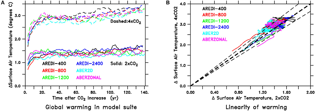
Figure 1. Time-series of temperature response under global warming run for all six A_REDI simulations. (A) Change in surface air temperature in °C. Solid lines denote simulations under 2xCO₂, dashed lines show the same simulations under 4xCO₂. (B) Change in surface air temperature under 2xCO₂ (horizontal axis) vs. change in surface air temperature under 4xCO₂. 2:1 Line is shown by thick dashed line. Points lying within thin dashed lines are within 10% of a 2:1 relation, meaning that the response under 4xCO₂ would predict the response under 2xCO₂ to within about 10%.

The relatively weak dependence of the warming on mixing is somewhat surprising, given that the initial climate states differ by up to 1.2°C. We computed the initial radiative forcing F associated with quadrupling CO₂ (ranging between 6.11 and 7.22 W/m²) by regressing changes in net radiation at the top of the atmosphere against global temperature change (following Gregory et al., 2004). This is consistent with the 6.72 W/m² value found by Andrews et al. (2012) for the higher-resolution ESM2M and sits within the 5.85–8.5 W/m² found across 11 CMIP5 models. However, the range in initial radiative forcing is balanced by a similar range in how strongly the climate warms in response to that forcing, so that the equilibrium climate sensitivities under doubling range between 1.9 and 2.1°C, on the low end of the CMIP5 range. We defer a more in-depth discussion of these results to a future manuscript. For now, it is sufficient to note that our model has a typical radiative response to increasing CO₂ and that our 4xCO₂ simulations lie in between the Representative Concentration Pathways (RCP) 6.0 and 8.5 in CMIP5, while our 2xCO₂ simulations lie between the RCP2.6 and RCP4.5 pathways.

Weak Dependence of Surface Chemistry on Mixing in Control Simulations Outside Northern Subpolar Latitudes

A relatively weak sensitivity of the model to the representation of A_REDI is also found when examining the distribution of surface chemistry averaged over the final century of each simulation. As shown in Figure 2, the models capture large-scale spatial patterns of zonally-averaged annual mean macronutrient, total alkalinity Alk, and calcite supersaturation compared to observations (observed zonally averaged annual iron is not shown because of data sparsity). The largest disagreements amongst the models, as well as between the models and observations, are found in subpolar latitudes between 40 and 60°N. This is largely driven by the North Pacific subpolar gyre, where iron limitation appears to be much weaker in the model than in the real world (Nishioka, 2007). Increasing mixing produces higher macronutrients, particularly in the northern subpolar latitude band (Figure 2A). The low-mixing simulation, AREDI-400 (black line) has the lowest values, and thus the biggest underestimate relative to observations while ABERZONAL (purple line) produces macronutrient surface estimates closest to observations.

FIGURE 2

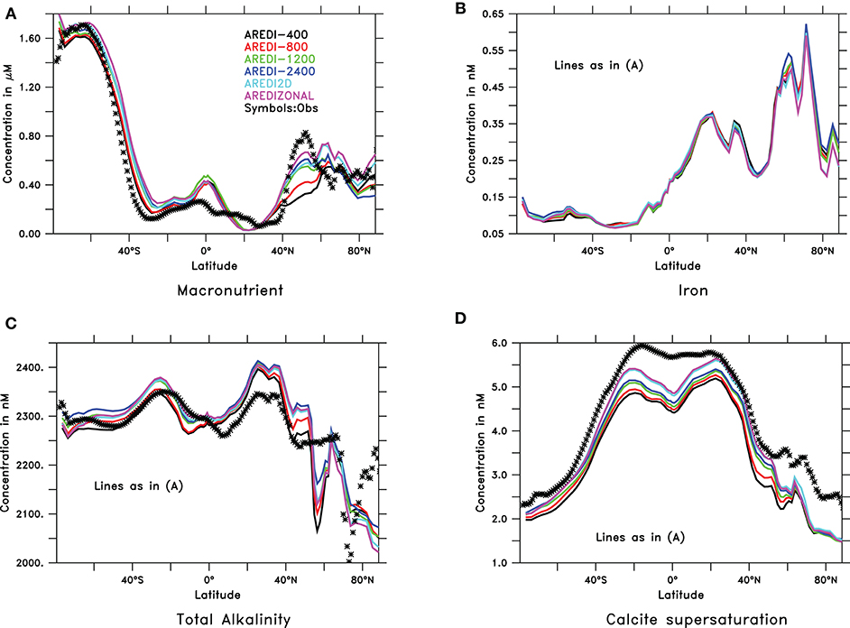
Figure 2. Zonally averaged annual mean surface chemical fields in CM2Mc pre-industrial control run with six different A_REDI parameterizations compared to observations (symbols). Iron observations are not included due to a lack of reliable data. (A) Phosphate [μM, obs. from WOA09, Garcia et al. (2010)] (B) Iron (nM), (C) total alkalinity [μM, obs from Lauvset et al. (2016)], and (D) calcite supersaturation [non-dimensional, obs from Lauvset et al. (2016)].

The other hydrographic variables show less sensitivity to mixing. Iron (Figure 2B) and alkalinity (Figure 2C) both show relatively small differences across models, though Alk appears to increase with greater mixing. All the models simulate the zonal range of calcite supersaturation in surface waters, as seen in Figure 2D, however, all models underestimate the degree of calcite supersaturation relative to modern observations.

Dependence of Surface Biological Cycling on Mixing in Control Simulations

Chlorophyll Shows Weak Dependence on Mixing Outside Northern Subtropical Region

We now turn to how our mixing parameterizations affect integrative measures of ecosystem function that can be characterized using remote sensing. Despite major uncertainties in retrieval algorithms, the fact that satellites can monitor such fields with high spatial and temporal resolution allows for detection of global and regional trends. In this paper we consider a number of these variables that have been used to characterize global change. We start with Chl because it is relatively easy to detect from space and has been extensively examined for trends (e.g., Gregg et al., 2005; Henson et al., 2010; Rykaczewski and Dunne, 2011).

As is the case for nutrients, the modeled concentration of Chl in our suite (Figure 3A) is only moderately sensitive to the parameterization of A_REDI. All models capture the observed contrast between upwelling and downwelling regions and show broad similarities to observations in the Southern Ocean and the tropics. The models all overestimate Chl in the northern subtropics from 30 to 45°N. The largest sensitivity to mixing is found in these latitudes as well, with increasing mixing producing chlorophyll levels up to 50% higher than those seen in AREDI-400.

FIGURE 3

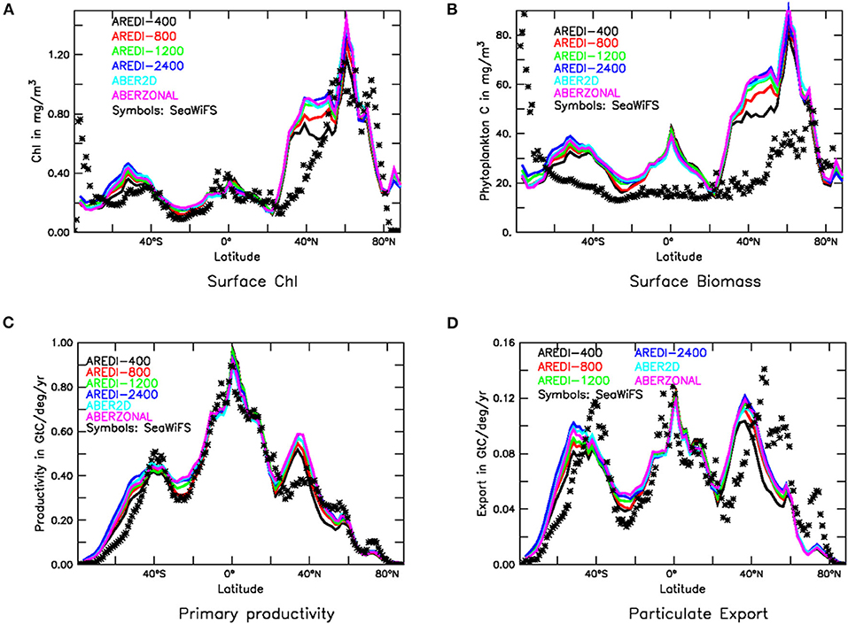
Figure 3. Biological fields in CM2Mc pre-industrial control run with six different A_REDI parameterizations (colored lines) compared with satellite-based estimates (symbols). (A) Zonally averaged chlorophyll (mg/m³). (B) Zonally averaged particulate carbon (mg/m³). (C) Zonally integrated primary production (GtC/yr/deg) and (D) Zonally integrated particle export across 100 m (GtC/yr/deg). Satellite estimates in (A,C,D) are taken from Dunne et al. (2007). Particulate carbon in (B) is estimated from backscatter following Behrenfeld et al. (2005).

Biomass Shows Weak Dependence on Mixing Outside Northern Subtropical Region

Chl suffers from one major problem as a measure of ecosystem function. Because phytoplankton can change their chl:C ratio to match the availability of nutrients (Geider et al., 1996), a decline in Chl in response to an increase in light availability may not represent a decline in the total amount of biomass in an ecosystem. For this reason, we also examine the total phytoplankton biomass, which can be estimated from particulate backscatter (symbols Figure 3B). Biomass serves as an index commonly used by fishery experts to monitor ecosystem response to climate change (e.g., Cabré et al., 2015a) and regional trophic interactions (Kwiatkowski et al., 2018). Note that the “observed” biomass in Figure 3B does not show a peak in the equatorial zone, which may be due to problems with the retrieval algorithm used to estimate the backscatter [alternative estimates of biovolume such as Kostadinov et al. (2009), show a clear signature of equatorial upwelling].

As seen by the colored lines in Figure 3B, zonally averaged phytoplankton biomass is also relatively insensitive to mixing parameterization, except in the northern subtropics from 30 to 45°N. Within this latitude band, macronutrients are not typically overestimated (Figure 2A), so it is possible that both the high Chl and biomass concentrations indicate overly high iron concentrations. As with chlorophyll, increasing mixing produces increasing biomass, with the highest mixing models predicting surface biomass in the northern subtropics that is ~40% higher than in AREDI-400.

Primary Productivity and Particle Export Show Weak Sensitivity to Mixing

Tracing the flow of carbon and nutrients through an ecosystem is generally done using measures of productivity. One such measure is the primary productivity, representing the uptake of carbon by phytoplankton (Chavez et al., 2011), for which many satellite-based estimates exist in the literature (Saba et al., 2011). However, a more appropriate index for detecting bottom-up ecological change on longer timescales may be the particle export (Laufkötter, 2016; Buesseler et al., 2020). This is because export to the deep ocean is more sensitive to grazing from large zooplankton that transfer energy up the food web to fish and also drive the chemistry and biology of the deep ocean (Jones et al., 2014).

Primary productivity and particle export [which are compared with satellite-based estimates from Dunne et al. (2007) in Figures 3C,D] are much less sensitive to mixing than chlorophyll and biomass. They are also relatively close to observations. The models all show similar levels of productivity and export as the (relatively uncertain) observations, with peaks in at around 40°S, on the equator and at 40°N. Primary productivity is well-simulated in all the models, with the exception of models overestimating it in the northern subtropics from 30 to 45°N, the same region where chlorophyll and biomass appear to be too high in Figures 3A,B. Zonally integrated particle export flux observations peak at 0.12 Gt C/yr/deg of carbon per year in the Southern Hemisphere (SH) and 0.14 Gt C/yr/deg in the NH. The models show peaks that are slightly smaller and shifted southward in both hemispheres. As noted in Bahl et al. (2019), globally integrated values of export production in the model suite (which range from 9.95 GtC yr⁻¹ in AREDI-400 to 11.1 GtC yr⁻¹ in AREDI-2400) lie well within the range of satellite estimates: of 9.8 GtC yr⁻¹ ± 20% estimated by Dunne et al. (2007).

Globally Integrated Biological Responses to Increased CO₂

Different Globally Integrated Indices of Biological Cycling Show Differing Sensitivities to Warming and Mixing

On a global scale all four of the indices of surface biological cycling described in Figure 3 decrease under global warming. An examination of relative changes in these indices (Figure 4) shows that the bulk of the adjustment to the new equilibrium occurs over the first 40–60 years. Further examination of Figure 4 reveals several important results.

FIGURE 4

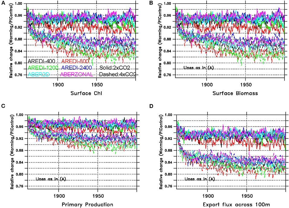
Figure 4. Time series of relative changes in biological variables under doubled and quadrupled CO₂ for the different A_REDI parameterizations shown as a ratio of high CO₂/control. Upper group of lines are for doubled CO₂, while lower group shows changes under quadrupled CO₂. (A) Global surface chlorophyll change. (B) Global surface biomass change. (C) Global primary productivity change. (D) Global export across 100 m.

First, although the sign of the decrease is the same across all variables, the magnitude of the decrease is quite different, with primary production (Figure 4C) showing much smaller changes than chlorophyll, biomass and export production (Figures 4A,B,D). This suggests that some fraction of the declines in biomass are partially compensated by higher temperatures resulting in faster metabolic rates [larger exp(k*T)]. It also points out that using primary productivity as an index of climate change [as in Chavez et al. (2011)] may underestimate potential ecosystem impacts.

Second, there is a greater spread across models for the relative changes in the biological variables than there was for global mean temperatures in Figure 1, with much less distinction between the 4xCO₂ and 2xCO₂ simulations. Uncertainty about mixing contributes most strongly to uncertainties in surface chlorophyll and primary productivity, where the inter-model range (6 and 4%, respectively) is comparable to the drop due to doubling CO₂. Conversely, uncertainty about mixing contributes less strongly to surface biomass and global export change where a much clearer separation between the 2xCO₂ and 4xCO₂ cases is seen.

Third, the within-scenario spread across models is consistent across the different variables. Models with a larger relative decrease in chlorophyll have larger decreases in all the other variables as well.

Finally, the size of the changes does not appear to be monotonic with increasing mixing, with the AREDI-800 case showing the largest drop under doubling and AREDI-800 and AREDI-1200 cases showing the largest drops under quadrupling. In general, the ABER2D and ABERZONAL simulations behave more like the high-mixing models than the low-mixing models.

Response of Global Indices Is Relatively Linear, Some Are Moderately Sensitive to Mixing

Because it is difficult to extract patterns from these time series plots, we summarize the results by averaging over years 40–140 and presenting the results as bar plots in Figure 5. In each subplot, fractional changes under 2xCO₂ are shown on the left, and ½ of the change under 4xCO₂ is shown on the right. When bars of different colors within a particular region and scenario are of different lengths, this indicates that A_REDI (model uncertainty) plays an important role in explaining intermodel variability. If corresponding collections of bars in different scenarios have different lengths this indicates that the linearity assumption used to hindcast historical changes from 4xCO₂ changes is violated. If collection of bars is a perfect rectangle then there is no sensitivity to mixing, whereas if the bars within a cluster have vastly different lengths the sensitivity to mixing is strong. In addition to the four indices used in Figure 4, we also look at the changes in the biomass of large phytoplankton which are disproportionately important for feeding energy to higher trophic levels. Some models have suggested that trophic interactions can amplify changes in large phytoplankton biomass to produce relatively larger changes in total biomass (Lotze et al., 2019).

FIGURE 5

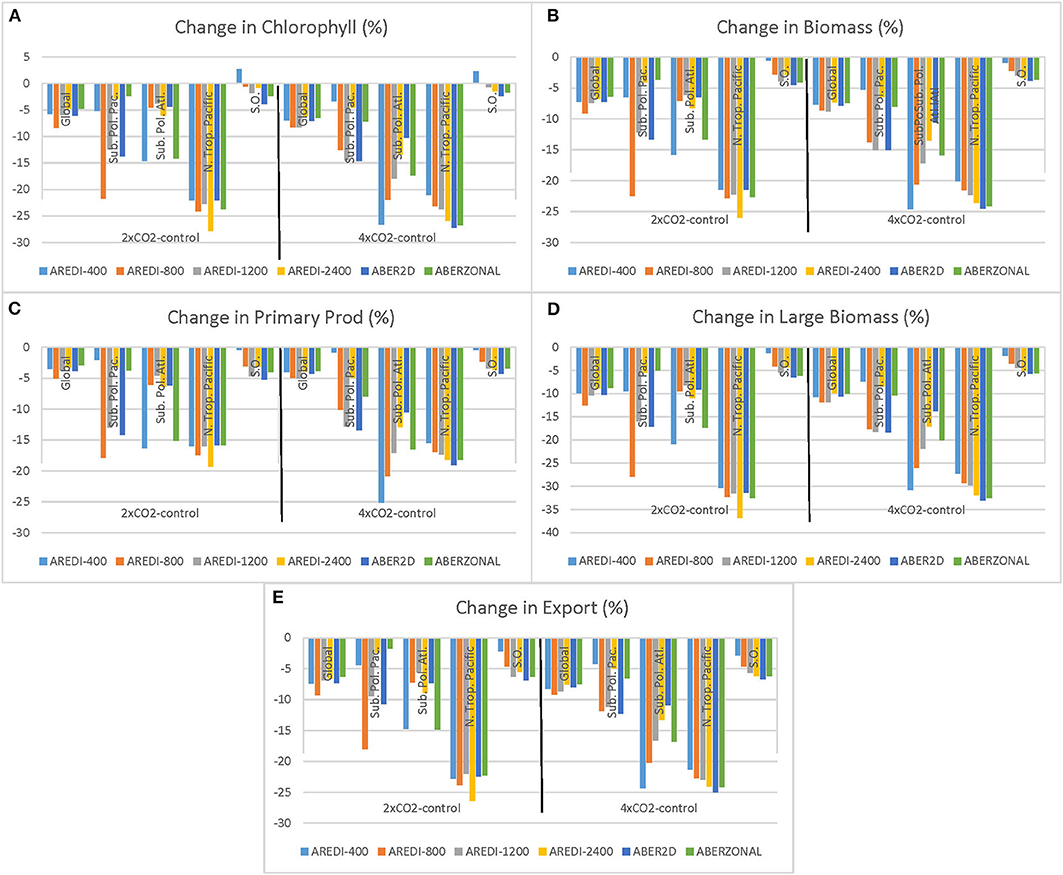
Figure 5. Summary of changes in biological variables across models and scenarios. Each plot shows the relative change in % for (A) Chlorophyll, (B) Biomass, (C) Primary Production, (D) Large Biomass, and (E) Export. Each plot is divided into results from 2xCO₂ simulations (left half) and ½ the change under the 4xCO₂ simulation (right half). Each cluster of bars shows changes in a particular region across models (colors denote different distributions of A_REDI). Clusters from left to right within each half plot show the global integral, the Subpolar North Pacific from 40 to 60°N, the Subpolar North Atlantic from 40 to 60°N, the Northern Tropical Pacific (10-25°N, site of the largest drops in biological variables in Figure 8), and the Southern Ocean (70-50°S).

As in Figure 4, the magnitude of the decline in biological activity under global warming (Figure 5, bars marked “Glob” in each subplot) depends on the index. Primary productivity is the least sensitive of any of the global indices to warming, with declines on the order of 4% under doubling and 8% under quadrupling (Figures 4C, 5C). The biggest changes are seen in large phytoplankton biomass (Figure 5D), which drops 8–12% in the 2xCO₂ case and 20–24% in the 4xCO₂ case. Chl (4–8% drop under doubling, 12–16% under quadrupling), total biomass (~8% under doubling, ~16% under quadrupling), and particle export (~8% under doubling ~18% under quadrupling) lie in between these extremes.

In general, the responses of the global indices to increasing radiative forcing is relatively linear. There is some hint of non-linear responses in the global Chl field, with the cluster of bars marked “Glob” on the left-hand side of Figure 5A noticeably smaller than those on the right-hand side. This is not the case, however, for the other indices, indicating that the response at 2xCO₂ is roughly half the response at 4xCO₂.

There is some sensitivity, however, to the mixing parameterization as each cluster of bars shows intra-cluster variability. As would be expected from Figure 4, this is biggest for surface chlorophyll, where the 4% intermodel range under 2xCO₂ is 2/3 of the ~6% drop. However, for the other variables, the relative range across the models is smaller. There is also some sense that the relative range across models is smaller for the 4xCO₂ cases than the 2xCO₂ cases (each cluster of bars marked “Glob” is more squared off on the right-hand side of each subplot). It is worth noting that the models do not show a monotonic dependence on mixing, with bar lengths sloping down to the left or to the right within each cluster. Instead, all clusters show the strongest sensitivity for AREDI-800 (orange bars) and the weakest for ABERZONAL (green bars).

Regional Response to Increased CO₂ Across Models

Although the global responses are relatively linear and at most moderately sensitive to mixing, this is not always true for regional changes. For instance, relative changes in the zonally averaged biological variables (Figure 6, compare with Figure 3), reach magnitudes of up to 50% with a strong dependence on mixing. We examine these regional changes in more detail below.

FIGURE 6

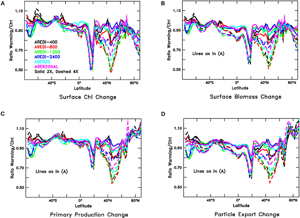
Figure 6. Relative changes in zonally averaged biological fields under global warming (paralleling Figure 3), averaged over years 40–140 of high CO₂ simulations. Solid lines show 2xCO₂, dashed lines 4xCO₂. (A) Chlorophyll, (B) Particulate carbon, (C) Primary productivity, and (D) Particle export across 100 m.

Different Regions Respond Differently to Mixing and Increased CO₂

One latitude band that stands out in Figure 6 is between ~40 and 65°N in NH subpolar latitudes. This region exhibits large reductions in Chl, particulate carbon, primary productivity, and particle export that also depend on the mixing parameterization. Under 4xCO₂, the largest drops are seen in AREDI-400 and AREDI-800, with AREDI-2400 showing the smallest drops and ABER2D and ABERZONAL lying in between. Returning to Figure 5, we see that the changes in the zonal mean do not reflect zonal uniformity, as there are large differences between the subpolar North Atlantic (bars marked “SubPolAtl”) and the subpolar North Pacific (bars marked “SubPolPac”) for all of the variables. Each basin shows quite different sensitivities to mixing, with the largest changes in the 2xCO₂ simulations in the subpolar North Pacific occurring in the AREDI-800 simulation, but in the AREDI-400 and ABERZONAL simulations in the subpolar North Atlantic.

Northern subpolar indices of biological cycling respond non-linearly to increased CO_2. Changes in the subpolar North Atlantic in the 2xCO₂ simulations would be greatly overestimated by extrapolating from the 4xCO₂ simulations for AREDI-800, AREDI-1200, AREDI-2400, and ABER2D, as would changes in the subpolar North Pacific for AREDI-1200. On the other hand, changes in the subpolar North Pacific in AREDI-800 (orange bars, Figure 5) in the 2xCO₂ case would be underestimated by extrapolating from changes in the 4xCO₂ case.

A second large drop in Chl, biomass, and productivity is found at about 15°N, but in contrast to the changes in the northern subpolar latitudes, the changes in this region are relatively insensitive to the mixing parameterization as the different lines overlay each other. Moreover, although the changes shown in Figure 6 are larger under 4xCO₂ than under 2xCO₂, examination of the bars marked N. Trop. Pacific in Figure 5 shows that the responses across models are relatively linear and that the changes in the 2xCO₂ simulations can be relatively well-predicted from changes in the 4xCO₂ simulations.

In the Southern Ocean, mixing has a big impact on the biological response. The AREDI-400 simulation shows a small increase in Chl and small decreases in total biomass, primary productivity, and export. As the mixing increases, we see a loss of Chl under increased CO₂ and larger decreases in biomass, primary productivity, and export. However, the responses appear to be relatively linear across the 2xCO₂ and 4xCO₂ cases (bars marked SOcean in Figure 5).

Different Responses of Nutrients to Climate Change by Latitude

In this subsection we examine how climate change produces changes in nutrients. Increasing CO₂ reduces macronutrient (Figure 7A) across nearly all latitudes with the 4xCO₂ scenarios producing larger decreases than the 2xCO₂ scenarios. Cabré et al. (2015a) show similar declines in nitrate in most biomes across CMIP5 models. The biggest decreases in our suite are seen in the subpolar NH. However, macronutrients rise in the Southern Ocean, most likely due to increased upwelling associated with stronger winds under global warming.

FIGURE 7

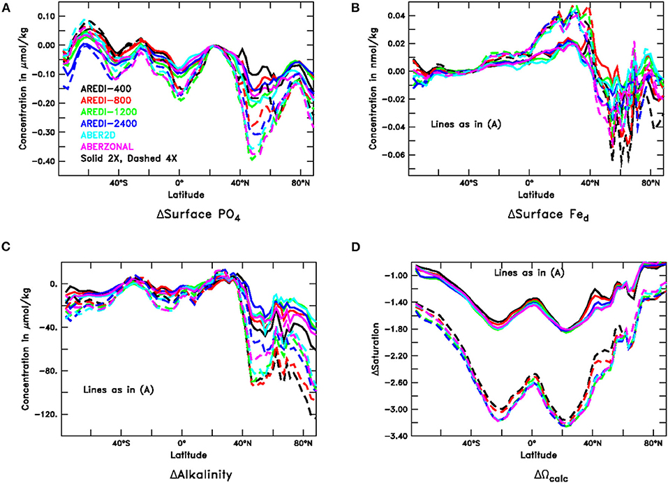
Figure 7. Changes in surface chemical properties for years 40–140 of high CO₂ simulations. Solid lines represent changes under doubled CO₂; dashed lines represent changes under quadrupled CO_2. (A) Phosphate (μM). (B) Dissolved iron (nM). (C) Alkalinity (μM). (D) Calcite supersaturation (non-dimensional).

Dissolved iron (Figure 7B) shows a very different picture with little variation across models outside the northern subpolar latitudes. Somewhat surprisingly, increasing CO₂ increases iron in the sub-tropics, presumably because with lower nutrients (and export) there is less biological removal. The spatial distribution under 4xCO₂ is well-correlated with changes under 2xCO₂. In the subpolar northern hemisphere, iron decreases across scenarios but is strongly modulated by mixing, with an overlap between the 2xCO₂ and 4xCO₂ cases.

Regional Patterns of Biomass Change in the AREDI-400 and AREDI-2400 Models Involve Changes in Both Light and Nutrient Limitation

As is already clear from looking at basin-averaged changes in the subpolar NH, zonally averaged differences shown in Figures 6, 7 are a crude representation of a more complex pattern of changes. These patterns are broadly similar in sign across simulations but have different magnitudes in different regions. This can be seen by looking at Figure 8, which shows relative changes in biomass between the 4xCO₂ simulation and control simulation for the low-mixing AREDI-400 case (top row) and high-mixing AREDI-2400 case (bottom row). Looking at changes in total phytoplankton biomass in Figures 8A,C, we see that both simulations project small (<20%) increases in total phytoplankton biomass in the Arctic, Southeast Atlantic Ocean offshore of the Benguela upwelling, the Gulf of Mexico, parts of the Southern Ocean along the coast of East Antarctica, and the Sea of Okhotsk. However, these increases are offset by large decreases in the North Atlantic and Pacific, with a particularly intense band of decrease just south of 20°N (corresponding to where Chl, biomass, and productivity decrease in Figure 6). The magnitude of changes is generally larger in AREDI-400 than in AREDI-2400. A few regions (for example the Ross Sea) see opposite-sign changes in biomass.

FIGURE 8

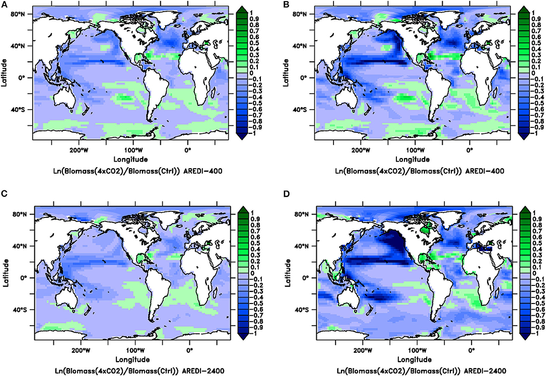
Figure 8. Relative changes (natural log of the quotient of the value in century-long climatology of the 4xCO₂ run over the value in a century-long climatology of the Control) in total phytoplankton biomass (left column) and large phytoplankton biomass (right column) for the AREDI-400 case (top row) and AREDI-2400 case (bottom row). (A) Relative change in total phytoplankton biomass for the AREDI-400 case, (B) Relative change in large phytoplankton biomass for the AREDI-400 case, (C) relative change in total phytoplankton biomass for the AREDI-2400 case, and (D) relative change in large phytoplankton biomass for the AREDI-2400 case. Small values are effectively fractional changes. The color bar denotes the size of the logarithmic change, so that blue denotes lower biomass; green denotes higher biomass.

The impact of quadrupling CO₂ is much greater when we focus on large phytoplankton biomass (Figures 8B,D). Both the low- and high-mixing models show steep reductions in large phytoplankton biomass throughout the North. Equatorial current, moving into the Kuroshio current and south into the East Australia Current. The effects can also be seen in the North Atlantic current. However, the low-mixing model appears to project larger reductions in the North Atlantic and the North Pacific, whereas the AREDI-2400 model (Figure 8D) projects regional decreases that are smaller due to greater persistence of deep convection. The changes, however, are not found in the center of the convective regions [which Pradal and Gnanadesikan (2014) and Bahl et al. (2019) showed are found in the Northwest Pacific] or the equatorial upwelling zones. Instead, the big drops in biomass in the North Pacific are found at the edges of these high nutrient regions. This is consistent with Oschlies (2002), who found the gyre edges experience large relative changes in nutrients.

To better understand these changes, we revisit Equation (5), which shows that the biomass in BLING is regulated by the product of a nutrient limitation term and a light limitation term. The spatial distribution of the changes in these limitation terms under quadrupled CO₂ is shown for AREDI-400 and AREDI-2400 cases in Figure 9. Both models show broadly opposite patterns of change for light and nutrient limitation, such that regions with more light limitation have less nutrient limitation and vice-versa. Different biological limitations dominate in different regions. In the Arctic, reduction of light limitation causes biomass and productivity to increase in both models. By contrast, greater nutrient limitation is likely responsible for the decreases in phytoplankton biomass in the North Pacific and subpolar North Atlantic seen in Figures 5, 8.

FIGURE 9

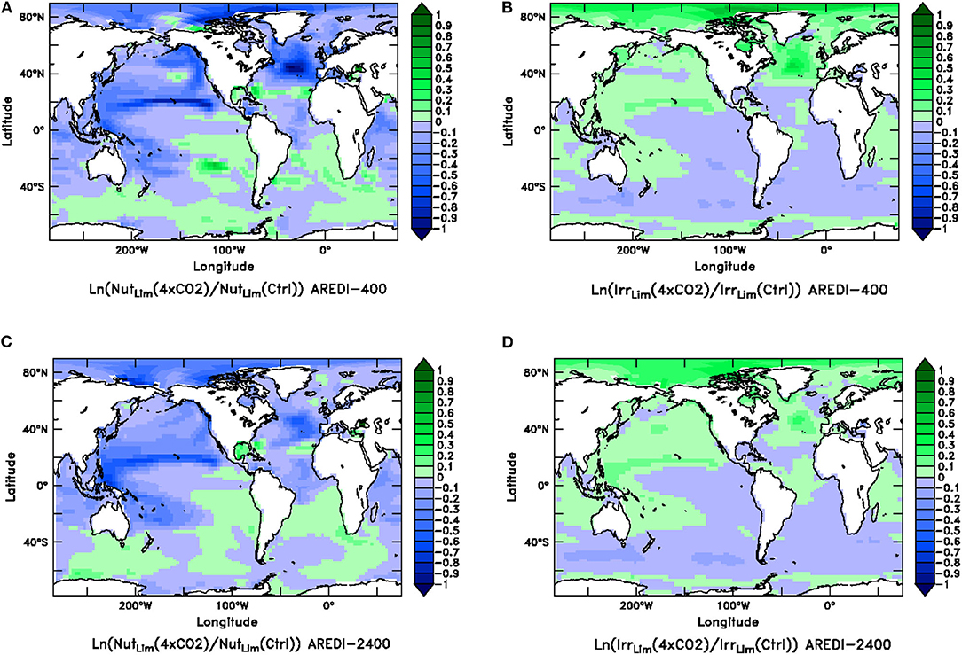
Figure 9. Relative changes (natural log of the quotient of the value in century-long climatology of the 4xCO₂ run over the value in a century-long climatology of the Control) in the ratio of the quadrupled CO₂ case and the control for the nutrient limitation term (left column) and the light limitation term (right column) for the AREDI-400 case (top row) and AREDI-2400 case (bottom row). (A) Nutrient limitation for the AREDI-400 case, (B) light limitation term for the AREDI-400 case, (C) nutrient limitation for the AREDI-2400 case, and (D) light limitation term for the AREDI-2400 case. As the growth rate is the product of these terms, low values mean higher limitation, so that blue denotes lower nutrients or lower light while green denotes higher nutrients or higher light.

What gives rise to these different spatial patterns of limitation? In the North Tropical Pacific, greater nutrient limitation is primarily caused by a ~50% drop in macronutrient concentrations in the equatorial upwelling. Because macronutrients are relatively high along the equator this produces only a small change in nutrient limitation there, but once the nutrients are moved away from the equator they run out much more quickly in the 4xCO₂ simulation. The peak of easterly wind stress to the north of the equator also drops by about 10% in the 4xCO₂ case, resulting in less advection of nutrient-rich water northward and less upwelling of nutrient-rich water from below. These changes are relatively similar across the simulations with different A_REDI.

In the subpolar North Pacific, macronutrient is brought up on the northwestern corner of the basin, but is redistributed by the subpolar gyre, with the lowest concentrations in the east. In the AREDI-400 case, quadrupling CO₂ reduces the concentration to the west of the dateline in the latitude band from 40 to 60°N from 0.4 to 0.3 μM (well above the half-saturation coefficient of 0.1 μM). However, to the east of 150°W in the same latitude band quadrupling CO₂ produces a smaller absolute change (from 0.034 to 0.014 μM) but a significant relative change both in nutrient and in the corresponding limitation term. As a result, the relative decline in biomass is much larger here.

By contrast, stronger light limitation (which is driven by more cloudiness–not shown) is responsible for the declines in biomass seen within the Southern Ocean. The somewhat surprising result that nutrient limitation decreases in the Southern Ocean in AREDI-400 is partly attributable to these decreases in light, but also to enhanced winds leading to more upwelling bringing more iron to the surface at around 60°S (see also Figure 7B). By contrast in AREDI-2400, decreases in vertical mixing result in a reduced supply of nutrients.

Mixing Is Important for Understanding Indices of Interior Habitability in Both the Control and Global Warming Simulations

Although uncertainty in mixing has a relatively small impact on global-scale biological indicators in the surface layers, we know from previous work that this is not necessarily true for the ocean interior. Gnanadesikan et al. (2013) and Bahl et al. (2019) demonstrated that mixing has a big impact on the magnitude and climate sensitivity of oceanic hypoxia (defined here as oxygen concentration >2 ml/l or 88 μM). In this section we extend this work to look at carbonate undersaturation, which like hypoxia, occurs where the products of respired sinking organic material are allowed to accumulate (Gobler and Baumann, 2016). However, in contrast to hypoxia, the calcite saturation state is a function of pressure (Zeebe and Wolf-Gladrow, 2001), and thus will be more strongly affected by small increases in remineralized nutrients and carbon at depth. We also examine the linearity of the response of both parameters, evaluating whether historical changes can be predicted by large-amplitude increases in atmospheric carbon dioxide. Given that the pre-industrial control models show relatively weak sensitivity to mixing in their surface carbonate saturation state (Figure 2D), surface concentrations of alkalinity (Figure 2C), and particulate export (Figure 3D), we might expect that interior differences in hypoxia and calcite undersaturation would also be small across models.

In fact the range of depths experiencing either calcite undersaturation or hypoxia is strongly affected by the value of A_REDI. This is particularly clear in the North Pacific where observations (Figures 10A,B) show hypoxic waters occupying as much as 2,000 m of the water column, while calcite-undersaturated waters occupy more than 4,000 m in some locations. High levels of calcite undersaturation are expected in the North Pacific where the oldest deep waters with the largest accumulation of acidic remineralized carbon are found. The ability of the models to simulate these environments is not very good and is sensitive to different rates of ventilation. In the AREDI-400 model hypoxic depth ranges up to 4,500 m are found, but the highest values are found in the Eastern Pacific, as well as a second intense center in the Bay of Bengal. By contrast, the high-mixing case (AREDI-2400) simulates a significantly smaller hypoxic volume with a depth range that does not exceed 2,000 m, shown in Figure 10E. This is a somewhat of a common bias amongst models (Gnanadesikan et al., 2013; Cabré et al., 2015b; Bahl et al., 2019). The global volume of calcite-undersaturated waters (Figures 10D,F) is somewhat better simulated in AREDI-400, though the volumes in the subpolar North Pacific are too small and those in the equatorial Pacific too large. The AREDI-2400 model also simulates a significantly smaller volume of calcite-undersaturated water in both regions.

FIGURE 10

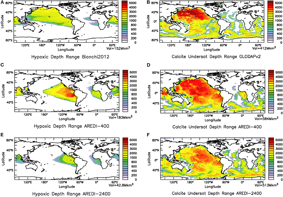
Figure 10. Influence of mixing coefficient on mean-state hypoxia and calcite undersaturation. (A) Observations, taken from Bianchi et al. (2012), of depth of water in m column occupied by hypoxic waters and (B) observations from GLODAP (Lauvset et al., 2016) of the depth of the water column in m over which calcite undersaturation is found. (C) Hypoxic depth range for low-mixing model AREDI-400, (D) depth range of calcite undersaturation for low-mixing model AREDI-400, (E) Hypoxic depth range for high-mixing model AREDI-2400, and (F) depth range of calcite undersaturation for high-mixing model AREDI-2400.

Changes in the global volume of hypoxic and calcite-undersaturated waters are very sensitive to the parameterization of mixing, and deviate from perfect linearity. As shown in Figure 11A, hypoxic volume expands the most for the AREDI-400 model under 2xCO₂ and actually contracts in the AREDI-1200 models [also reported in Bahl et al. (2019)]. A novel result in this paper is our finding that changes in hypoxic volume cannot simply be scaled down from the 4xCO₂ cases. Doing so underestimates the change in hypoxic volume in the 2xCO₂ case for all the cases other than AREDI-1200 (gray bars in Figure 11A are smaller than the blue bars). For AREDI-1200, hypoxia expands slightly in the 4xCO₂ case but shrinks in the 2xCO₂ case. The fact that it is difficult for ESMs to consistently reproduce the observed trends of hypoxic water expansion, particularly in the tropical OMZs (Bahl et al., 2019), may in part stem from this underlying non-linearity [though as noted by Andrews et al. (2017), other mechanisms such time-varying stoichiometry may also play a role].

FIGURE 11

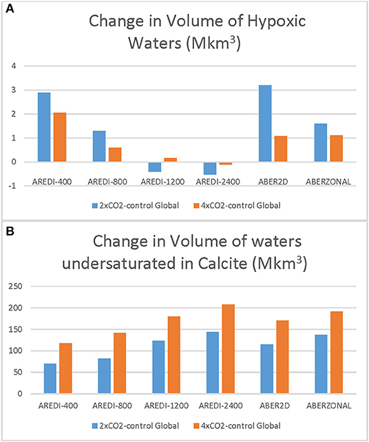
Figure 11. Absolute changes in the volume of hypoxic waters (A) and waters undersaturated with respect to calcite (B) in Mkm³. Blue bars show response under 2xCO₂. Gray bars show half of the response under 4xCO₂-differences from blue bars show lack of linearity.

The global volume of calcite-undersaturated water shows a different pattern of change in Figure 11B, with undersaturated waters increasing for all of the values of A_REDI in both the 2xCO₂ and 4xCO₂ simulations. The biggest increases in global calcite undersaturation are seen for AREDI-2400, which predicts 929 Mkm³ of undersaturated water in the 4xCO₂ case, an 80% increase from 513 Mkm³ volume in the pre-industrial control simulation. By contrast, the AREDI-400 case shows an undersaturated water volume of 654.2 Mkm³ under doubling and 816 Mkm³ under quadrupling vs. 584 Mkm³ in the pre-industrial control. Note that in contrast to the hypoxic volume, the 4xCO₂ calcite undersaturation change overpredicts the 2xCO₂ change for all values of mixing.

The spatial pattern of changes in calcite undersaturation are shown in Figure 12 for the AREDI-400 and AREDI-2400 models. Both models show an increase in the volume of undersaturated water in the North Pacific, qualitatively consistent with recent observational trends (Feely et al., 2004). In AREDI-2400 the impact of a collapse in deep convection is clearly seen, with depths of calcite undersaturation expanding by over 2,000 m. The AREDI-400 model has much smaller changes in the Pacific, but actually shows larger changes in the Southeast Atlantic. Due to a lack of accumulation of respired CO₂ the North Atlantic remains supersaturated in all four runs. In the Indian Ocean, the depths of calcite undersaturation expand as both CO₂ and mixing increase. These differences suggest that calcite undersaturation is one field for which uncertainty in A_REDI may contribute strongly to uncertainties in future projection–with important implications for deep-sea organisms (Bach, 2015).

FIGURE 12

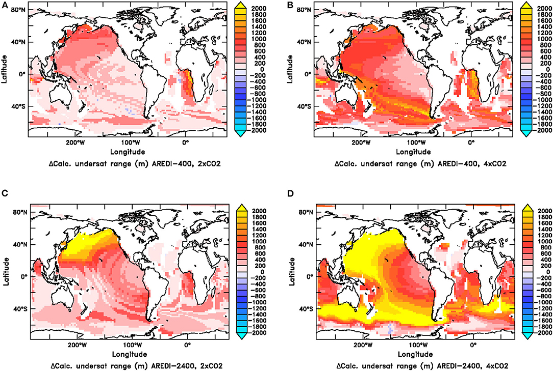
Figure 12. Change in the vertical extent of the water column over which calcite undersaturation is found for the 2xCO₂ (A,C) and 4xCO₂ (B,D) simulations for the AREDI-400 simulations (top row) and AREDI-2400 simulations (bottom row).

Convection Explains Why Subpolar Gyres and Interior Habitability Behave Non-linearly and Are Sensitive to Mixing

We have seen that in our model suite global measures of surface ecosystem function, in particular chlorophyll, are at most moderately sensitive to changes in mixing and vary relatively linearly with radiative forcing. However, interior measures of habitability such as hypoxia and calcite undersaturation are much more sensitive to mixing and vary non-linearly, just as subpolar changes in ecosystem cycling do. Moreover, we see that the volume of calcite-undersaturated water increases under global warming for all of our models, despite a decrease in export.

We can reconcile these apparently contradictory results by noting that the degree to which interior waters are low in oxygen and carbonate ion is not solely determined by the rate which oxygen and carbonate ion are consumed as a result of remineralization. It is also controlled by the amount of time over which remineralization is allowed to accumulate–the age of the water. The age is inversely related to the rate of vertical exchange in high latitude regions and thus is tightly linked to the magnitude of convection in the subpolar gyres. As discussed in Bahl et al. (2019), the increase in age under global warming explains the changes in interior oxygen under 2xCO₂ cases–overwhelming the impact of declining export. Figure 11B tells us this must be true for calcite undersaturation as well.

One way of characterizing the changes in age is by looking at Δ¹⁴C, which is insensitive to biological cycling. Low gradients in Δ¹⁴C between the surface and 1,500 m imply relatively rapid vertical exchange. As illustrated in Figure 13A, the North Pacific in the pre-industrial control simulation looks very different across our model suite. The AREDI-400 model has a vertical gradient over the top 1,000 m that is relatively close to the observed estimate from Key et al. (2004). The higher mixing models (AREDI-1200, AREDI-2400, ABER2D, and ABERZONAL) all simulate very low gradients of radiocarbon, implying unrealistically rapid vertical exchange. The AREDI-800 model (red line, Figure 13A) lies in between these two extremes.

FIGURE 13

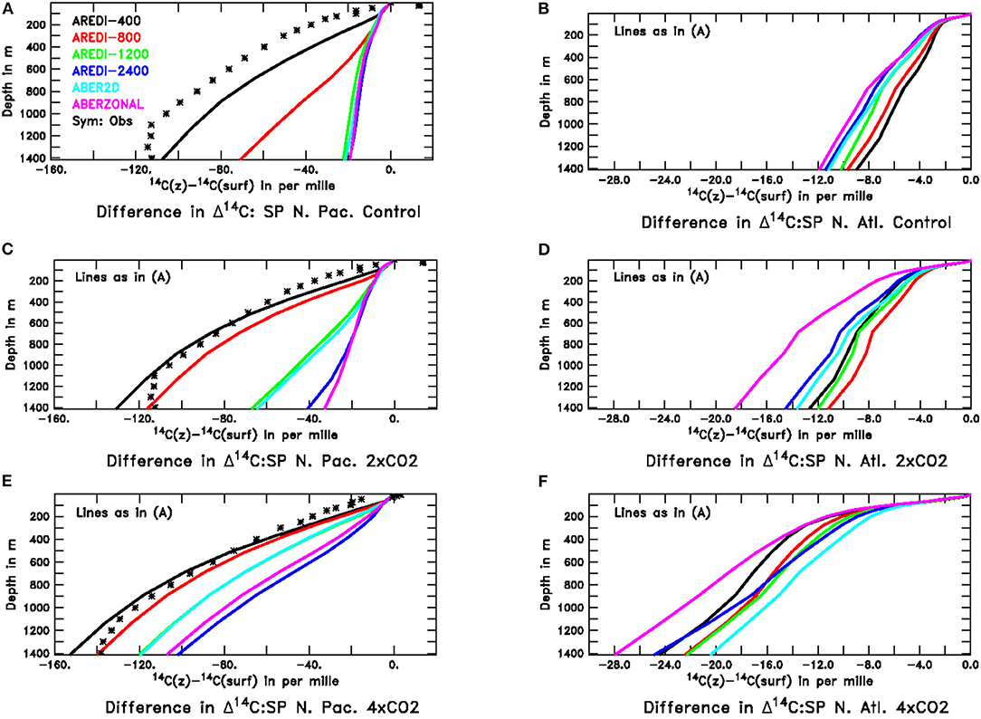
Figure 13. Profiles of radiocarbon relative to its surface value in the subpolar North Pacific and North Atlantic across our model suite. Observational estimates of pre-bomb radiocarbon from Key et al. (2004) are shown for the North Pacific with the symbols. For the North Atlantic the methods used to remove the signal of atmospheric nuclear testing do not work as well, and the deep ocean ends up having a higher radiocarbon concentration than the surface-a physically nonsensical result. For this reason we do not show the Key et al. (2004) estimates for this region. Top row shows the pre-industrial control simulations, middle row the 2xCO₂ simulations and bottom row the 4xCO₂ simulations. All model results are from century-long averages. (A) North Pacific, Control (B) North Atlantic, Control (C) North Pacific, 2xCO₂ (D) North Atlantic, 2xCO₂. (E) North Pacific, 4xCO₂ (F) North Atlantic, 4xCO₂.

Global warming causes increases in the vertical gradient of Δ¹⁴C but does not do so identically across models. In the 2xCO₂ simulations (Figure 13C), the vertical gradient increases most sharply for the AREDI-800 simulation, which as previously illustrated in Figure 5 shows the largest relative decline in chlorophyll, biomass, productivity, and export under this scenario. AREDI-1200 and ABER2D show a smaller increase in vertical radiocarbon gradient in the North Pacific in Figure 13 and a smaller decrease in surface biological cycling in Figure 5 (gray and blue bars). Under 4xCO₂, the biggest changes in the North Pacific radiocarbon gradient are seen in AREDI-1200 and ABER2D, which then also show the biggest relative drops in biological cycling in Figure 5. In the North Atlantic, by contrast, the largest changes in vertical radiocarbon gradient between the pre-industrial control and the 2xCO₂ case occur in the ABERZONAL and AREDI-400 cases, while AREDI-800 is relatively unchanged. It is thus unsurprising that it is the AREDI-400 and ABERZONAL cases that show the largest relative drops in biological cycling within subpolar North Atlantic (Figure 5).

The reasons for the changes in convection are complex and regionally dependent. As discussed in Bahl et al. (2019), an increased hydrological cycle under global warming acts to decrease the density of high latitude surface waters reducing convection. On the other hand, reduction in sea ice (which occurs across all the models for both hemispheres under both scenarios), exposes more open water in the wintertime, leading to more heat loss and increasing the potential for convection. Finally, because the overturning in the North Hemisphere involves a transformation of light to dense water which must balance the transformation of dense to light water in the Southern Hemisphere, the decline in the overturning in the North Pacific can be counterbalanced by the increase in the North Atlantic. A full discussion of these processes is beyond the scope of this paper.

Discussion

A key part of applying ESMs to ecology (a primary goal of this special issue) is understanding where, when and why model responses will be non-linear. This work has focused on the extent to which uncertainty in the parameterization of lateral mixing, which has major impacts on the distribution and sensitivity of deep convection, can propagate into uncertainty in simulating ecosystem functioning and habitat distribution.

Before discussing the impact of mixing in more detail, we show that our estimates of changes in biological cycling are broadly consistent with those seen in the literature, although the decreases under global warming may be significantly larger or smaller than those seen in individual models. On the one hand, our 12–16% drops in Chl under 4xCO₂ are much smaller than the projected 50% decline in Chl associated with a 6°C increase in temperatures by Hofmann et al. (2011) in an intermediate complexity ESM. This is true even when the Chl change in Hofmann et al. (2011) is scaled down by a factor of two to match our changes in temperatures. On the other hand, the ~16% drops in surface biomass under 4xCO₂ are more extreme than the ~8% drop in biomass seen in two climate models for the RCP8.5 scenario by Lotze et al. (2019). Also using the RCP8.5 scenario, Bopp et al. (2013) reported declines in global primary production ranging from 0.9 to 16.1% (with mean of 8.6%) and Heneghan et al. (2019) presents a global decline of 5%. Our changes of 4% under doubling and 8% under quadrupling lie well within this range. Similarly, our changes in particle export of 5–6%/degree lie within the 3–15%/degree warming reported in Cabré et al. (2015a).

The fact that our estimates for the decline in global Chl, biomass, primary production and export cluster around a relatively small range compared to other estimates in the literature suggests that the range of responses in CMIP5 models is due to something other than lateral mixing. Although neglected in our model, one possible driver is the differential metabolic responses of phytoplankton and zooplankton to temperature. Taucher and Oschlies (2011) compared a model in which phytoplankton and zooplankton had the same temperature dependence and one where they had different temperature dependences. Under global warming the change in primary production had different signs in the two models, even though the changes in export were relatively consistent. Kwong and Pakhomov (2017) argue that capturing particle cycling and export may require letting respiration (and thus the effective grazing rate) be dependent on both zooplankton size and temperature and that the effective temperature for vertically migrating zooplankton may differ from that of their phytoplankton prey. Further investigation of such processes is critical.

Regionally, the representation of lateral mixing can make a big difference in the magnitude of change. This is especially apparent for biomass, primary productivity, and export in the subpolar regions. Eddy mixing may help explain the variance (ranging from a small rise of 5% to decline of 20%) in productivity changes found by Cabré et al. (2015b) in subpolar regions within the CMIP5 models under the RCP8.5 scenario. Subpolar regions in the Northern Hemisphere also show a strong non-linear response to warming, with 4xCO₂ simulations failing to capture the response at 2xCO₂. Studies using the output of ESMs to attribute changes in the subpolar gyres need to be aware of these behaviors. While ecologists should always be careful of using projections from a single ESM, this is especially true in such convective regions. Robust fingerprints of global warming impacts on ecosystems could only be found within the tropics. Even here, one can find results within the literature that disagree with our estimates of anthropogenic impacts. For example, Roxy et al. (2016), argued that higher sea surface temperatures have already been associated with a mean decrease of 20% in primary productivity with the Indian Ocean, much larger than the changes we find under 2xCO₂.

The relationship between surface nutrients and zonally averaged biomass is not simple. This is because changes in biomass are much more sensitive to small absolute changes in nutrients at levels that are lower than the half-saturation coefficients for growth than to larger absolute changes at levels higher than these same half saturation coefficient. For example, the average zonally-averaged macronutrient concentrations in the pre-industrial control simulation at ~40°N are ~0.4 μM in AREDI-400 and 0.7 μM in AREDI-2400 (Figure 2), far higher than the half-saturation coefficient of 0.1 μM. A drop of 0.25 μM under quadrupling in AREDI-400 shifts the modeled phytoplankton into a macronutrient-limited regime, whereas the somewhat larger drop in AREDI-2400 still leaves the macronutrient concentration well above the half-saturation coefficient. As a result larger changes in biomass are seen in AREDI-400 than in AREDI-2400 along the edges of high nutrient zones (Figure 7B). This phenomenon is also seen across the CMIP5 models in Cabré et al. (2015a, see their Figure 8).

Similar behavior is found with respect to iron in the Southern Ocean. Described as the largest high nutrient, low chlorophyll (HNLC) province in the world (Deppeler and Davidson, 2017) the Southern Ocean is known to be highly limited by iron (Boyd et al., 2004; Blain et al., 2007). In our model suite, iron follows chlorophyll and biomass by showing a slight increase under global warming in AREDI-400 and AREDI-800, but a decrease in AREDI-1200 and AREDI-2400. Although the differences in dissolved iron within the Southern Ocean in Figure 7B are relatively small across the models, the background iron concentrations (Figure 2B) are lower than the 0.2 μM half-saturation coefficient K_Fe. As a result, these small intermodel differences in the change in iron concentration can help explain the intermodel differences in the change in biomass and productivity.

Deeper within the water column (>300 m) the volume of waters that are hypoxic and/or undersaturated with respect to calcite vary significantly across models, and are very sensitive to the value of A_REDI. Larger changes in calcite undersaturation are found in high-mixing models containing excessive deep convection that ceases under global warming as the surface water freshens. Previous work in Bahl et al. (2019) suggests that many CMIP5 models overestimate convection in high-mixing regions such as the North Pacific. However, in our suite such high-mixing models have relatively weak changes in hypoxic water volume under either doubling or quadrupling of CO₂ suggesting that changes in 4xCO₂ will not produce a robust fingerprint. That carbonate undersaturation and hypoxia behave so differently is particularly interesting as regional particle export declines regardless of the A_REDI parameter. The difference between the two fields highlights how variation in A_REDI produces different sensitivities of the ventilation at different depths to warming.

Our results also demonstrate that using ESMs to project biogeochemical changes requires constraining the turbulent diffusion coefficient in order to give realistic results. We emphasize that our results do not necessarily define the “correct” values to use. As discussed in Bahl et al. (2019), different models in our suite end up as the “best performers” when compared against different observational metrics. For example, our most “realistic” distribution of A_REDI (ABER2D) produces unrealistic deep convection in the Northwest Pacific in its control simulation, leading to an unrealistic simulation of hypoxia and calcite undersaturation, but a more realistic distribution of surface nutrients. This is likely because of compensating errors, the model is only weakly iron-limited in the subpolar gyre relative to observations (e.g., Nishioka, 2007) and thus the more realistically low levels of convection in AREDI-400 result in excessively low surface nutrients.

Efforts to generate dynamically consistent parameterizations of A_REDI that vary in space and time are ongoing, but have not yet been incorporated into models actually used for projecting the future evolution of the Earth System. Fox-Kemper et al. (2019) present a summary of some of the issues involved. Major problems include how to limit length scales and thus the mixing coefficient in the presence of ocean boundaries, how to deal with locations where eddies are growing and decaying and how to capture mixing at different spatial scales. Our work does suggest two key features of such parameterizations will be the suppression of isopycnal mixing within the core of currents [as found by Abernathey and Marshall (2013) but not in our version of the model in the North Pacific due to the location of the Kuroshio being offset southward] and how it interacts with convective regions. Moreover, we believe our results demonstrate that one should examine convective mixing and its relationship to A_REDI as a key uncertainty that has the potential to explain large differences across ESMs, as the range of constant values used here is comparable to that used in CMIP5.

Despite the complexity of our ESM, a number of caveats are still in order. First, our model suite is run at a relatively coarse resolution relative to CMIP5 and CMIP6 models. As such, while we expect the qualitative sensitivities found in this study to hold in higher-resolution models, it is likely that the exact “tipping points” where convection shuts off may be different. Additionally, as noted by Leblanc et al. (2018), uncertainties relating to how to classify phytoplankton in models have first order implications on projecting long-term impacts to biogeochemical processes–our model has a relatively small number of functional groups. Our model assumes that “a rising tide lifts all phytoplankton.” While there is evidence for this from iron fertilization experiments (Barber and Hiscock, 2006) and studies across ecosystems (Brewin et al., 2017), other studies indicate that different functional groups may trade off against each other (Rivero-Calle, 2016). Finally, our model only considers the impact of A_REDI in transporting nutrients and affecting physical stratification on the large scale–biogeochemical fields, which are assumed to be homogeneous within each grid box. In real life, eddies may produce small-scale changes associated with frontogenesis and the formation of filaments that are also reflected in biological cycling (Lévy et al., 2012). Further data collection to characterize such small-scale variability remains necessary to improve our understanding of how to link changes in the physical environment to biological cycling and particle export.

Data Availability Statement

Data in support of this paper is archived at the JHU data archive.data.jhu.edu at doi: 10.7281/T1/AUBBJD.

Author Contributions

AB contributed to the experimental design, analysis, and writing of the paper. AG participated in running the models, writing and editing the manuscript, and making the figures. M-AP set up and ran the control and 2xCO₂ scenarios, edited the manuscript, and made several of the figures. All authors contributed to the article and approved the submitted version.

Funding

This work was supported by the National Oceanographic and Atmospheric Administration under grant no. NA16OAR4310174, the National Science Foundation under the Frontiers in Earth Systems Dynamics Program under grant no. EAR-1135382, by the Physical Oceanography Program under grant no. OCE-1766568, and by the Department of Energy under proposal DE-SC0019344.

Conflict of Interest

The authors declare that the research was conducted in the absence of any commercial or financial relationships that could be construed as a potential conflict of interest.

Acknowledgments

We thank Johns Hopkins Institute for Data Intensive Engineering and Science (IDIES) which hosts the cluster on which the simulations and analysis reported here were performed. We thank Ryan Abernathey and Inga Koszalka for useful discussions.

Supplementary Material

The Supplementary Material for this article can be found online at: https://www.frontiersin.org/articles/10.3389/fmars.2020.00698/full#supplementary-material

References

Abernathey, R. P., and Marshall, J. (2013). Global surface eddy diffusivities derived from satellite altimetry. J. Geophys. Res. Oceans 118, 901–916. doi: 10.1002/jgrc.20066

CrossRef Full Text | Google Scholar

Adcroft, A., Campin, J., Hill, C., and Marshall, J. (2004). Implementation of an atmosphere-ocean general circulation model on the expanded spherical cube. Mon. Weather Rev. 132, 2845–2863. doi: 10.1175/MWR2823.1

CrossRef Full Text | Google Scholar

Andrews, O., Buitenhuis, E., Le Quéré, C., and Suntharalingam, P. (2017). Biogeochemical modelling of dissolved oxygen in a changing ocean. R. Soc. 375:328. doi: 10.1098/rsta.2016.0328

PubMed Abstract | CrossRef Full Text | Google Scholar

Andrews, T., Gregory, J. M., Webb, M. J., and Taylor, K. E. (2012). Forcing, feedbacks and climate sensitivity in CMIP5 couple atmosphere-ocean climate models. Geophys. Res. Lett. 39, 1–7. doi: 10.1029/2012GL051607

CrossRef Full Text | Google Scholar

Bach, L. T. (2015). Reconsidering the role of carbonate ion concentration in calcification by marine organisms. Biogeosciences 12, 4939–4951. doi: 10.5194/bg-12-4939-2015

CrossRef Full Text | Google Scholar

Bahl, A., Gnanadesikan, A., and Pradal, M.-A. (2019). Variations in ocean deoxygenation across earth system models: isolating the role of parameterized lateral mixing. Global Biogeochem. Cycles 33, 703–724. doi: 10.1029/2018GB006121

CrossRef Full Text | Google Scholar

Barber, R. T., and Hiscock, M. R. (2006). A rising tide lifts all phytoplankton: growth response of other phytoplankton taxa in diatom-dominated blooms. Global Biogeochem. Cycles 20:GB4S03. doi: 10.1029/2006GB002726

CrossRef Full Text | Google Scholar

Behrenfeld, M. J., Boss, E., Siegel, D. A., and Shea, D. M. (2005). Carbon-based ocean productivity and phytoplankton physiology from space. Global Biogeochem. Cycles 19:GB1006. doi: 10.1029/2004GB002299

CrossRef Full Text | Google Scholar

Bianchi, D., Dunne, J. P., Sarmiento, J. L., and Galbraith, E. D. (2012). Data-based estimates of suboxia, denitrification and N₂O production in the ocean and their sensitivities to dissolved O₂. Global Biogeochem. Cycles 26:GB2009. doi: 10.1029/2011GB004209

CrossRef Full Text | Google Scholar

Blain, S., Quéguiner, B., Armand, L., Belviso, S., Bombled, B., Bopp, L., et al. (2007). Effect of natural iron fertilization on carbon sequestration in the Southern Ocean. Nature 446, 1070–1074. doi: 10.1038/nature05700

PubMed Abstract | CrossRef Full Text | Google Scholar

Bopp, L., Monfray, P., Aumont, O., Dufresne, J.-L., Le Treut, H., Madec, G., et al. (2001). Potential impact of climate change on marine export production. Global Biogeochem. Cycles 15, 81–99. doi: 10.1029/1999GB001256

CrossRef Full Text | Google Scholar

Bopp, L., Resplandy, L., Orr, J. C., Dunne, J. P., Gehlen, M., Halloran, P., et al. (2013). Multiple stressors of ocean ecosystems in the 21st century: projections with CMIP5 models. Biogeosciences 10, 6225–6245. doi: 10.5194/bg-10-6225-2013

CrossRef Full Text | Google Scholar

Boyd, P. W., Law, C. S., Wong, C. S., Nojiiri, Y., Tsuda, A., Levasseur, M., et al. (2004). The decline and fate of an iron-induced subarctic phytoplankton bloom. Nature 428, 549–553. doi: 10.1038/nature02437

PubMed Abstract | CrossRef Full Text | Google Scholar

Brewin, R. J. W., Ciavatta, S., Sathyendranath, S., Jackson, T., Tilstone, G., Curran, K., et al. (2017). Uncertainty in ocean-color estimates of chlorophyll for phytoplankton groups. Front. Mar. Sci. 4:104. doi: 10.3389/fmars.2017.00104

CrossRef Full Text | Google Scholar

Buesseler, K. O., Boyd, P. W., Black, E. E., and Siegel, D. A. (2020). Metrics that matter for assessing the ocean biological carbon pump. PNAS 117, 9679–9687. doi: 10.1073/pnas.1918114117

PubMed Abstract | CrossRef Full Text | Google Scholar

Cabré, A., Marinov, I., Bernardello, R., and Bianchi, D. (2015b). Oxygen minimum zones in the tropical Pacific across CMIP5 models: mean state differences and climate change trends. Biogeosciences 12, 5429–5454. doi: 10.5194/bg-12-5429-2015

CrossRef Full Text | Google Scholar

Cabré, A., Marinov, I., and Leung, S. (2015a). Consistent global responses of marine ecosystems to future climate change across the IPCC AR5 earth system models. Clim. Dyn. 45, 1253–1280. doi: 10.1007/s00382-014-2374-3

CrossRef Full Text | Google Scholar

Cao, L., Wang, S., Zheng, M., and Zhang, H. (2014). Sensitivity of ocean acidification and oxygen to the uncertainty in climate change. Environ. Res. Lett. 9:064055. doi: 10.1088/1748-9326/9/6/064005

CrossRef Full Text | Google Scholar

Chavez, F. P., Messié, M., and Timothy Pennington, J. (2011). Marine primary production in relation to climate variability and change. Annu. Rev. Mar. Sci. 3, 227–260. doi: 10.1146/annurev.marine.010908.163917

PubMed Abstract | CrossRef Full Text | Google Scholar

Chust, G., Allen, J. I., Bopp, L., Schrum, C., Holt, J., Tsiaras, K., et al. (2014). Biomass changes and trophic amplification of plankton in warmer ocean. Glob. Chang. Biol. 20, 2124–2139. doi: 10.1111/gcb.12562

PubMed Abstract | CrossRef Full Text | Google Scholar

Cole, S. T., Wortham, C., Kunze, E., and Owens, W. B. (2015). Eddy stirring and horizontal diffusivity from Argo float observations: geographic and depth variability. Geophys. Res. Lett. 42, 3989–3997. doi: 10.1002/2015GL063827

CrossRef Full Text | Google Scholar

Delworth, T. L., Broccoli, A. J., Rosati, A., Stouffer, R. J., Balaji, V., Beesley, J. A., et al. (2006). GFDL's CM2 global coupled climate models. Part I: formulation and simulation characteristics. J. Clim. 19, 643–674. doi: 10.1175/JCLI3629.1

CrossRef Full Text | Google Scholar

Deppeler, S. L., and Davidson, A. T. (2017). Southern ocean phytoplankton changing climate. Front. Mar. Sci. 4:40. doi: 10.3389/fmars.2017.00040

CrossRef Full Text | Google Scholar

Deutsch, C., Emerson, S., and Thompson, L. (2005). Fingerprints of climate change in North Pacific oxygen. Geophys. Res. Lett. 32:16. doi: 10.1029/2005GL023190

CrossRef Full Text | Google Scholar

Dunne, J. P., Armstrong, R. A., Gnanadesikan, A., and Sarmiento, J. L. (2005). Empirical and mechanistic models for the partial export ratio. Global Biogeochem. Cycles 19:GB4026. doi: 10.1029/2004GB002390

CrossRef Full Text | Google Scholar

Dunne, J. P., Sarmiento, J. L., and Gnanadesikan, A. (2007). A synthesis of global particle export from the surface ocean and cycling through the ocean interior and on the seafloor. Global Biogeochem. Cycles 21:GB4006. doi: 10.1029/2006GB002907

CrossRef Full Text | Google Scholar

Duteil, O., Oschlies, A., and Böning, C. W. (2018). Pacific Decadal Oscillation and recent oxygen decline in the eastern tropical Pacific Ocean. Biogeosciences 15, 7111–7126. doi: 10.5194/bg-15-7111-2018

CrossRef Full Text | Google Scholar

Feely, R. A., Sabine, C. L., Lee, K., Berelson, W., Kleypas, J., Fabry, V. J., et al. (2004). Impact of anthropogenic CO₂ on the CaCO₃ system in the oceans. Science 305, 362–366. doi: 10.1126/science.1097329

PubMed Abstract | CrossRef Full Text | Google Scholar

Fox-Kemper, B., Adcroft, A., Böning, C. W., Chassignet, E. P., Curchitser, E., Danabasoglu, G., et al. (2019). Challenges and prospects in ocean circulation models. Front. Mar. Sci. 6:65. doi: 10.3389/fmars.2019.00065

CrossRef Full Text | Google Scholar

Friedlingstein, P., Meinshausen, M., Arora, V. K., Jones, C. D., Anav, A., Liddicoat, S. K., et al. (2014). Uncertainties in CMIP5 climate projections due to carbon cycle feedbacks. J. Clim. 27, 511–526. doi: 10.1175/JCLI-D-12-00579.1

CrossRef Full Text | Google Scholar

Frölicher, T. L., Joos, F., Plattner, G.-K., Steinacher, M., and Doney, S. C. (2009). Natural variability and anthropogenic trends in oceanic oxygen in a coupled carbon cycle – climate model ensemble. Global Biogeochem. Cycles. 23:1. doi: 10.1029/2008GB003316

CrossRef Full Text | Google Scholar

Frölicher, T. L., Rodgers, K. B., Stock, C. A., and Cheung, W. W. L. (2016). Sources of uncertainties in 21st century projections of potential ocean ecosystem stressors. Global Biogeochem. Cycles. 30, 1224–1243. doi: 10.1002/2015GB005338

CrossRef Full Text | Google Scholar

Fung, I. Y., Doney, S. C., Lindsay, K., and John, J. (2005). Evolution of carbon sinks in a changing climate. PNAS 102, 11201–11206. doi: 10.1073/pnas.0504949102

PubMed Abstract | CrossRef Full Text | Google Scholar

Galbraith, E. D., Dunne, J. P., Gnanadesikan, A., Slater, R. D., Sarmiento, J. L., Dufour, C. O., et al. (2015). Complex functionality with minimal computation: promise and pitfalls of reduced-tracer ocean biogeochemistry models. J. Adv. Model. Earth Syst. 7, 2012–2028. doi: 10.1002/2015MS000463

CrossRef Full Text | Google Scholar

Galbraith, E. D., Gnanadesikan, A., Dunne, J. P., and Hiscock, M. R. (2010). Regional impacts of iron-light colimitation in a biogeochemical model. Biogeosciences 7, 1043–1064. doi: 10.5194/bg-7-1043-2010

CrossRef Full Text | Google Scholar

Galbraith, E. D., Kwon, E. Y., Gnanadesikan, A., Rodgers, K. B., Griffies, S. M., Bianchi, D., et al. (2011). Climate variability and radiocardbon in the CM2Mc earth system model. J.Clim. 24, 4230–4254. doi: 10.1175/2011JCLI3919.1

CrossRef Full Text | Google Scholar

Garcia, H. E., Locarnini, R. A., Boyer, T. P., Antonov, J. I., Zweng, M. M., Baranova, O. K., et al. (2010). “Nutrients (phosphate, nitrate, silicate),” in World Ocean Atlas 2009, Vol. 4, ed S. Levitus (Washington, DC: NOAA Atlas NESDIS 71, U.S. Government Printing Office), 398.

PubMed Abstract | Google Scholar

Geider, R. J., MacIntyre, H. L., and Kana, T. M. (1996). A dynamic model of photoadaptation in phytoplankton. Limnol. Oceanogr. 41, 1–15. doi: 10.4319/lo.1996.41.1.0001

CrossRef Full Text | Google Scholar

Gent, P. R., and McWilliams, J. (1990). Isopycnal mixing in ocean circulation models. J. Phys. Oceanogr. 20, 159–155. doi: 10.1175/1520-0485(1990)020<0150:IMIOCM>2.0.CO;2

CrossRef Full Text | Google Scholar

Gnanadesikan, A., Bianchi, D., and Pradal, M.-A. (2013). Critical role for mesoscale eddy diffusion in supplying oxygen to hypoxic ocean waters. Geophys. Res. Lett. 40, 5194–5198. doi: 10.1002/grl.50998

CrossRef Full Text | Google Scholar

Gnanadesikan, A., Pradal, M.-A., and Abernathey, R. P. (2015a). Isopycnal mixing by mesoscale eddies significantly impacts oceanic anthropogenic carbon uptake. Geophys. Res. Lett. 42, 4249–4255. doi: 10.1002/2015GL064100

CrossRef Full Text | Google Scholar

Gnanadesikan, A., Pradal, M.-A., and Abernathey, R. P. (2015b). Exploring the isopycnal mixing and helium-heat paradoxes in a suite of Earth System Models. Ocean Sci. 11, 591–605. doi: 10.5194/os-11-591-2015

CrossRef Full Text | Google Scholar

Gobler, C. J., and Baumann, H. (2016). Hypoxia and acidification in ocean ecosystems: coupled dynamics and effects on marine life. Biol. Lett. 12:20150976. doi: 10.1098/rsbl.2015.0976

PubMed Abstract | CrossRef Full Text | Google Scholar

Gregg, W. W., Casey, N. W., and McClain, C. R. (2005). Recent trends in global ocean chlorophyll. Geophys. Res. Lett. 32:L03606. doi: 10.1029/2004GL021808

CrossRef Full Text | Google Scholar

Gregory, J. M., Ingram, W. J., Palmer, M. A., Jones, G. S., Stott, P. A., Thorpe, R. B., et al. (2004). A new method for diagnosing radiative forcing and climate sensitivity. Geophys. Res. Lett. 31:L03205. doi: 10.1029/2003GL018747

CrossRef Full Text | Google Scholar

Griffies, S. M., Gnanadesikan, A., Dixon, K. W., Dunne, J. P., Gerdes, R., Harrison, M. J., et al. (2005). Formulation of an ocean model for global climate simulations. Ocean Sci. 1, 45–79. doi: 10.5194/os-1-45-2005

CrossRef Full Text | Google Scholar

Hasselmann, K. (1993). Optimal fingerprints for the detection of time-dependent climate change. J. Clim. 6, 1957–1971. doi: 10.1175/1520-0442(1993)006<1957:OFFTDO>2.0.CO;2

CrossRef Full Text | Google Scholar

Hegerl, G., and Zwiers, F. (2011). Use of models in detection and attribution of climate change. WIREs Clim. Change. 2, 570–591. doi: 10.1002/wcc.121

CrossRef Full Text | Google Scholar

Heinze, C., Eyring, V., Friedlingstein, P., Jones, C., Balkanski, Y., Collins, W., et al. (2019). ESD reviews: climate feedbacks in the Earth system and prospects for their evaluation. Earth Syst. Dyn. 10, 379–452. doi: 10.5194/esd-10-379-2019

CrossRef Full Text | Google Scholar

Heneghan, R. F., Hatton, I. A., and Galbraith, E. D. (2019). Climate change impacts on marine ecosystems through the lens of the size spectrum. Emerg. Top. Life Sci. 3, 233–243. doi: 10.1042/ETLS20190042

CrossRef Full Text | Google Scholar

Henson, S. A., Sarmiento, J. L., Dunne, J. P., Bopp, L., Lima, I., Doney, S. C., et al. (2010). Detection of anthropogenic climate change in satellite records of ocean chlorophyll and productivity. Biogeosciences 7, 621–640. doi: 10.5194/bg-7-621-2010

CrossRef Full Text | Google Scholar

Hofmann, M., Worm, B., Rahmsdorf, S., and Schellnhuber, H. J. (2011). Declining ocean chlorophyll under unabated atmospheric CO₂ emissions. Environ. Res. Lett. 6:034035. doi: 10.1088/1748-9326/6/3/034035

CrossRef Full Text | Google Scholar

Jones, D. O., Yool, A., Wei, C. L., Henson, S. A., Ruhl, H. A., Watson, R. A., et al. (2014). Global reductions in seafloor biomass in response to climate change. Global Change Biol. 20, 1861–1872. doi: 10.1111/gcb.12480

PubMed Abstract | CrossRef Full Text | Google Scholar

Key, R. M., Kozyr, A., Sabine, C. L., Lee, K., Wanninkhof, R., Bullister, J. L., et al. (2004). A global ocean carbon climatology: results from Global Data Analysis Project (GLODAP). Global Biogeochem. Cycles 18:GB4031. doi: 10.1029/2004GB002247

CrossRef Full Text | Google Scholar

Knutti, R., and Hegerl, G. C. (2008). The equilibrium sensitivity of the Earth's temperature to radiation changes. Nat. Geosci. 1, 735–743. doi: 10.1038/ngeo337

CrossRef Full Text | Google Scholar

Kostadinov, T. S., Siegel, D. A., and Maritorena, S. (2009). Retrieval of the particle size distribution from satellite ocean color observations. J. Geophys. Res. Oceans 114:C09015. doi: 10.1029/2009JC005303

CrossRef Full Text | Google Scholar

Kwiatkowski, L., Aumont, O., and Bopp, L. (2018). Consistent trophic amplification of marine biomass declines under climate change. Glob. Chang. Biol. 25, 218–229. doi: 10.1111/gcb.14468

PubMed Abstract | CrossRef Full Text | Google Scholar

Kwon, E. Y., Deutsch, C., Xie, S., Schmidtko, S., and Cho, Y. (2016). The North Pacific oxygen uptake rates over the past half century. J. Clim. 29, 61–76. doi: 10.1175/JCLI-D-14-00157.1

CrossRef Full Text | Google Scholar

Kwong, L. E., and Pakhomov, E. A. (2017). Assessment of active vertical carbon transport: new methodology. Uchenye Zapiski Kazanskogo Universiteta Seriya Estestvennye Nauki 159, 492–509. Available online at: https://kpfu.ru/portal/docs/F_2080971882/159_3_est_13.pdf

Google Scholar

Laufkötter, C. (2016). Projected decreases in future marine export production: the role of Carbon flux through the upper ocean ecosystem. Biogeosciences 13, 4023–4047. doi: 10.5194/bg-13-4023-2016

CrossRef Full Text | Google Scholar

Lauvset, S. K., Key, R. M., Olsen, A., van Heuven, S., Velo, A., Lin, X., et al. (2016). A new global interior ocean mapped climatology: the 1 ×1 GLODAP version 2. Earth Syst. Sci. Data 8, 325–340. doi: 10.5194/essd-8-325-2016

CrossRef Full Text | Google Scholar

Leblanc, K., Quéguiner, B., Diaz, F., Cornet, V., Michel-Rodriguez, M., Durrieu de Madron, X., et al. (2018). Nanoplanktonic diatoms are globally overlooked but play a role in spring blooms and carbon export. Nat. Commun. 9:953. doi: 10.1038/s41467-018-03376-9

PubMed Abstract | CrossRef Full Text | Google Scholar

Lermusiaux, P. F. J. (2006). Uncertainty estimation and prediction for interdisciplinary ocean dynamics. J. Comput. Phys. 217, 176–199. doi: 10.1016/j.jcp.2006.02.010

CrossRef Full Text | Google Scholar

Lévy, M., Iovino, D., Resplandy, L., Klein, P., Madec, G., Tréguier, A. M., et al. (2012). Large-scale impacts of submesoscale dynamics on phytoplankton: local and remote effects. Ocean Model. 43, 77–93. doi: 10.1016/j.ocemod.2011.12.003

CrossRef Full Text | Google Scholar

Lin, S.-J. (2004). A “vertically Lagrangian” finite-volume dynamical core for global models. Mon. Weather Rev. 132, 2293–2307. doi: 10.1175/1520-0493(2004)132<2293:AVLFDC>2.0.CO;2

CrossRef Full Text | Google Scholar

Lotze, H. K., Tittensor, D. P., Bryndum-Buchholz, A., Eddy, T. D., Cheung, W. W., Galbraith, E. D., et al. (2019). Global ensemble projections reveal trophic amplification of ocean biomass declines with climate change. Proc. Natl. Acad. Sci. U.S.A. 116, 12907–12912. doi: 10.1073/pnas.1900194116

PubMed Abstract | CrossRef Full Text | Google Scholar

Nikurashin, M., and Ferrari, R. (2011). Global energy conversion rate from geostrophic flows into internal waves in the deep ocean. Geophys. Res. Lett. 38:L08610. doi: 10.1029/2011GL046576

CrossRef Full Text | Google Scholar

Nishioka, J. (2007). Iron supply to the western subarctic Pacific: importance of iron export from the Sea of Okhotsk. J. Geophys. Res. 112:C10012. doi: 10.1029/2006JC004055

CrossRef Full Text | Google Scholar

Orr, J. C., Fabry, V. J., Aumont, O., Bopp, L., Doney, S. C., Feely, R. A., et al. (2005). Anthropogenic ocean acidification over the twenty-first century and its impact on calcifying organisms. Nature 437, 681–686. doi: 10.1038/nature04095

PubMed Abstract | CrossRef Full Text | Google Scholar

Oschlies, A. (2002). Can eddies make ocean deserts bloom. Global Biogeochem. Cycles 16:1106. doi: 10.1029/2001GB001830

CrossRef Full Text | Google Scholar

Palter, J. B., and Trossman, D. S. (2018). The sensitivity of future ocean oxygen to changes in ocean circulation. Global Biogeochem. Cycles 32, 738–751. doi: 10.1002/2017GB005777

CrossRef Full Text | Google Scholar

Pradal, M.-A., and Gnanadesikan, A. (2014). How does the Redi parameter for mesoscale mixing impact global climate in an Earth System Model? J. Adv. Model. Earth Syst. 6, 586–601. doi: 10.1002/2013MS000273

CrossRef Full Text | Google Scholar

Redi, M. H. (1982). Oceanic Isopycnal mixing by coordinate rotation. J. Phys. Oceanogr. 12, 1154–1158. doi: 10.1175/1520-0485(1982)012<1154:OIMBCR>2.0.CO;2

CrossRef Full Text | Google Scholar

Rivero-Calle, S. (2016). Anthropogenic change vs. natural variability: lessons learned from the continuous plankton recorder (Ph.D. dissertation). Johns Hopkins University, Baltimore, MD, United States. Available online at: http://jhir.library.jhu.edu/handle/1774.2/60651 (accessed August 26, 2020).

Google Scholar

Roxy, M. K. A, Modi, R., Murtugudde, V., Valsala, S., Panickal, S., et al. (2016). A reduction in marine primary productivity driven by rapid warming over the tropical Indian Ocean. Geophys. Res. Lett. 43, 826–833. doi: 10.1002/2015GL066979

CrossRef Full Text | Google Scholar

Rykaczewski, R. R., and Dunne, J. P. (2010). Enhanced nutrient supply to the California Current Ecosystem with global warming and increased stratification in an earth system model. Geophys. Res. Lett. 37:L21606. doi: 10.1029/2010GL045019

CrossRef Full Text | Google Scholar

Rykaczewski, R. R., and Dunne, J. P. (2011). A measured look at ocean chlorophyll trends. Nature 472, 5–6. doi: 10.1038/nature09952

PubMed Abstract | CrossRef Full Text | Google Scholar

Saba, V. S., Friedrichs, M. A. M., Antoine, D., Armstrong, R. A., Asanuma, I., Behrenfeld, M. J., et al. (2011). An evaluation of ocean color model estimates of marine primary productivity in coastal and pelagic regions across the globe. Biogeosciences 8, 489–503. doi: 10.5194/bg-8-489-2011

CrossRef Full Text | Google Scholar

Schmittner, A., Oschlies, A., Matthews, H. D., and Galbraith, E. D. (2008). Future changes in climate, ocean circulation, ecosystems, and biogeochemical cycling simulated for a business-as-usual CO2 emission scenario until year 4000AD. Global Biogeochem. Cycles 22:GB1013. doi: 10.1029/2007GB002953

CrossRef Full Text | Google Scholar

Shine, K. P., Wang, W. C., Wuebbles, D., Ding, M., Edmonds, J. A., Fraser, R., et al. (1990). “Radiative forcing of climate,” in Climate Change: The IPCC Scientific Assessment, 41–68.

Google Scholar

Stramma, L., Prine, E. D., Schmidtko, S., Luo, J., Hoolihan, J. P., Visbeck, M., et al. (2012). Expansion of oxygen minimum zones may reduce available habitat for tropical pelagic fishes. Nat. Clim. Change 2, 33–37. doi: 10.1038/nclimate1304

CrossRef Full Text | Google Scholar

Taucher, J., and Oschlies, A. (2011). Can we predict the direction of marine primary production change under global warming? Geophys. Res. Lett. 38:L02603. doi: 10.1029/2010GL045934

CrossRef Full Text | Google Scholar

Taylor, K. E., Stouffer, R. J., and Meehl, G. A. (2011). An overview of CMIP5 and the experiment design. Am. Meteorol. Soc. 4, 485–498. doi: 10.1175/BAMS-D-11-00094.1

CrossRef Full Text | Google Scholar

Thomson, P., Davidson, A., and Maher, L. (2016). Increasing CO₂ changes community composition of pico- and nano-sized protists and prokaryotes at a coastal Antarctic Site. Mar. Ecol. Prog. Ser. 554, 51–69. doi: 10.3354/meps11803

CrossRef Full Text | Google Scholar

Zeebe, R. E., and Wolf-Gladrow, D. A. (2001). CO2 in Seawater: Equilibrium, Kinetics, Isotopes. Elsevier Oceanography Series, Vol. 65. Amsterdam: Elsevier.

Google Scholar

Zhang, M., and Huang, Y. (2014). Radiative forcing of quadrupling CO₂. J. Clim. 27, 2496–2508. doi: 10.1175/JCLI-D-13-00535.1

CrossRef Full Text | Google Scholar