Cardinal Buoys: An Opportunity for the Study of Air-Sea CO2 Fluxes in Coastal Ecosystems

Introduction

The dynamics of the carbonate system in the ocean are complex and simultaneously controlled by physical, chemical, and biological processes (Zeebe and Wolf-Gladrow, 2001). As an interface between land, ocean, and atmosphere, coastal ecosystems are characterized by strong physical and biogeochemical heterogeneity, introducing further complexity into the coastal carbon cycle and carbonate system dynamics (Walsh, 1991; Gattuso et al., 1998; Muller-Karger et al., 2005). Despite representing only 7% of the global ocean, coastal ecosystems are a key component of the global carbon cycle because of their disproportionately high rates of primary production (10–30%) and organic matter remineralization (Walsh et al., 1988; de Haas et al., 2002; Bauer et al., 2013). The coastal ocean therefore exhibits enhanced air-sea CO₂ fluxes (FCO₂) compared to open oceans (Tsunogai et al., 1999; Thomas et al., 2004; Chen and Borges, 2009). According to the most recent estimates, during the 1998–2015 period coastal ecosystems were a global CO₂ sink of 0.20 ± 0.02 Pg C yr^–1 compared to a net CO₂ sink of 1.7 ± 0.3 Pg C yr^–1 for the open ocean (Roobaert et al., 2019). Coastal ecosystems account for 13% of the total CO₂ sink despite representing a much lower proportion of global ocean surface area (7%). In terms of anthropogenic CO₂ sink, coastal ecosystems represent 4.5% (Bourgeois et al., 2016) of the latest estimates of 2.6 ± 0.3 Pg C yr^–1 for the 1994–2007 period (Gruber et al., 2019) and 2.6 ± 0.6 Pg C yr^–1 for the last decade (Friedlingstein et al., 2019). Due to their proximity with human activities, coastal ecosystems are also particularly vulnerable to anthropogenic forcing such as eutrophication and ocean acidification (OA) (Borges and Gypens, 2010; Borges et al., 2010; Cai et al., 2011, 2017; Bauer et al., 2013). Coastal ecosystems can show extremes of OA hotspots due to the intrusion of acidified water with low saturation state Ω_arag (Feely et al., 2016, 2010; Chan et al., 2017; Fennel et al., 2019) or conversely constitute refuge with more stable pH (Chan et al., 2017).

In the context of climate change and continuous atmospheric CO₂ increase, unraveling CO₂ system dynamics and air-sea CO₂ fluxes in coastal ecosystems remains a major challenge (Laruelle et al., 2018). Long-term high-frequency (HF) monitoring of the carbonate system in coastal ecosystems is essential to distinguish natural variability from responses to anthropogenically induced changes at various temporal and spatial scales (Borges et al., 2010; Ciais et al., 2014). Extreme or short-scale events may affect mean estimates of coastal carbon fluxes, thus budgets based on short time-series of observations should seldom be viewed with caution (Salisbury et al., 2009). In the past decade, autonomous moorings and observing platforms considerably improved estimates of air-sea CO₂ fluxes at various time and spatial scales to better constrain carbon budgets in coastal ecosystems (Sutton et al., 2014; Xue et al., 2016; Reimer et al., 2017). Recent technical advances in terms of measurement of partial pressure of surface CO₂ (pCO₂) and pH (Sastri et al., 2019) mean that it is now possible to develop accurate long-term records of these parameters in nearshore ecosystems. Combining HF measurements of pH or pCO₂ with discrete carbonate system parameters (DIC/TA) can be a valuable tool for carbon cycle research based on autonomous moorings (Cullison Gray et al., 2011). This type of calibrated data could then potentially be included in large international databases such as the Surface Ocean CO₂ Atlas (SOCAT, Bakker et al., 2016).

A key challenge for the scientific community focusing on the coastal marine environment is to integrate observations of essential ocean variables for physical, biogeochemical, and biological processes on appropriate spatial and temporal scales, in a sustained and scientifically based manner (Farcy et al., 2019). The European projects JERICO and JERICO-Next (2010–2020) built an integrated and innovation-driven coastal research infrastructure for Europe, notably for the observation of the carbonate system parameters, based on Voluntary Observation Ships (VOS), long-term time series, and buoys of opportunity (Puillat et al., 2016; Farcy et al., 2019). From 2011 to 2015, a VOS program provided seasonal and latitudinal HF measurements across the Western English Channel (WEC), enabling first assessments of air-sea CO₂ fluxes (FCO₂) dynamics in the WEC and adjacent coastal seas (Marrec et al., 2013, 2014, 2015). As part of the French network for the monitoring of coastal environments (SOMLIT¹), two long-term time-series in the WEC off Roscoff have been implemented to monitor carbonate parameters at SOMLIT-pier and SOMLIT-offshore stations. Sampling in this program is bimonthly and can therefore miss specific, short-term events occurring between scheduled sampling dates. In the framework of the national program COAST-HF (Coastal Ocean Observing System-High Frequency²), the cardinal buoy of opportunity “ASTAN,” located halfway between the two SOMLIT sampling sites, was equipped with oceanographic and meteorological sensors to complete the discrete sampling.

This study describes the benefits and challenges of deploying and maintaining a HF autonomous coastal observation platform of opportunity. We report the results of 5 years of HF pCO₂ and ancillary data recorded at the ASTAN buoy and 5 years of low frequency monitoring of similar parameters at the SOMLIT-pier and SOMLIT-offshore sites. We examine the dynamics of sea surface pCO₂ and associated FCO₂ from tidal to inter-annual timescales. We identify the main factors controlling pCO₂ variability at short timescales using frequency analysis and quantify the impact of the tidal and diel cycles on CO₂ system dynamics. Ultimately, we place the annual FCO₂ data in a broader context to fully describe the latitudinal variability of FCO₂ throughout the WEC.

Study Site

The WEC is part of the North-West European continental shelf, one of the world’s largest temperate margins, and is a pathway between the North Atlantic and the North Sea. High salinity and relatively warm waters from the North Atlantic Drift flow eastward to the western Channel entrance (Salomon and Breton, 1993). The WEC is characterized by three distinct hydrographical regimes: permanently well-mixed waters in the southern WEC (sWEC), seasonally stratified waters in the northern WEC (nWEC) and a frontal structure separating these hydrographical provinces (Pingree and Griffiths, 1978). The intense tidal streams permanently mix the water column from the bottom to the surface all year round in the sWEC, although weak and brief stratification can occur during summer, particularly during neap tides with low wind velocity (L’Helguen et al., 1996; Guilloux et al., 2013). Many rivers and estuaries discharge freshwater into the sWEC, with enhanced river influx during winter due to intense precipitation (Tréguer et al., 2014). These freshwater inputs release nutrient stocks into the marine environment (Meybeck et al., 2006; Dürr et al., 2011; Tréguer and De La Rocha, 2013) fueling spring phytoplankton blooms (e.g., Del Amo et al., 1997; Beucher et al., 2004) and maintaining substantial primary productivity in summer, when light is the limiting factor, not nutrients (Wafar et al., 1983).

The ASTAN buoy is a cardinal buoy of opportunity located 3.1 km offshore from Roscoff (48°44′55′′ N; 3°57′40′′ W, Figure 1), east of the Batz Island. The mean bathymetry is around 45 m. This location is characterized by strong tidal streams with a tidal range up to 8 m during spring tides. The weather conditions can be rough with frequent gusts of wind and storms making work at sea difficult, especially on a mooring. During winter storms, the swell and waves north of the Batz Island can reach 6–7 m high, but the mooring is somewhat protected by the island from swell from the North Atlantic Ocean.

FIGURE 1

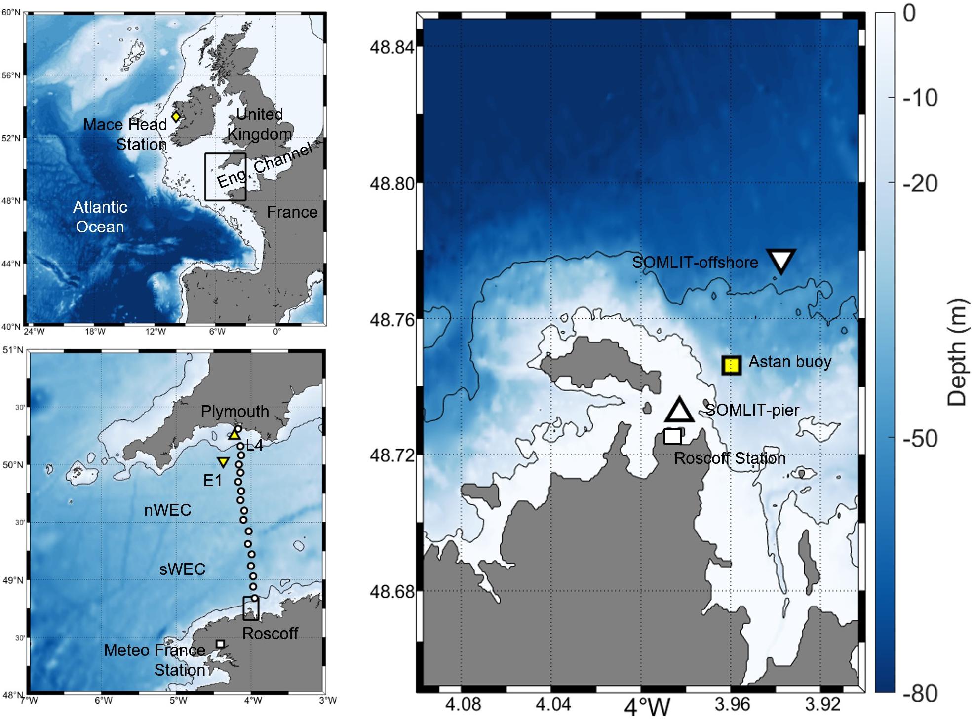
Figure 1. (Right) Map and bathymetry (5 and 50 m isobaths) of the study area in the sWEC with the location of the ASTAN buoy (yellow square) with the two SOMLIT sampling sites: SOMLIT-pier (upward triangle) and SOMLIT-offshore (downward triangle) and the location of the Roscoff observatory. (Top left) Map and bathymetry (200 m isobath) of the North Atlantic Ocean with the location of the Mace Head atmospheric station, the black frame represents the WEC. (Bottom left) Map and bathymetry (50 m isobath) of the WEC with the Meteo France station (white square) for wind speed data, E1 (downward triangle), L4 (upward triangle) and FerryBox transect from Roscoff to Plymouth used in the comparison of FCO₂ in Section “Dynamics of FCO₂ in the WEC” and Figure 10.

Two low-frequency stations are present either side of the HF buoy (Figure 1), with SOMLIT-pier located south of the buoy (48:43′59′′ N; 3:58′58′′ W) and SOMLIT-offshore located north (48:46′49′′ N; 3:58′14′′ W). Despite their close proximity, these two stations are quite different. SOMLIT-pier is located very close to the coast, strongly influenced by coastal waters, with a particular hydrodynamic regime: a strong tidal range and a low water column (around 5 m). SOMLIT-offshore is characteristic of sWEC surface waters with a well-mixed water column (around 60 m), with the distance from the coast (3.5 km) limiting the impact of rainwater and river inflow.

Materials and Methods

High-Frequency Measurements From the ASTAN Buoy

From 2015 to 2019, conductivity and temperature were recorded every 30 min using a SBE16 + (SeaBird, Inc.) instrument. A Cyclops7 fluorimeter (Turner Designs, Inc.) and a SBE43 sensor (Seabird, Inc.) measured at the same frequency Chl-a fluorescence and DO, respectively. The manufacturer accuracies were ± 0.005°C for the temperature sensor, 2% for oxygen saturation and 0.0005 S/m for conductivity. TBTO^® anti-fouling cylinders and black Tygon^® tubing were installed in the pumping circuit to prevent biofouling, which is a major issue for deployment of sensors in coastal water, with a critical period from May to September.

A Submersible Autonomous Moored Instrument for CO₂ (SAMI-CO₂, SunBurst Sensors) was installed from March 2015 to December 2019 to measure pCO₂ in seawater with a 1-h frequency. The SAMI-CO₂ sensor uses calibrated reagent-based colorimetry to measure the change in pH of the dye [bromothymol blue (BTB)]. The BTB is contained in a gas-permeable membrane that is exposed to the environment. The pH change is driven by diffusion of CO₂ across the membrane. The dye absorbance is recorded at two wavelengths, corresponding to the absorption peaks of acid/base forms of BTB. Blank measurements were performed regularly in distilled water for quality control. The accuracy of measurements reported by the manufacturer is ± 8 μatm (DeGrandpre et al., 1997). All sensors were recovered every 3 months for inspection, cleaning, battery checks and control of reagent levels.

Bimonthly Measurements at Fixed Stations SOMLIT-Pier and SOMLIT-Offshore

From March 2015 to December 2019, bimonthly sampling was performed at SOMLIT-pier and SOMLIT-offshore fixed stations (Figure 1) during neap tides and at high tide slack. CTD profiles were obtained with a Seabird SBE19 + with accuracies for temperature and computed salinity of 0.005°C and 0.002 respectively. Discrete seawater was sampled using 10 L Niskin bottle. Salinity measurements were performed by sampling seawater in glass bottles with a rubber seal and analyzed in the following months in a temperature regulated room with a portasal Guidline Salinometer at the SHOM (Service Hydrographique et Oceanographique de la Marine) with an accuracy of 0.002. For DO measurements seawater from the Niskin bottle was transferred into 280 mL brown glass bottles that were sealed with special caps to remove all air after addition of 1.7 mL of Winkler reagent I and II. Bottles were kept in the dark in a water bath and analyzed by the Winkler method using potentiometric end-point determination using a Metrohm titrator. The estimated accuracy of this method is 0.2 μM (Carpenter, 1965). For Chl-a measurements 500 ml of seawater were filtered through a GF/F (Whatman) glass filter under 0.2 bar vacuum. The filters were stored in a plastic tube at −20°C before analysis. The EPA (1997) extraction method was used in which Chl-a was extracted in a 90% acetone solution for a few hours at 4°C, followed by measurement of Chl-a concentration using a Turner AU10 fluorometer. Nutrient concentrations (${\text{PO}}_4^{3-}$ and SiO₄^–) were determined using an AA3 auto-analyzer (AXFLOW) following the method of Aminot and Kérouel (2007) with accuracies of 1 ng L^–1 and 0.01 μg L^–1 for ${\text{PO}}_4^{3-}$ and SiO₄^–, respectively. During the same period, total alkalinity (TA), dissolved inorganic carbon (DIC) and pH were measured at SOMLIT-pier and SOMLIT-offshore stations. Seawater was sampled in 500 mL borosilicate glass bottles and poisoned with 50 μL of saturated HgCl₂. TA and the DIC were determined at the SNAPO (Service National d’Analyse des Paramètres Océaniques) using potentiometric analysis following the Edmond (1970) method and DOE (1994) with accuracies of 2.5 μmol kg^–1 for both parameters (see Marrec et al., 2013 for details on this method). pH was determined using the same protocol as for the ASTAN buoy measurements (see below).

From March 2017 to December 2019, additional sampling for pH and TA in the vicinity of the ASTAN buoy was performed every 2 weeks. 50 discrete samples for the determination of TA and pH were collected in 500 mL borosilicate glass bottles and poisoned with 50 μL of saturated HgCl₂. TA was determined from approximately 51 g of weighed sample at 25°C using a potentiometric titration with 0.1M HCl using a Titrino 847 plus Metrohm. The balance point was determined by the Gran method (Gran, 1952) according to the method of Haraldsson et al. (1997). The accuracy of this method is ± 2.1 μmol kg^–1 (Millero, 2007) and was verified by Certified Reference Material (CRM 131) provided by A. Dickson (Scripps Institute of Oceanography, University of South California, San Diego, United States). pH was determined with an accuracy of 0.002 pH units by spectrophotometry (Perin-Elmer Lambda 11) at a controlled temperature of 25°C with the method of Clayton and Byrne (1993) and corrected by Chierici et al. (1999), using the sulfonephthaleindiprotic indicator of meta-CresolPurple (mCP).

Calculated Data

Dissolved Oxygen Saturation

Calculation of dissolved oxygen saturation (DO%) gives access to the impact of non-thermodynamical processes, such as biological production and respiration, on the variation of DO. The DO% was calculated from Eq. 1 using in situ temperature, salinity, and dissolved oxygen concentrations.

$$\begin{array}{c}\hfill In{C}^{*}=A_1+(\frac{A_2\times T}{100})+[A_3\times \log (\frac{T}{100})]\hfill \\ \hfill +S\times [(B_1+(B_2\times \frac{T}{100})+B_3\times {(\frac{T}{100})}^2)]\hfill \\ \hfill DO\%=(\frac{DO}{C^{*}})\times 100\hfill \end{array}(1)$$

Where C^∗ is the concentration of DO at saturation, A and B coefficients are constants described in Weiss (1970), T is the SST (in K) and S the sea surface salinity (SSS).

Carbonate System Parameters

At the ASTAN buoy, we used the combination of TA, pH, SSS and SST as input parameters in the CO₂ chemical speciation model (CO_2sys Program, Pierrot et al., 2011). We used the equilibrium constants of CO₂ proposed by Mehrbach et al. (1973), refitted by Dickson and Millero (1987) on the total pH scale, as recommended by Dickson et al. (2007) and Orr et al. (2015), and including ${\text{PO}}_4^{3-}$ and SiO₄^– concentrations. At SOMLIT-pier and SOMLIT-offshore, from January 2015 to April 2018, we used the combination of TA, DIC, SSS, SST, ${\text{PO}}_4^{3-}$ and SiO₄^– concentrations, and from May 2018 to December 2019 we used the combination of pH, DIC, SSS, SST and ${\text{PO}}_4^{3-}$ and SiO₄^– concentrations as input parameters in the model. We use the standard uncertainty propagation package updated by Orr et al. (2018) for comparison with current computations of uncertainty on the carbonate system parameters in the field of OA. The average uncertainty on pCO_2calc were estimated at 11 μatm for TA/pH, at 18 μatm for DIC/TA and at 8 μatm for pH/DIC. These uncertainties were in agreement with similar pCO_2calc computations using the propagation technique: 20 μatm for Shadwick et al. (2019) and 15 μatm for Kapsenberg et al. (2017) with DIC/TA as entry parameters.

To estimate pH variations from pCO₂ at the ASTAN buoy (pH_calc), we relied on 20 seasonal surveys performed in 2011, 2019 and 2020, when we collected more than 150 data points for TA and SSS covering the entire SSS gradient (0–35.5) in the Penzé and Morlaix rivers, the main sources of freshwater input at our study site. We combined these data with the 2016 discrete dataset marked by intense freshwater inputs at the ASTAN site with important rainfall (563 mm during that winter compared to 274 mm during 2019), and SSS varying from 34.50 to 35.50. We were able to establish a very robust relationship between TA and SSS (n = 236, r² = 0.98) with the following equation 2 (Supplementary Figure S1):

$$TA{}_{calc}=50.4{(\pm 0.5)}^{*}SSS+575(\pm 14)\mathit{\hspace{1em}\hspace{1em}\hspace{0.5em}\hspace{0.25em}}(2)$$

We therefore estimated the HF pH with CO_2sys using the same parameters SST, SSS, pCO₂ and TA_calc. We compared the discrete pH values obtained in 2019 at the ASTAN buoy with the spectrophotometric technique [precision of 0.001 and bias of 0.005 pH units (Dickson et al., 2007)] to the pH_calc from the TA/SSS relationship (Supplementary Figure S2). From this comparison, we estimate the uncertainty on the pH_calc at 0.04.

Deconvolution of Thermal and Non-thermal Processes on pCO₂

The variability of surface pCO₂ caused by thermal and non-thermal processes was estimated from Takahashi et al. (1993, 2002). The method is based on the well-constrained temperature dependence of pCO₂ (4.23%°C^–1) (Takahashi et al., 1993). It helps to construct the thermally forced seasonal pCO₂ cycle (pCO₂^therm, Eq. 3) and remove the thermal effect from observed pCO₂ (pCO₂^non–therm, Eq. 4). We then were able to quantified the respective influence of δpCO₂^therm (pCO₂-pCO₂^non–therm) and δpCO₂^non–therm (pCO₂-pCO₂^therm) on the pCO₂.

$$pC{O}_2^{therm}=pC{O}_{2,mean}\times e^{0.0423\times (T_{obs}-T_{mean})}\mathit{\hspace{1em}\hspace{1em}}(3)$$

$$pC{O}_2^{non-therm}=pC{O}_{2,obs}\times e^{0.0423\times (T_{mean}-T_{obs})}\mathit{\hspace{1em}\hspace{1em}}(4)$$

For HF data from the buoy, pCO_2,obs and T_obs are the calibrated pCO₂ data (Figure 2 and Supplementary Figure S2) from the SAMI-CO₂ and the SST measured at ASTAN, respectively. pCO_2,mean is the mean sea surface pCO₂ (420 ± 50 μatm, n = 30788) and T_mean the annual average temperature (13.20 ± 2.09°C, n = 33442), calculated from the most complete HF dataset recorded in 2016 and 2019 (Supplementary Table T1). For bimonthly data, means were calculated from January 2015 to December 2019 based on the bimonthly dataset: pCO_2,obs is the pCO₂ computed from TA/DIC and pH/DIC, with an annual mean of pCO_2,mean = 410 ± 64 μatm (n = 109) at SOMLIT-pier and pCO_2,mean = 436 ± 39 μatm (n = 119) at SOMLIT-offshore. The average temperature observed at SOMLIT-pier was T_mean = 13.17 ± 2.27°C (n = 119) and at SOMLIT-offshore was T_mean = 13.05 ± 2.04°C (n = 121) (Supplementary Table T1).

FIGURE 2

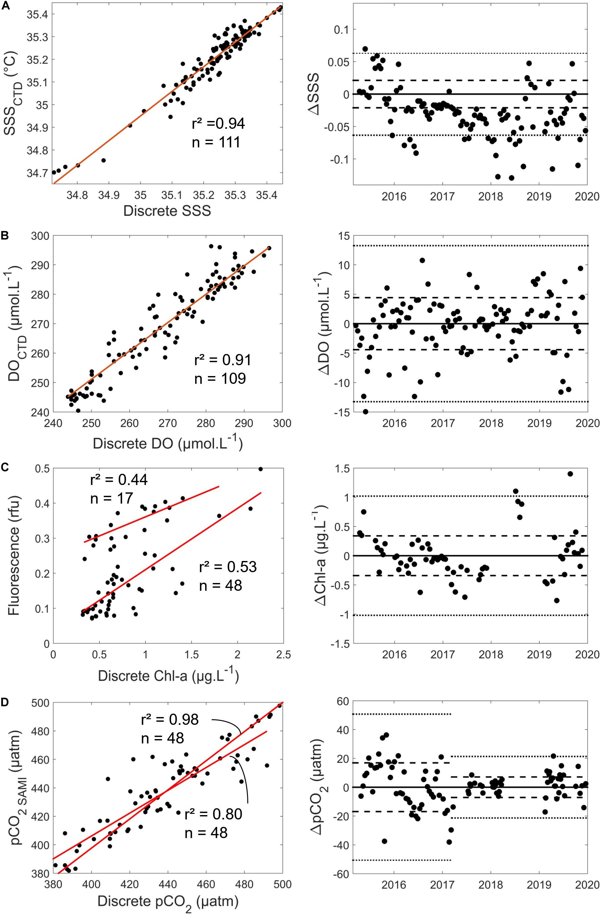
Figure 2. Correlations between HF and discrete data for (A) SSS, (B) DO (μM), (C) Chl-a (μg L^–1), and (D) pCO₂ (μatm). Left plots show discrete measurements versus sensor values, with n the number of discrete measurements, red lines the linear regression between discrete and sensor measurements and associated r² values. The right plot shows the differences between sensor values and discrete measurements over time. Dashed lines represent standard deviation of the difference between sensor values and discrete measurements, and dotted lines represent three times the standard deviation.

Air-Sea CO₂ Fluxes

Atmospheric pCO₂ (pCO₂^air) was calculated from the CO₂ molar fraction (xCO₂) from the Mace Head site (53°33′ N 9°00′ W, southern Ireland) (Figure 1) of the RAMCES network (Observatory Network for Greenhouse gases) and from the water vapor pressure (pH₂O) using the Weiss and Price (1980) equation. Atmospheric pressure (P_atm) was obtained from the weather station of the Roscoff Marine Station, and the wind data from the Guipavas meteorological station (48°26′36′′ N, 4°24′42′′ W, Météo France) (Figure 1). All data were recorded at hourly frequency and then allocated to the HF pCO₂ signal of the ASTAN buoy obtained every 30 min by linear interpolation, daily means were then assigned to discrete values of SOMLIT stations. FCO₂ (in mmol C m^–2 d^–1, Eq. 5) at the air-sea interface was determined from the difference of pCO₂ between the surface seawater and the air (δpCO₂ = pCO₂-pCO₂ ^air), SST, SSS and wind speed.

$$FC{O}_2=k\times \mathrm{\alpha }\times \mathrm{\delta }pC{O}_2\mathit{\hspace{1em}\hspace{1em}\hspace{1em}\hspace{0.5em} }(5)$$

Where k represents the gas transfer velocity (m s^–1) and α represents the solubility coefficient of CO₂ (mol atm^–1 m^–3) calculated as in Weiss (1970). The exchange coefficient k (Eq. 6) was calculated according to the wind speed with the updated algorithm of Wanninkhof (2014) appropriate for regional to global flux estimates and high spatial and temporal resolution of wind products:

$$k=0.251\times u_{10}^2\times {(\frac{Sc}{660})}^{-0.5}\mathit{\hspace{1em}\hspace{1em}\hspace{1em}\hspace{0.5em} }(6)$$

Where u₁₀ represents the wind speed at 10 m height (m s^–1) and S_c the Schmidt number at in situ surface temperature, which varied from 770 to 1250.

Wavelet Analysis

To extract further information on our HF data, mathematical transformations were applied. In 2016 and 2019 the HF dataset covered a major part of the year, and all the studied parameters were measured simultaneously. Wavelet analyses were thus performed on SST, SSS, DO%, and pCO₂^non–therm to identify the principal frequencies driving the variability of these parameters. Typically, Fourier transforms are used to quantify the constant periodic component in time series. This method is limited when the frequency content changes with time, as in the case of ecological time-series. To overcome these limitations, the wavelets analysis became the norm in environmental time-series analysis, and were used for example to analyze El Nino Southern oscillation (Goring and Bell, 1999) or to follow precipitations distributions (Santos and de Morais, 2013). Wavelet analysis maintain time and frequency localization in a signal analysis, decomposing a time-series into a time-frequency image. This image, generated as a power spectrum, provides simultaneous information on the amplitude of any periodic signals within the series, and on how this amplitude varies with time (Santos and de Morais, 2013). Our measurements were carried out at stations influenced by many factors, stationary or not (e.g., tidal range, currents, day–night cycle, marked seasons…). In the case of such HF analysis of an environmental signal the continuous wavelet transform (CWT) must be used and the Morlet wavelets are privileged to follow localized scales (Cazelles et al., 2008). The wavelets analysis is also suitable for the analysis of the relationship between two signals, and thus determining the links between each of the environmental variables studied. We used the cross-wavelets transforms to estimate the covariance between each pair of time-series as a function of frequency. The wavelet analyses were carried out from the Matlab package “wavelet-coherence” (Grinsted et al., 2004) on Matlab v2015b.

Results

Reliability of the Dataset

From the 06/03/2015 to the 31/12/2019, SST from the Seabird SBE16 + of the ASTAN buoy and from SBE19 + used during discrete sampling at SOMLIT-offshore were very well-correlated (r² = 0.99, n = 99, standard deviation of the residuals < 0.1°C) (Supplementary Figure S3). We used the bimonthly discrete measurements of SSS, DO and Chl-a from the SOMLIT-offshore station to determine whether post-calibration of the corresponding sensors of the SBE16 + deployed at the ASTAN buoy was necessary. These samples were collected during high tide slack when the ASTAN and SOMLIT-offshore surface waters had similar biogeochemical properties according to our transect data. The SSS values were in good agreement with discrete salinity measurements with a 1:1 relationship (r² = 0.95, n = 111; standard deviation of the residuals < 0.02) (Figure 2A). Similarly, for DO the linear relationship between both measurements was close to 1:1 (DO = 1.03*DO_SBE43−6.7, r² = 0.91, n = 109, standard deviation of the residuals < 4.4 μM) (Figure 2B). During the 5 years of study, the mean difference between discrete DO and DO measured by the SBE43 sensor was 0.31 μM. In light of these results, no corrections were applied to the HF SSS and DO. For Chl a two different fluorometers were used during the study, from March 2015 to June 2018 and from June 2018 to December 2019. During the first and second deployments, fluorescence (in relative fluorescence units, RFU) showed significant correlations with discrete Chl-a concentrations of (1) Fluorescence = 0.18^∗Chl-a + 0.04, r² = 0.52, n = 48 and (2) Fluorescence = 0.11^∗Chl-a + 0.25, r² = 0.43, n = 17, respectively (Figure 2C). Once the two different conversions between fluorescence and Chl-a measurements were performed, the standard deviation on the residuals was 0.34 μg L^–1. Conversion of in situ fluorescence into Chl-a concentrations has always been challenging, with fluorescence influenced by numerous factors: heterogeneity of the phytoplankton community structure across the year (Southward et al., 2005; Guilloux et al., 2013), phytoplankton taxonomy (Proctor and Roesler, 2010), cell size (Alpine and Cloern, 1985), pigment packing (Bricaud et al., 1983, 1995; Sosik et al., 1989; Sosik and Mitchell, 1991) and the effect of non-photochemical quenching (Xing et al., 2012). Despite these limitations, Chl-a concentrations remains a suitable proxy for phytoplankton biomass (Carberry et al., 2019). The standard deviations obtained on the residuals were close to those obtained with similar sensors on the Armorique Ferry Box between Roscoff and Plymouth (Marrec et al., 2014), therefore no further corrections were applied to the converted Chl a signal.

Maintenance of the SAMI-pCO₂ sensor was conducted at least every 3 months and more often during the productive period. Offsets between discrete pCO₂ estimates and SAMI-pCO₂ were detected each time. The offset remained stable during the deployment periods. For example, from the 13/07/2017 to the 31/08/2017, the mean difference between discrete measurements and the sensor was + 8.9 μatm, while from 02/10/2017 to 11/01/2018 it was −9.9 μatm. The pCO₂ values obtained from the sensor were corrected using measured offsets. From March 2015 to March 2017, we used the TA/DIC measurements at SOMLIT-offshore during high tide slack to compute pCO₂. The pCO₂ values obtained from the sensor were corrected from the measured offset, taking into account the average difference between SOMLIT-offshore and ASTAN buoy. Once the offset was corrected (Figure 2D), we obtained a 1:1 relationship between in situ pCO₂ computed from DIC/TA and pCO₂ values given by the SAMI-CO₂ (r² = 0.80, n = 48) with a standard deviation of the residuals of 16.9 μatm. From March 2017 to December 2019, to reduce errors linked to short time and space scales variability, discrete samples for the determination of pH and TA were taken very close to or directly from the buoy at the same depth than the SAMI sensor. We used this pH/TA combination to compute sea surface pCO₂ at the buoy since they provide accurate pCO₂ values (Millero, 2007). We obtained a better 1:1 relationship between in situ pCO₂ computed from pH and TA and pCO₂ values given by the SAMI-CO₂ (r² = 0.98, n = 48) with a standard deviation of the residuals of 7.1 μatm.

The percentage of environmental parameters acquired by each sensor had a mean success rate of 60% (Table 1). The SST and SSS mean ratios were most reliable due to the robustness of these sensors. SSTs measured concomitantly by the CTD and the SAMI-CO₂, were well-correlated (Supplementary Figure S3B). DO and fluorescence sensors were more sensitive to specific problems (e.g., biofouling) due to the substantial sensitivity of detection technologies used by theses sensors, which are based on polarography (SBE43) and optics (Cyclops C7), respectively. The SAMI-CO₂ was the most impacted sensor in terms of acquisition, principally due to frequent battery shortage, missing reagents, or problems with embedded electronics. With the installation of radio transmission during summer 2018, it was easier to detect breakdowns and therefore quickly undertake repairs. The percentage of data acquisition thus increased for all sensors from this point onwards.

TABLE 1

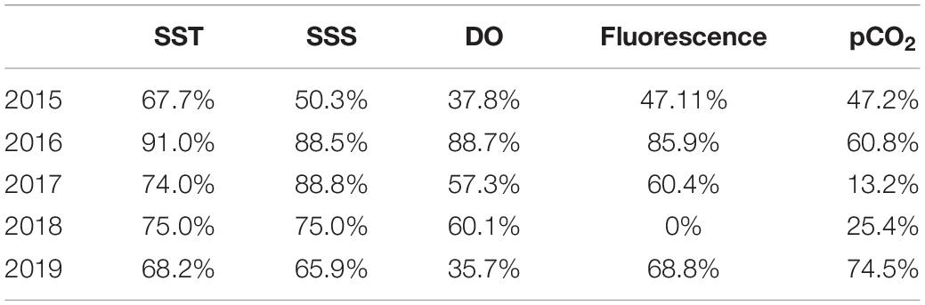
Table 1. Percentage of data acquired for each parameter measured at the ASTAN buoy from March 2015 to December 2019.

Physical and Biogeochemical Variability of Coastal sWEC Waters

Variability of Physical Parameters

Sea surface temperature and SSS showed marked seasonality with cold and fresh water during winter and early spring, and warmer and more saline waters during summer and early fall (Figures 3A,B). SST ranged from 9.0°C during winter to 17.0°C during summer. Averaged seasonal SST at SOMLIT-pier was warmer than at SOMLIT-offshore during summer (15.89 ± 0.70°C, n = 31 vs. 15.34 ± 0.66°C, n = 31, p-value < 0.001), and colder during winter (10.44 ± 0.78°C, n = 36 vs. 10.75 ± 0.76°C, n = 37, p-value < 0.001) (Supplementary Table T1). The seasonal mean of SSS varied from ∼35.15 ± 0.13 in winter to ∼35.27 ± 0.13 in summer. SSS at SOMLIT-pier was significantly lower than at SOMLIT-offshore because of larger freshwater inputs during the winter with a mean difference of 0.30 (Supplementary Table T1). During summer SSS at both stations was in a similar range. At the ASTAN buoy, high-frequency SSS measurements indicated a variability of up to 0.70 within 24 h cycles in winter and up to 0.30 during summer. Interannually, the climatology was calculated from HF daily means of SST and SSS values over 5 years and SST followed a similar pattern between years, except in winter 2018 when the coldest SST was observed, with a 1.5°C difference compared to the 5-year average. SSS did not follow regular seasonality: in 2015 and 2017 SSS followed the 5-year average, with SSS values remaining above 35.0; while in 2016 and 2018, winter SSS decreased down to 34.80 and 34.50, respectively (Figure 3B).

FIGURE 3

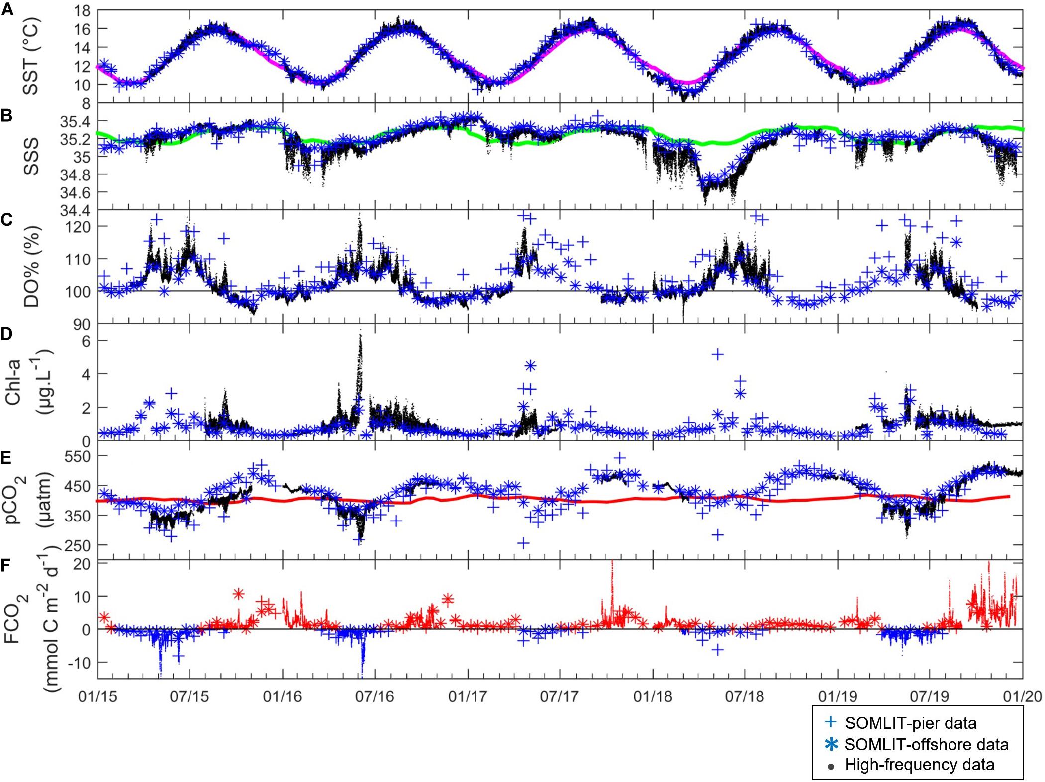
Figure 3. (. in black) High-frequency, (+ in blue) SOMLIT-pier, and (* in blue) SOMLIT-offshore data of (A) SST (°C), (B) SSS, (C) DO% (%), (D) Chl-a (μg L^–1), (E) pCO₂ (μatm) and (F) FCO₂ (mmol C m^–2 d^–1) from January 2015 to January 2020. Colored lines represent the climatology of (A) SST, (B) SSS, and the pCO₂^atm (μatm) on (E). The black lines of (C,F) represent the atmospheric equilibrium of DO and CO₂, respectively. Negative FCO₂ (sink of atmospheric CO₂) values are represented in blue, and positive FCO₂ (source of CO₂ to the atmosphere) are in red.

Variability of Chl-a Concentrations and DO%

The SOMLIT-pier DO% and Chl-a were higher than SOMLIT-offshore values, with a mean difference around 2% and 0.05 μg L^–1 in winter, and around 10% and 0.1 μg L^–1 in summer. At ASTAN, the variations of HF DO% and converted Chl-a showed similar dynamics with high DO% > 110%, high Chl-a concentrations (>2 μg L^–1) during spring, and low Chl-a (<0.5 μg L^–1) concentrations associated with low DO values close to the equilibrium and/or undersaturated during fall/winter with a mean DO% of 98.2 ± 1.6% during winter and values below 93% in November (Figures 3C,D and Supplementary Table T1). The DO oversaturation generally lasted around 6 months, from April to September, and surface waters were close to equilibrium and/or undersaturated in DO for the rest of the year. High-frequency DO% data recorded at the ASTAN buoy were closer to the data observed at SOMLIT-offshore than at SOMLIT-pier. Both DO% and Chl-a were characterized by high variability when observed from HF measurements, particularly during spring and summer. DO% and Chl-a followed the same general pattern each year but differed temporally. For example DO oversaturation (DO% above 115%) and high Chl-a (5 μg L^–1) were observed in early spring (March) during 2015, but only during late spring (May) in 2018 (Figures 3C,D), when large riverine inputs marked by lower SSS values occurred.

Variability of pCO₂ and FCO₂

At SOMLIT-offshore and SOMLIT-pier, pCO₂ ranged from 295 to 507 μatm on an annual scale (Figure 3E). Minimum values (<350 μatm) were observed during spring and early summer, with pCO₂ values below atmospheric equilibrium (pCO₂^air ranging from 400 to 410 μatm). Maximum values (>450 μatm), above atmospheric equilibrium, were observed during fall and early winter (Figure 3E). Surface water CO₂ undersaturation relative to pCO₂^air lasted around 6 months, from April to September, while CO₂ oversaturation dominated the rest of the year, inversely related to DO%. During summer, pCO₂ at SOMLIT-offshore was higher than at the SOMLIT-pier (+ 65 μatm mean difference), while during winter we observed an opposite pattern (−23 μatm mean difference). HF pCO₂ was generally well-correlated to the low frequency data. However, during May 2016 and 2019 HF data indicated important drawdowns below 300 μatm (related to high Chl a values), which were not detected by the low frequency monitoring.

The annual amplitude of FCO₂ (Figure 3F) varied from −14 mmol C m^–2 d^–1 to + 26 mmol C m^–2 d^–1. During winter, the fluxes were positive, with surface waters releasing CO₂ to the atmosphere, while the spring negative values revealed a strong absorption of atmospheric CO₂. During spring, atmospheric CO₂ absorption at the SOMLIT-pier was larger (−2.10 ± 1.80 mmol C m^–2 d^–1, n = 29) than at SOMLIT-offshore (0.29 ± 1.00 mmol C m^–2 d^–1, n = 31), with an average difference of 1.8 mmol C m^–2 d^–1 (Supplementary Table T1). During winter, the two stations acted rather similarly, with important CO₂ emissions to the atmosphere during the high wind speed periods (e.g., December 2015 and January 2018) (Figure 3F). The HF monitoring enabled the observation of important daily FCO₂ variations during the spring of 2015 and 2016. For example, during 2015 HF data revealed values down to −14 mmol C m^–2 d^–1, compared to the FCO₂ computed from discrete sampling around −4 mmol C m^–2 d^–1. Similar observations were made during winter 2015, 2016, 2017 and 2019 with, as in 2017, high HF FCO₂ values of 26 mmol C m^–2 d^–1 compared to values of 3 mmol C m^–2 d^–1 computed from discrete sampling at the same time. Mean seasonal FCO₂ were relatively similar at the three stations during winter, with values between + 2.0 and +4.0 mmol C d^–2 m^–1 (Figure 4). The spatial difference was more marked during spring, when FCO₂ was negative at SOMLIT-pier (less than −2 mmol C m^–2 d^–1) and at ASTAN buoy (around −1.6 mmol C m^–2 d^–1), but close to equilibrium at SOMLIT-offshore (around −0.3 mmol C m^–2 d^–1). During summer, SOMLIT-pier and ASTAN buoy had values close to atmospheric equilibrium, while SOMLIT-offshore surface waters released CO₂ at + 1.0 mmol C m^–2 d^–1. During fall, all sites exhibited large emissions of CO₂ to the atmosphere with values between + 2 and + 6 mmol C m^–2 d^–1.

FIGURE 4

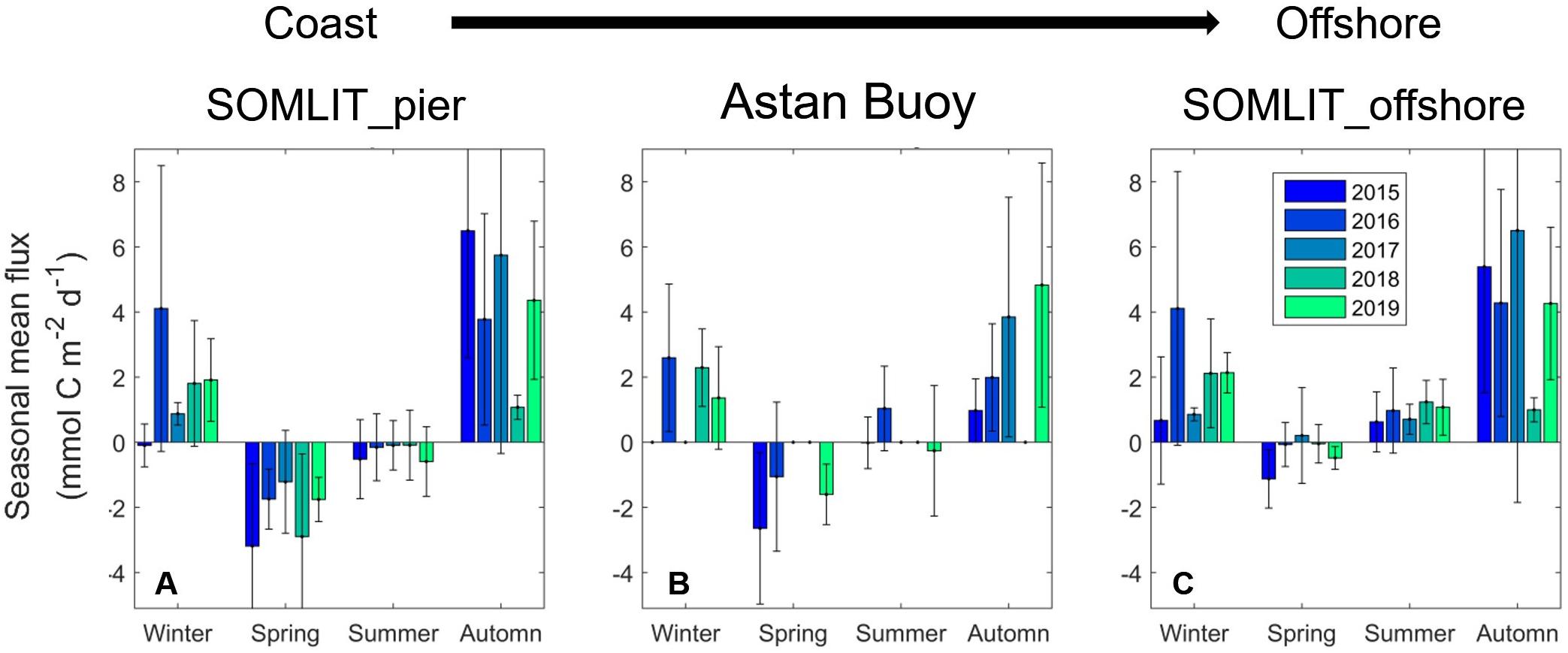
Figure 4. Seasonal mean FCO₂ (mmol C m^–2 d^–1) across a coast-to-offshore gradient at (A) SOMLIT-pier (B) ASTAN buoy, and (C) SOMLIT-offshore from 2015 to 2019. The high frequency means were established only for seasons with a number of observations n_obs > 1500, and for the bimonthly stations with a n_obs > 4. The error lines represent the standard deviation.

Frequency Analysis

Frequency Study of the Physical Structure

Wavelet analyses were applied to the 2016 and 2019 HF SST and SSS data (Figure 5A) to identify the main frequencies of variability at the ASTAN buoy. The years 2016 and 2019 were used because the datasets were the most complete. For both years, the SST followed closely the climatology, while the SSS signal was more variable each year because of the high riverine variability but did not show extreme values as those recorded in 2018.

FIGURE 5

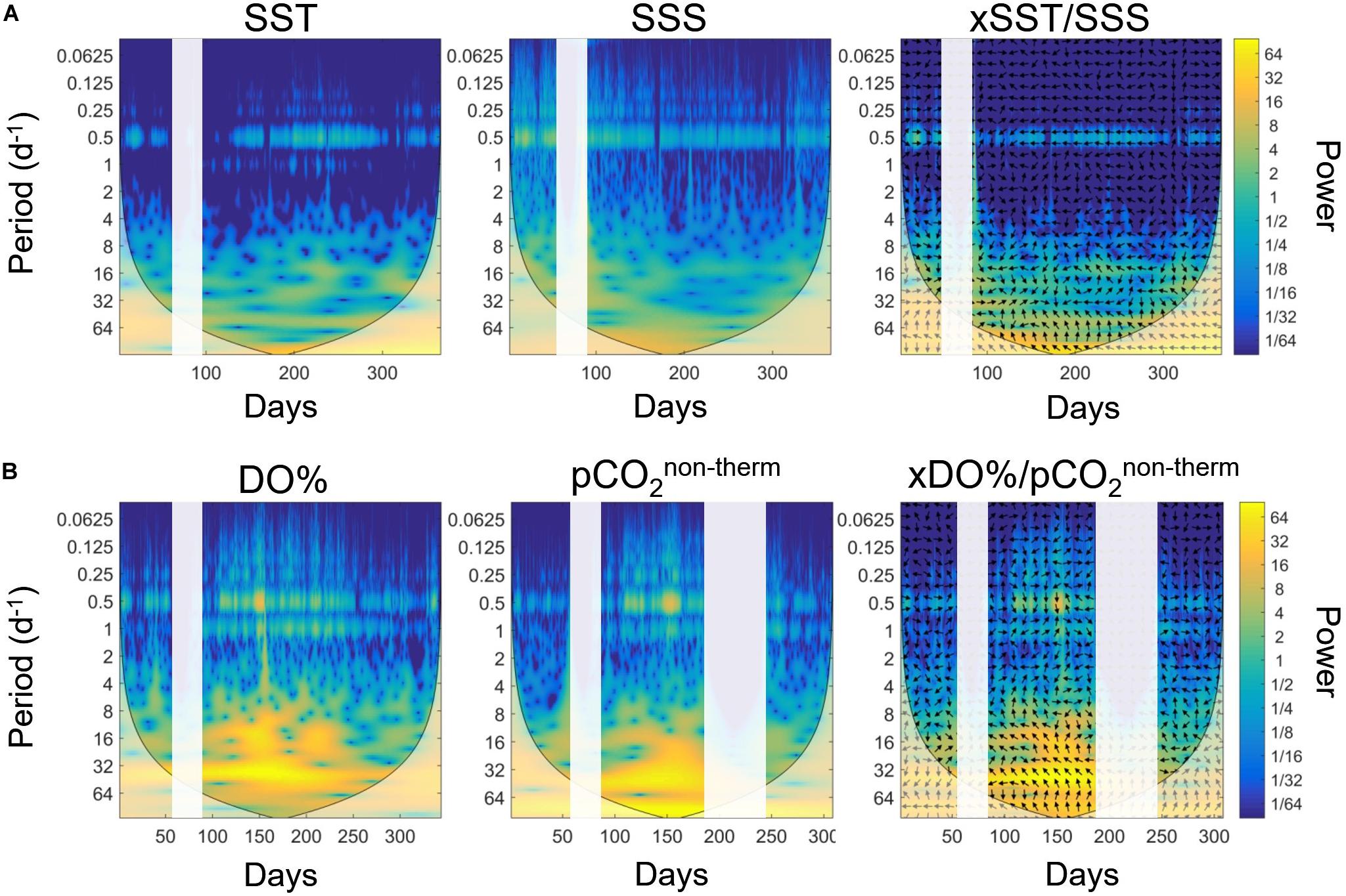
Figure 5. Wavelet power spectrum based on the Morlet wavelets during the year 2016 for (A) SST (°C), SSS, and cross-wavelet spectrum between SST and SSS, and for (B) DO% (%), pCO₂^non–therm (μatm) and cross-wavelet spectrum between DO% and pCO₂^non–therm. Time is expressed in day of the year. The color bars represent the power of the wavelet transform, in absolute squared value. A high power is represented in yellow. For the cross-wavelets spectrum, the arrows indicate if the signals are in phases (arrow pointing right) or in phase inversion (arrow pointing left). White bands represent a lack of data.

A 12 h cycle, representative of the tidal period of 0.5 day, clearly appeared on both wavelet analyses throughout the year: high variance values between the signal and the wavelets appeared, indicating more marked correlations during the summer period for SST and during winter for SSS. The diurnal cycle (period of 1 day) appeared weakly and episodically in the wavelet transformation of SST data. The crossed wavelets of SST and SSS highlighted the main periodicity of 0.5 days. At the 12 h frequency, we clearly observed a phase alternation, represented by the change of direction of the arrow, with a signal in phase from October to April, and shifted the rest of the year. The statistical analysis revealed very sharp phase changes and allowed precise pinpointing of the different physical characteristics of two water masses influencing HF measurements. For example, the first inversion started on April 10 during 2016, while the second inversion occurred on November 9 in 2016. Similar analysis for 2019 revealed an inversion on November 7 in 2019, remarkably close in terms of inter-annual variability. These results underline the potential of HF monitoring combined to wavelet analyses for following shifts in terms of physical regimes in complex nearshore ecosystems.

Frequency Study of Biogeochemical Parameters

Wavelet transformation for the biogeochemical parameters DO% and pCO₂^non–therm (Figure 5B), representative of biological processes, revealed two characteristic frequencies of 0.5 and 1 days. These frequencies were more marked during summer compared to winter, with higher power. The cross-wavelet analysis revealed that these two frequencies were identical for both parameters underlying potential diel biological cycles in surface waters at the ASTAN buoy. However, the phases did not show any relevant pattern, and the cross wavelet between the biological and the physical parameters didn’t bring more information (not shown). For the 12 h signal, we did not observe distinct regimes similar to those of SST and SSS. In winter, they seemed shifted, with DO% maximal when pCO₂^non–therm decreased.

Short-Term Variability of Physical and Biogeochemical Parameters

Short-term variability of HF data recorded at the ASTAN buoy during two representatives 6-days periods in January 2016 and May 2016 is shown in Figure 6. From 05/01/2016 to 10/01/2016 (winter period, Figure 6A), SST ranged from 11 to 14°C, and SSS from 34.85 to 34.95. The SST and SSS varied following 12-h cycles: SST and SSS differences within a 6-h time frame ranged from 0.10 to 0.30°C for SST and from 0.03 to 0.40 for SSS. These two parameters followed the same pattern as the tidal ranges. During high tides SST and SSS reached their highest values, while during low tides minimum SST and SSS values were observed. Similarly, 6-h variation was observed for DO and pCO₂ (Figure 6C). DO ranged from 264 to 274 μM, and pCO₂ ranged from 443 to 457 μatm with a 6-h difference of around 7 μM and 13 μatm, respectively.

FIGURE 6

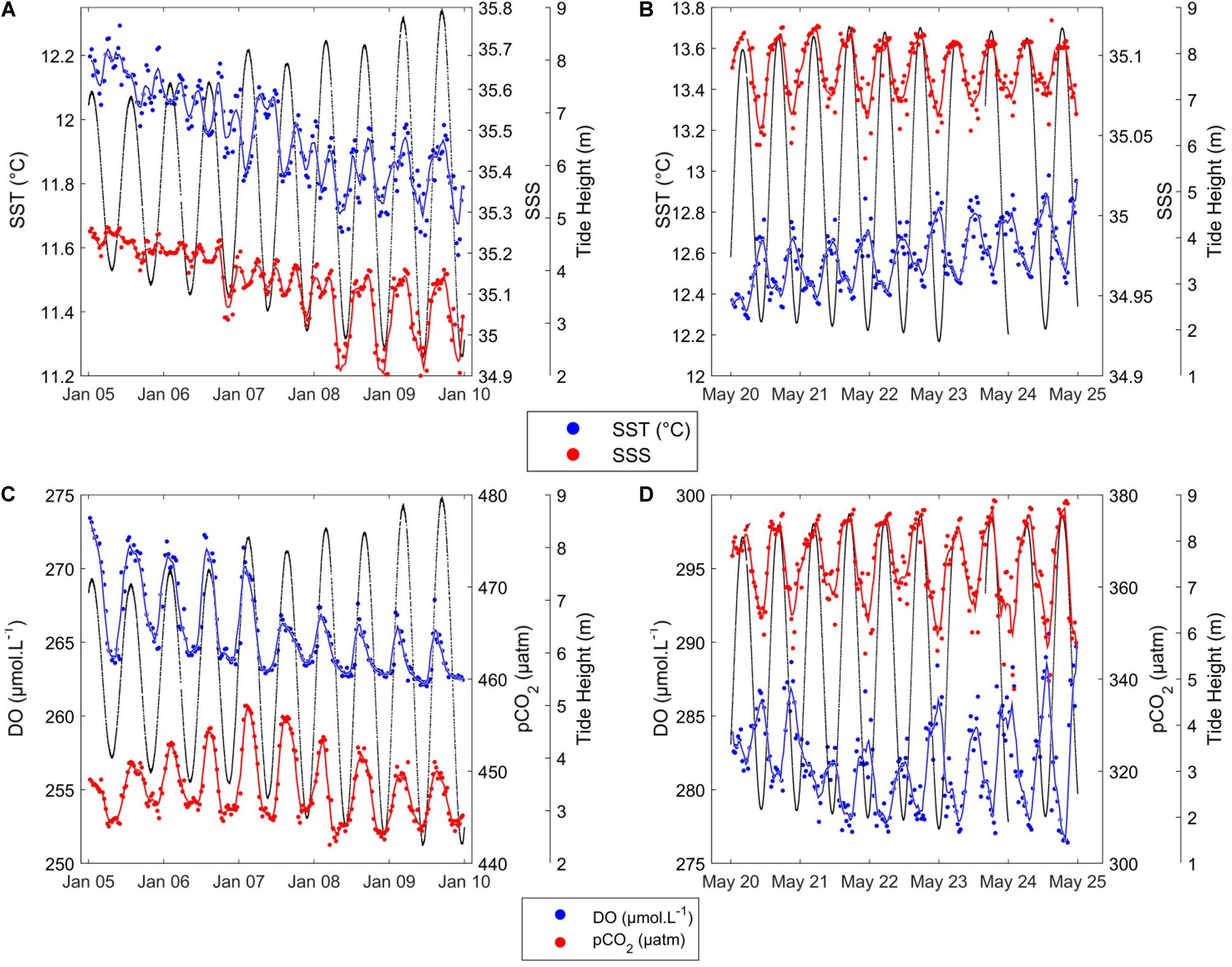
Figure 6. Short-term variability of SST (°C) (blue) and SSS (red) during (A) winter, from 05/01/2016 to 10/01/2016, and (B) summer, from 20/05/2016 to 25/05/2016; and short-term variability of DO (μM) (blue) and pCO₂ (μatm) (red) during (C) winter and (D) summer. Black lines represent tidal height (m). Smooth lines in blue and red are obtained using a moving average filter with a 2-h span on the corresponding parameters.

From 20/05/2016 to 25/05/2016 (spring period, Figure 6B), SST ranged from 15.80 to 17.20°C, and SSS from 35.18 to 35.25. We observed 6-h variations of SST around 0.40°C, and 6-h variations of SSS around 0.50. SSS followed the tidal variations, and SST was in the opposite phase; i.e., the phase shift highlighted by the wavelet analysis had occurred. DO and pCO₂ patterns were linked to the 12 h tidal cycle, as suggested by the wavelet analysis. During the bloom (Figure 6D), DO ranged from 277 to 290 μM, and pCO₂ from 347 to 379 μatm. 6-h variations were 8 μM for DO and 20 μatm for pCO₂. pCO₂ was correlated with the tidal pattern, while DO was in the opposite phase. These observations highlight the importance of the tidal cycle in daily variations of biogeochemical parameters at the ASTAN buoy.

Discussion

Short-Scale Variability of the CO₂ System in Coastal sWEC

Discrete data, wavelet analysis and HF data described in Section “Short-Term Variability of Physical and Biogeochemical Parameters” highlighted the tidal transport of two distinct water masses: firstly a coastal water mass (CWM), unidentified in previous studies (Marrec, 2014), with properties corresponding to the SOMLIT-pier data and present at ASTAN during low tides; secondly an offshore water mass (OWM) corresponding to SOMLIT-offshore data and present at ASTAN during high tides. During the 5 years of observations, the CWM had lower SST during winter, higher SST during summer; and generally lower SSS (Figures 3A,B) (Supplementary Table T1) than the OWM. The phase inversion observed in November and April (Figure 5), which occurred every year, was the consequence of the opposite SST seasonality between the CWM and the OWM (lower SST in summer in OWM and lower SST in winter in CWM). The influence of tides on pCO₂ dynamics is prominent in estuarine ecosystems (De la Paz et al., 2007; Bozec et al., 2012; Oliveira et al., 2018), but has also been observed in various continental shelves of the world ocean (DeGrandpre et al., 1998; Hofmann et al., 2011; Horwitz et al., 2019). Several studies have reported the impact of the tidal cycle on pCO₂ over various European continental shelf provinces, for example in the nWEC (Litt et al., 2010), in the Bay of Brest (Bozec et al., 2011) or in the Cadiz Bay (Ribas-Ribas et al., 2011, 2013). Likewise, enhanced variability at 12-h periods of DO% and pCO₂ were associated to tidal levels and SST/SSS variations at ASTAN (Figures 5, 6). Previous studies were limited to shorter periods of observation, spanning from 20 h to 4 months, with tidal amplitude lesser than 2 m (Litt et al., 2010; Ribas-Ribas et al., 2011, 2013) or to a semi-enclosed bay with limited tidal exchange with the adjacent open ocean (Bozec et al., 2011). During 5 years, we observed mean variations of DO% and pCO₂ around 10% and 15 μatm, respectively, during tidal cycles. The maximum tidal variability associated to spring tides (>7 m) during phytoplankton blooms (16% for DO% and 88 μatm for pCO₂^non–therm) represented up to 50 and 40% of the respective annual signals at ASTAN. These variabilities reflected the important tidal transport of the CWM and OWM in the coastal sWEC, distinctively revealed by HF monitoring at the ASTAN buoy.

In addition to the tidal variability of DO% and pCO₂ as a result of the presence of distinct water masses at ASTAN, HF monitoring of these biologically dependent variables should also present diurnal variability. During the day, the combination of photosynthesis and respiration is supposed to increase DO% and decrease pCO₂^non–therm, whereas during the night, respiration processes tend to decrease DO% and increase pCO₂^non–therm. Borges and Frankignoulle (2003) first revealed a combination of the tidal signal coupled with the biological diel cycle on pCO₂ variations in the English Channel. The impact of the diel cycle on DO%, pCO₂^non–therm and FCO₂ had also been detected and quantified during the productive period in the nWEC (Marrec et al., 2014). In the adjacent Bay of Brest, HF data showed a maximum of DO% and a minimum of pCO₂ at dusk, and a maximum of pCO₂ and a minimum of DO% at dawn (Bozec et al., 2011). More recently, Liu et al. (2019) highlighted the superimposition of the diel biological signal on the pCO₂ tidal signal in a subtropical tidal estuary. In our case, the main difficulty was to extract the diurnal signal from the high tidal signal, which dominated the short-term variability of pCO₂, as also observed by Dai et al. (2009) in several ecosystems of the South China Sea. At the ASTAN site, the diel variability of DO% and pCO₂^non–therm was indistinguishable due to the prevalence of the tidal signal (Figure 6). However, the wavelet analysis revealed a potential day/night cycle for DO% and pCO₂^non–therm (Figure 5), with an important signal on a 24 h period. To estimate the effect of the biological diel cycle on these parameters, we separated the signal, keeping only the data at dusk and dawn according to PAR values measured at the buoy. The day–night differences for DO% and pCO₂^non–therm clearly appeared during the productive period, when such differences were the most pronounced (Figure 7). The data revealed a diel biological cycle with maximum differences of + 5% for DO% and −22 μatm of pCO₂^non–therm between dawn and dusk. A 10–15 day cycle appeared between day and night variability of DO% and pCO₂^non–therm, with more pronounced day–night differences at certain periods. This period was closely related to the time when the dawn/dusk cycle was in phase with the low/high tide cycle (data not shown), which means that similar water masses (CWM or OWM) were in vicinity of the ASTAN buoy at dusk and dawn. The annual mean difference of the day/night DO% was 0.6%, and 3 μatm for pCO₂^non–therm, remaining rather low compared to tidal variability. However, when considering the maximum wavelet amplitude of %DO and pCO₂^non–therm during the bloom (Day ∼140 corresponding to May, Figure 5), the day/night signal accounted for 30% of the annual variation of DO% and for 9% of the annual variation of pCO₂^non–therm. As well as revealing the significant tidally induced variability of the pCO₂ signal, HF monitoring of coastal sWEC waters provided key information about the impact of the diel biological cycle on the CO₂ system.

FIGURE 7

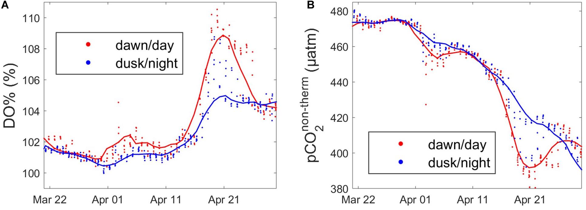
Figure 7. Diurnal variability of (A) DO% (%) and (B) pCO₂^non–therm (μatm) data extracted at dawn (red) and dusk (blue) ± 3 h during the productive period, from 22/03/2016 to 27/04/2016. Smooth lines in blue and red are obtained using a moving average filter with a 5-data span on the corresponding parameters.

Combining HF measurements of pH or pCO₂ with discrete carbonate system parameters (DIC/TA) can be a valuable tool for carbon cycle research based on autonomous mooring (Cullison Gray et al., 2011). Our robust TA/SSS relationship established in Section “Carbonate System Parameters” was concordant with similar relationships estimated in North Atlantic waters mixing with freshwater from non-limestone Irish rivers with similar TA end members (McGrath et al., 2016). We therefore estimated HF pH_calc for 2016, which varied from 8.00 during winter to 8.20 during summer (Figure 8A). These values were within the range of the in situ pH estimated between 7.97 and 8.35 by Marrec (2014) in the WEC and with pH values reported by McGrath et al. (2019) in Irish coastal waters (between 8.00 and 8.30). Unsurprisingly, pH_calc exhibited opposite dynamics to pCO₂ and was strongly related to the tidal signal. During spring/summer, low pH_calc values were observed at high tide and high pH_calc values at low tide, with 12-h variations up to 0.12 units (Figure 8B). The pH variability is particularly intense in coastal ecosystems (Ostle et al., 2016; Brodeur et al., 2019) resulting from various biogeochemical and physical processes (Waldbusser and Salisbury, 2014). In this study, most of the variability of pH_calc observed at the ASTAN site during spring likely resulted from tidal transport of the CWM and the OWM with contrasting biological and physical properties.

FIGURE 8

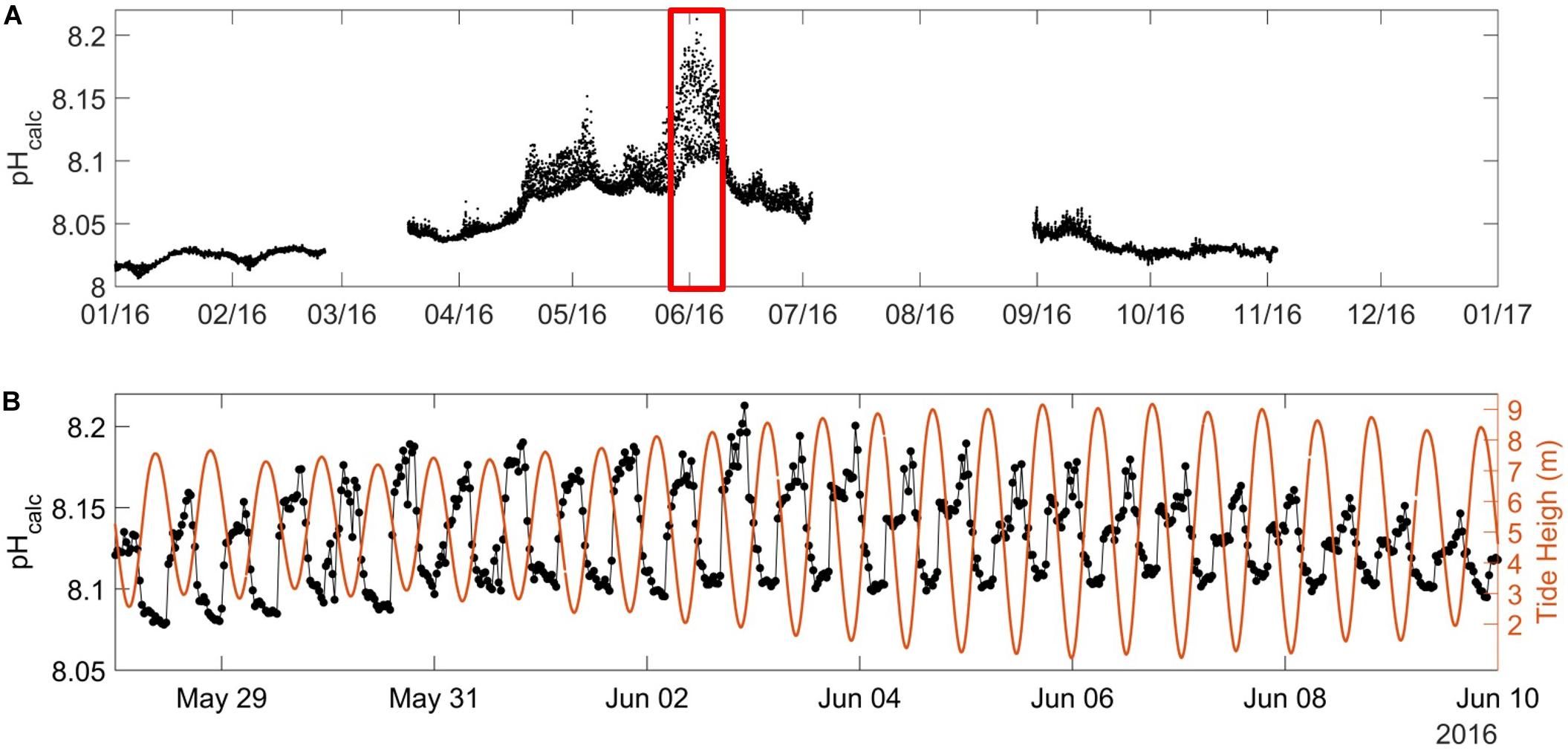
Figure 8. (A) pH_calc (in pH units on the total scale at in situ SST) at the ASTAN buoy during the year 2016 as explained in Section “Carbonate System Parameters” with (B) emphasis on the spring short-term variability of pH_calc (black dot) and the water level [in meters (orange line)] from 28/05/2016 to 09/06/2016.

Hydes et al. (2011) reported long-term pH decrease of −0.002 to −0.004 pH unit yr^–1 from 1995 to 2009 in the northwest European continental shelf, higher than in the Atlantic waters (Kitidis et al., 2017) and in the open ocean (Doney et al., 2009). At a daily time-scale, we observed variations up to 6 times greater than this regional annual acidification trend, and the seasonal variation was 10 times greater than the decadal change in the area. These strong variabilities are similar to the observations of McGrath et al. (2019) who reported, in similar coastal ecosystems in Ireland, a pH variability from 10 to 50 times greater than the decadal change linked to OA. Large changes of pCO₂ and pH were previously observed during short measurements period at fixed locations in various coastal ecosystems (Hofmann et al., 2011; Saderne et al., 2013). Intense changes in pH and saturation state Ω_arag have also been reported at coastal mooring sites in the California Current Ecoystem with natural variability overlapping with preindustrial conditions but also revealing critical OA conditions (Sutton et al., 2016). This variability has direct implications for calcifying species because variable pH exposure can affect organism response to OA (Vargas et al., 2017). Extremes decrease of Ω_arag have also been related to pteropods shell dissolution (Feely et al., 2016) and identified as a potential threat for the shellfish industry (Salisbury et al., 2008). Marine organisms in regions of persistent low pH might be locally adapted to OA (Sanford and Kelly, 2011; Pespeni et al., 2013). However, knowledge gaps about when and where corrosive conditions occur (Feely et al., 2016; Chan et al., 2017; Fennel et al., 2019) and how the timing of such conditions relates to key life stages (Legrand et al., 2017; Kapsenberg et al., 2018) still have to be filled to assess vulnerability to OA. Here we showed large daily changes in pH/pCO₂ but also DO/SST at the ASTAN mooring associated with the tidal transport of the CWM and the OWM in the nearshore area of the WEC over 5 years. These data can improve experimental design to evaluate organism response under real-world conditions by submitting these organisms to realistic variability in carbonate parameters (Chan et al., 2017) but also to varying DO and SST (Reum et al., 2016) instead of previous classical experimental designs (Noisette et al., 2016; Legrand et al., 2017) used in the WEC.

Seasonal and Interannual Control of pCO₂ in Coastal sWEC

Previous studies investigating the seasonal patterns of pCO₂ in the WEC indicated important physical and biological influence on carbonate cycling (Borges and Frankignoulle, 2003; Padin et al., 2007; Dumousseaud et al., 2010; Litt et al., 2010; Kitidis et al., 2012). With our 5 years of HF and discrete data we further investigated the seasonal and inter-annual variability of pCO₂ in the proximal area of the sWEC. Following the approach proposed by Takahashi et al. (1993, 2002), we discriminated the influence of thermal processes (pCO₂^therm) from non-thermal processes (pCO₂^non–therm) (Figures 9A,B) and we quantified the respective influence of δpCO₂^therm and δpCO₂^non–therm on pCO₂ (Figure 9C).

FIGURE 9

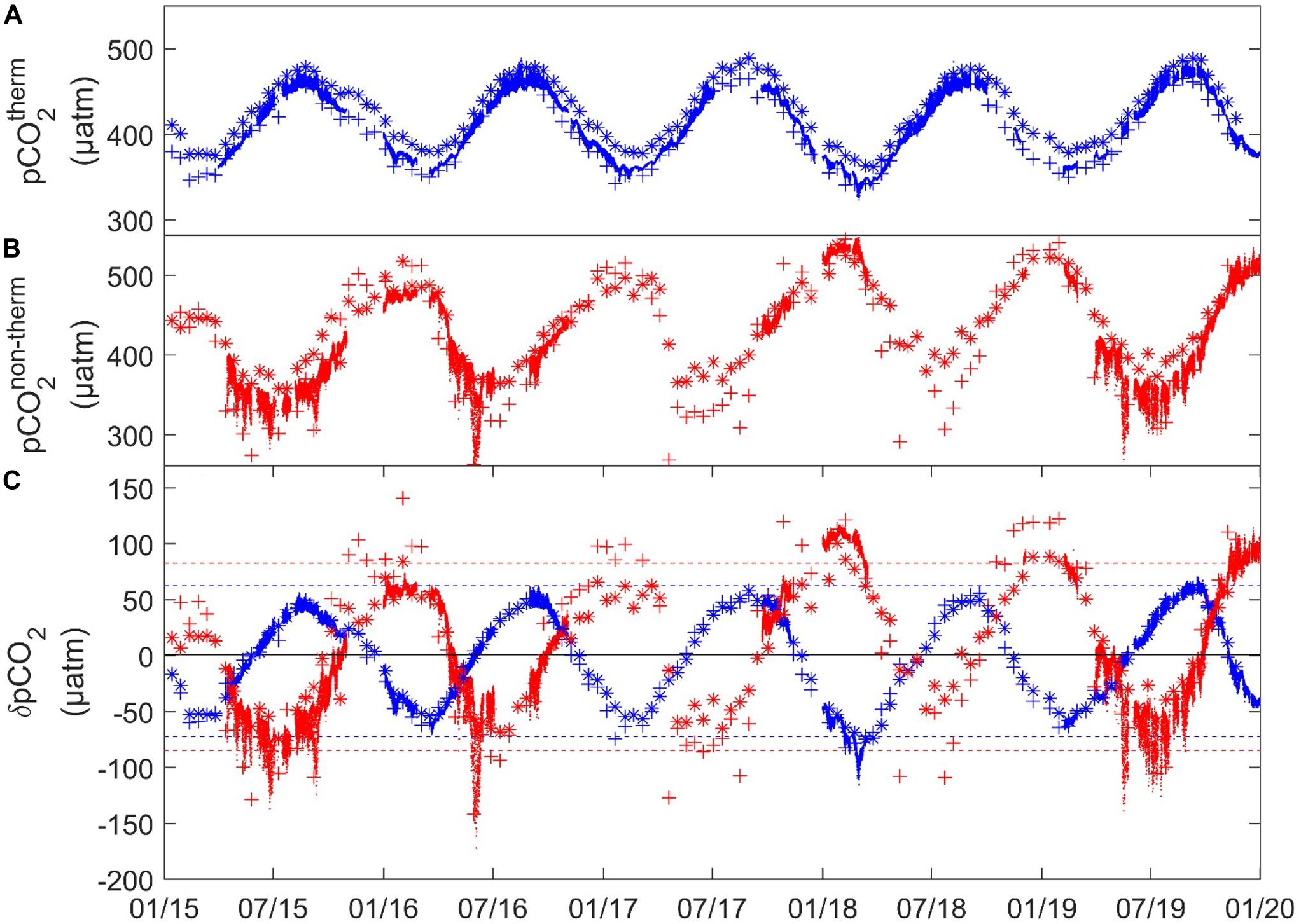
Figure 9. (A) pCO₂^therm (blue), (B) pCO₂^non–therm (red) (C) δpCO₂^therm = pCO₂-pCO₂^non–therm (blue) and δpCO₂^non–therm = pCO₂-pCO₂^therm (red) (all in μatm) for (.) High-frequency, (+) SOMLIT-pier, and (*) SOMLIT-offshore data. Dashed lines represent the maximum and minimum of the monthly mean of δpCO₂^therm (blue) and δpCO₂^non–therm (red).

The SST followed a rather regular pattern every year with limited inter-annual variations. Since pCO₂^therm is mainly influenced by temperature, we observed a variation of pCO₂^therm mirroring SST variations, varying from 325 to 490 μatm during winter and summer, respectively. δpCO₂^therm varied from + 67 μatm due to increasing SST during summer to −104 μatm due to decreasing SST during winter. In 2018, winter values diverged from the other years with lower SST (−1.5°C) compared to average values. Therefore, the lowest pCO₂^therm values (around 345 μatm) and a δpCO₂^therm of −104 μatm (20 μatm lower than the other years) were encountered that year. It is worth noting that during the same period SSS largely diverged from the average with values as low as 34.60, only recorded by HF monitoring. The decrease of pCO₂ induced by thermal processes was counterbalanced by particularly high pCO₂^non–therm values at this time (>500 μatm). The strong impact of non-thermal processes in winter 2018 might be related to intense riverine inputs, which brought a large amount of organic material. Besides this interannual variability, the 5-year dataset at the two discrete stations revealed spatial variability of the thermal effect on pCO₂. During winter, pCO₂^therm was lower at SOMLIT-pier (or CWM) compared to SOMLIT-offshore (or OWM), due to stronger cooling of nearshore waters during the winter regime. δpCO₂^therm revealed an impact 7 μatm higher of the SST cooling on pCO₂ in the CWM (Supplementary Table T1). During summer, after the shift from the winter to the summer regime, SST was higher at SOMLIT-pier than at SOMLIT-offshore. δpCO₂^therm showed that this higher SST was responsible for a potential increase of 5 μatm of pCO₂ in CWM compared to OWM (Supplementary Table T1).

Non-thermal effects on pCO₂, pCO₂^non–therm, are strongly influenced by biological production/respiration processes, but also by factors such as lateral advection, vertical mixing, air-sea CO₂ exchanges, dissolution/formation of CaCO₃, sediment/water-column interactions, or riverine inputs. However, this parameter remains a valuable and efficient approach to assess the impact of biological processes on pCO₂ variability (Thomas et al., 2005). Windspeed data (Supplementary Figure S4) showed a rather stable signal (higher values during winter’s storms and lower values during spring/summer) throughout the 5 years of study, which did not induce large inter-annual pCO₂^non–therm variability. The HF data showed a clear opposite dynamic between Chl-a-DO%, and the pCO₂^non–therm signals both temporally and in terms of intensity. The opposite patterns indicated that pCO₂^non–therm could reasonably be considered as an indicator to quantify the effect of biological processes on natural pCO₂ variability.

Spring in the sWEC is characterized by phytoplankton blooms between March and April fueled by the winter nutrient stock. The onset of spring phytoplankton blooms depends on light availability throughout the well-mixed water column (Wafar et al., 1983; L’Helguen et al., 1996). Surface waters, and the entire water column (except when weak and short stratification occurred), still exhibited relatively high Chl-a concentrations and oversaturated DO% along the summer since nutrient stocks (particularly nitrate) are rarely totally depleted because of the light limitation induced by strong mixing (Wafar et al., 1983; L’Helguen et al., 1996; Marrec, 2014). In fall, light availability becomes insufficient to support the substantial level of primary production required to maintain DO% oversaturation. Respiration and remineralization processes therefore become the main driver of pCO₂ variability, consuming DO, releasing CO₂, and driving the nutrient concentrations as in other temperate ecosystems of the northwest European continental shelf (Bozec et al., 2011; Marrec et al., 2013; Salt et al., 2016; Hartman et al., 2019). The biologically productive periods were accompanied by DO% > 100% and Chl-a concentrations > 1 μg L^–1 from April to October every year, with oxygen saturation reaching values up to 120%. During winter the heterotrophic activity (respiration and remineralization of organic matter) dominated with much lower Chl-a and undersaturated DO%. δpCO₂^non–therm showed a regular pattern driven by these production/respiration processes, with a strong coupling between the start/end of < 0 δpCO₂^non–therm and > 100% DO% values, and proved to be a suitable indicator of the extent and duration of the productive period (Figure 9C).

Important interannual variability was observed with respect to the onset and end of the productive period, as indicated by the DO% and δpCO₂^non–therm signals. In 2015, DO% started to be significantly higher than 100% in March, synchronized with an increase of Chl-a, and surface waters remained oversaturated in DO up to mid-September, while in 2018, the productive period started in May and ended in late August. 2018 was characterized by larger freshwater inputs (Figure 3B) due to heavy precipitations in late winter/early spring, and thus reduced light availability, associated with greater turbidity, which might have limited light penetration in the mixed water-column and thus delayed the start of the productive period. The pCO₂^non–therm and δpCO₂^non–therm signals followed similar dynamics. In 2015, pCO₂^non–therm and δpCO₂^non–therm started to decrease and to be negative, respectively, in April, whereas negative δpCO₂^non–therm started to be observed in May in 2018. Positive δpCO₂^non–therm values were observed from September in 2015 and from August in 2018. The decrease of pCO₂^non–therm in spring can be particularly rapid, as in spring 2016 with a drawdown of around 250 μatm during a 2-month period (March–May), revealing a large consumption of pCO₂ by biological activity partly counteracted by the increasing SST and pCO₂^therm at the same period.

Spatial variability was visible from the discrete data, particularly in summer, when pCO₂^non–therm was persistently lower at SOMLIT-pier (CWM) than at SOMLIT-offshore (OWM). During the productive period, seasonal minimal δpCO₂^non–therm values lower than −100 μatm were observed in the CWM every year, while the δpCO₂^non–therm signals never reached values below −70 μatm in the OWM. The shallower depth in the CMW favors light penetration, which can result in higher pelagic production (when nutrients are not depleted) compared to the deeper OWM. The role of benthic production processes on CO₂ variations is also important in proximal shallow areas (Hammond et al., 1999; Cai et al., 2000; Forja et al., 2004; Waldbusser and Salisbury, 2014; Oliveira et al., 2018). The low δpCO₂^non–therm associated to CWM during the productive period might include both higher pelagic and benthic production, with a predominance of the latter. The tidal transport of the CWM over adjacent seagrass and macroalgae beds with high CO₂ consumption (Ouisse et al., 2011; Bordeyne et al., 2017) extended the biological productive period of the CWM to the benthic compartment. The δpCO₂^non–therm seasonal mean difference of 30 μatm recorded between both stations was therefore a gross estimation of the benthic compartment production within the nearshore area. Similarly, a nearshore to offshore gradient was observed during fall and early winter. Values of δpCO₂^non–therm in the CWM of 130 μatm were 40 μatm higher than in the OWM, the important benthic and pelagic remineralization in the shallower CWM contributing to a larger increase of pCO₂. This increase was partly counteracted by the decreasing pCO₂^therm due to fall and winter SST cooling as discussed above.

Our data revealed a somewhat classical picture of pCO₂ control in temperate ecosystems with counteracting effects of thermodynamic and biological activity depending on the seasons (Thomas et al., 2005; Bozec et al., 2011). The combined 5-year HF and discrete data allowed for the first time the quantification of rather large interannual and spatial variability in the proximal surface waters of the sWEC. Non-thermal processes, that we assumed to be mainly controlled by biological activity, were the main driver of pCO₂ in the coastal sWEC, as shown by the larger amplitude, both during winter and summer, of pCO₂^non–therm compared to pCO₂^therm. The interannual variability of pCO₂ depended mainly on the duration and the intensity of the productive period. The weak interannual variability in terms of SST limited its control over the 5 years of study on pCO₂ compared to production/respiration processes.

Dynamics of FCO₂ in the WEC

Our study provides FCO₂ estimates at daily, seasonal and annual time scales. One major limitation for estimating HF FCO₂ is the requirement to access HF atmospheric CO₂ data in the surrounding study area. Northcott et al. (2019) recently demonstrated the impact of higher atmospheric CO₂ transported by offshore winds from urban and agricultural land on FCO₂ estimates in Monterey Bay, California. This concern was also addressed by Wimart-Rousseau et al. (2020) in their study of FCO₂ in the vicinity of a highly urbanized area. Unfortunately, we did not have access to local HF atmospheric CO₂ data, so atmospheric xCO₂ data from the RAMCES network collected at the Mace Head site (53°33′ N 9°00′ W, southern Ireland) were used to calculate pCO₂^atm. The dominant onshore south-westerly winds and rather lowly urbanized surroundings in our study area mean that the Mace Head record should be representative of our study site. The use of local wind products from the nearby Guipavas weather station (Supplementary Figure S4) and of recent gas transfer velocity parametrization adapted to regional estimates (Wanninkhof, 2014) limited the error linked to different wind products in regional air-sea flux estimations (Roobaert et al., 2018). The impact of rain, extreme wind events and associated bubble entrainment, surface films or boundary layer stability (Wanninkhof et al., 2009 for a review) are factors inducing additional uncertainty into gas transfer velocity k, and therefore HF FCO₂ calculation, but remain particularly difficult to assess. The eddy covariance technique, as used by Yang et al. (2019) in the nWEC, can overcome most of these limitations inherent to gas transfer velocity parametrization, and presents some undeniable advantages for studying HF FCO₂. However, the use of in situ seawater pCO₂ sensor remained the most effective way to study pCO₂, examine its control, and simultaneously estimate air-sea CO₂ fluxes using widely used wind dependent gas transfer velocity parametrization.

The main benefit of HF data was to assess daily FCO₂ variability and capture extreme events such as high fluxes observed during winter or abrupt shifts and drawdown during spring. For example, during winter 2017 a HF FCO₂ of 26 mmol C m^–2 d^–1 was recorded at ASTAN compared to values of 3 mmol C m^–2 d^–1 computed from discrete values at the same time. During spring, as explained in Section “Seasonal and Interannual Control of pCO₂ in Coastal WEC,” the large interannual variability of the intensity and trigger of spring blooms was responsible for variable spring drawdown in pCO₂, revealing sudden and strong inversions of the fluxes. For example, in March 2016 FCO₂ was on average positive with a monthly maximum of + 5.93 mmol C m^–2 d^–1 (03/27/16), and within a few days became negative, with a monthly minimum of −4.42 mmol C m^–2 d^–1 (04/19/16). This large daily variability should be taken into account when considering the spring average carbon sink for each year (with a mean estimate at −2.12 mmol C m^–2 d^–1). With the method applied in Section “Short-Scale Variability of the CO₂ System in Coastal sWEC” we were able to separate the day/night signal during this period and found a mean difference of FCO₂ of −0.12 mmol m^–2 d^–1 due to the diel biological cycle. This estimation was understandably lower than the day–night difference estimated at −0.90 mmol m^–2 d^–1 for FCO₂ during spring in the stratified and more productive nWEC (Marrec et al., 2014). FCO₂ based on HF data provided relevant information on short-term variability, the main caveat of the cardinal buoy data being the significant loss of data, which hindered computation of mean seasonal averages.

The mean seasonal FCO₂ values for the three sites during the 5 years of study were compared to assess the seasonal and spatial variability of FCO₂ along a coastal/offshore gradient (Figure 4). FCO₂ computed from the HF data at ASTAN exhibited similar overall variability as FCO₂ obtained from discrete measurements at SOMLIT-pier (CWM) and at SOMLIT-offshore (OWM). Similar general patterns between HF and discrete data at the seasonal level have also been reported in recent studies (Shadwick et al., 2019). Regardless of sampling frequency and locations, the three studied sites acted as strong sources of CO₂ to the atmosphere during winter/fall. During spring, SOMLIT-pier and ASTAN acted as sinks of atmospheric CO₂, with higher CO₂ sink at SOMLIT-pier than at ASTAN, while fluxes computed at SOMLIT-offshore indicated exchanges near equilibrium. Summer was the only time of the year when significant differences in terms of flux intensity and direction were observed between the three sites. This time of the year corresponds to the shift from dominant production of organic matter by photosynthetic organisms toward dominant remineralization and respiration processes, which usually start earlier in the deeper well-mixed water column at SOMLIT-offshore. The 2015/2018 years were marked by large differences in terms of the date of onset and length of the productive period, which were poorly reflected in the mean seasonal spring and summer FCO₂. However, the following fall was marked by large differences in terms of emissions of CO₂ to the atmosphere, much lower in 2018 compared to 2015 when it was driven by high wind speeds (maximum monthly mean of 9.7 m s^–1). The mean wind speeds recorded during fall 2018 (4.6 m s^–1) were followed by lower than average wind speeds the following winter months (4.6 m s^–1 compared to mean 5.2 m s^–1) (Figure 3), which still resulted in significant flux differences, driven this time by the delayed remineralization period (Figure 4). This study confirms that seasonal variability of FCO₂ in this part of the NE European continental shelf is controlled by complex interactions between high/low wind speeds, production/respiration of organic matter and winter cooling (Kitidis et al., 2019).

On an annual basis, given the dominant impact of the tidal cycle at ASTAN, it seemed particularly interesting to assess the proximal coastal/offshore gradient of FCO₂ from the buoy data only. In 2016/2019 the HF dataset was sufficiently complete to attempt an estimation of annual FCO₂ in the CMW and OMW based on tidal separation of the HF signal. We separated the dataset according to high tides (>8 m) and low tides (<2.5 m), as previously explained. The annual mean FCO₂ over 2016/2019 was estimated at 0.37 mol C m^–2 yr^–1 for the CMW and 0.65 mol C m^–2 yr^–1 for the OWM (Figure 10). The mean HF FCO₂ of 0.51 mol C m^–2 yr^–1 for 2016/2019 at the ASTAN buoy was obviously within the range of FCO₂ in the CWM and OWM. FCO₂ computed at ASTAN comprised both the tidal and diurnal signals and was therefore representative of nearshore surface waters in the sWEC. Comparison of these HF budget with the annual mean budget for 2016/2019 based on discrete sampling at SOMLIT-pier (0.35 mol C m^–2 yr^–1) and SOMLIT-offshore (0.62 mol C m^–2 yr^–1), which we assumed representative of the CWM and OWM, respectively, revealed very similar values. Here, the arbitrary separation of the HF data according to tide levels provided coherent results with discrete samples collected at noon during neap tides at both SOMLIT stations. We were able to estimate FCO₂ in the CWM and OWM with the ASTAN mooring, which underly the great potential of cardinal buoys to capture the dynamic of FCO₂ in nearshore tidal ecosystems. It is worth noting that CO₂ emissions at SOMLIT-offshore (averaged over the 5-year period) showed a similar trend but lower values than emissions computed from 2011 to 2013 at the same site (Figure 10), with an atmospheric CO₂ increase of + 9 to + 15 μatm recorded between the studies. These new estimates in nearshore waters of the sWEC over a 5-year period combined with previous studies provided a full latitudinal representation over multiple years for FCO₂ in the WEC (Figures 1, 10). This is particularly relevant since proximal areas are currently excluded from global estimates in the coastal ocean (Bourgeois et al., 2016). The latitudinal comparison showed a clear gradient from a weak source of CO₂ in the tidal mixing areas toward sinks of CO₂ in the stratified regions less influenced by tidal mixing in agreement with recent global modeling studies (Laruelle et al., 2018). Interestingly, in the tidal mixing ecosystems the sources increased from nearshore to offshore waters, whereas in stratified ecosystems the sink increased toward nearshore waters. Andersson and Mackenzie (2004) first suggested that shelves may have turned from a CO₂ source in the preindustrial time to a sink at present and that the CO₂ uptake rate would increase with time. More recently Cai (2011) and Bauer et al. (2013) suggested an increasing global shelf CO₂ sink with time as a result of the atmospheric pCO₂ increase. The latest SOCAT data confirm this trend with a slower pCO₂ increase in shelf waters compared to atmospheric pCO₂ that could increase the air-sea gradient and thus the uptake of atmospheric CO₂ in the decades to come, although high spatial variability in air–sea fluxes is to be expected across shelf regions (Laruelle et al., 2018). This is particularly significant for the sWEC, which is a weak source of CO₂ and could potentially become a sink of CO₂ in the coming decades.

FIGURE 10

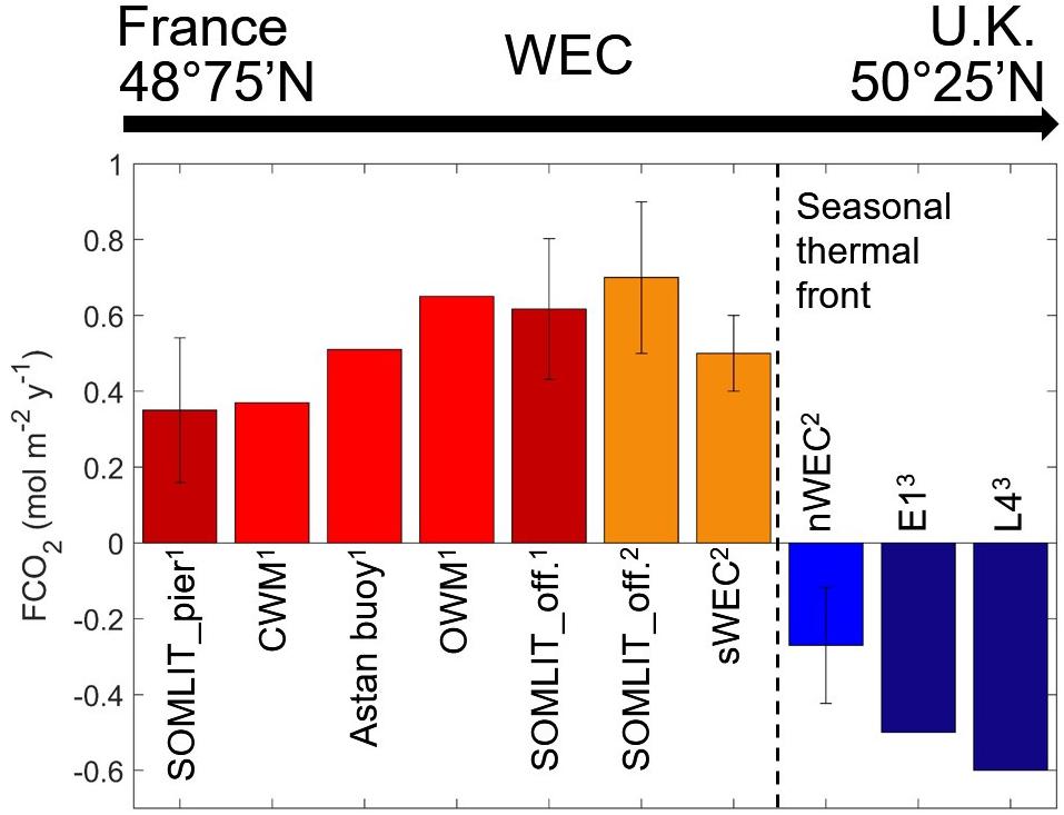
Figure 10. Annual mean FCO₂ (mol C m^–2 y^–1) across the WEC at discrete stations SOMLIT-pier and SOMLIT-offshore for the 2015–2019 period (dark red), in the CMW, OMW and at ASTAN based on HF data from 2016 and 2019 (red) from this study¹; at SOMLIT-offshore (orange), in the sWEC (orange) and nWEC (blue) for the period 2011–2013 from Marrec (2014)²; and at discrete stations E1 and L4 (dark blue) for the period 2007–2010 from Kitidis et al. (2012)³.

Conclusion

The recent OceanObs 2019 conference highlighted the need for innovative and sustained coastal observatories (Farcy et al., 2019) notably for the study of FCO₂. In the last decade, the emergence of new high-performance pH and pCO₂ sensors has been extremely valuable for the investigation of OA and FCO₂ (Sastri et al., 2019). Here, the implementation of a cardinal buoy of opportunity equipped with such novel sensors into an existing network of time-series and Ferrybox monitoring programs provided a robust multiple year assessment of FCO₂ and also pH variability in a temperate coastal ecosystem. This is particularly relevant on a socio-economical level since nearshore ecosystems host large stocks of shellfish species sensitive to ongoing ocean acidification. Numerous cardinal buoys are present in the global coastal ocean to direct traffic, particularly along rocky shores with large tidal ranges. These buoys of opportunity can be equipped with meteorological and oceanographic sensors and transmit data daily to the shore, thus providing real-time data for the study of coastal ecosystems under climate change. This network of buoys therefore has significant potential to be exploited for efficient, low cost observation of coastal ecosystems.

Data Availability Statement

Discrete data are available at: http://somlit-db.epoc.u-bordeaux1.fr/bdd.php?serie=ST&sm=3 (accessed date 14 August 2020).

Author Contributions

J-PG collected, analyzed, processed and interpreted the data, and wrote the first version of the manuscript. PM provided scientific discussion, new ideas on the interpretation of the results, and contributed to writing the manuscript. TC initiated the collaboration on the Cardinal buoy. TC, CG, ÉM, and MV configured the data acquisition system on the buoy, calibrated and cleaned the sensors, collected data in the field, analyzed discrete samples in the laboratory and processed the data. YB designed the study, led the research, interpreted the data, wrote the manuscript, and managed the project. All authors contributed to the article and approved the submitted version.

Funding

This work was funded by the CNRS through INSU [COAST HF, SOMLIT, project CHANNEL (LEFE/CYBER)] and INEE, by the “Conseil Général du Finistère” (CD29) and by the “Region Bretagne” (program ARED, project Hi-Tech). Part of this work was supported by the JERICO-NEXT project from the European Union’s Horizon 2020 Research and Innovation Program under grant agreement no. 654410. YB is P.I. of the CHANNEL and Hi-Tech projects and associate researcher (CRCN) at CNRS. J-PG holds a Ph.D. grant from the Region Bretagne and Sorbonne University (ED129).

Conflict of Interest

The authors declare that the research was conducted in the absence of any commercial or financial relationships that could be construed as a potential conflict of interest.

Acknowledgments

We thank the “Service des Phares et Balises” for providing access to the ASTAN buoy and the “Service Mer” of the SBR for their valuable support during sampling at sea. We thank the SNAPOCO2 for DIC/TA analysis and M. Ramonet for providing the atmospheric CO₂ data from the RAMCES network (Observatory Network for Greenhouse gases). G. Charia (Ifremer) provided valuable help with the wavelet frequency analysis. We thank the SOMLIT (Service d’Obervation du Milieu LIToral) network for providing oceanographic data at the SOMLIT sites and help during fieldwork. We thank A. Durand and E. Collin for their help during field campaign on the Penzé river. We are grateful to the Menden-Deuer lab (URI-GSO) and A. C. Baudoux for constructive collaboration and scientific discussions during finalization of the manuscript. We thank I. Probert for correcting the revised manuscript and the two reviewers whose comments greatly improved the quality of the manuscript. In memory of FB.

Supplementary Material

The Supplementary Material for this article can be found online at: https://www.frontiersin.org/articles/10.3389/fmars.2020.00712/full#supplementary-material

Footnotes

1. ^ http://somlit.epoc.u-bordeaux1.fr/
2. ^ http://coast-hf.fr

References

Alpine, A. E., and Cloern, J. E. (1985). Differences in in vivo fluorescence yield between three phytoplankton size classes. J. Plankton Res. 7, 381–390. doi: 10.1093/plankt/7.3.381

PubMed Abstract | CrossRef Full Text | Google Scholar

Aminot, A., and Kérouel, R. (2007). Dosage Automatique des Nutriments dans les Eaux Marines: Méthodes en Flux Continu. Brest: Ifremer.

Google Scholar

Andersson, A. J., and Mackenzie, F. T. (2004). Shallow-water oceans: a source or sink of atmospheric CO2? Front. Ecol. Environ. 2:348–353.

Google Scholar

Bakker, D. C., Pfeil, B., Landa, C. S., Metzl, N., O’Brien, K. M., Olsen, A., et al. (2016). A multi-decade record of high-quality fCO2 data in version 3 of the Surface Ocean CO2 Atlas (SOCAT). Earth Syst. Sci. Data 8, 383–413.

Google Scholar

Bauer, J. E., Cai, W. J., Raymond, P. A., Bianchi, T. S., Hopkinson, C. S., and Regnier, P. A. (2013). The changing carbon cycle of the coastal ocean. Nature 504, 61–70. doi: 10.1038/nature12857

PubMed Abstract | CrossRef Full Text | Google Scholar

Beucher, C., Treguer, P., Corvaisier, R., Hapette, A. M., and Elskens, M. (2004). Production and dissolution of biosilica, and changing microphytoplankton dominance in the Bay of Brest (France). Mar. Ecol. Prog. Ser. 267, 57–69. doi: 10.3354/meps267057

CrossRef Full Text | Google Scholar

Bordeyne, F., Migné, A., and Davoult, D. (2017). Variation of fucoid community metabolism during the tidal cycle: insights from in situ measurements of seasonal carbon fluxes during emersion and immersion. Limnol. Oceanogr. 62, 2418–2430. doi: 10.1002/lno.10574

CrossRef Full Text | Google Scholar

Borges, A. V., Alin, S. R., Chavez, F. P., Vlahos, P., Johnson, K. S., Holt, J. T., et al. (2010). “A global sea surface carbon observing system: inorganic and organic carbon dynamics in coastal oceans,” in Proceedings of OceanObs’09: Sustained Ocean Observations and Information for Society, Vol. 2, (Paris: European Space Agency), 67–88. doi: 10.5270/OceanObs09.cwp.07

CrossRef Full Text | Google Scholar

Borges, A. V., and Frankignoulle, M. (2003). Distribution of surface carbon dioxide and air sea exchange in the English Channel and adjacent areas. J. Geophys. Res. Oceans 108:3140. doi: 10.1029/2000JC000571

CrossRef Full Text | Google Scholar

Borges, A. V., and Gypens, N. (2010). Carbonate chemistry in the coastal zone responds more strongly to eutrophication than ocean acidification. Limnol. Oceanogr. 55, 346–353.

Google Scholar

Bourgeois, T., Orr, J. C., Resplandy, L., Terhaar, J., Ethé, C., Gehlen, M., et al. (2016). Coastal-ocean uptake of anthropogenic carbon. Biogeosciences 13, 4167–4185. doi: 10.5194/bg-13-4167-2016

CrossRef Full Text | Google Scholar

Bozec, Y., Cariou, T., Macé, E., Morin, P., Thuillier, D., and Vernet, M. (2012). Seasonal dynamics of air-sea CO2 fluxes in the inner and outer Loire estuary (NW Europe). Estuar. Coast. Shelf Sci. 100, 58–71.

Google Scholar

Bozec, Y., Merlivat, L., Baudoux, A. C., Beaumont, L., Blain, S., Bucciarelli, E., et al. (2011). Diurnal to inter-annual dynamics of pCO2 recorded by a CARIOCA sensor in a temperate coastal ecosystem (2003–2009). Mar. Chem. 126, 13–26. doi: 10.1016/j.marchem.2011.03.003

CrossRef Full Text | Google Scholar

Bricaud, A., Babin, M., Morel, A., and Claustre, H. (1995). Variability in the chlorophyll-specific absorption coefficients of natural phytoplankton: analysis and parameterization. J. Geophys. Res. Oceans 100, 13321–13332. doi: 10.1029/95JC00463

CrossRef Full Text | Google Scholar

Bricaud, A., Morel, A., and Prieur, L. (1983). Optical efficiency factors of some phytoplankters 1. Limnol. Oceanogr. 28, 816–832. doi: 10.4319/lo.1983.28.5.0816

CrossRef Full Text | Google Scholar

Brodeur, J. R., Chen, B., Su, J., Xu, Y. Y., Hussain, N., Scaboo, K. M., et al. (2019). Chesapeake Bay inorganic carbon: spatial distribution and seasonal variability. Front. Mar. Sci. 6:99. doi: 10.3389/fmars.2019.00099

CrossRef Full Text | Google Scholar

Cai, W.-J. (2011). Estuarine and coastal ocean carbon paradox: CO2 sinks or sites of terrestrial carbon incineration? Annu. Rev. Mar. Sci. 3, 123–145.

Google Scholar

Cai, W. J., Hu, X., Huang, W. J., Murrell, M. C., Lehrter, J. C., Lohrenz, S. E., et al. (2011). Acidification of subsurface coastal waters enhanced by eutrophication. Nat. Geosci. 4, 766–770. doi: 10.1038/ngeo1297

CrossRef Full Text | Google Scholar

Cai, W.-J., Huang, W.-J., Luther, G. W., Pierrot, D., Li, M., Testa, J., et al. (2017). Redox reactions and weak buffering capacity lead to acidification in the Chesapeake Bay. Nat. Commun. 8:369. doi: 10.1038/s-017-00417-7

CrossRef Full Text | Google Scholar

Cai, W. J., Wiebe, W. J., Wang, Y., and Sheldon, J. E. (2000). Intertidal marsh as a source of dissolved inorganic carbon and a sink of nitrate in the Satilla River-estuarine complex in the southeastern US. Limnol. Oceanogr. 45, 1743–1752. doi: 10.4319/lo.2000.45.8.1743

CrossRef Full Text | Google Scholar

Carberry, L., Roesler, C., and et Drapeau, S. (2019). Correcting in situ chlorophyll fluorescence time-series observations for nonphotochemical quenching and tidal variability reveals nonconservative phytoplankton variability in coastal waters. Limnol. Oceanogr. Methods 17, 462–473. doi: 10.1002/lom3.10325

PubMed Abstract | CrossRef Full Text | Google Scholar

Carpenter, J. H. (1965). The accuracy of the winkler method for dissolved oxygen analyisis. Limnol. Oceanogr. 10, 135–140.

Google Scholar

Cazelles, B., Chavez, M., Berteaux, D., Ménard, F., Vik, J. O., Jenouvrier, S., et al. (2008). Wavelet analysis of ecological time series. Oecologia 156, 287–304. doi: 10.1007/s00442-008-0993-2

PubMed Abstract | CrossRef Full Text | Google Scholar

Chan, F., Barth, J. A., Blanchette, C. A., Byrne, R. H., Chavez, F., Cheriton, O., et al. (2017). Persistent spatial structuring of coastal ocean acidification in the California Current System. Sci. Rep. 7:2526. doi: 10.1038/s41598-017-02777-y

PubMed Abstract | CrossRef Full Text | Google Scholar

Chen, C. T. A., and Borges, A. V. (2009). Reconciling opposing views on carbon cycling in the coastal ocean: continental shelves as sinks and near-shore ecosystems as sources of atmospheric CO2. Deep Sea Res. Part II Top. Stud. Oceanogr. 56, 578–590.

Google Scholar

Chierici, M., Fransson, A., and Anderson, L. G. (1999). Influence of m-cresol purple indicator additions on the pH of seawater samples: correction factors evaluated from a chemical speciation model. Mar. Chem. 65, 281–290. doi: 10.1016/S0304-4203(99)00020-1

CrossRef Full Text | Google Scholar

Ciais, P., Sabine, C., Bala, G., Bopp, L., Brovkin, V., Canadell, J., et al. (2014). “Carbon and other biogeochemical cycles,” in Climate change 2013: the physical Science Basis. Contribution of Working Group I to the Fifth Assessment Report of the Intergovernmental Panel on Climate Change, eds T. F. Stocker, D. Qin, G.-K. Plattner, M. Tignor, S. K. Allen, et al. (Cambridge: Cambridge University Press), 465–570.

Google Scholar

Clayton, T. D., and Byrne, R. H. (1993). Spectrophotometric seawater pH measurements: total hydrogen ion concentration scale calibration of m-cresol purple and at-sea results. Deep Sea Res. Part I Oceanogr. Res. Pap. 40, 2115–2129. doi: 10.1016/0967-0637(93)90048-8

CrossRef Full Text | Google Scholar

Cullison Gray, S. E., DeGrandpre, M. D., Moore, T. S., Martz, T. R., Friederich, G. E., and Johnson, K. S. (2011). Applications of in situ pH measurements for inorganic carbon calculations. Mar. Chem. 125, 82–90. doi: 10.1016/j.marchem.2011.02.005

CrossRef Full Text | Google Scholar

Dai, M., Lu, Z., Zhai, W., Chen, B., Cao, Z., Zhou, K., et al. (2009). Diurnal variations of surface seawater pCO2 in contrasting coastal environments. Limnol. Oceanogr. 54, 735–745. doi: 10.4319/lo.2009.54.3.0735

CrossRef Full Text | Google Scholar

DeGrandpre, M. D., Hammar, T. R., Wallace, D. W., and Wirick, C. D. (1997). Simultaneous mooring-based measurements of seawater CO2 and O2 off Cape Hatteras, North Carolina. Limnol. Oceanogr. 42, 21–28. doi: 10.4319/lo.1997.42.1.0021

CrossRef Full Text | Google Scholar

DeGrandpre, M. D., Hammar, T. R., and Wirick, C. D. (1998). Short-term pCO₂ and O₂ dynamics in California coastal waters. Deep Sea Res. Part II: Top. Stud. Oceanogr. 45, 1557–1575. doi: 10.1016/S0967-0645(98)80006-4

CrossRef Full Text | Google Scholar

de Haas, H., van Weering, T. C., and de Stigter, H. (2002). Organic carbon in shelf seas: sinks or sources, processes and products. Cont. Shelf Res. 22, 691–717. doi: 10.1016/S0278-4343(01)00093-0

CrossRef Full Text | Google Scholar

De la Paz, M., Gómez-Parra, A., and Forja, J. (2007). Inorganic carbon dynamic and air–water CO2 exchange in the Guadalquivir Estuary (SW Iberian Peninsula). J. Mar. Syst. 68, 265–277. doi: 10.1016/j.jmarsys.2006.11.011

CrossRef Full Text | Google Scholar

Del Amo, Y., Quéguiner, B., Tréguer, P., Breton, H., and Lampert, L. (1997). Impacts of high-nitrate freshwater inputs on macrotidal ecosystems. II. Specific role of the silicic acid pump in the year-round dominance of diatoms in the Bay of Brest (France). Mar. Ecol. Prog. Ser. 161, 225–237. doi: 10.3354/meps161225

CrossRef Full Text | Google Scholar

Dickson, A. G., and Millero, F. J. (1987). A comparison of the equilibrium constants for the dissociation of carbonic acid in seawater media. Deep Sea Res. Part A Oceanogr. Res. Pap. 34, 1733–1743. doi: 10.1016/0198-0149(87)90021-5

CrossRef Full Text | Google Scholar

Dickson, A. G., Sabine, C. L., and Christian, J. R. (eds) (2007). Guide to Best Practices for Ocean CO2 Measurements. North Pacific Marine Science Organization, 176. Available online at: www.nodc.noaa.gov/ocads/oceans/Handbook_2007.html (accessed July 17, 2020).

Google Scholar

DOE (1994). Handbook of Methods for Analysis of the Various Parameters of the Carbon Dioxide System in Sea Water, Version 2. Available online at: https://core.ac.uk/download/pdf/98639593.pdf doi: 10.2172/10107773 (accessed July 17, 2020).

CrossRef Full Text | PubMed Abstract | Google Scholar

Doney, S. C., Fabry, V. J., Feely, R. A., and Kleypas, J. A. (2009). Ocean acidification: the other CO2 problem. Annu. Rev. Mar. Sci. 1, 169–192. doi: 10.1146/annurev.marine.010908.163834

PubMed Abstract | CrossRef Full Text | Google Scholar

Dumousseaud, C., Achterberg, E. P., Tyrrell, T., Charalampopoulou, A., Schuster, U., Hartman, M., et al. (2010). Contrasting effects of temperature and winter mixing on the seasonal and inter-annual variability of the carbonate system in the Northeast Atlantic, Ocean. Biogeosciences 7, 1481–1492. doi: 10.5194/bg-7-1481-2010

CrossRef Full Text | Google Scholar

Dürr, H. H., Meybeck, M., Hartmann, J., Laruelle, G. G., and Roubeix, V. (2011). Global spatial distribution of natural riverine silica inputs to the coastal zone. Biogeosciences 8, 597–620. doi: 10.5194/bg-8-597-2011

CrossRef Full Text | Google Scholar

Edmond, J. M. (1970). High precision determination of titration alkalinity and total carbon dioxide content of sea water by potentiometric titration. Deep Sea Res. Oceanogr. Abstr. 17, 737–750. doi: 10.1016/0011-7471(70)90038-0

CrossRef Full Text | Google Scholar

Farcy, P., Durand, D., Charria, G., Painting, S. J., Collingridge, K., Grémare, A. J., et al. (2019). Towards a European Coastal Observing Network to provide better answer to science and to societal challenges; the JERICO/JERICO-NEXT Research Infrastructure. Front. Mar. Sci. 6:529. doi: 10.3389/fmars.2019.00529

CrossRef Full Text | Google Scholar

Feely, R. A., Alin, S., Carter, B., Bednaršek, N., Hales, B., Chan, F., et al. (2016). Chemical and biological impacts of ocean acidification along the west coast of North America. Estuar. Coast. Shelf Sci. 183, 260–270. doi: 10.1016/j.ecss.2016.08.043

CrossRef Full Text | Google Scholar

Feely, R. A., Alin, S. R., Newton, J., Sabine, C. L., Warner, M., Devol, A., et al. (2010). The combined effects of ocean acidification, mixing, and respiration on pH and carbonate saturation in an urbanized estuary. Estuar. Coast. Shelf Sci. 88, 442–449. doi: 10.1016/j.ecss.2010.05.004

CrossRef Full Text | Google Scholar

Fennel, K., Alin, S., Barbero, L., Evans, W., Bourgeois, T., Cooley, S., et al. (2019). Carbon cycling in the North American coastal ocean: a synthesis. Biogeosciences 16, 1281–1304.

Google Scholar

Forja, J. M., Ortega, T., DelValls, T. A., and Gómez-Parra, A. (2004). Benthic fluxes of inorganic carbon in shallow coastal ecosystems of the Iberian Peninsula. Mar. Chem. 85, 141–156. doi: 10.1016/j.marchem.2003.09.007

CrossRef Full Text | Google Scholar

Friedlingstein, P., Jones, M., O’sullivan, M., Andrew, R., Hauck, J., Peters, G. et al. (2019). Global carbon budget 2019. Earth Syst. Sci. Data 11, 1783–1838. doi: 10.5194/essd-11-1783-2019

CrossRef Full Text | Google Scholar

Gattuso, J. P., Frankignoulle, M., and Wollast, R. (1998). Carbon and carbonate metabolism in coastal aquatic ecosystems. Annu. Rev. Ecol. Syst. 29, 405–434. doi: 10.1146/annurev.ecolsys.29.1.405

CrossRef Full Text | Google Scholar

Goring, D. G., and Bell, R. G. (1999). El Niño and decadal effects on sea-level variability in northern New Zealand: a wavelet analysis. N. Z. J. Mar. Freshw. Res. 33, 587–598. doi: 10.1080/00288330.1999.9516902

CrossRef Full Text | Google Scholar

Gran, G. (1952). Determination of the equivalence point in potentiometric titrations. Part II. Analyst 77, 661–671.

Google Scholar

Grinsted, A., Moore, J. C., and Jevrejeva, S. (2004). Application of the cross wavelet transform and wavelet coherence to geophysical time series. Nonlinear Process. Geophys. 11, 561–566.

Google Scholar

Gruber, N., Clement, D., Carter, B. R., Feely, R. A., Van Heuven, S., Hoppema, M., et al. (2019). The oceanic sink for anthropogenic CO2 from 1994 to 2007. Science 363, 1193–1199. doi: 10.1126/science.aau5153

PubMed Abstract | CrossRef Full Text | Google Scholar

Guilloux, L., Rigaut-Jalabert, F., Jouenne, F., Ristori, S., Viprey, M., Not, F., et al. (2013). An annotated checklist of Marine Phytoplankton taxa at the SOMLIT-Astan time series off Roscoff (Western English Channel, France): data collected from 2000 to 2010. Cah. Biol. Mar. 54, 247–256.

Google Scholar

Hammond, D. E., Giordani, P., Berelson, W. M., and Poletti, R. (1999). Diagenesis of carbon and nutrients and benthic exchange in sediments of the Northern Adriatic Sea. Mar. Chem. 66, 53–79. doi: 10.1016/S0304-4203(99)00024-9

CrossRef Full Text | Google Scholar

Haraldsson, C., Anderson, L. G., Hassellöv, M., Hulth, S., and Olsson, K. (1997). Rapid, high-precision potentiometric titration of alkalinity in ocean and sediment pore waters. Deep Sea Res. Part I Oceanogr. Res. Pap. 44, 2031–2044. doi: 10.1016/S0967-0637(97)00088-5

CrossRef Full Text | Google Scholar

Hartman, S. E., Humphreys, M. P., Kivimäe, C., Woodward, E. M. S., Kitidis, V., McGrath, T., et al. (2019). Seasonality and spatial heterogeneity of the surface ocean carbonate system in the northwest European continental shelf. Prog. Oceanogr. 177:101909. doi: 10.1016/j.pocean.2018.02.005

CrossRef Full Text | Google Scholar

Hofmann, G. E., Smith, J. E., Johnson, K. S., Send, U., Levin, L. A., Micheli, F., et al. (2011). High-frequency dynamics of ocean pH: a multi-ecosystem comparison. PLoS One 6:e28983. doi: 10.1371/journal.pone.0028983

PubMed Abstract | CrossRef Full Text | Google Scholar

Horwitz, R. M., Hay, A. E., Burt, W. J., Cheel, R. A., Salisbury, J., and Thomas, H. (2019). High-frequency variability of CO2 in Grand Passage, Bay of Fundy, Nova Scotia. Biogeosciences 16, 605–616.

Google Scholar

Hydes, D. J., Hartman, S. E., Hartman, M. C., Jiang, Z., Hardman-Mountford, N., Artioli, Y., et al. (2011). DEFRApH, Tech. rep. DEFRA Contract ME4133 “DEFRApH Monitoring Project”. Southampton: National Oceanography Centre Southampton, 53.

Google Scholar

Kapsenberg, L., Alliouane, S., Gazeau, F., Mousseau, L., and Gattuso, J.-P. (2017). Coastal ocean acidification and increasing total alkalinity in the northwestern Mediterranean Sea. Ocean Sci. 13, 411–426. doi: 10.5194/os-13-411-2017

CrossRef Full Text | Google Scholar

Kapsenberg, L., Miglioli, A., Bitter, M. C., Tambutté, E., Dumollard, R., and Gattuso, J. P. (2018). Ocean pH fluctuations affect mussel larvae at key developmental transitions. Proc. R. Soc. B 285:20182381. doi: 10.1098/rspb.2018.2381

PubMed Abstract | CrossRef Full Text | Google Scholar

Kitidis, V., Brown, I., Hardman-Mountford, N., and Lefèvre, N. (2017). Surface ocean carbon dioxide during the Atlantic Meridional Transect (1995–2013); evidence of ocean acidification. Prog. Oceanogr. 158, 65–75. doi: 10.1016/j.pocean.2016.08.005

CrossRef Full Text | Google Scholar

Kitidis, V., Hardman-Mountford, N. J., Litt, E., Brown, I., Cummings, D., Hartman, S., et al. (2012). Seasonal dynamics of the carbonate system in the Western English Channel. Cont. Shelf Res. 42, 30–40. doi: 10.1016/j.csr.2012.04.012

CrossRef Full Text | Google Scholar

Kitidis, V., Shutler, J. D., Ashton, I., Warren, M., Brown, I., Findlay, H., et al. (2019). Winter weather controls net influx of atmospheric CO2 on the north-west European shelf. Sci. Rep. 9:20153. doi: 10.1038/s41598-019-56363-5

PubMed Abstract | CrossRef Full Text | Google Scholar

Laruelle, G. G., Cai, W. J., Hu, X., Gruber, N., Mackenzie, F. T., and Regnier, P. (2018). Continental shelves as a variable but increasing global sink for atmospheric carbon dioxide. Nat. Commun. 9:454. doi: 10.1038/s41467-017-02738-z

PubMed Abstract | CrossRef Full Text | Google Scholar

Legrand, E., Riera, P., Lutier, M., Coudret, J., Grall, J., and Martin, S. (2017). Species interactions can shift the response of a maerl bed community to ocean acidification and warming. Biogeosciences 14, 5359–5376. doi: 10.5194/bg-14-5359-2017

CrossRef Full Text | Google Scholar

L’Helguen, S., Madec, C., and Le Corre, P. (1996). Nitrogen uptake in permanently well-mixed temperate coastal waters. Estuar. Coast. Shelf Sci. 42, 803–818. doi: 10.1006/ecss.1996.0051

CrossRef Full Text | Google Scholar

Litt, E. J., Hardman-Mountford, N. J., Blackford, J. C., Mitchelson-Jacob, G., Goodman, A., Moore, G. F., et al. (2010). Biological control of pCO2 at station L4 in the Western English Channel over 3 years. J. Plankton Res. 32, 621–629. doi: 10.1093/plankt/fbp133

PubMed Abstract | CrossRef Full Text | Google Scholar

Liu, Q., Dong, X., Chen, J., Guo, X., Zhang, Z., Xu, Y., et al. (2019). Diurnal to interannual variability of sea surface pCO2 and its controls in a turbid tidal-driven nearshore system in the vicinity of the East China Sea based on buoy observations. Mar. Chem. 216:103690. doi: 10.1016/j.marchem.2019.103690

CrossRef Full Text | Google Scholar

Marrec, P. (2014). Dynamics of the Carbonate System and Air-Sea CO2 Fluxes in Western European Shelf Waters: A Multi-Scale Approach. Paris: Sorbonnes Université.

Google Scholar

Marrec, P., Cariou, T., Collin, E., Durand, A., Latimier, M., Macé, E., et al. (2013). Seasonal and latitudinal variability of the CO2 system in the western English Channel based on Voluntary Observing Ship (VOS) measurements. Mar. Chem. 155, 29–41. doi: 10.1016/j.marchem.2013.05.014

CrossRef Full Text | Google Scholar

Marrec, P., Cariou, T., Latimier, M., Macé, E., Morin, P., Vernet, M., et al. (2014). Spatio-temporal dynamics of biogeochemical processes and air–sea CO2 fluxes in the Western English Channel based on two years of FerryBox deployment. J. Mar. Syst. 140, 26–38. doi: 10.1016/j.jmarsys.2014.05.010

CrossRef Full Text | Google Scholar

Marrec, P., Cariou, T., Macé, É., Morin, P., Salt, L. A., Vernet, M., et al. (2015). Dynamics of air-sea CO2 fluxes in the northwestern European shelf based on voluntary observing ship and satellite observations. Biogeosciences 12, 5371–5391. doi: 10.5194/bg-12-5371-2015

CrossRef Full Text | Google Scholar

McGrath, T., McGovern, E., Cave, R. R., and Kivimäe, C. (2016). The inorganic carbon chemistry in coastal and shelf waters around Ireland. Estuaries Coasts 39, 27–39. doi: 10.1007/s12237-015-9950-6

CrossRef Full Text | Google Scholar

McGrath, T., McGovern, E., Gregory, C., and Cave, R. R. (2019). Local drivers of the seasonal carbonate cycle across four contrasting coastal systems. Reg. Stud. Mar. Sci. 30:100733. doi: 10.1016/j.rsma.2019.100733

CrossRef Full Text | Google Scholar

Mehrbach, C., Culberson, C. H., Hawley, J. E., and Pytkowicx, R. M. (1973). Measurement of the apparent dissociation constants of carbonic acid in seawater at atmospheric pressure 1. Limnol. Oceanogr. 18, 897–907. doi: 10.4319/lo.1973.18.6.0897

CrossRef Full Text | Google Scholar

Meybeck, M., Dürr, H. H., and Vörösmarty, C. J. (2006). Global coastal segmentation and its river catchment contributors: a new look at land-ocean linkage. Glob. Biogeochem. Cycles 20:W07517. doi: 10.1029/2005GB002540

CrossRef Full Text | Google Scholar

Millero, F. J. (2007). The marine inorganic carbon cycle. Chem. Rev. 107, 308–341. doi: 10.1021/cr0503557

PubMed Abstract | CrossRef Full Text | Google Scholar

Muller-Karger, F. E., Varela, R., Thunell, R., Luerssen, R., Hu, C., and Walsh, J. J. (2005). The importance of continental margins in the global carbon cycle. Geophys. Res. Lett. 32:L01602.

Google Scholar

Noisette, F., Bordeyne, F., Davoult, D., and Martin, S. (2016). Assessing the physiological responses of Crepidula fornicatato predicted ocean acidification and warming conditions. Limnol. Oceanogr. 61, 430–444. doi: 10.1002/lno.10225

CrossRef Full Text | Google Scholar

Northcott, D., Sevadjian, J., Sancho-Gallegos, D. A., Wahl, C., Friederich, J., and Chavez, F. P. (2019). Impacts of urban carbon dioxide emissions on sea-air flux and ocean acidification in nearshore waters. PLoS One 14:e0214403. doi: 10.1371/journal.pone.0214403

PubMed Abstract | CrossRef Full Text | Google Scholar

Oliveira, A. P., Pilar-Fonseca, T., Cabeçadas, G., and Mateus, M. (2018). Local variability of CO2 partial pressure in a mid-latitude mesotidal estuarine system (Tagus Estuary, Portugal). Geosciences 8:460. doi: 10.3390/geosciences8120460

CrossRef Full Text | Google Scholar

Orr, J. C., Epitalon, J.-M., Dickson, A., and Gattuso, J.-P. (2018). Routine uncertainty propagation for the marine carbon dioxide system. Mar. Chem. 207, 84–107. doi: 10.1016/j.marchem.2018.10.006

CrossRef Full Text | Google Scholar

Orr, J. C., Epitalon, J.-M., and Gattuso, J.-P. (2015). Comparison of ten packages that compute ocean carbonate chemistry. Biogeosciences 12, 1483–1510. doi: 10.5194/bg-12-1483-2015

CrossRef Full Text | Google Scholar

Ostle, C., Willliamson, P., Artioli, Y., Bakker, D. C., Birchenough, S. N. R., Davis, C. E., et al. (2016). Carbon Dioxide and Ocean Acidification Observations in UK Waters: Synthesis Report with a Focus on 2010–2015. Available online at: www.researchgate.net/publication/304324178_Carbon_dioxide_and_ocean_ acidification_observations_in_UK_waters_Synthesis_report_with_a_focus_ on_2010_-_2015?channel=doi&linkId=576be75d08aead4e3add04a1&show Fulltext=true (accessed July 17, 2020).

Google Scholar

Ouisse, V., Migné, A., and Davoult, D. (2011). Community-level carbon flux variability over a tidal cycle in Zostera marina and Z. noltii beds. Mar. Ecol. Prog. Ser. 437, 79–87. doi: 10.3354/meps09274

CrossRef Full Text | Google Scholar

Padin, X. A., Vázquez-Rodríquez, M., Ríos, A. F., and Pérez, F. F. (2007). Surface CO2 measurements in the English Channel and Southern Bight of North Sea using voluntary observing ships. J. Mar. Syst. 66, 297–308. doi: 10.1016/j.jmarsys.2006.05.011

CrossRef Full Text | Google Scholar

Pespeni, M. H., Chan, F., Menge, B. A., and Palumbi, S. R. (2013). Signs of adaptation to local pH conditions across an environmental mosaic in the California Current Ecosystem. Integr. Comp. Biol. 53, 857–870. doi: 10.1093/icb/ict094

PubMed Abstract | CrossRef Full Text | Google Scholar

Pierrot, D., Wallace, D., Lewis, E., Pierrot, D., Lewis, E., Wallace, R., et al. (2011). MS Excel Program Developed for CO2 System Calculations. Oak Ridge, TN: Oak Ridge National Laboratory. doi: 10.3334/CDIAC/otg.CO2SYS_XLS_CDIAC105a

CrossRef Full Text | Google Scholar

Pingree, R. D., and Griffiths, D. K. (1978). Tidal fronts on the shelf seas around the British Isles. J. Geophys. Res. Oceans 83, 4615–4622. doi: 10.1029/JC083iC09p04615

CrossRef Full Text | Google Scholar

Proctor, C. W., and Roesler, C. S. (2010). New insights on obtaining phytoplankton concentration and composition from in situ multispectral Chlorophyll fluorescence. Limnol. Oceanogr. Methods 8, 695–708. doi: 10.4319/lom.2010.8.0695

CrossRef Full Text | Google Scholar

Puillat, I., Farcy, P., Durand, D., Karlson, B., Petihakis, G., Seppala, J., et al. (2016). Progress in marine science supported by European joint coastal observation systems: the JERICO-RI research infrastructure. J. Mar. Syst. 162, 1–3.

Google Scholar

Reimer, J. J., Cai, W.-J., Xue, L., Vargas, R., Noakes, S., Hu, X., et al. (2017). Time series pCO2 at a coastal mooring: internal consistency, seasonal cycles, and interannual variability. Cont. Shelf Res. 145, 95–108. doi: 10.1016/j.csr.2017.06.022

CrossRef Full Text | Google Scholar

Reum, J. C., Alin, S. R., Harvey, C. J., Bednaršek, N., Evans, W., Feely, R. A., et al. (2016). Interpretation and design of ocean acidification experiments in upwelling systems in the context of carbonate chemistry co-variation with temperature and oxygen. ICES J. Mar. Sci. 73, 582–595. doi: 10.1093/icesjms/fsu231

CrossRef Full Text | Google Scholar

Ribas-Ribas, M., Anfuso, E., Gómez-Parra, A., and Forja, J. M. (2013). Tidal and seasonal carbon and nutrient dynamics of the Guadalquivir estuary and the Bay of Cádiz (SW Iberian Peninsula). Biogeosciences 10, 4481–4491. doi: 10.5194/bg-10-4481-2013

CrossRef Full Text | Google Scholar

Ribas-Ribas, M., Gómez-Parra, A., and Forja, J. M. (2011). Air–sea CO2 fluxes in the north-eastern shelf of the Gulf of Cádiz (southwest Iberian Peninsula). Mar. Chem. 123, 56–66. doi: 10.1016/j.marchem.2010.09.005

CrossRef Full Text | Google Scholar

Roobaert, A., Laruelle, G., Landschützer, P., and Régnier, P. (2018). Uncertainty in the global oceanic CO2 uptake induced by wind forcing: quantification and spatial analysis. Biogeosciences 15, 1701–1720. doi: 10.5194/bg-15-1701-2018

CrossRef Full Text | Google Scholar

Roobaert, A., Laruelle, G. G., Landschützer, P., Gruber, N., Chou, L., and Regnier, P. (2019). The spatiotemporal dynamics of the sources and sinks of CO2 in the global coastal ocean. Glob. Biogeochem. Cycles 33, 1693–1714. doi: 10.1029/2019GB006239

CrossRef Full Text | Google Scholar

Saderne, V., Fietzek, P., and Herman, P. M. J. (2013). Extreme variations of pCO2 and pH in a macrophyte meadow of the Baltic Sea in summer: evidence of the effect of photosynthesis and local upwelling. PLoS One 8:e62689. doi: 10.1371/journal.pone.0062689

PubMed Abstract | CrossRef Full Text | Google Scholar

Salisbury, J., Green, M., Hunt, C., and Campbell, J. (2008). Coastal acidification by rivers: A threat to shellfish? EOS 89, 513–528. doi: 10.1029/2008EO500001

CrossRef Full Text | Google Scholar

Salisbury, J., Vandemark, D., Hunt, C., Campbell, J., Jonsson, B., Mahadevan, A., et al. (2009). Episodic riverine influence on surface DIC in the coastal Gulf of Maine. Estuar. Coast. Shelf Sci. 82, 108–118.

Google Scholar

Salomon, J. C., and Breton, M. (1993). An atlas of long-term currents in the Channel. Oceanol. Acta 16, 439–448.

Google Scholar

Salt, L. A., Beaumont, L., Blain, S., Bucciarelli, E., Grossteffan, E., Guillot, A., et al. (2016). The annual and seasonal variability of the carbonate system in the Bay of Brest (Northwest Atlantic Shelf, 2008–2014). Mar. Chem. 187, 1–15. doi: 10.1016/j.marchem.2016.09.003

CrossRef Full Text | Google Scholar

Sanford, E., and Kelly, M. W. (2011). Local adaptation in marine invertebrates. Annu. Rev. Mar. Sci. 3, 509–535. doi: 10.1146/annurev-marine-120709-142756

PubMed Abstract | CrossRef Full Text | Google Scholar

Santos, C. A. G., and de Morais, B. S. (2013). Identification of precipitation zones within São Francisco River basin (Brazil) by global wavelet power spectra. Hydrol. Sci. J. 58, 789–796. doi: 10.1080/02626667.2013.778412

CrossRef Full Text | Google Scholar

Sastri, A., Christian, J. R., Achterberg, E. P., Atamanchuk, D., Buck, J. J. H., Bresnahan, P. J., et al. (2019). Perspectives on in situ sensors for ocean acidification research. Front. Mar. Sci. 6:653. doi: 10.3389/fmars.2019.00653

CrossRef Full Text | Google Scholar

Shadwick, E. H., Friedrichs, M. A., Najjar, R. G., De Meo, O. A., Friedman, J. R., Da, F., et al. (2019). High-frequency CO2 system variability over the winter-to-spring transition in a coastal plain estuary. J. Geophys. Res. Oceans 124, 7626–7642. doi: 10.1029/2019JC015246

CrossRef Full Text | Google Scholar

Sosik, H. M., Chisholm, S. W., and Olson, R. J. (1989). Chlorophyll fluorescence from single cells: interpretation of flow cytometric signals. Limnol. Oceanogr. 34, 1749–1761. doi: 10.4319/lo.1989.34.8.1749

CrossRef Full Text | Google Scholar

Sosik, H. M., and Mitchell, B. G. (1991). Absorption, fluorescence, and quantum yield for growth in nitrogen-limited Dunaliellatertiolecta. Limnol. Oceanogr. 36, 910–921. doi: 10.4319/lo.1991.36.5.0910

CrossRef Full Text | Google Scholar

Southward, A. J., Langmead, O., Hardman-Mountford, N. J., Aiken, J., Boalch, G. T., Dando, P. R., et al. (2005). Long-term oceanographic and ecological research in the Western English Channel. Adv. Mar. Biol. 47, 1–105. doi: 10.1016/s0065-2881(04)47001-1

CrossRef Full Text | Google Scholar

Sutton, A. J., Sabine, C. L., Feely, R. A., Cai, W.-J., Cronin, M. F., McPhaden, M. J., et al. (2016). Using present-day observations to detect when anthropogenic change forces surface ocean carbonate chemistry outside preindustrial bounds. Biogeosciences 13, 5065–5083. doi: 10.5194/bg-13-5065-2016

CrossRef Full Text | Google Scholar

Sutton, A. J., Sabine, C. L., Maenner-Jones, S., Lawrence-Slavas, N., Meinig, C., Feely, R. A., et al. (2014). A high-frequency atmospheric and seawater pCO2 data set from 14 open ocean sites using a moored autonomous system. Earth Sys. Sci. Data 6, 353–366. doi: 10.5194/essd-6-353-2014

CrossRef Full Text | Google Scholar

Takahashi, T., Olafsson, J., Goddard, J. G., Chipman, D. W., and Sutherland, S. C. (1993). Seasonal variation of CO2 and nutrients in the high-latitude surface oceans: a comparative study. Glob. Biogeochem. Cycles 7, 843–878. doi: 10.1029/93GB02263

CrossRef Full Text | Google Scholar

Takahashi, T., Sutherland, S. C., Sweeney, C., Poisson, A., Metzl, N., Tilbrook, B., et al. (2002). Global sea–air CO2 flux based on climatological surface ocean pCO2, and seasonal biological and temperature effects. Deep Sea Res. Part II Top. Stud. Oceanogr. 49, 1601–1622. doi: 10.1016/S0967-0645(02)00003-6

CrossRef Full Text | Google Scholar

Thomas, C. D., Cameron, A., Green, R. E., Bakkenes, M., Beaumont, L. J., Collingham, Y. C., et al. (2004). Extinction risk from climate change. Nature 427, 145–148. doi: 10.1038/nature02121

PubMed Abstract | CrossRef Full Text | Google Scholar

Thomas, H., Bozec, Y., de Baar, H. J., Borges, A., and Schiettecatte, L. S. (2005). Controls of the surface water partial pressure of CO2 in the North Sea. Biogeosciences 2, 323–334. doi: 10.5194/bg-2-323-2005

CrossRef Full Text | Google Scholar

Tréguer, P., Goberville, E., Barrier, N., l’Helguen, S., Morin, P., Bozec, Y., et al. (2014). Large and local-scale influences on physical and chemical characteristics of coastal waters of Western Europe during winter. J. Mar. Syst. 139, 79–90. doi: 10.1016/j.jmarsys.2014.05.019

CrossRef Full Text | Google Scholar

Tréguer, P. J., and De La Rocha, C. L. (2013). The world ocean silica cycle. Annu. Rev. Mar. Sci. 5, 477–501. doi: 10.1146/annurev-marine-121211-172346

PubMed Abstract | CrossRef Full Text | Google Scholar

Tsunogai, S., Watanabe, S., and Sato, T. (1999). Is there a “continental shelf pump” for the absorption of atmospheric CO2? Tellus B 51, 701–712. doi: 10.3402/tellusb.v51i3.16468

CrossRef Full Text | Google Scholar

Vargas, C. A., Lagos, N. A., Lardies, M. A., Duarte, C., Manríquez, P. H., Aguilera, V. M., et al. (2017). Species-specific responses to ocean acidification should account for local adaptation and adaptive plasticity. Nat. Ecol. Evol. 1:0084. doi: 10.1038/s41559-017-0084

PubMed Abstract | CrossRef Full Text | Google Scholar

Wafar, M. V. M., Le Corre, P., and Birrien, J. L. (1983). Nutrients and primary production in permanently well-mixed temperate coastal waters. Estuar. Coast. Shelf Sci. 17, 431–446. doi: 10.1016/0272-7714(83)90128-2

CrossRef Full Text | Google Scholar

Waldbusser, G. G., and Salisbury, J. E. (2014). Ocean acidification in the coastal zone from an organism’s perspective: multiple system parameters, frequency domains, and habitats. Annu. Rev. Mar. Sci. 6, 221–247. doi: 10.1146/annurev-marine-121211-172238

PubMed Abstract | CrossRef Full Text | Google Scholar

Walsh, J. J. (1991). Importance of continental margins in the marine biogeochemical cycling of carbon and nitrogen. Nature 350, 53–55. doi: 10.1038/350053a0

CrossRef Full Text | Google Scholar

Walsh, J. J., Biscaye, P. E., and Csanady, G. T. (1988). The 1983–1984 shelf edge exchange processes (SEEP)—I experiment: hypotheses and highlights. Cont. Shelf Res. 8, 435–456. doi: 10.1016/0278-4343(88)90063-5

CrossRef Full Text | Google Scholar

Wanninkhof, R. (2014). Relationship between wind speed and gas exchange over the ocean revisited. Limnol. Oceanogr. Methods 12, 351–362. doi: 10.4319/lom.2014.12.351

CrossRef Full Text | Google Scholar

Wanninkhof, R., Asher, W. E., Ho, D. T., Sweeney, C., and McGillis, W. R. (2009). Advances in quantifying air-sea gas exchanges and environmental forcings. Annu. Rev. Mar. Sci. 1, 213–244. doi: 10.1146/annurev.marine.010908.163742

PubMed Abstract | CrossRef Full Text | Google Scholar

Weiss, R. F. (1970). The solubility of nitrogen, oxygen and argon in water and seawater. Deep Sea Res. Oceanogr. Abstr. 17, 721–735. doi: 10.1016/0011-7471(70)90037-9

CrossRef Full Text | Google Scholar

Weiss, R. F., and Price, B. A. (1980). Nitrous oxide solubility in water and seawater. Mar. Chem. 8, 347–359. doi: 10.1016/0304-4203(80)90024-9

CrossRef Full Text | Google Scholar

Wimart-Rousseau, C., Lajaunie-Salla, K., Marrec, P., Wagener, T., Raimbault, P., Lagadec, V., et al. (2020). Temporal variability of the carbonate system and air-sea CO2 exchanges in a Mediterranean human-impacted coastal site. Estuar. Coast. Shelf Sci. 236:106641. doi: 10.1016/j.ecss.2020.106641

CrossRef Full Text | Google Scholar

Xing, X., Claustre, H., Blain, S., d’Ortenzio, F., Antoine, D., Ras, J., et al. (2012). Quenching correction for in vivo chlorophyll fluorescence acquired by autonomous platforms: a case study with instrumented elephant seals in the Kerguelen region (Southern Ocean). Limnol. Oceanogr. Methods 10, 483–495. doi: 10.4319/lom.2012.10.483

CrossRef Full Text | Google Scholar

Xue, L., Cai, W.-J., Hu, X., Sabine, C., Jones, S., Sutton, A. J., et al. (2016). Sea surface carbon dioxide at the Georgia time series site (2006–2007): air–sea flux and controlling processes. Prog. Oceanogr. 140, 14–26. doi: 10.1016/j.pocean.2015.09.008

CrossRef Full Text | Google Scholar

Yang, M., Bell, T. G., Brown, I. J., Fishwick, J., Kitidis, V., Nightingale, P. D., et al. (2019). Insights from year-long measurements of air-water CH4 and CO2 exchange in a coastal environment. Biogeosciences 16, 961–978. doi: 10.5194/bg-16-961-2019

CrossRef Full Text | Google Scholar

Zeebe, R. E., and Wolf-Gladrow, D. (2001). CO2 in Seawater: Equilibrium, Kinetics, Isotopes (No. 65). Houston, TX: Gulf Professional Publishing.

Google Scholar