Extreme Effects of Extreme Disturbances: A Simulation Approach to Assess Population Specific Responses

Introduction

Anthropogenic activities have been shown to affect all marine ecosystems, with temperate and tropical coasts seeing the biggest impacts from these pressures (Halpern et al., 2007, 2008, 2015). The multitude of disturbances to marine mammal populations include stressors such as climate change, ship and boat traffic, fishing and coastal development, all of which have been shown to impact marine species and populations around the globe (Stock et al., 2018), including those in Australia (Robbins et al., 2017). For example, climate change, and its acceleration due to the production of greenhouse gases, is leading to rises in sea temperature, increases in ocean acidity and changes in primary productivity (Barnett et al., 2001; Hegerl and Bindoff, 2005; Behrenfeld et al., 2006; Hoegh-Guldberg and Bruno, 2010). Furthermore, the destruction of marine habitats, overexploitation, and bycatch of non-target species resulting from fishing activities is often deleterious to marine mammal populations (Kraus and Diekmann, 2018; Tulloch et al., 2019). Shipping may result in direct physical disturbances, such as ship strikes, or indirect disturbances, such as chemical and noise pollution, with the latter manifesting as behavioral changes or induction of chronic stress to marine mammals (Rolland et al., 2012; Pirotta et al., 2019). Moreover, anthropogenic activities in coastal environments are likely to increase in the future, intensifying the disturbance to these ecosystems and the organisms that live there (Halpern et al., 2015).

Given all these threats, there is a need to understand how they may impact population sustainability and this has led to the development of the Population Consequences of Disturbance (PCoD) framework (New et al., 2014; Pirotta et al., 2018). The PCoD framework was designed specifically for marine mammals, and its applications cover a range of disturbances and species (Pirotta et al., 2018). The PCoD framework looks at how the exposure to stressors (stimuli occurring in the internal or external environment of an animal that changes its homeostasis) or disturbance events (an external stimulus that invokes a physiological or behavioral response in an individual, similar to that evoked by a predator or threat) may lead to a physiological and/or behavioral change. These physiological and behavioral changes can have both chronic effects on the health of the individual, which can also lead to further changes in the individual’s behavior and physiology, or acute effects on their vitality rates. Looking at how a disturbance or stressor affects individuals can provide insights into the population dynamics and improve understanding of the potential consequences. When implemented from start to finish, the PCoD framework is data hungry, requiring a great deal of demographic information on the species and specific population of interest where available (King et al., 2015). As a result, no PCoD model has been fully parameterized using empirical data, and it is often necessary to use surrogate data from another species, proxy relationships or make inferences from some broad assumptions (Pirotta et al., 2018). As with any models, a level of uncertainty exists with the PCoD framework, whether from the selection of parameters, environmental stochasticity, or the variation arising from individuals. Thus it is necessary to quantify this uncertainty throughout the modeling process (Harwood and Stokes, 2003; Milner-Gulland and Shea, 2017; Pirotta et al., 2018). For the consequences of disturbance on the population, uncertainty can be incorporated as the distribution of potential outcomes, allowing for precautionary interpretation of results that are used to inform management decisions (Pirotta et al., 2018).

Southern Australia is an area rich in biodiversity, providing key habitat, breeding and/or foraging grounds for many marine species including key mesopredators such as common (Delphinus delphis) and bottlenose dolphins (Tursiops spp.) (e.g., Bilgmann et al., 2014; Pratt et al., 2018). South Australia’s coastline features two large gulfs, Spencer Gulf and Gulf St Vincent, which coincide with human conurbations and so are where most human activities occur (Wolanski and Ducrotoy, 2014). Embayment’s, including large gulfs, provide a relatively stable environment that may be used by dolphins either seasonally or year round (Stockin et al., 2008; Best et al., 2012; Filby et al., 2013; Mason et al., 2016). Recently, systematic aerial line-transect surveys conducted in South Australia, including Spencer Gulf and Gulf St Vincent, provided abundance estimates for bottlenose dolphins in each of these gulfs (Bilgmann et al., 2019). The gulf waters provide habitat for two geographically separated and genetically distinct populations of coastal bottlenose dolphins (Tursiops australis, likely a sub-species of Tursiops aduncus; Moura et al., 2020), one in each gulf (Bilgmann et al., 2007b; Pratt et al., 2018). Coastal dolphins, including these two gulf populations, are exposed to a number of anthropogenic threats, raising concern that these may lead to population declines (Filby et al., 2017). An expert elicitation conducted for 38 threatened, protected and iconic marine-associated species in Spencer Gulf suggested that the key disturbances that affect bottlenose dolphins in Spencer Gulf were climate change, boat traffic, coastal modification and activities, and fishing (Robbins et al., 2017). Epizootic events, such as cetacean morbillivirus (CeMV) have also occurred in the area, and are an issue facing marine mammals globally, often coinciding with extreme temperature events (Van Bressem et al., 2014; Kemper et al., 2016). Combining these estimates of abundance, population structure, and anthropogenic disturbances means it is possible to use simulations to predict whether these disturbances may be of sufficient severity to affect bottlenose dolphin populations in South Australia. Such assessments are of interest for conservation management and for a general understanding of the impact of human disturbances.

In this study we apply the PCoD framework to assess the potential effects of disturbances on two distinct populations of bottlenose dolphins in the South Australian gulfs over a 5 year period. We develop a species-specific bioenergetics model, which is used together with ecological and demographic information to implement the framework. The two South Australian gulf populations differ in their size and in their location, implying that their responses to disturbance may also be different. Our aims are to assess the potential consequences of a range of different disturbance scenarios that are specific to what is biologically realistic for each population (Robbins et al., 2017). The models were designed to cover a 5 year period to help determine which disturbance scenarios are likely to have greater influence on the dynamics of these populations. The model provides information on how these two populations may respond differently to disturbances through changes in abundance and measures of fecundity. The results have the potential to inform conservation management by enabling threat prioritization and determining which disturbances likely have the largest effect on the respective populations that inhabit the two South Australian gulfs.

Materials and Methods

A bioenergetics model was built for bottlenose dolphins in southern Australian gulf waters using available data and information from the literature. This bioenergetics model was then used within the PCoD framework to investigate the potential impacts of four different disturbances on two populations of bottlenose dolphins in South Australia.

Study Species

Bottlenose dolphins (Tursiops spp.) are one of the most common species of marine mammals globally (Leatherwood and Reeves, 1990; Connor et al., 2000). To date there are two species of bottlenose dolphin recognized worldwide, the common bottlenose dolphin (Tursiops truncatus) (Montagu, 1821; Wells and Scott, 2009), and the Indo-Pacific bottlenose dolphin (Tursiops aduncus) (Ehrenberg, 1833; Wang, 2018). Recent genetic studies have proposed a sub-species of the Indo-Pacific bottlenose dolphin (Tursiops aduncus) occurs in coastal waters off southern Australia, colloquially known as the Burrunan dolphin (Tursiops cf. australis) however this classification is yet to be formally accepted (Charlton-Robb et al., 2011; Moura et al., 2013, 2020; Perrin et al., 2013; Charlton-Robb et al., 2015; Pratt et al., 2018). Crucially with respect to the efficacy of this study, there are no obvious demographic or morphological features distinguishing Burrunan dolphins from Indo-Pacific bottlenose dolphins.

Study Region

Spencer Gulf and Gulf St Vincent (Figure 1) are relatively shallow, highly saline gulfs with extremely limited inflow of fresh water (inverse estuaries) and relatively stable environmental conditions (Nunes and Lennon, 1986; Tanner, 2003). They are highly biodiverse and provide breeding and foraging grounds for resident coastal bottlenose dolphins (Robbins et al., 2017). The dolphin populations in each gulf are genetically distinct with negligible gene flow between them or with neighboring coastal waters (Pratt et al., 2018). These dolphins show high site fidelity making the gulfs key habitat for the two populations (Pratt et al., 2018; Bilgmann et al., 2019). Systematic aerial line-transect surveys provided abundance estimates of bottlenose dolphins in Spencer Gulf (N = 2431, 95% CI = 1530–3862; N = 1952, 95% CI = 1169–3260, for summer/autumn and winter/spring respectively) and Gulf St Vincent (N = 708, 95% CI = 318–1576; N = 1202, 95% CI = 657–2201, for summer/autumn and winter/spring respectively) (Bilgmann et al., 2019). The mean number of individuals across both seasons was used as the total population size for each gulf (2,192 for Spencer Gulf; and 955 for Gulf St Vincent) as an estimate for total yearly abundance. In the simulation, half the total population size (1096 for Spencer Gulf; and 478 for Gulf St Vincent) was used with only females being modeled and an expected population sex ratio of 1:1.

FIGURE 1

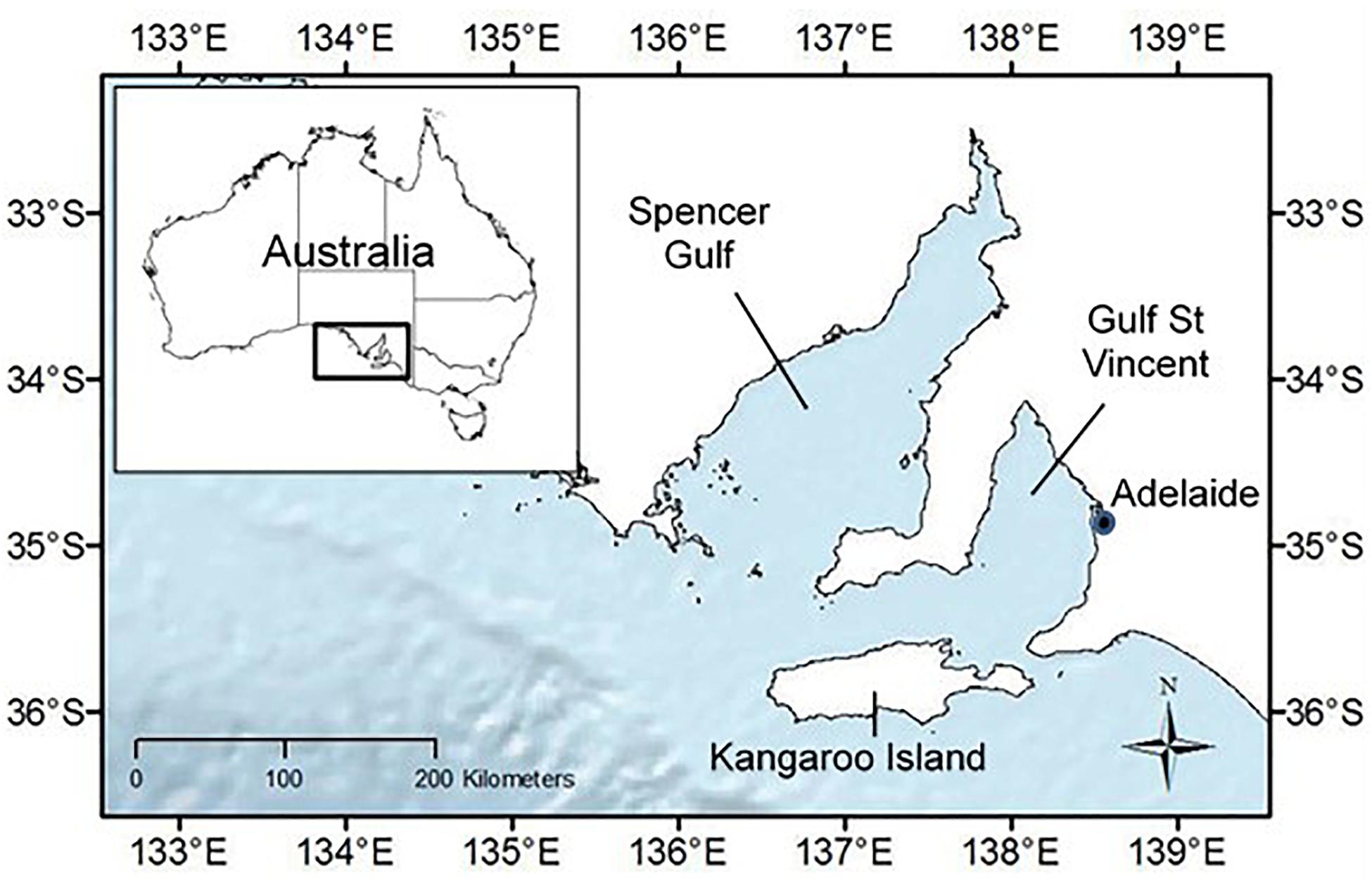
Figure 1. Map of the study regions of Spencer Gulf and Gulf St Vincent located in southern Australia.

Bioenergetics Model

Demographic information was compiled for bottlenose dolphins (Tursiops spp.) from this and other regions to provide the best estimates for parameters that were not available for these two study populations (Table 1). The majority of parameters obtained from surrogates came from coastal populations, providing comparable estimates for the study populations used here. Information on energetics was derived directly from the gulf populations, and surrogate data from other populations or bottlenose dolphin species were used when population specific information was unknown. The bioenergetics model was used to provide the daily energetic requirements for the individuals in the simulations. A growth curve was used to estimate the length and mass of the individual, from which the individuals metabolic rate was derived, with corrections for metabolic efficiency, as well as estimated food intake and energy stores for the individual. Additional energy requirements due to reproduction were included in the energetics model to account for the higher energetic requirements of lactating females.

TABLE 1

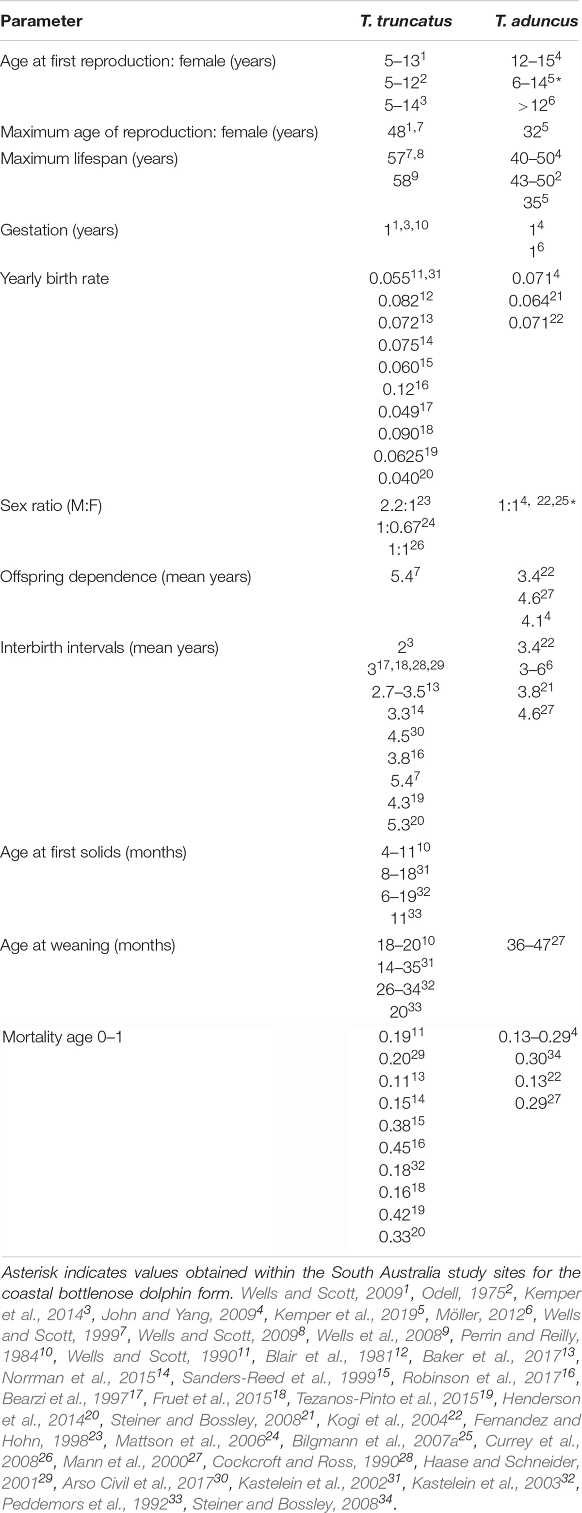
Table 1. Demographic information for bottlenose dolphins used to estimate model parameters that were unknown for the two populations.

Growth Curve

Bioenergetics models require a field metabolic rate (FMR), which can be calculated from a linear relationship with body mass (Kleiber, 1947; Costa and Maresh, 2018). Body mass of individuals is derived from the length of individuals (Eq. 2). Data on female dolphins within the study region in South Australia were obtained from stranding data, and used to develop female growth curves (Kemper et al., 2019). The curves were calculated using the formula:

$$L=a\times exp(-b\times \exp (-\text{c}\times X))(1)$$

where L is an individual’s total length in cm, a is the asymptote where growth begins to plateau, b is the lower asymptote where the slope begins, c is the intrinsic growth rate, and X is the age of the individual in years (for a full list of model parameters see Table 2). Length of individuals was assumed to be distributed normally around the mean, μ_L, with a standard deviation of 10 cm to account for the natural variation in size among individuals of the same age within the population based upon the growth curve (Kemper et al., 2019). The length of the individuals was then converted to body mass using a Tursiops derived model between length and mass (Hart et al., 2013):

TABLE 2

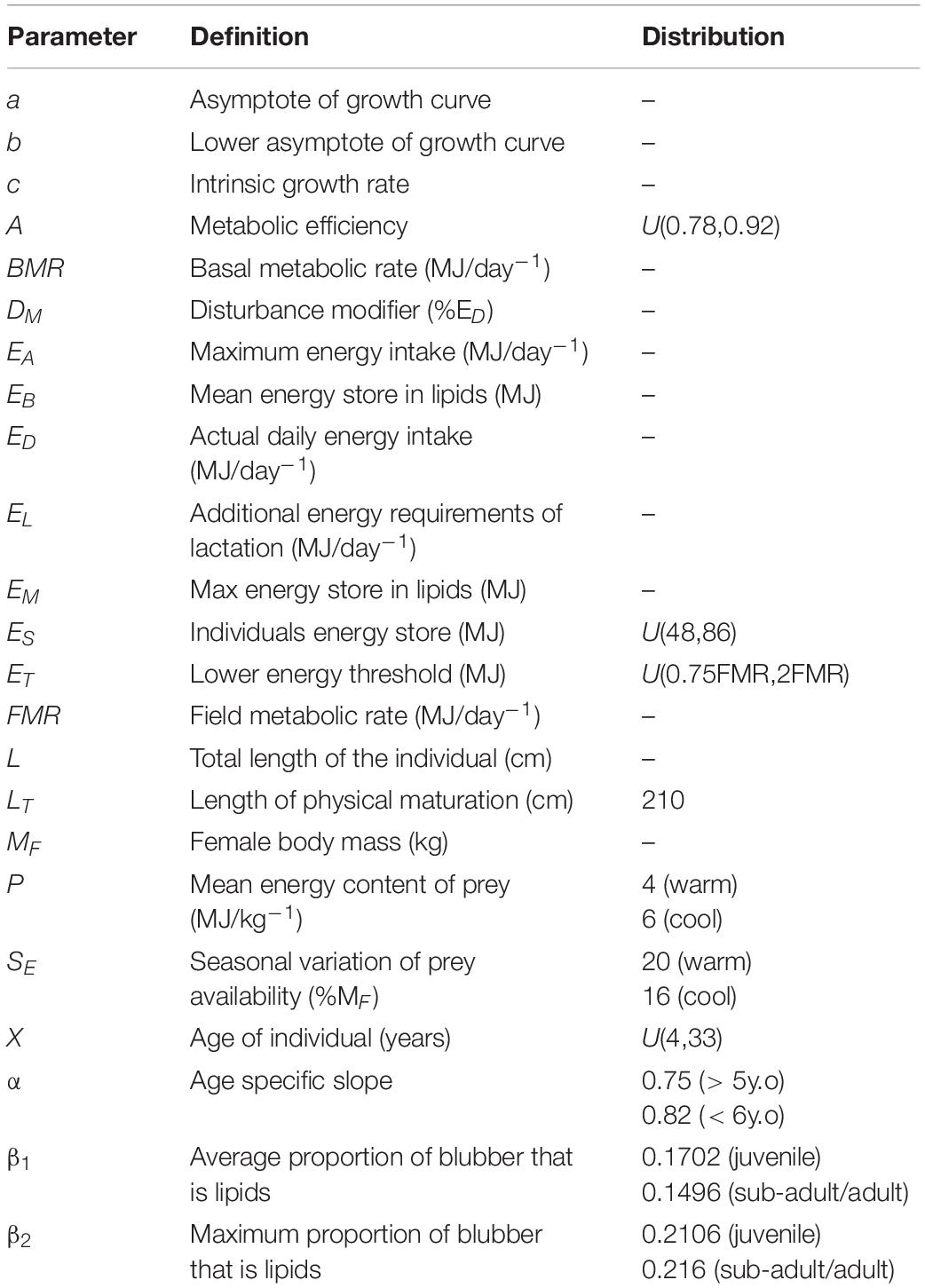
Table 2. List of model parameters, their definition, and the distribution they were sampled from.

$$M_F={10}^{-4.29}\times L^{2.73}(2)$$

where M_F is an individual female’s body mass (kg) and L is her total length (cm).

Energetics

Female body mass from Eq. 2 was used for the calculation of individual basal metabolic rate (BMR, M day^–1) using Kleiber’s Law (Kleiber, 1947):

$$BMR=0.293\times M_F^{\mathrm{\alpha }}(3)$$

where α is the slope (α = 0.75 for individuals 6 years and older, α = 0.82 for individuals younger than six to account for the increased costs associated with growth) (Riek, 2008).

To obtain FMR, a multiplier of 3–6 has been suggested for bottlenose dolphins, though work on the mitochondrial density and lipid content of muscle tissue suggests that bottlenose dolphins actually have a moderate metabolic cost of living compared to other cetacean species (Spitz et al., 2012). Sympatric Australian sea lions (Neophoca cinerea) showed higher BMR during stages of fat accumulation (Ladds et al., 2017a) and the dolphin populations in Sarasota Bay, United States, the population from which the suggested multiplier was derived tend to live in waters with greater yearly variation in temperature than those in southern Australia. This results in greater fluctuations in blubber thickness and composition (11–33°C in Sarasota Bay, United States vs. 14–26°C in Spencer Gulf, South Australia) (Lackenby et al., 2007; Iverson, 2009; Barbieri et al., 2010). Therefore, a multiplier of 2–5 times BMR was used to account for the reduced variability in temperature in southern Australian waters. Given that the exact multiplier is not known, the uncertainty in this value was incorporated by selecting the multiplier from a uniform distribution, U(2, 5), for each female in the population. The addition of this multiplier provides an estimate for the FMR of bottlenose dolphin in southern Australia, consistent with those used for other species (Bejarano et al., 2017; Ladds et al., 2017a,b; Costa and Maresh, 2018).

Metabolic Efficiency

Accounting for the efficiency of energy uptake from food is also required, as not all food that is ingested by individuals is assimilated as energy. Some energy in prey cannot be accessed (e.g., squid beaks), and some is lost as waste through urine and feces. Metabolic efficiency is therefore the percentage of the total potential energy that is actually assimilated by an individual. For bottlenose dolphins the metabolic efficiency of a fish diet, when accounting for fecal waste ranged between 89 and 96% (Reddy et al., 1994). Energy from urinary loss is still unknown for bottlenose dolphins, but in pinnipeds it ranges between 7 and 10% (Keiver et al., 1984; Ronald et al., 1984; Fisher et al., 1992). As a result, these values were used as a proxy in the two dolphin populations, given a uniform 0.78–0.92 [U(0.78, 0.92)] for metabolic efficiency in the model (Bejarano et al., 2017).

Food Intake

Changes in the diet and energy content of prey in dolphins have been seen with warmer months showing a higher density of prey, but reduced quality and size (McCluskey et al., 2016). Habitat modeling from the two gulfs has revealed differences in the seasonal distribution of bottlenose dolphins, with a preference for upper gulf waters during winter/spring (cool season) and coastal waters during summer/autumn (warm season) (Bilgmann et al., 2019). Bottlenose dolphins in Spencer Gulf reportedly exploit the annual mass aggregation of breeding giant cuttlefish (Sepia apama), which occurs during the cooler months (Finn et al., 2009), and stable isotope analysis showed differences between the diet of northern and southern Spencer gulf dolphins (Gibbs et al., 2011). Details of the seasonal differences in diet in southern Australia, however, are not well-understood. Values for the average energy content of prey (P) were taken from studies looking at prey of bottlenose dolphins, giving a mean energy content of 4 MJ/kg used for the warm season, and a value of 6 MJ/kg in the cool season (Spitz et al., 2012; McCluskey et al., 2016). Mean values of prey energy content were consistent with energy densities for prey previously identified in the diet of these dolphin populations (Gibbs et al., 2011). In captive animals, individuals consume on average 2–10% of their body mass in prey daily, though for wild individuals this value is expected to be higher, averaging between 16 and 20% (Kastelein et al., 2000, 2002; Rechsteiner et al., 2013; Srinivasan et al., 2017). Values for seasonal variation of prey availability (S_E) were taken from the variation in daily prey consumption with 20% used for warm season and 16% used for the cool season (Rechsteiner et al., 2013; McCluskey et al., 2016). With the limited information on feeding in wild bottlenose dolphins, a conservative approach was used to estimate the maximum possible energy intake based upon the relationship between proportion of body mass and amount of food required:

$$E_A=M_F{S}_{E}PA(4)$$

where E_A is the maximum possible energy acquisition (MJ/day), and A is the individual metabolic efficiency.

Energy Stores

Bottlenose dolphins, like most marine mammals, have a layer of blubber below their skin which aids in insulation, buoyancy, and locomotion, while also providing a lipid-rich energy store to cope with changes in food availability and reproductive events (Iverson, 2009). In common bottlenose dolphins, blubber stores have been shown to change over development, with sexually mature individuals and juveniles having the highest concentration of stores (Struntz et al., 2004). Information on the proportion of mass composed of blubber was used to estimate the average proportion of body mass that is blubber (Struntz et al., 2004). The average proportion of the blubber that is lipids (β₁) for different age groups was then used to calculate the average energy store for individuals (β₁: for juvenile = 0.1702; for adult and sub-adult = 0.1496).

$$E_B=\frac{{\mathrm{\beta }}_1{M}_F\times 39.42}{2}(5)$$

where E_B is the individual’s mean energy store (MJ). A lipid energy density of 39.42 MJ/kg was used as per Blaxter (1989), which is consistent with other estimates used in marine mammal energetics models (Rechsteiner et al., 2013; Christiansen and Lusseau, 2015; Beltran et al., 2017; Farmer et al., 2018). Not all blubber is accessible as an energy store, so the total potential energy in an individual’s lipids was halved to give the lipid stores, E_S. This decision was based upon studies showing a 50% reduction in lipid content of blubber for emaciated individuals compared to robust individuals, with remaining blubber believed to be structural or serve another purpose such as insulation or streamlining (Koopman et al., 2002; Struntz et al., 2004). A maximum energy store (E_M) was also calculated by means of Eq. 5, using the maximum proportion of mass that was blubber, and the maximum proportion of blubber that was lipids (β₂) instead of β₁ (β₂ for juvenile = 0.2106; and for adults and sub-adults = 0.216) (Struntz et al., 2004).

Reproductive Requirements

Physical maturity in bottlenose dolphins is often associated with the total length of the individual rather than age. For dolphins in the two study populations, physical maturation was set to L = 210 cm based upon the average length of maturity from these populations (Kemper et al., 2019). The model accounts for the changes in energy requirements for lactating females and calves. For lactation, an energy multiplier of 48–86% was applied to FMR for the increased energy requirements of the mother (E_L) (Kastelein et al., 2002, 2003). The energy multiplier was also added to the E_A of lactating individuals over the lactation period to account for the additional food requirements to meet their increased metabolic costs.

Simulations

Each simulation was run over a period of 5 years as a baseline for the influence of disturbances on the populations, with births and conceptions taking place on the first day of each year (January 1), representing the peak birthing period for bottlenose dolphins in these populations, given the average 12 month gestation period. Seasonal differences in prey quality were incorporated with the inclusion of two seasons, changing from a warm season to a cool season halfway through each year. Individual E_S was set to the mean energy store in lipids (E_B) at the start of the simulation. For each day in the simulation, E_D was derived for each individual, with the flow of energy determined by the reproductive state of the individual and previous energy intakes and available energy stores (Figure 2). Yearly growth was determined by the proportional difference in the yearly average between E_S and E_B, with individuals acquiring more energy growing proportionally more, and individuals acquiring less energy growing proportionally less than average for their age. Lactating individuals who died during the simulation also lost their calf, an assumption based upon the calf’s high maternal dependency. Natural mortality rates (μ_m = 0.024, σ_m = 0.0198) were applied to the populations to account for predation and illness, as well as an increased mortality rate (0.35) for individuals over the age of 35 years to account for uncertainty in the maximum age of bottlenose dolphins in the populations.

FIGURE 2

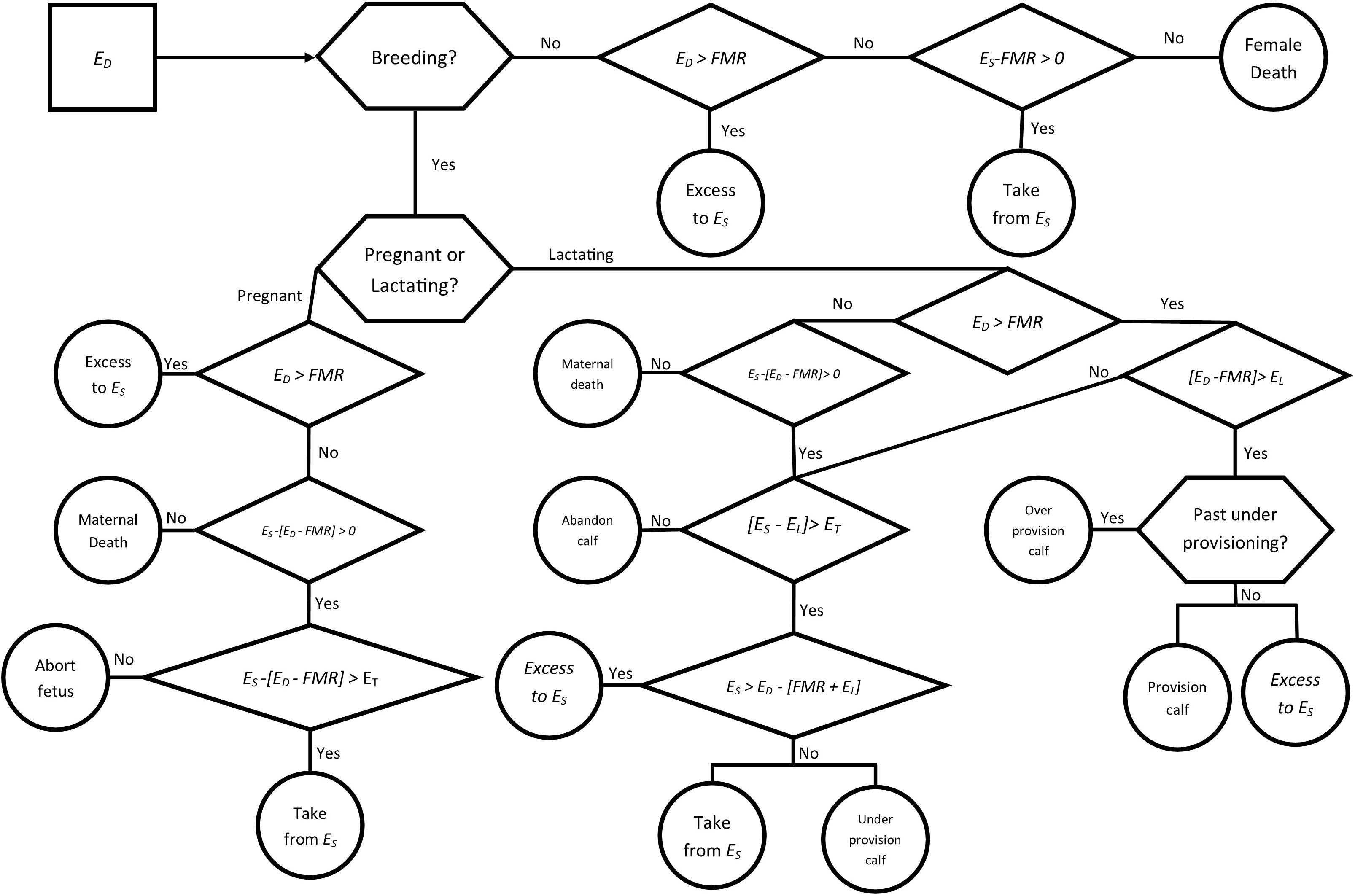
Figure 2. Decision tree representing a single time step (1 day) in the model for an adult female bottlenose dolphin. Ingested energy (E_D) is acquired by an individual each day, the use of that energy varies depending on the reproductive status of the female.

To account for heterogeneity of individuals within the population, ages for individuals were drawn at random between age after weaning (4 years) and expected maximum age (32 years) based upon known information on bottlenose dolphin population age structure (Stolen and Barlow, 2003; Mattson et al., 2006). The age was then used to calculate the length (Eq. 1) and the mass (Eq. 2) for each individual within the population. BMR for individuals was calculated based upon their mass (Eq. 3), which was then converted to provide the FMR for each individual. A 4 year average interbirth interval was assumed for the population (Kemper et al., 2019) (Table 1), with the reproductive status of females at the beginning of the simulation distributed evenly between pregnant, reproductively active and the stages of lactation (first, second, or third year) for individuals greater than 210 cm in length.

To account for natural variation in prey availability, energy intake was incorporated by drawing an individual’s daily food intake (E_D) taken from a normal distribution centered on a mean of E_A (Eq. 4). For lactating individuals the additional energy costs of lactation (E_L) were applied from the date of their calf’s birth until 11 months after birth, when the calf begins to forage independently (Table 1) (Peddemors et al., 1992; Kastelein et al., 2002, 2003). From month 11 the additional energy cost to lactating mothers was decreased linearly until the start of month 28 when the mother ceased lactation and the calf was presumed weaned (Table 1). For the calves that weaned, half were assumed to be female, with the remainder male. Female calves were added to the population after weaning as a juvenile individual, independent from their mother. For each day in the simulation, E_D was calculated for each individual and values greater than energy requirements of FMR were considered to result in an energy surplus, which could be used for the E_L for lactating individuals, or added to the energy store, E_S. On days when E_D was below the energy requirements, the required energy could be metabolized from E_S, with values for E_S below zero resulting in the death of the individual.

Females were assumed to have a lower energy store threshold (E_T) which was drawn from an uniform distribution with a lower limit equal to three-quarters of the FMR and the upper limit equal to twice the FMR, U(0.75FMR, 2FMR), for each individual. For lactating and pregnant females, if the threshold value was reached, individuals were assumed to prioritize their own survival and abandon the calf or abort the fetus. Lactating females used surplus energy to provision the calf, with any remaining added to E_S. As females were assumed to prioritize their own survival, if a lactating female was forced to metabolize energy from her E_S to meet her own needs, she would only fully provision to the calf if her stores were greater than her FMR and the cost of lactation E_L, otherwise the calf would be under provisioned. Calves that were under provisioned incurred a higher chance of mortality based upon the proportion of their energy intake over the year that they did not acquire from their mothers and could not otherwise mitigate for.

Using the model structure described above (Figure 2), both dolphin populations were simulated using the statistical programming language R version 3.5.3 (R Core Team, 2017). Individual components of the model were designed as user defined functions, and applied to individuals within the population for each simulated day to determine the flow of energy. The simulations were performed to assess the population dynamics under no disturbance scenario and with the inclusion of disturbances (described below) to compare potential impacts, with 1000 iterations of the 5 year period performed for each scenario. The simulation outcomes were checked at each stage of the model to ensure representative output based upon the population parameters and expected influences of disturbances.

Disturbance Scenarios

The disturbances explored were those considered the most likely to impact bottlenose dolphins in South Australian populations, based upon Robbins et al. (2017). The fourth, a morbillivirus outbreak, was included due to its history in southern Australia and prevalence in marine mammals (Van Bressem et al., 2014; Kemper et al., 2016). The scenarios consisted of a baseline scenario with no disturbances, and disturbance scenarios as follows: four climate change scenarios of differing intensities, one fisheries related mortality scenario, one habitat disturbance, and four epizootic scenarios using differing frequencies/impact combinations. Each scenario was applied to both the Spencer Gulf and Gulf St Vincent dolphin populations with the estimate of the intensity of disturbance estimates specific for each gulf. Disturbances were incorporated either as a reduction in food availability in the climate change and habitat disturbance scenarios, or as changes in individual mortality for fisheries interactions and epizootic scenarios (Figure 3). Affected individuals were selected randomly from the population in each simulation, regardless of age or reproductive status.

FIGURE 3

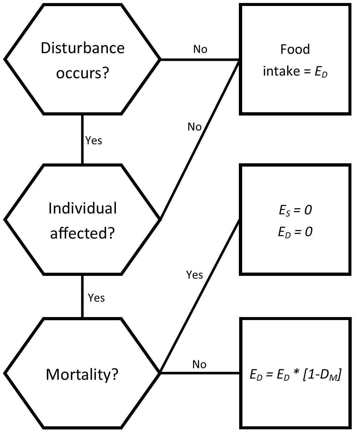
Figure 3. Decision tree for how individuals are impacted by a disturbance for each time step (1 day). Disturbances influence the daily energy intake (E_D) of an individual that is affected, while influencing both the energy intake and energy store (E_S) of individuals who die as a result of disturbances.

Climate change

Climate change was considered the disturbance most likely to impact the bottlenose dolphins within the gulfs and was assumed to include issues such as changes to temperature, frequency of storm activity, ocean acidification and warming, as well as increases in salinity. These shifts in climate can lead to changes in dolphin dispersal based upon thermal tolerances and fluctuations in survival and reproduction in extreme heatwave events, as well as variation in prey distribution and availability (Schumann et al., 2013; Wild et al., 2019). Four climate change scenarios were considered for each population and were based upon historic sea surface temperature (SST) anomalies for the region from 1998 to 2018, SST data was sourced from the Integrated Marine Observing System (IMOS, 2019), which is a national collaborative research infrastructure, supported by the Australian Government. The four scenarios consisted of low (a warming event one anomaly higher than expected), moderate (a warming event two anomalies higher than expected), high (a warming event three anomalies higher than expected) and extreme (a severe heatwave). Frequency of occurrence for each event was based upon the SST anomalies and physical characteristics of each gulf. Each monthly anomaly from the historic data was recorded and the probability of occurrence calculated from their frequency over the past 20 years for each gulf. The chances of an event occurring in a given year for Spencer Gulf were 100% for low, 90% for moderate and 25% for high; while for Gulf St Vincent 100% for low, 85% for moderate and 15% for high. The chance of extreme events was set at 50% for both populations to simulate the potential effect of increased likelihood of heat events on the populations, with the potential high frequency of extreme events resulting from climate change. The chances for the first three of the four scenarios therefore differed between the two gulfs, while the chances for the fourth were the same. Changes in prey availability occurred with changes in ocean temperature through the addition of a disturbance modifier (D_M) that defined the percentage reduction in prey available to an individual. Extreme and high events incurred a D_M of 25–35% reduction in food, moderate a 15–25% reduction, and low a 0–15% reduction. The D_M was applied to all individuals within the population, with the value for the reduction being drawn from a uniform distribution for each individual on each day of the simulated year.

Habitat disturbance

This scenario focused on the impacts of shipping with the associated impacts of noise pollution on the populations. Information on the likelihood of individual dolphins being affected were derived from population density maps (Bilgmann et al., 2019), as well as yearly ship traffic densities for each of the gulfs. The proportions of each population likely to be affected differed. A total of 10–30% of individuals in Gulf St Vincent, and 10–20% of individuals in Spencer Gulf were assumed to be affected on each day of the simulation, with the proportion drawn randomly each day. We assumed that those individuals affected by this disturbance would experience reduced foraging ability, resulting in a D_M of 5–30%, reducing food intake for each individual, drawn randomly from a uniform distribution.

Fisheries interactions

Interactions between bottlenose dolphins and fisheries within the South Australian gulfs and adjacent state and federal waters have long been reported (Kemper et al., 2005). Though the incidence of reported interactions in the two gulfs are low, there are still likely to be mortalities resulting from fisheries bycatch, particularly within the haul and gillnet fisheries (Robbins et al., 2017). Based upon population density maps and information on reported dolphin bycatch mortalities with dolphins within the gulfs, we estimated 5% of the Gulf St Vincent population came into contact with fisheries during the warm season, and 20% during the cool season; for Spencer Gulf, 15% during the warm season and 5% during the cool season (Mackay et al., 2017; Bilgmann et al., 2019). For those individuals that came into contact with fisheries, 0–2% of the Gulf St Vincent population and 0–5% of the Spencer Gulf population would have a fatal interaction based upon the different fishing intensities within each gulf (Mackay et al., 2017; Bilgmann et al., 2019). This was a conservative approach based on current fishing methods and distribution of fisheries, and no scenarios investigated the potential for increased bottlenose dolphin–fishery interactions resulting from possible changes in any of the fisheries management or implementation.

Epizootic

Epizootic events have been recorded in southern Australia, with an outbreak of cetacean morbillivirus having occurred in Gulf St Vincent in 2013 (Kemper et al., 2016). Information on the patterns of morbillivirus outbreaks are largely unknown, and there is variability in the geographical extent, mortality rate and duration (Van Bressem et al., 2014). In the Mediterranean there have been three morbillivirus events separated by an average period of 11 years (Raga et al., 2008). Four scenarios for each gulf were simulated, looking at two levels of intensity and frequency. Low intensity events resulted in 15% mortality in the population, and high intensity events resulted in 50% mortality in the population. Mortalities were modeled as a loss of foraging and energy stores for the individuals affected during the simulation (Figure 3). Changes in the frequency of the events were gulf specific, with Gulf St Vincent experiencing a low frequency with a probability of once every 11 years, and a high intensity event once every 5 years. Frequency of occurrence for Gulf St Vincent was doubled for Spencer Gulf (22 years) due to no known records of cetacean morbillivirus outbreaks within this gulf.

Results

Differences in abundance and fecundity from modeled scenarios were compared to the base scenario, were no disturbances were modeled, thereby accounting for natural variation in survival and fecundity within the populations. Comparisons between scenarios were made to the base scenario to understand the extent of potential disturbances.

Abundance

The base scenario showed little variation in the estimated mean population size for both populations, the larger Spencer Gulf and the smaller Gulf St Vincent population over the 5 year simulation (Figure 4). Epizootic events of a high intensity had the largest impact on both populations regardless of frequency. High intensity, high frequency epizootic events saw a 43% decline in the Spencer Gulf population (N = 622, bootstrap CI = 118–1146), compared to a 23% decline in the Gulf St Vincent population (N = 366, bootstrap CI = 109–508), over the 5 year period (Figure 4). A reduction in the frequency of the high intensity epizootic events saw an intermediate reduction in abundance for both populations, with a 21% decline in Spencer Gulf (N = 878, bootstrap CI = 263–1166), and a 12% decline in Gulf St Vincent (N = 424, bootstrap CI = 198–511) (Figure 4). Scenarios containing low intensity epizootic events had little influence on the abundance of either population over the simulated period (Figure 4).

FIGURE 4

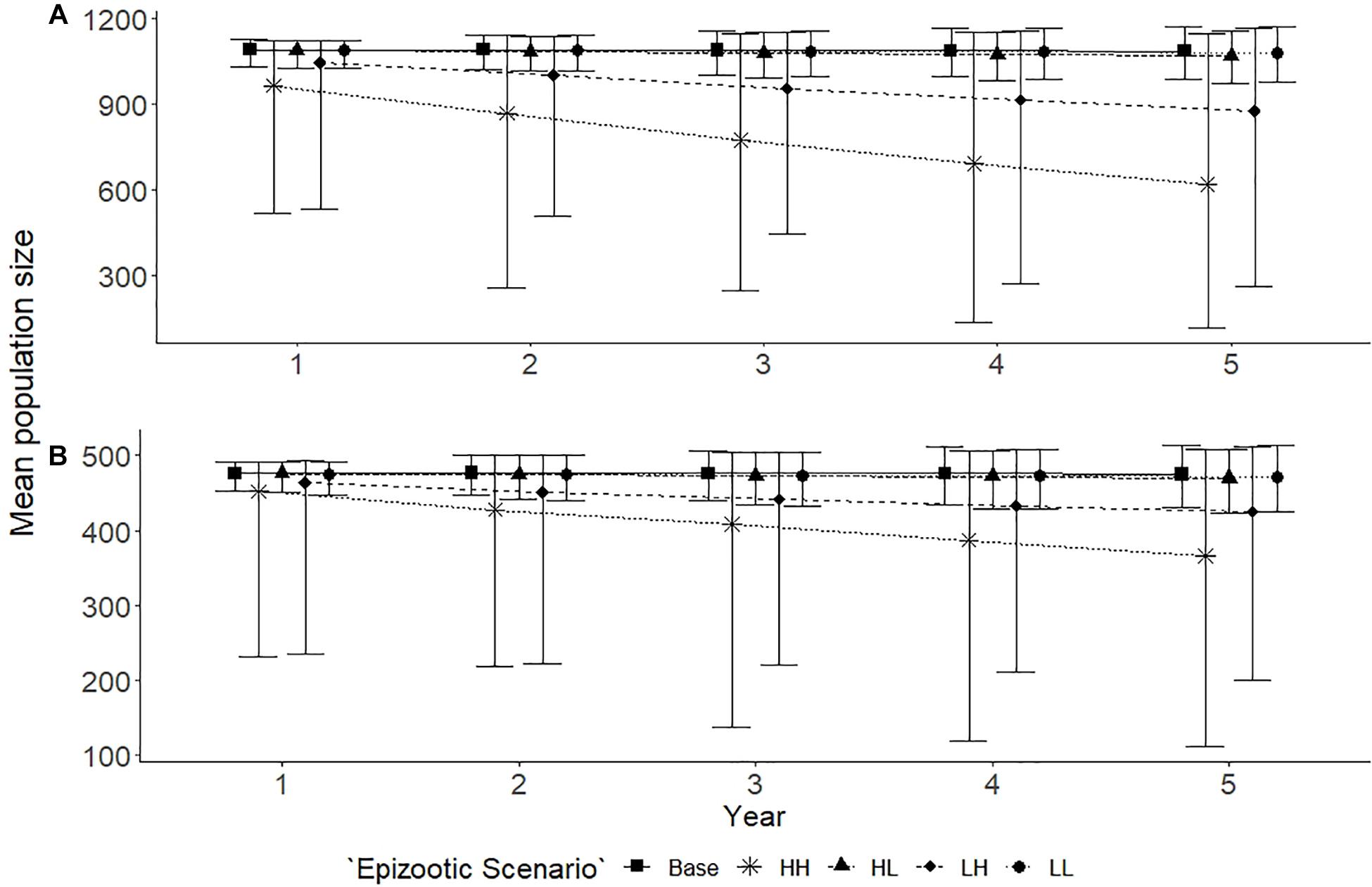
Figure 4. Population trends for Spencer Gulf (A) and Gulf St Vincent (B) with epizootic scenarios, predicted over a 5 year period. Five scenarios are examined for each population: base with no disturbances (■); high frequency and high impact [HH] (∗); high frequency and low impact [HL] (▲); low frequency and high impact [LH] (◆); and a low frequency and low impact [LL] (•). Scenarios resulted in mortalities for individuals affected, with the level of impact determining the proportion of the population affected. Points indicate the mean and error bars indicate standard deviation of the simulations.

Abundance estimates varied slightly in the climate change scenarios in both populations (Figure 5). In the extreme scenario, for both the Spencer Gulf (Figure 5A) and Gulf St Vincent (Figure 5B) populations, there was a 6% decline in the mean population size (Spencer Gulf: N = 1017, bootstrap CI = 710–1151; Gulf St Vincent: N = 449, bootstrap CI = 303–504) over the 5 year simulation period. The variation in the extreme scenarios for both populations were high, particularly the lower bound of the confidence intervals, showing the potential range of impacts for these populations (Figure 5). High, moderate and low scenarios saw less than a 5% change in abundance for both populations over the 5 year simulation.

FIGURE 5

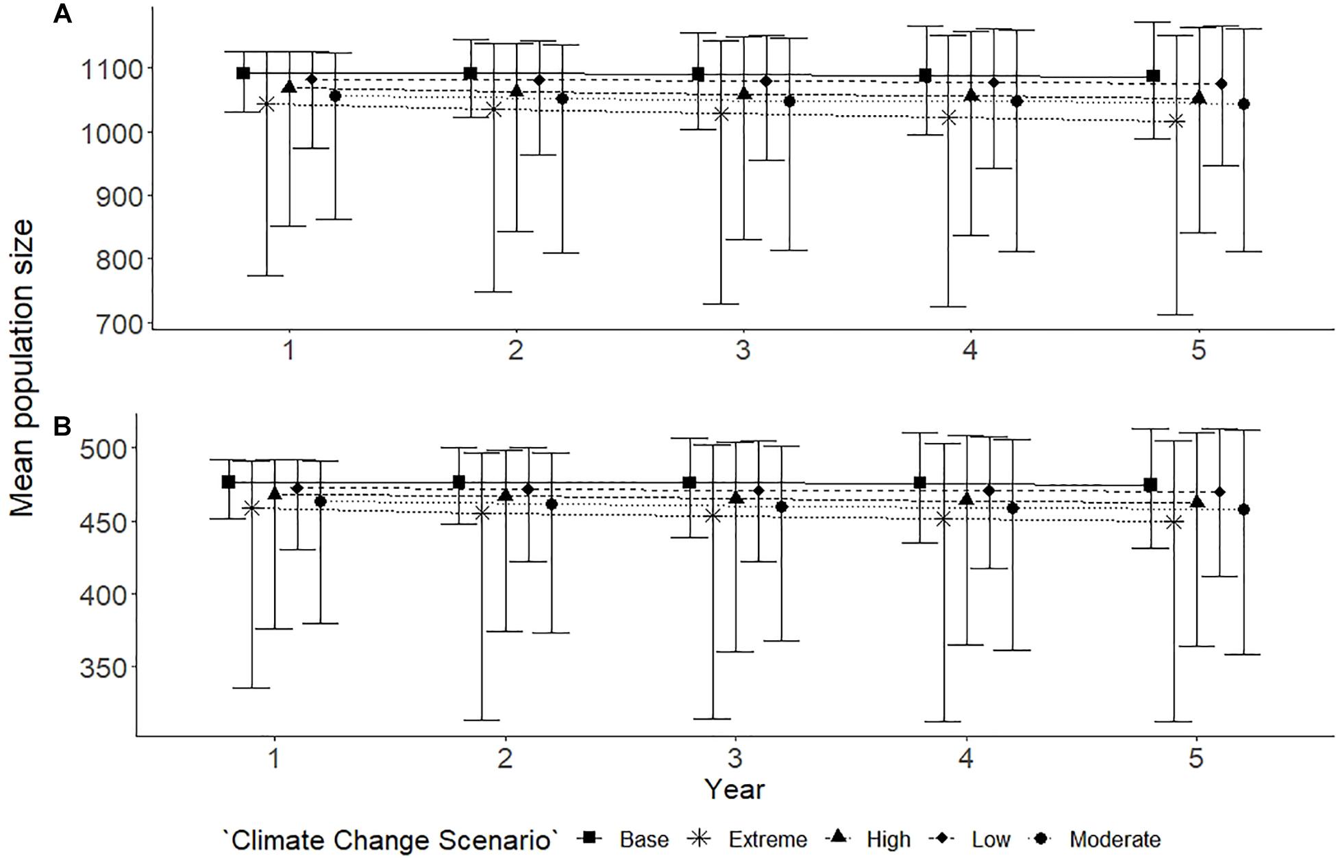
Figure 5. Population trends for Spencer Gulf (A) and Gulf St Vincent (B) under climate change scenarios, predicted over a 5 year period. Five scenarios were examined for each population: base with no disturbances (■); extreme climate scenario (∗); high climate scenario (▲); moderate climate scenario (•); and a low climate scenario (◆). Scenarios had varying probabilities of occurrence based upon historic climate events and resulted in a proportional reduction in food increasing with severity. Points indicate the mean and error bars indicate standard deviation of the simulations.

Fisheries interactions and habitat disturbance scenarios showed little variation in abundance over the 5 year simulation when compared to the base scenario (Figures 1, 2 and Supplementary Figure 1).

Fecundity

Changes in fecundity were recorded as changes the number of failed pregnancies, calves born, calves abandoned and calves successfully weaned during the simulations. High frequency, high intensity epizootic outbreaks were seen to have the biggest influence on breeding success for both populations, with low frequency and high intensity having the second biggest influence (Figure 6). High intensity scenarios showed an increase in the number of failed pregnancies for both populations, with Spencer Gulf having a 3.8 and 2.5 times increase from base scenarios for high and low intensity (Figure 6A), while Gulf St Vincent showed a 2.4 and 1.9 times increase for high and low intensity, respectively (Figure 6E). Low intensity scenarios resulted in a change of less than 10% in the number of failed pregnancies compared to base scenarios for both populations (Figures 6A,E). Of the climate change scenarios, extreme scenarios showed the greatest influence on successful breeding for both populations, with over a 1.7 times increase in the number of failed pregnancies in Gulf St Vincent (Figure 7E), and an increase of over 1.8 times for Spencer Gulf compared to base scenario (Figure 7A). Changes in the number of failed pregnancies were also seen in other climate change simulations with Spencer Gulf seeing a 1.4, 1.6, and 1.2 times increase for high, moderate and low scenarios, respectively (Figure 7A), while Gulf St Vincent saw a 1.3, 1.6, and 1.2 times increase (Figure 7E).

FIGURE 6

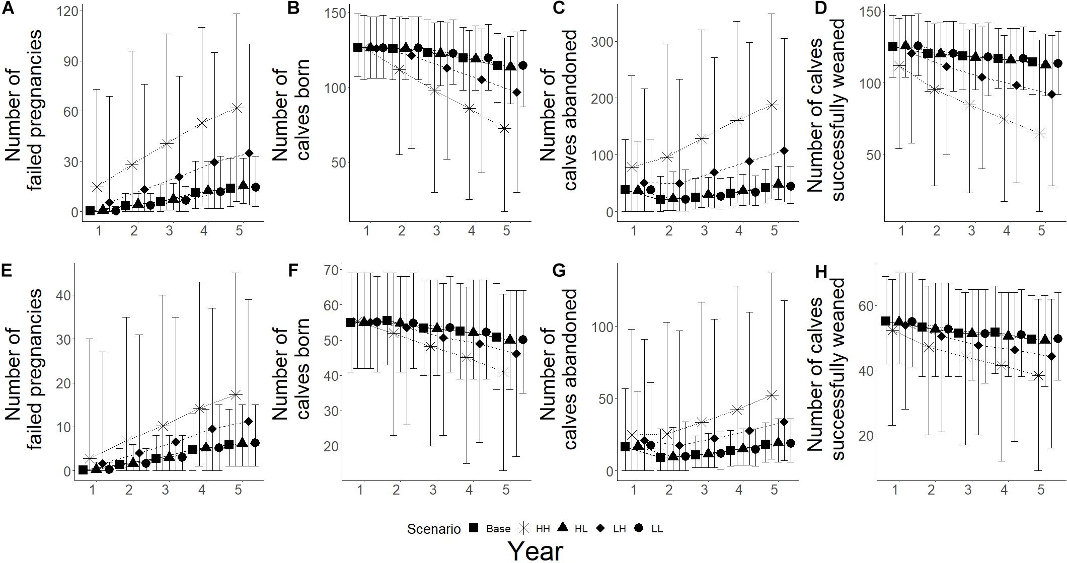
Figure 6. Reproductive parameters under epizootic simulations for both populations. Five scenarios presented with base (■), HH – high frequency/high impact (∗), HL – high frequency/low impact (▲), LH – low frequency/high impact (◆), and LL – low frequency/low impact (•). (A–D) Represents Spencer Gulf, (E–H) represents Gulf St Vincent. (A,E) Shows the mean number of failed pregnancies for each scenario; figures (B,F) show mean number of calves born; (C,G) shows the mean number of abandoned calves; and (D,H) shows the mean number of calves that survived to weaning.

FIGURE 7

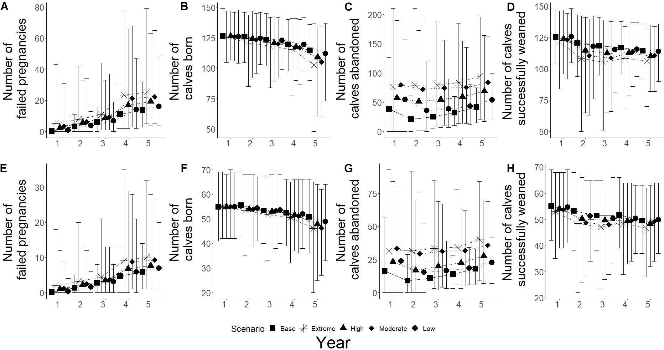
Figure 7. Reproductive parameters under climate simulations for both populations. Five scenarios presented with base (■), extreme (∗), high (▲), moderate (◆), and low (•). (A–D) Represents Spencer Gulf, (E–H) represents Gulf St Vincent. (A,E) Shows the mean number of failed pregnancies for each scenario; figures (B,F) show mean number of calves born; (C,G) shows the mean number of abandoned calves; and (D,H) show the mean number of calves that survived to weaning.

The number of calves born was reduced by 35% in Spencer Gulf (Figure 6B), and 16% in Gulf St Vincent (Figure 6F) in the high frequency, high intensity epizootic scenarios. High intensity, low frequency epizootic events had the second largest influence on the number of calves born for both populations, with a 16% decline in Spencer Gulf (Figure 6C), and a 9% decrease in Gulf St Vincent (Figure 6F). Changes in calving were also seen during the extreme climate change scenarios for both Spencer Gulf and Gulf St Vincent, with a 10 and 9% reduction, respectively (Figures 7B,F). Changes in birth rates for Spencer Gulf showed a 5, 8, and 2% decrease, while Gulf St Vincent saw a 6, 9, and 4% decrease in the high, moderate and low scenarios, respectively (Figures 7B,F).

Epizootic scenarios of high intensity were seen to have the largest influence on the number of calves abandoned, with a 3.5 and 2.6 times increase in Spencer Gulf (Figure 6C), and a 2.3 and 1.8 times increase in Gulf St Vincent (Figure 6G) for high and low frequency, respectively. In climate change scenarios the rate of calf abandonment was highest in extreme scenarios with a 2.3 times increase in Spencer Gulf (Figure 7C), and a 2.2 times increase in Gulf St Vincent (Figure 7G). Moderate climate change scenarios saw 2 times the number of calves abandoned compared to the base scenario for both populations (Figures 7C,G). High and low scenarios had a 1.5 and 1.3 times increase for Gulf St Vincent and a 1.7 and 1.3 times increase for Spencer Gulf, respectively (Figures 7C,G).

The number of calves successfully weaned was most influenced by high intensity epizootic events, with a 43 and 35% decrease in Spencer Gulf (Figure 6D), and a 23 and 10% decrease in Gulf St Vincent (Figure 6H) for high and low frequency, respectively. Low impact epizootic scenario saw a less than 5% change from base scenarios regarding weaning success (Figure 6). The number of calves weaned showed a decrease in Spencer Gulf of 7, 4, and 3% in the extreme, high and moderate climate change scenarios respectively, compared to the base scenario (Figure 7D), while in Gulf St Vincent showed a decrease of 6 and 2% in the extreme and high scenarios (Figure 7H).

Fisheries interaction and habitat disturbance scenarios saw little change in the number of failed pregnancies, calves born, abandoned or successfully weaned over the 5 year period when compared to the base scenario (Figure 3 and Supplementary Figure 1).

Discussion

Current knowledge of population size, life history traits and energetics of bottlenose dolphins in two South Australian gulfs was used to develop a model that explored how current threats would likely influence the abundance and reproduction of two geographically isolated and genetically distinct populations. In this study, we modeled the populations for a 5 year period to understand the potential effects of these disturbances over a small time scale, especially given that the impact and extent of these disturbances is highly uncertain and likely to change in the near future (Robbins et al., 2017). We found that epizootic and climate change scenarios were likely to have the greatest influence on both populations over the modeled time period.

Epizootic events of a high intensity had the greatest influence on population size and reproductive parameters for both populations, regardless of the frequency of the events. High intensity scenarios were shown to have wide variation in the output for both the high and low frequency scenarios. The impact of morbillivirus outbreaks globally shows varied impacts both between populations and species, with some events resulting in mortality of more than half the population (Guardo et al., 2005). The frequency of such events and whether they may increase within populations stressed by other factors such as temperature changes remains to be seen. However, environmental variables such as reduced prey availability, higher than average SSTs and toxic contamination, as well as population densities are predicted to play a role in the frequency of outbreaks of infectious diseases such as morbillivirus (Van Bressem et al., 2014; Kemper et al., 2016).

Climate change was ranked as the biggest threat facing bottlenose dolphins in Spencer Gulf through expert elicitation (Robbins et al., 2017). Our results suggest that extreme climate change scenarios have the third largest influence on both abundance and fecundity, after high intensity epizootic events, for both gulfs. The model results are comparable to the reported changes in survival following an extreme heatwave event in Western Australia that resulted in a 5.9–12.2% decline in the abundance of bottlenose dolphins (Wild et al., 2019). The reduction in food availability modeled as part of these scenarios likely drives these results, with increased metabolic need, especially for lactating females, leading to reduced reproductive success, something seen in the natural population post-heatwave in Western Australia (Wild et al., 2019). The four modeled scenarios focusing on climate impacts showed wide variation in simulation output, due in part to our uncertainty in how these ecosystems will respond to climate change events, how severe these events may be, and what impact this will have on prey in southern Australian waters. Climate change is likely to affect bottlenose dolphins by changing the abundance and distribution of prey, as extreme events result in major loss of seagrass, which provides habitat for many of their prey species (Thomson et al., 2015). While these extreme climatic events have been shown to impact some populations, others show stable population trends following these events, with factors such as habitat range and preference playing an important role (Sprogis et al., 2018). Physical characteristics of the two South Australian gulfs, including negligible freshwater inflow (inverse estuaries), shallow depths, and their limited outflow makes these environments vulnerable to the effects of climate change, potentially leading to the amplification of their effects with rises in ocean temperatures, increased heatwaves, and increases in salinity (Nunes and Lennon, 1986; Petrusevics et al., 2009). Habitat modeling for bottlenose dolphins in South Australia’s gulfs reveal preferences for shallow, coastal waters, similar to other populations of coastal bottlenose dolphins globally; habitats most vulnerable to climate change due to their physical characteristics (Simon and Emer, 2002; Torres et al., 2003; Bilgmann et al., 2019). Community dynamics of seagrass have also been shown to be affected by changes in extreme temperature events, with areas being dominated by early successional species post-heatwave, leading to changes in ecosystem functions (Nowicki et al., 2017). Information on the habitat and abundance of prey species and their response to changing climatic conditions is important to further understand how climate change could influence bottlenose dolphins living in southern Australian waters.

Modeling two, similar, but different sized populations provided insights into how a species may respond to disturbances of differing intensities, whilst simultaneously considering the influence population size may play in the mitigation of disturbances. For all modeled scenarios, the resulting estimates of abundance and fecundity were comparable between the two populations, except for one of the epizootic scenarios, where high impact scenarios had a greater influence on the Spencer Gulf population compared to Gulf St Vincent. The high intensity scenario represents a severe outbreak, affecting half the population and subsequent mortality. In the larger Spencer Gulf population, the effect of the high intensity scenarios was more noticeable, influencing changes in fecundity, and reducing the number of reproductive females within the population. Reproductive output is critical to population viability, comparable to survival, even in slow growing species such as bottlenose dolphins (Manlik et al., 2016). Understanding reproduction and how it may be affected by disturbances and management strategies can provide insight into medium and long term population trends (Manlik et al., 2016). The other scenarios showed little differences in the trajectories between the two populations of different size, in differing habitats and with partly differing severity of disturbances (i.e., higher boat traffic in Gulf St Vincent, increased fisheries interactions in Spencer Gulf). This reveals that both populations may be large enough to react similarly to a number of threats, but it is expected that below a certain size threshold a population would show disparate trajectories leading to a faster decline, especially when effects of inbreeding are also considered (e.g., Reid-Anderson et al., 2019). Inbreeding was not accounted for in any of the models here due to the relatively large population sizes and the assumption of random mating within the population. Furthermore, differences in habitat and sizes of the two gulfs were only indirectly modeled via differing effects of climate change and disease outbreak scenarios on the two populations. Future state-spaced PCoD modeling based on bottlenose density maps derived from aerial surveys in combination with habitat modeling in the two gulfs (Bilgmann et al., 2019) may lead to a better understanding of the influence of habitat type on threat outcomes, especially when threats and dolphin distribution overlap in space and time (e.g., boat traffic, fishery interactions, enhanced coastal effects as a result of climate change, and other factors).

The models described in this study investigated the potential impact of different disturbances on two populations of bottlenose dolphins in isolation. The likelihood of a single disturbance occurring in isolation is unlikely, and many of the scenarios investigated here are likely to influence the intensity and responses of the others, as well as being amplified by other environmental and physical pressures. Epizootic events, such as morbillivirus, have been linked to increases in ocean temperatures (Van Bressem et al., 2014). Disturbances such as fisheries interactions, noise pollution and shipping, which had no influence on the populations when modeled in our simulations, could have synergistic effects when combined with multiple stressors. Assessment of the interaction of multiple stressors on populations can provide insight into their cumulative effects, but also offer a greater range of uncertainty due to the complex nature of these interactions (National Academies Of Sciences Engineering And Medicine, 2017). A modified approach to the PCoD framework, the Population Consequences of Multiple Stressors (PCoMS) could be used to look at the impact of multiple disturbances by taking the temporal and spatial distribution of populations and stressors to investigate their impacts on populations (National Academies Of Sciences Engineering And Medicine, 2017).

The variation seen within scenarios, especially the extremes, represents uncertainty in how these populations may respond to a given disturbance. The level of variation seen in the extreme scenarios could be explained by the intensity of the disturbance paired with the frequency at which they occur. This was compounded by a substantial individual variation, with reproductively active individuals having a greater influence on the population trajectory. When pregnant or lactating females were affected, there were increased rates of failed pregnancies and lower calf survival, directly affecting the population dynamics. The variation in the simulations reflects the many uncertainties in our model, both reducible and aleatory, and represents a distribution of potential outcomes for the two dolphin populations when faced with disturbances of different frequency and intensity, allowing for their precautionary interpretation for management (Pirotta et al., 2018). Rather than using detailed numbers of the trajectories, the magnitude of changes in the general trend over the modeled time period, among the different scenarios, allowed for a ranking of threats as follows: (1) High impact, high intensity epizootic; (2) High impact, low intensity epizootic; (3) Extreme climate change; (4) Moderate climate change; (5) High climate change; (6) Low climate change; (7) Low impact, high intensity epizootic; (8) Low impact, low intensity epizootic; (9) Habitat disturbance; and (10) Fisheries interactions. Modeling of threat impacts over longer time periods, beyond the 5 years used here, could change some of these rankings, for example if threats cause chronic impacts on female fecundity leading to long-term effects on reproductive output.

Many species are under increasing pressure from anthropogenic disturbance, whether it is from climate change, habitat modification and loss, noise pollution or disease outbreaks. Research and management are important tools to understand and protect populations and species affected. In this case study, mean changes in population trends and reproductive parameters were presented in order to provide insight into how these disturbances could affect two bottlenose dolphin populations. Extreme events were seen to have the greatest influence on the population trends and reproduction of dolphins during simulations. The understanding that different species may respond differently to the same disturbance is widely accepted, but differences in the context in which a disturbance occurs may also lead to a large variation of responses within a species (Harding et al., 2019; Radford et al., 2019). Modeled scenarios rely heavily on the choice of input parameters, which were carefully chosen either from the study population itself or from similar proxy populations, but these are only approximations of what may occur in real populations. For example, abundance estimates from seasonal line-transect distance sampling surveys were used (Bilgmann et al., 2019), and mean abundance values across seasons were chosen as starting points for the simulations rather than seasonal values or their upper or lower confidence intervals. We assumed an equal sex ratio in both populations based on previous investigations of sex ratios during genetic sampling (Bilgmann et al., 2007a) and based on what is known from other bottlenose dolphin populations (Kogi et al., 2004; John and Yang, 2009). Any significant deviation from a 1:1 ratio of males and females, would impact model outcomes as it would change the number of females modeled in the population and the resulting reproductive output. Uncertainties in some of the input parameters were modeled using random draws from a uniform distribution, thus incorporating levels of uncertainty in the model output and so making them more tolerant to deviations from a chosen fixed input parameter. Overall, PCoD modeling that applies an integrated bioenergetics model such as the one used here, is a sophisticated, detailed and complex Bayesian modeling approach that is powerful and innovative.

The model used here is a simplified representation of the bioenergetic requirements of bottlenose dolphins, and how disturbances may influence these requirements. Increased information on population specific parameters, as well as predicted disturbances, could be included into the model in the future to assess specific events and provide a clearer representation of these populations. The incorporation of population densities into future models, and how these densities differ within and between the two gulf populations could provide further insight into how disturbances such as epizootic events, which can be exacerbated by large population densities, may influence survival and fecundity. Group dynamics, and the fission-fusion nature of dolphin social groups is an important consideration for future models, as it could have influences in habitat use, food availability and the transmission of diseases. PCoD models are computationally expensive and complex, and relevant considerations need to be made when considering appropriate parameters to include.

To better understand such complex models, population differences including abundance, habitat quality, and genetic variation need to be considered to understand how and why different populations may vary in their responses to disturbances. Individual differences in behavior and physiology, such as thermal tolerance, habituation, local genetic adaptation and immune response are important to consider when interpreting simulation results applicable to population management. Informed management of marine species is required to mitigate the effects of disturbances on populations. Modeling provides a powerful tool to understand how potential disturbances may impact a population, either before they occur or while there is still time to act.

Data Availability Statement

The datasets generated for this study are available on request to the corresponding author.

Author Contributions

JR wrote the manuscript and conducted the modeling. LN aided in model formation and design. KB and RH provided guidance on species biology and site information. KB, RH, and LN revised and reviewed the manuscript. All authors designed the study.

Funding

JR was supported by a Macquarie University Masters of Research scholarship.

Conflict of Interest

The authors declare that the research was conducted in the absence of any commercial or financial relationships that could be construed as a potential conflict of interest.

Acknowledgments

We thank Dr. Peter Corkeron and Associate Professor Rochelle Constantine for their comments and feedback on an earlier draft. Thanks to Macquarie University for providing funding for LN to visit Sydney, thereby instigating this study.

Supplementary Material

The Supplementary Material for this article can be found online at: https://www.frontiersin.org/articles/10.3389/fmars.2020.519845/full#supplementary-material

References

Arso Civil, M., Cheney, B., Quick, N. J., Thompson, P. M., and Hammond, P. S. (2017). A new approach to estimate fecundity rate from inter-birth intervals. Ecosphere 8:e01796.

Google Scholar

Baker, I., O’brien, J., Mchugh, K., and Berrow, S. (2017). Female reproductive parameters and population demographics of bottlenose dolphins (Tursiops truncatus) in the Shannon Estuary, Ireland. Mar. Biol. 165:15.

Google Scholar

Barbieri, M. M., Mclellan, W. A., Wells, R. S., Blum, J. E., Hofmann, S., Gannon, J., et al. (2010). Using infrared thermography to assess seasonal trends in dorsal fin surface temperatures of free-swimming bottlenose dolphins (Tursiops truncatus) in Sarasota Bay, Florida. Mar. Mammal Sci. 26, 53–66. doi: 10.1111/j.1748-7692.2009.00319.x

CrossRef Full Text | Google Scholar

Barnett, T. P., Pierce, D. W., and Schnur, R. (2001). Detection of Anthropogenic Climate Change in the World’s Oceans. Science 292, 270–274. doi: 10.1126/science.1058304

PubMed Abstract | CrossRef Full Text | Google Scholar

Bearzi, G., Notarbartolo-Di-Sciara, G., and Politi, E. (1997). Social ecology of bottlenose dolphins in the Kvarneriæ (northern Adriatic Sea). Mar. Mammal Sci. 13, 650–668. doi: 10.1111/j.1748-7692.1997.tb00089.x

CrossRef Full Text | Google Scholar

Behrenfeld, M. J., O’malley, R. T., Siegel, D. A., Mcclain, C. R., Sarmiento, J. L., Feldman, G. C., et al. (2006). Climate-driven trends in contemporary ocean productivity. Nature 444:752. doi: 10.1038/nature05317

PubMed Abstract | CrossRef Full Text | Google Scholar

Bejarano, A. C., Wells, R. S., and Costa, D. P. (2017). Development of a bioenergetic model for estimating energy requirements and prey biomass consumption of the bottlenose dolphin Tursiops truncatus. Ecol. Model. 356, 162–172. doi: 10.1016/j.ecolmodel.2017.05.001

CrossRef Full Text | Google Scholar

Beltran, R. S., Testa, J. W., and Burns, J. M. (2017). An agent-based bioenergetics model for predicting impacts of environmental change on a top marine predator, the Weddell seal. Ecol. Model. 351, 36–50. doi: 10.1016/j.ecolmodel.2017.02.002

CrossRef Full Text | Google Scholar

Best, B. D., Halpin, P. N., Read, A. J., Fujioka, E., Good, C. P., Labrecque, E. A., et al. (2012). Online cetacean habitat modeling system for the US east coast and Gulf of Mexico. Endangered Species Res. 18, 1–15. doi: 10.3354/esr00430

CrossRef Full Text | Google Scholar

Bilgmann, K., Griffiths, O. J., Allen, S. J., and Möller, L. M. (2007a). A biopsy pole system for bow-riding dolphins: sampling success, behavioral responses, and test for sampling bias. Mar. Mammal Sci. 23, 218–225. doi: 10.1111/j.1748-7692.2006.00099.x

CrossRef Full Text | Google Scholar

Bilgmann, K., Möller, L. M., Harcourt, R. G., Gibbs, S. E., and Beheregaray, L. B. (2007b). Genetic differentiation in bottlenose dolphins from South Australia: association with local oceanography and coastal geography. Mar. Ecol. Progr. Ser. 341, 265–276. doi: 10.3354/meps341265

CrossRef Full Text | Google Scholar

Bilgmann, K., Parra, G. J., Holmes, L., Peters, K. J., Jonsen, I. D., and Möller, L. M. (2019). Abundance estimates and habitat preferences of bottlenose dolphins reveal the importance of two gulfs in South Australia. Sci. Rep. 9:8044.

Google Scholar

Bilgmann, K., Parra, G. J., Zanardo, N., Beheregaray, L. B., and Möller, L. M. (2014). Multiple management units of short-beaked common dolphins subject to fisheries bycatch off southern and southeastern Australia. Mar. Ecol. Progr. Ser. 500, 265–279. doi: 10.3354/meps10649

CrossRef Full Text | Google Scholar

Blair, A., Sco, D., and Kaufmann, H. (1981). Movements and activities of the Atlantic bottlenose dolphin, Tursiops truncatus, near Sarasota, Florida. Fish. Bull. 79, 671–688.

Google Scholar

Blaxter, K. (1989). Energy Metabolism in Animals and Man. Cambridge: Cambridge University Press.

Google Scholar

Charlton-Robb, K., Gershwin, L.-A., Thompson, R., Austin, J., Owen, K., and Mckechnie, S. (2011). A new dolphin species, the Burrunan dolphin Tursiops australis sp. nov., endemic to southern Australian coastal waters. PLoS One 6:e24047. doi: 10.1371/journal.pone.0024047

PubMed Abstract | CrossRef Full Text | Google Scholar

Charlton-Robb, K., Taylor, A. C., and Mckechnie, S. W. (2015). Population genetic structure of the Burrunan dolphin (Tursiops australis) in coastal waters of south-eastern Australia: conservation implications. Conserv. Genet. 16, 195–207. doi: 10.1007/s10592-014-0652-6

CrossRef Full Text | Google Scholar

Christiansen, F., and Lusseau, D. (2015). Linking Behavior to Vital Rates to Measure the Effects of Non-Lethal Disturbance on Wildlife. Conserv. Lett. 8, 424–431. doi: 10.1111/conl.12166

CrossRef Full Text | Google Scholar

Cockcroft, V., and Ross, G. (1990). Observations on the early development of a captive bottlenose dolphin calf. Bottlenose Dolphin 461:478.

Google Scholar

Connor, R. C., Wells, R. S., Mann, J., and Read, A. J. (2000). “The bottlenose dolphin,” in Cetacean Societies: Field Studies of Dolphins and Whales, eds J. Mann, H. Whitehead, P. L. Tyack, and R. C. Connor (Chicago: The University of Chicago Press).

Google Scholar

Costa, D. P., and Maresh, J. L. (2018). “Energetics,” in Encyclopedia of Marine Mammals, 3rd Edn, eds B. Würsig, J. G. M. Thewissen, and K. M. Kovacs (London: Academic Press).

Google Scholar

Currey, R. J., Rowe, L. E., Dawson, S. M., and Slooten, E. (2008). Abundance and demography of bottlenose dolphins in Dusky Sound, New Zealand, inferred from dorsal fin photographs. New Zealand J. Mar. Freshw. Res. 42, 439–449. doi: 10.1080/00288330809509972

CrossRef Full Text | Google Scholar

Ehrenberg, C. (1833). Dritter Beitrag zur Erkenntniss grosser Organisation in der Richtung des kleinsten Raumes. Berlin Konigl. Akad. d. Wiss. 1833, 145–336.

Google Scholar

Farmer, N. A., Noren, D. P., Fougères, E. M., Machernis, A., and Baker, K. (2018). Resilience of the endangered sperm whale Physeter macrocephalus to foraging disturbance in the Gulf of Mexico, Usa: a bioenergetic approach. Mar. Ecol. Progr. Ser. 589, 241–261. doi: 10.3354/meps12457

CrossRef Full Text | Google Scholar

Fernandez, S., and Hohn, A. A. (1998). Age, growth, and calving season of bottlenose dolphins, Tursiops truncatus, off coastal Texas. Fish. Bull. 96, 357–365.

Google Scholar

Filby, N. E., Bossley, M., and Stockin, K. A. (2013). Behaviour of free-ranging short-beaked common dolphins (Delphinus delphis) in Gulf St Vincent, South Australia. Aust. J. Zool. 61, 291–300. doi: 10.1071/zo12033

CrossRef Full Text | Google Scholar

Filby, N. E., Stockin, K. A., and Scarpaci, C. (2017). Can Marine Protected Areas be developed effectively without baseline data? A case study for Burrunan dolphins (Tursiops australis). Mar. Policy 77, 152–163. doi: 10.1016/j.marpol.2016.12.009

CrossRef Full Text | Google Scholar

Finn, J., Tregenza, T., and Norman, M. (2009). Preparing the perfect cuttlefish meal: complex prey handling by dolphins. PLoS One 4:e4217. doi: 10.1371/journal.pone.0004217

PubMed Abstract | CrossRef Full Text | Google Scholar

Fisher, K., Stewart, R., Kastelein, R., and Campbell, L. (1992). Apparent digestive efficiency in walruses (Odobenus rosmarus) fed herring (Clupea harengus) and clams (Spisula sp.). Can. J. Zool. 70, 30–36. doi: 10.1139/z92-005

CrossRef Full Text | Google Scholar

Fruet, P. F., Genoves, R. C., Möller, L. M., Botta, S., and Secchi, E. R. (2015). Using mark-recapture and stranding data to estimate reproductive traits in female bottlenose dolphins (Tursiops truncatus) of the Southwestern Atlantic Ocean. Mar. Biol. 162, 661–673. doi: 10.1007/s00227-015-2613-0

CrossRef Full Text | Google Scholar

Gibbs, S. E., Harcourt, R. G., and Kemper, C. M. (2011). Niche differentiation of bottlenose dolphin species in South Australia revealed by stable isotopes and stomach contents. Wildl. Res. 38, 261–270. doi: 10.1071/wr10108

CrossRef Full Text | Google Scholar

Guardo, G. D., Marruchella, G., Agrimi, U., and Kennedy, S. (2005). Morbillivirus infections in aquatic mammals: a brief overview. J. Vet. Med. Ser. A 52, 88–93. doi: 10.1111/j.1439-0442.2005.00693.x

PubMed Abstract | CrossRef Full Text | Google Scholar

Haase, P. A., and Schneider, K. (2001). Birth demographics of bottlenose dolphins, Tursiops truncatus, in Doubtful Sound, Fiordland, New Zealand—preliminary findings. New Zealand J. Mar. Freshw. Res. 35, 675–680. doi: 10.1080/00288330.2001.9517034

CrossRef Full Text | Google Scholar

Halpern, B. S., Frazier, M., Potapenko, J., Casey, K. S., Koenig, K., Longo, C., et al. (2015). Spatial and temporal changes in cumulative human impacts on the world’s ocean. Nat. Commun. 6:7615.

Google Scholar

Halpern, B. S., Selkoe, K. A., Micheli, F., and Kappel, C. V. (2007). Evaluating and ranking the vulnerability of global marine ecosystems to anthropogenic threats. Conserv. Biol. 21, 1301–1315. doi: 10.1111/j.1523-1739.2007.00752.x

PubMed Abstract | CrossRef Full Text | Google Scholar

Halpern, B. S., Walbridge, S., Selkoe, K. A., Kappel, C. V., Micheli, F., D’agrosa, C., et al. (2008). A global map of human impact on marine ecosystems. Science 319, 948–952.

Google Scholar

Harding, H., Gordon, T., Eastcott, E., Simpson, S., and Radford, A. (2019). Causes and consequences of intraspecific variation in animal responses to anthropogenic noise. Behav. Ecol. 30, 1501–1511. doi: 10.1093/beheco/arz114

PubMed Abstract | CrossRef Full Text | Google Scholar

Hart, L. B., Wells, R. S., and Schwacke, L. H. (2013). Reference ranges for body condition in wild bottlenose dolphins Tursiops truncatus. Aquatic Biol. 18, 63–68. doi: 10.3354/ab00491

CrossRef Full Text | Google Scholar

Harwood, J., and Stokes, K. (2003). Coping with uncertainty in ecological advice: lessons from fisheries. Trends Ecol. Evol. 18, 617–622. doi: 10.1016/j.tree.2003.08.001

CrossRef Full Text | Google Scholar

Hegerl, G. C., and Bindoff, N. L. (2005). Warming the World’s oceans. Science 309, 254–255.

Google Scholar

Henderson, S. D., Dawson, S. M., Currey, R. J., Lusseau, D., and Schneider, K. (2014). Reproduction, birth seasonality, and calf survival of bottlenose dolphins in Doubtful Sound, New Zealand. Mar. Mammal Sci. 30, 1067–1080. doi: 10.1111/mms.12109

CrossRef Full Text | Google Scholar

Hoegh-Guldberg, O., and Bruno, J. F. (2010). The Impact of Climate Change on the World’s Marine Ecosystems. Science 328, 1523–1528. doi: 10.1126/science.1189930

PubMed Abstract | CrossRef Full Text | Google Scholar

IMOS (2019). Monthly Mean Anomalies. Hobart, TAS: IMOS.

Google Scholar

Iverson, S. J. (2009). “Blubber,” in Encyclopedia of Marine Mammals, 2nd Edn, eds W. F. Perrin, B. Würsig, and J. G. M. Thewissen (London: Academic Press).

Google Scholar

John, Y. W., and Yang, S. C. (2009). “Indo-Pacific bottlenose dolphin: Tursiops aduncus,” in Encyclopedia of Marine Mammals, eds W. F. Perrin, B. Würsig, and J. G. M. Thewissen 2nd Edn (Amsterdam: Elsevier).

Google Scholar

Kastelein, R., Staal, C., and Wiepkema, P. (2003). Food consumption, food passage time, and body measurements of captive Atlantic bottlenose dolphins (Tursiops truncatus). Aquatic Mammals 29, 53–66. doi: 10.1578/016754203101024077

CrossRef Full Text | Google Scholar

Kastelein, R., Van Der Elst, C., Tennant, H., and Wiepkema, P. (2000). Food consumption and growth of a female dusky dolphin (Lagenorhynchus obscurus). Zoo Biol. 19, 131–142. doi: 10.1002/1098-2361(2000)19:2<131::aid-zoo4>3.0.co;2-y

CrossRef Full Text | Google Scholar

Kastelein, R. A., Vaughan, N., Walton, S., and Wiepkema, P. R. (2002). Food intake and body measurements of Atlantic bottlenose dolphins (Tursiops truncates) in captivity. Mar. Environ. Res. 53, 199–218. doi: 10.1016/s0141-1136(01)00123-4

CrossRef Full Text | Google Scholar

Keiver, K., Ronald, K., and Beamish, F. (1984). Metabolizable energy requirements for maintenance and faecal and urinary losses of juvenile harp seals (Phoca groenlandica). Can. J. Zool. 62, 769–776. doi: 10.1139/z84-110

CrossRef Full Text | Google Scholar

Kemper, C., Flaherty, A., Gibbs, S., Hill, M., Long, M., and Byard, R. (2005). Cetacean captures, strandings and mortalities in South Australia 1881-2000, with special reference to human interactions. Aust. Mammal. 27, 37–47. doi: 10.1071/am05037

CrossRef Full Text | Google Scholar

Kemper, C., Talamonti, M., Bossley, M., and Steiner, A. (2019). Sexual maturity and estimated fecundity in female Indo-Pacific bottlenose dolphins (Tursiops aduncus) from South Australia: Combining field observations and postmortem results. Mar. Mammal Sci. 35, 40–57. doi: 10.1111/mms.12509

CrossRef Full Text | Google Scholar

Kemper, C. M., Tomo, I., Bingham, J., Bastianello, S. S., Wang, J., Gibbs, S. E., et al. (2016). Morbillivirus-associated unusual mortality event in South Australian bottlenose dolphins is largest reported for the Southern Hemisphere. R. Soc. Open Sci. 3:160838. doi: 10.1098/rsos.160838

PubMed Abstract | CrossRef Full Text | Google Scholar

Kemper, C. M., Trentin, E., and Tomo, I. (2014). Sexual maturity in male Indo-Pacific bottlenose dolphins (Tursiops aduncus): evidence for regressed/pathological adults. J. Mammal. 95, 357–368. doi: 10.1644/13-mamm-a-007.1

CrossRef Full Text | Google Scholar

King, S. L., Schick, R. S., Donovan, C., Booth, C. G., Burgman, M., Thomas, L., et al. (2015). An interim framework for assessing the population consequences of disturbance. Methods Ecol. Evol. 6, 1150–1158. doi: 10.1111/2041-210x.12411

CrossRef Full Text | Google Scholar

Kleiber, M. (1947). Body size and metabolic rate. Physiol. Rev. 27, 511–541.

Google Scholar

Kogi, K., Hishii, T., Imamura, A., Iwatani, T., and Dudzinski, K. M. (2004). Demographic parameters of Indo-Pacific bottlenose dolphins (Tursiops aduncus) around Mikura island. Japan. Mar. Mammal Sci. 20, 510–526. doi: 10.1111/j.1748-7692.2004.tb01176.x

CrossRef Full Text | Google Scholar

Koopman, H. N., Pabst, D. A., Mclellan, W. A., Dillaman, R. M., and Read, A. J. (2002). Changes in Blubber Distribution and Morphology Associated with Starvation in the Harbor Porpoise (Phocoena phocoena): evidence for regional differences in blubber structure and function. Physiol. Biochem. Zool. 75, 498–512. doi: 10.1086/342799

PubMed Abstract | CrossRef Full Text | Google Scholar

Kraus, G., and Diekmann, R. (2018). “Impact of fishing activities on marine life,” in Handbook on Marine Environment Protection : Science, Impacts and Sustainable Management, eds M. Salomon and T. Markus (Cham: Springer International Publishing).

Google Scholar

Lackenby, J. A., Chambers, C. B., Ernst, I., and Whittington, I. D. (2007). Effect of water temperature on reproductive development of Benedenia seriolae (Monogenea: Capsalidae) from Seriola lalandi in Australia. Dis. Aquatic Organ. 74, 235–242. doi: 10.3354/dao074235

PubMed Abstract | CrossRef Full Text | Google Scholar

Ladds, M. A., Slip, D. J., and Harcourt, R. G. (2017a). Intrinsic and extrinsic influences on standard metabolic rates of three species of Australian otariid. Conserv. Physiol. 5:cow074.

Google Scholar

Ladds, M. A., Slip, D. J., and Harcourt, R. G. (2017b). Swimming metabolic rates vary by sex and development stage, but not by species, in three species of Australian otariid seals. J. Comparative Physiol. B 187, 503–516. doi: 10.1007/s00360-016-1046-5

PubMed Abstract | CrossRef Full Text | Google Scholar

Leatherwood, S., and Reeves, R. R. (1990). The Bottlenose Dolphin. San Diego, CA: Academic Press.

Google Scholar

Mackay, A. I., Mcleay, L. J., Tsolos, A., and Boyle, M. (2017). Operational Interactions with Threatened, Endangered Or Protected Species in South Australian Managed Fisheries Data Summary: 2007/08-2015/16: Report to Pirsa Fisheries and Aquaculture. Livestock SA: Sardi Aquatic Sciences.

Google Scholar

Manlik, O., Mcdonald, J. A., Mann, J., Raudino, H. C., Bejder, L., Krützen, M., et al. (2016). The relative importance of reproduction and survival for the conservation of two dolphin populations. Ecol. Evol. 6, 3496–3512. doi: 10.1002/ece3.2130

PubMed Abstract | CrossRef Full Text | Google Scholar

Mann, J., Connor, R. C., Barre, L. M., and Heithaus, M. R. (2000). Female reproductive success in bottlenose dolphins (Tursiops sp.): life history, habitat, provisioning, and group-size effects. Behav. Ecol. 11, 210–219. doi: 10.1093/beheco/11.2.210

CrossRef Full Text | Google Scholar

Mason, S., Kent, C. S., Donnelly, D., Weir, J., and Bilgmann, K. (2016). Atypical residency of short-beaked common dolphins (Delphinus delphis) to a shallow, urbanized embayment in south-eastern Australia. R. Soc. Open Sci. 3:160478. doi: 10.1098/rsos.160478

PubMed Abstract | CrossRef Full Text | Google Scholar

Mattson, M. C., Mullin, K. D., Ingram, G. W. Jr., and Hoggard, W. (2006). Age structure and growth of the bottlenose dolphin (Tursiops truncatus) from strandings in the Mississippi Sound region of the north-central Gulf of Mexico from 1986 to 2003. Mar. Mammal Sci. 22, 654–666. doi: 10.1111/j.1748-7692.2006.00057.x

CrossRef Full Text | Google Scholar

McCluskey, S. M., Bejder, L., and Loneragan, N. R. (2016). Dolphin prey availability and calorific value in an estuarine and coastal environment. Front. Mar. Sci. 3:30. doi: 10.3389/fmars.2016.00030

CrossRef Full Text | Google Scholar

Milner-Gulland, E., and Shea, K. (2017). Embracing uncertainty in applied ecology. J. Appl. Ecol. 54, 2063–2068. doi: 10.1111/1365-2664.12887

PubMed Abstract | CrossRef Full Text | Google Scholar

Möller, L. M. (2012). Sociogenetic structure, kin associations and bonding in delphinids. Mol. Ecol. 21, 745–764. doi: 10.1111/j.1365-294x.2011.05405.x

PubMed Abstract | CrossRef Full Text | Google Scholar

Montagu, G. (1821). Description of a species of Delphinus, which appears to be new. Mem. Wernerian Nat. History Soc. 3, 75–82.

Google Scholar

Moura, A. E., Nielsen, S. C., Vilstrup, J. T., Moreno-Mayar, J. V., Gilbert, M. T. P., Gray, H. W., et al. (2013). Recent diversification of a marine genus (Tursiops spp.) tracks habitat preference and environmental change. Syst. Biol. 62, 865–877. doi: 10.1093/sysbio/syt051

PubMed Abstract | CrossRef Full Text | Google Scholar

Moura, A. E., Shreves, K., Pilot, M., Andrews, K. R., Moore, D. M., Kishida, T., et al. (2020). Phylogenomics of the genus Tursiops and closely related Delphininae reveals extensive reticulation among lineages and provides inference about eco-evolutionary drivers. Mol. Phylogenet. Evol. 146:106756. doi: 10.1016/j.ympev.2020.106756

PubMed Abstract | CrossRef Full Text | Google Scholar

National Academies Of Sciences Engineering And Medicine (2017). Approaches to Understanding the Cumulative Effects of Stressors on Marine Mammals. Washington, DC: National Academies Press.

Google Scholar

New, L. F., Clark, J. S., Costa, D. P., Fleishman, E., Hindell, M. A., Klanjšèek, T., et al. (2014). Using short-term measures of behaviour to estimate long-term fitness of southern elephant seals. Mar. Ecol. Progr. Ser. 496, 99–108. doi: 10.3354/meps10547

CrossRef Full Text | Google Scholar

Norrman, E. B., Duque, S. D., and Evans, P. G. (2015). Bottlenose dolphins in Wales: Systematic Mark-Recapture Surveys in Welsh Waters. Natural Resources Wales Evidence Report Series No. 85. (Bangor: Natural Resources Wales).

Google Scholar

Nowicki, R. J., Thomson, J. A., Burkholder, D. A., Fourqurean, J. W., and Heithaus, M. R. (2017). Predicting seagrass recovery times and their implications following an extreme climate event. Mar. Ecol. Progr. Ser. 567, 79–93. doi: 10.3354/meps12029

CrossRef Full Text | Google Scholar

Nunes, R., and Lennon, G. (1986). Physical property distributions and seasonal trends in Spencer Gulf, South Australia: an inverse estuary. Mar. Freshw. Res. 37, 39–53. doi: 10.1071/mf9860039

CrossRef Full Text | Google Scholar

Odell, D. K. (1975). Status and Aspects of the Life History of the Bottlenose Dolphin, Tursiops truncatus, in Florida. J. Fish. Res. Board Canada 32, 1055–1058. doi: 10.1139/f75-124

CrossRef Full Text | Google Scholar

Peddemors, V. W., Fothergill, M., and Cockcroft, V. (1992). Feeding and growth in a captive-born bottlenose dolphin Tursiops truncatus. S. Afr. J. Zool. 27, 74–80. doi: 10.1080/02541858.1992.11448265

CrossRef Full Text | Google Scholar

Perrin, W. F., and Reilly, S. B. (1984). Reproductive parameters of dolphins and small whales of the family Delphinidae. Report of the International Whaling Commission (Special Issue 6) (Livermore, CA: BiblioGov), 97–133.

Google Scholar

Perrin, W. F., Rosel, P. E., and Cipriano, F. (2013). How to contend with paraphyly in the taxonomy of the delphinine cetaceans? Mar. Mammal Sci. 29, 567–588.

Google Scholar

Petrusevics, P., Bye, J. A. T., Fahlbusch, V., Hammat, J., Tippins, D. R., and Van Wijk, E. (2009). High salinity winter outflow from a mega inverse-estuary—the Great Australian Bight. Continental Shelf Res. 29, 371–380. doi: 10.1016/j.csr.2008.10.003

CrossRef Full Text | Google Scholar

Pirotta, E., Booth, C. G., Costa, D. P., Fleishman, E., Kraus, S. D., Lusseau, D., et al. (2018). Understanding the population consequences of disturbance. Ecol. Evol. 8, 9934–9946.

Google Scholar

Pirotta, V., Grech, A., Jonsen, I. D., Laurance, W. F., and Harcourt, R. G. (2019). Consequences of global shipping traffic for marine giants. Front. Ecol. Environ. 17:39–47. doi: 10.1002/fee.1987

CrossRef Full Text | Google Scholar

Pratt, E. A. L., Beheregaray, L. B., Bilgmann, K., Zanardo, N., Diaz-Aguirre, F., and Möller, L. M. (2018). Hierarchical metapopulation structure in a highly mobile marine predator: the southern Australian coastal bottlenose dolphin (Tursiops cf. australis). Conserv. Genet. 19, 637–654. doi: 10.1007/s10592-017-1043-6

CrossRef Full Text | Google Scholar

R Core Team (2017). R: A Language and Environment for Statistical Computing. Vienna: R Foundation for Statistical Computing.

Google Scholar

Radford, A. N., Harding, H. R., Gordon, T. A. C., and Simpson, S. D. (2019). In a noisy world, some animals are more equal than others: a response to comments on Harding et al. Behav. Ecol. 30, 1516–1517. doi: 10.1093/beheco/arz171

PubMed Abstract | CrossRef Full Text | Google Scholar

Raga, J.-A., Banyard, A., Domingo, M., Corteyn, M., Van Bressem, M.-F., Fernández, M., et al. (2008). Dolphin morbillivirus epizootic resurgence, Mediterranean Sea. Emerg. Infect. Dis. 14, 471–473. doi: 10.3201/eid1403.071230

PubMed Abstract | CrossRef Full Text | Google Scholar

Rechsteiner, E. U., Rosen, D. A. S., and Trites, A. W. (2013). Energy requirements of Pacific white-sided dolphins (Lagenorhynchus obliquidens) as predicted by a bioenergetic model. J. Mammal. 94, 820–832. doi: 10.1644/12-mamm-a-206.1

CrossRef Full Text | Google Scholar

Reddy, M., Kamolnick, T., Curry, C., Skaar, D., and Ridgway, S. (1994). Energy requirements for the bottlenose dolphin (Tursiops truncatus) in relation to sex, age and reproductive status. Mar. Mammals 1, 26–31.

Google Scholar

Reid-Anderson, S., Bilgmann, K., and Stow, A. (2019). Effective population size of the critically endangered east Australian grey nurse shark Carcharias taurus. Mar. Ecol. Progr. Ser. 610, 137–148. doi: 10.3354/meps12850

CrossRef Full Text | Google Scholar

Riek, A. (2008). Relationship between milk energy intake and growth rate in suckling mammalian young at peak lactation: an updated meta-analysis. J. Zool. 274, 160–170. doi: 10.1111/j.1469-7998.2007.00369.x

CrossRef Full Text | Google Scholar

Robbins, W. D., Huveneers, C., Parra, G. J., Möller, L., and Gillanders, B. M. (2017). Anthropogenic threat assessment of marine-associated fauna in Spencer Gulf. South Australia. Mar. Policy 81, 392–400. doi: 10.1016/j.marpol.2017.03.036

CrossRef Full Text | Google Scholar

Robinson, K. P., Sim, T. M., Culloch, R. M., Bean, T. S., Aguilar, I. C., Eisfeld, S. M., et al. (2017). Female reproductive success and calf survival in a North Sea coastal bottlenose dolphin (Tursiops truncatus) population. PLoS One 12:e0185000. doi: 10.1371/journal.pone.0185000

PubMed Abstract | CrossRef Full Text | Google Scholar

Rolland, R. M., Parks, S. E., Hunt, K. E., Castellote, M., Corkeron, P. J., Nowacek, D. P., et al. (2012). Evidence that ship noise increases stress in right whales. Proc. R. Soc. B Biol. Sci. 279, 2363–2368. doi: 10.1098/rspb.2011.2429

PubMed Abstract | CrossRef Full Text | Google Scholar

Ronald, K., Keiver, K., Beamish, F., and Frank, R. (1984). Energy requirements for maintenance and faecal and urinary losses of the grey seal (Halichoerus grypus). Can. J. Zool. 62, 1101–1105. doi: 10.1139/z84-160

CrossRef Full Text | Google Scholar

Sanders-Reed, C., Hammond, P., Grellier, K., Thompson, P., Officer, N., and Heritage, S. (1999). Development of a Population Model for Bottlenose Dolphins. Snh Research Survey and Monitoring Report (United Kingdom: Snh Research).

Google Scholar

Schumann, N., Gales, N. J., Harcourt, R. G., and Arnould, J. P. Y. (2013). Impacts of climate change on Australian marine mammals. Aust. J. Zool. 61, 146–159. doi: 10.1071/zo12131

CrossRef Full Text | Google Scholar

Simon, N. I., and Emer, R. (2002). Identifying critical areas and habitat preferences of bottlenose dolphins Tursiops truncatus. Mar. Ecol. Progr. Ser. 244, 247–255. doi: 10.3354/meps244247

CrossRef Full Text | Google Scholar

Spitz, J., Trites, A. W., Becquet, V., Brind’amour, A., Cherel, Y., Galois, R., et al. (2012). Cost of living dictates what whales, dolphins and porpoises eat: the importance of prey quality on predator foraging strategies. PLoS One 7:e50096. doi: 10.1371/journal.pone.0050096

PubMed Abstract | CrossRef Full Text | Google Scholar

Sprogis, K. R., Christiansen, F., Wandres, M., and Bejder, L. (2018). El Niño Southern Oscillation influences the abundance and movements of a marine top predator in coastal waters. Glob. Change Biol. 24, 1085–1096.

Google Scholar

Srinivasan, M., Swannack, T. M., Grant, W. E., Rajan, J., and Würsig, B. (2017). To feed or not to feed? Bioenergetic impacts of fear-driven behaviors in lactating dolphins. Ecol. Evol. 8, 1384–1398. doi: 10.1002/ece3.3732

PubMed Abstract | CrossRef Full Text | Google Scholar

Steiner, A., and Bossley, M. (2008). Some Reproductive Parameters of an Estuarine Population of Indo-Pacific Bottlenose Dolphins (Tursiops aduncus). Aquatic Mammals, 34, 84–92. doi: 10.1578/am.34.1.2008.84

CrossRef Full Text | Google Scholar

Stock, A., Crowder, L. B., Halpern, B. S., and Micheli, F. (2018). Uncertainty analysis and robust areas of high and low modeled human impact on the global oceans. Conserv. Biol. 32, 1368–1379. doi: 10.1111/cobi.13141

PubMed Abstract | CrossRef Full Text | Google Scholar

Stockin, K., Pierce, G., Binedell, V., Wiseman, N., and Orams, M. (2008). Factors Affecting the Occurrence and Demographics of Common Dolphins (Delphinus sp.) in the Hauraki Gulf. New Zealand. Aquatic Mammals 34, 200–211. doi: 10.1578/am.34.2.2008.200

CrossRef Full Text | Google Scholar

Stolen, M. K., and Barlow, J. (2003). A model life table for bottlenose dolphins (Tursiops truncatus) from the Indian River lagoon system. Florida, U.S.A. Mar. Mammal Sci. 19, 630–649. doi: 10.1111/j.1748-7692.2003.tb01121.x

CrossRef Full Text | Google Scholar

Struntz, D. J., Mclellan, W. A., Dillaman, R. M., Blum, J. E., Kucklick, J. R., and Pabst, D. A. (2004). Blubber development in bottlenose dolphins (Tursiops truncatus). J. Morphol. 259, 7–20. doi: 10.1002/jmor.10154

PubMed Abstract | CrossRef Full Text | Google Scholar

Tanner, J. E. (2003). The influence of prawn trawling on sessile benthic assemblages in Gulf St. Vincent, South Australia. Can. J. Fish. Aquatic Sci. 60, 517–526. doi: 10.1139/f03-044

CrossRef Full Text | Google Scholar

Tezanos-Pinto, G., Constantine, R., Mourão, F., Berghan, J., and Scott Baker, C. (2015). High calf mortality in bottlenose dolphins in the Bay of Islands, New Zealand–a local unit in decline. Mar. Mammal Sci. 31, 540–559. doi: 10.1111/mms.12174

CrossRef Full Text | Google Scholar

Thomson, J. A., Burkholder, D. A., Heithaus, M. R., Fourqurean, J. W., Fraser, M. W., Statton, J., et al. (2015). Extreme temperatures, foundation species, and abrupt ecosystem change: an example from an iconic seagrass ecosystem. Glob. Change Biol. 21, 1463–1474. doi: 10.1111/gcb.12694

PubMed Abstract | CrossRef Full Text | Google Scholar

Torres, L. G., Rosel, P. E., D’agrosa, C., and Read, A. J. (2003). Improving management of overlapping bottlenose dolphin ecotypes through spatial analysis and genetics. Mar. Mammal Sci. 19, 502–514. doi: 10.1111/j.1748-7692.2003.tb01317.x

CrossRef Full Text | Google Scholar

Tulloch, V., Pirotta, V., Grech, A., Crocetti, S., Double, M., How, J., et al. (2019). Long-term trends and a risk analysis of cetacean entanglements and bycatch in fisheries gear in Australian waters. Biodivers. Conserv. 29, 251–282. doi: 10.1007/s10531-019-01881-x

CrossRef Full Text | Google Scholar

Van Bressem, M.-F., Duignan, P., Banyard, A., Barbieri, M., Colegrove, K., De Guise, S., et al. (2014). Cetacean morbillivirus: current knowledge and future directions. Viruses 6, 5145–5181.

Google Scholar

Wang, J. Y. (2018). “Bottlenose dolphin, Tursiops Aduncus, Indo-Pacific Bottlenose Dolphin,” in Encyclopedia of Marine Mammals, 3rd Edn, eds B. Würsig, J. G. M. Thewissen, and K. M. Kovacs (London: Academic Press).

Google Scholar

Wells, R., Allen, J., Hofmann, S., Bassos-Hull, K., Fauquier, D., Barros, N., et al. (2008). Consequences of Injuries on Survival and Reproduction of Common Bottlenose Dolphins (Tursiops truncatus) along the west coast of Florida. Mar. Mammal Sci. 24, 774–794.

Google Scholar

Wells, R. S., and Scott, M. D. (1990). “Estimating bottlenose dolphin population parameters from individual identification and capture-release techniques,” in Individual Recognition of Cetaceans: Use of Photo-Identification and Other Techniques to Estimate Population Parameters: Report of the International Whaling Commission, eds P. S. Hammond, S. A. Mizroch, and G. P. Donovan (Cambridge: International Whaling Commission).

Google Scholar

Wells, R. S., and Scott, M. D. (1999). Bottlenose dolphin Tursiops truncatus (montagu, 1821). Handb. Mar. Mammals 6, 137–182.

Google Scholar

Wells, R. S., and Scott, M. D. (2009). “Common Bottlenose Dolphin: Tursiops truncatus,” in Encyclopedia of Marine Mammals, 2nd Edn, eds W. F. Perrin, B. Würsig, and J. G. M. Thewissen (London: Academic Press).

Google Scholar

Wild, S., Krützen, M., Rankin, R. W., Hoppitt, W. J., Gerber, L., and Allen, S. J. (2019). Long-term decline in survival and reproduction of dolphins following a marine heatwave. Curr. Biol. 29, R239–R240.

Google Scholar

Wolanski, E., and Ducrotoy, J.-P. (2014). Estuaries of Australia in 2050 and beyond–A synthesis. Estuaries of Australia in 2050 and Beyond. Berlin: Springer.

Google Scholar