Characterizing Marine Heatwaves in the Kerguelen Plateau Region

1. Introduction

The Kerguelen Plateau (KP) is the largest submarine plateau in the Southern Ocean, acting as the largest topographic barrier to the eastward flowing Antarctic Circumpolar Current (ACC; van Wijk et al., 2010). Relative to the rest of the Southern Ocean, which can be characterized as a high-nutrient, low chlorophyll region (Boyd, 2002), the KP is a region of high biological productivity. This productivity is triggered by iron supply resulting from the interaction between the Antarctic Circumpolar Current and the local bathymetry (Quéguiner et al., 2011; Cavagna et al., 2015). The enhanced productivity in the KP region supports a diverse food web, making the region important for foraging predators including birds and mammals (e.g., Bailleul et al., 2010; Dragon et al., 2010; Hindell et al., 2011; Raymond et al., 2015). In addition, the KP is home to a number of exploited fish species, most notably Patagonian toothfish (Dissostichus eleginoides) which has been targeted since the 1990s and supports two economically-important fisheries (Duhamel et al., 2011). The Patagonian toothfish is a demersal fish found on the continental margins of the sub-Antarctic islands of the Southern Ocean. Adult toothfish are usually found at depths ranging from 500 m to over 3,500 m, can weigh up to 200 kg, reach 2 m in length and live in excess of 40 years (Collins et al., 2010).

The Patagonian toothfish fisheries within the Australian EEZ on the KP are worth more than an estimated USD50 million per year. In 2016, the Australian longline fishery experienced lower than average catch rates for most of the season between April and November. Catch rates dropped steeply early in the season to about 50% of the 2011–2015 mean and remained low for the remainder of the season. A preliminary investigation concluded that the declining catch rates were unlikely to be caused by a respective decline in fish stock biomass, but instead could have been related to a change in fish catchability driven by fish behavior and environmental factors. In support of this hypothesis the sea surface temperature in the southern Indian Ocean was 1–2 standard deviations above the long term mean for summer and autumn of 2016 (Blunden et al., 2017) including regions around the Kerguelen Plateau that were highest on record (post-1982) through autumn. The hypothesized relationship between toothfish catchability and an observed period of sustained elevated surface temperature motivates this study to investigate the frequency and characterize the behavior of marine heatwaves in the KP region.

Marine heatwaves (MHWs) are defined as periods of persistent anomalously high temperatures over an oceanic region (Hobday et al., 2016). These ocean extremes have been linked to devastating impacts on marine ecosystems (Garrabou et al., 2009; Wernberg et al., 2013, 2016), aquaculture, and fisheries (Mills et al., 2013; Cavole et al., 2016; Oliver et al., 2017), and have a greater impact on ecosystems than long-term warming (Smale et al., 2019). MHWs can be driven locally by air–sea heat fluxes and ocean circulation, or by remote large-scale climate modes via atmospheric or oceanic teleconnections (Holbrook et al., 2019). Globally, MHWs have been described to be more intense during El Niño years (Scannell et al., 2016; Oliver et al., 2018), and during the positive phase of the Indian Ocean Dipole (Oliver et al., 2018). Furthermore, their number and intensity have increased over the past years, with these changes consistent with long-term climate warming (Scannell et al., 2016; Oliver et al., 2018; Oliver, 2019). In addition, MHW events are projected to continue to increase in number and intensity over the coming decades (Frölicher and Laufkötter, 2018; Darmaraki et al., 2019; Oliver, 2019).

The penetration of anomalous surface heat into the ocean's subsurface can have deleterious impacts on both pelagic and demersal species (Mills et al., 2013; Zisserson and Cook, 2017; Jackson et al., 2018). In coastal regions, this depth-penetration can be caused by winds favoring local downwelling (Schaeffer and Roughan, 2017). In an extreme MHW event that happened in 2012 off the west coast of North America (i.e., “The Blob”), waters up to 0.6°C warmer than the monthly average penetrated to a depth of at least 300 m, close to the coast (Jackson et al., 2018). These deep coastal waters remained anomalously warm for at least 4 years after the MHW onset, possibly impacting the quality of food for juvenile salmon in the region (Mueter et al., 2002). Therefore, understanding the depth penetration of extreme ocean temperatures is especially important in regions with biodiversity and valuable fisheries, such as the KP. However, few studies have investigated ocean temperature extremes below the surface.

The Southern Ocean, at depths between 700 and 2000 m, has warmed by up to 0.17°C since the 1950s as a response to global climate change (Gille, 2002; Rhein et al., 2013; Haumann et al., 2020). In contrast, there is little evidence for temperature changes at the surface in the Southern Ocean (Rhein et al., 2013). Projections suggest that the strengthening and the poleward shift of westerly winds at high latitudes is likely to shift the ACC, and as a consequence, the polar front, southwards (Fyfe et al., 2007; Bracegirdle et al., 2018). However, the evidence for movement of fronts in the Southern Ocean is, so far, limited and not thought to have contributed to the changes observed at depth (Meredith et al., 2020). As for the causes of sub-surface warming in the Southern Ocean, not much is known about changes in frequency and intensity of MHWs in that ocean. Considering the observed sub-surface warming and projected surface changes in the Southern Ocean (Collins et al., 2013), it is likely that MHWs will become more common. Here, we aim to characterize MHWs between January 1994 and December 2016 and understand MHW frequency and dynamics in a small section of the Southern Ocean—the waters around the KP. We focus on the KP because MHWs may impact the biological productivity of waters in the region, thus impacting the food-web that is sustained by the seasonal phytoplankton bloom. Due to a lack of available sub-surface observations we use a combination of remotely observed sea surface temperature and model output from a publicly available hindcast simulation for our analysis.

Here, we characterize MHWs over the KP, between January 1994 and December 2016. We focus on an intense, persistent MHW event that happened in 2012 in the region, and describe its horizontal spread and vertical penetration in the water column. We then investigate wind-induced Ekman pumping as a possible deepening mechanism for this event, and consider the influence of climate modes on the local ocean temperature.

2. Data and Methods

2.1. Observations

To detect and characterize MHWs, we use the National Oceanic and Atmospheric Administration sea surface temperature (SST) product, developed using optimum interpolation (NOAA-OI, Reynolds et al., 2007). NOAA-OI is a global, daily, high-resolution (0.25°) gridded product, built using Advanced Very High Resolution Radiometer (AVHRR) infrared satellite data and in situ measurements. The ocean temperature included in this product represents the top 0.5 m of the ocean, achieved by regressing the satellite measurement of the ocean skin layer against quality-controlled buoy data. We analyse this product between January 1994 and December 2016. The NOAA-OI gridded product has been widely used in MHW studies (e.g., Hobday et al., 2016; Oliver et al., 2017; Frölicher and Laufkötter, 2018; Manta et al., 2018; Holbrook et al., 2019; Smale et al., 2019). It has also been analyzed in studies focused on the KP (e.g., Hill et al., 2017).

2.2. Hindcast Ocean Model Output

Remotely sensed observations are well-suited for observing surface MHWs, but provide little information on sub-surface conditions. Despite its ecological and economic importance, the KP is an under-observed region with no permanent data-sampling moorings on the plateau and infrequent research voyages. Furthermore, due to the relative shallowness of the plateau and to local ocean dynamic, most Argo floats are advected by the ACC to the north of the plateau or through the Fawn Trough to the south. In fact, in almost 20 years there has only been five profiles collected by Argo floats on the KP. In recent years, instrumented seals (Roquet et al., 2017) have provided a new source of observations of temperature and salinity in the Southern Ocean, however this data is patchy in time and space and cannot provide a sufficient time series to inform the interannual changes we seek to characterize. As a result we investigate the depth penetration of an intense MHW over the KP using publicly available hindcast model output from the Ocean Forecasting Australia Model, version 2017 (OFAM; Oke et al., 2013). OFAM is a free-running, near-global, eddy-resolving model with a horizontal resolution of 1/10° and 51 vertical levels. Its vertical grid z* has 5 m spacing near the surface, 10 m spacing at 200 m depth, 120 m spacing at 1,000 m depth, and a coarser grid spacing below that. OFAM is run for 40 years, with an 18 years spin-up. Here, we analyse the model between January 1994 and December 2016. The model is forced with 3-hourly surface heat, freshwater, and momentum fluxes from ERA-Interim (Dee and Uppala, 2009), with restoring to monthly sea surface temperature (Reynolds et al., 2007), weak restoring to surface climatological salinity (Ridgway and Dunn, 2003); and weak restoring to climatological temperature and salinity below 2,000 m depth. OFAM outputs include sea surface height, temperature, salinity, three velocity components, and wind and bottom stresses.

Model output from OFAM has been previously used in a variety of studies, including analyses of ocean eddies (e.g., Pilo et al., 2015, 2018; Rykova and Oke, 2015; Rykova et al., 2017), mixed layer variability (Schiller and Oke, 2015), properties of wind-driven currents (e.g., Ridgway and Godfrey, 2015; Langlais et al., 2017), and climate-change projections (e.g., Matear et al., 2013; Oliver and Holbrook, 2014). In the KP region, this model has been used to investigate stationary Rossby waves and associated vertical velocities (Langlais et al., 2017). The model's frontal structure and filaments of the ACC, climatological winter mixed layer, and vertical velocities have been shown to be in good agreement with observations (Langlais et al., 2017). OFAM's horizontal resolution (i.e., 1/10°) resolves mesoscale processes in highly energetic regions, and is therefore suitable for regional MHW studies (Pilo et al., 2019).

OFAM is a free-running model, that is the model is not constrained by data assimilation. Consequently non-linear dynamics, such as mesoscale eddies and meanders will not be found in OFAM at the same place and time as they occurred in the real ocean. However, OFAM is forced by reanalysis data at the surface (i.e., ERA-Interim). Therefore, dynamics associated with large scale atmospheric forcings are expected to be simulated in OFAM in line with what occurred in the real ocean. This means that MHWs that are mainly driven by the atmosphere, or by remote processes that reach the region via teleconnections, should be present in OFAM coincident with when they occurred. In turn, MHWs that are mainly driven by mesoscale dynamics (i.e., stationary eddies or meanders) should be simulated in OFAM at different places and times. In summary, these MHWs should resemble the real ocean on a temporal mean, but not at specific instantaneous points in time.

2.3. Marine Heatwave Definition

We identify MHWs in daily gridded SST fields from OFAM and from NOAA-OI following the definition proposed by Hobday et al. (2016). As in Hobday et al. (2016), a MHW is defined as a period of at least 5 consecutive days when the ocean temperature is warmer than the 90th percentile above the climatological value for that location and time of the year. When calculating both the climatology and the 90th percentile, we do not de-trend the temperature data. The mean SST trend for the whole KP region between January 1994 and December 2016 is 1.5 × 10⁻² °C/year in NOAA-OI and 7 × 10⁻⁴ °C/year in OFAM. The small SST trend in the model might be an indication that mixing between surface and deeper layers in the model is too strong in this region.

We first calculate the climatological values across the region to compare both datasets. To calculate the climatological value at each grid cell, we calculate a mean temperature considering the temperature at that grid cell within an 11-days window centered in the desired day for all years of data. For example, the climatological value for a given grid cell on the 15th of January is calculated by averaging the temperature values between 10th and 20th of January for all years (i.e., 1994–2016). We repeat this process for each day of the year.

We then calculate the 90th percentiles in the region to determine the presence or absence of MHW conditions. To calculate the 90th percentile at each grid cell, we also consider all temperature data for a given grid cell within an 11-days window for all years, as in the climatology calculation.

A MHW, at each grid cell, is then considered as the times when the temperature in that cell exceeds the 90th percentile calculated in the previous step. If the temperature at a given location exceeds the 90th percentile for 5 consecutive days, that location is considered to experience MHW conditions.

We also calculate mean MHW metrics for the region, for both the model and observations. The MHW metrics analyzed here are the MHW mean intensity (mean SST above the climatology considering all days of a MHW event), MHW mean duration (mean number of sequential days where the SST exceeds the 90th percentile), and MHW frequency (number of MHW events per year).

2.4. Correlation With Climate Mode Indices

To identify possible climate modes as remote drivers of MHWs, we calculate correlations between the ocean temperature anomalies and the selected climate mode indices, point-by-point across the KP domain. The climate indices considered here are the Dipole Mode Index as a measure of the Indian Ocean Dipole variability (IOD; http://www.jamstec.go.jp/aplinfo/sintexf/e/iod/dipole_mode_index.html), the NINO 3.4 index (ENSO; www.esrl.noaa.gov/psd/gcos_wgsp/Timeseries/Nino34/), the Pacific Decadal Oscillation index (PDO; http://research.jisao.washington.edu/pdo/), and the Southern Annular Mode index (SAM; www.antarctica.ac.uk/met/gjma/sam.html).

The climate indices are monthly datasets. To allow for comparison with the daily datasets analyzed here, we calculate monthly averages of the observed NOOA-OI SST data, and of SST and temperature at 150 m depths from the model. The time-period used for the averaging is from January 1994 and December 2016. We also calculate a monthly climatology and then de-trend both the monthly averages and the climatology. To linearly de-trend the data, we calculate the (straight) line of best fit to the time series at each grid point across the domain, and remove this fit. We then calculate the temperature anomalies by subtracting the monthly climatology from the detrended, monthly averaged time series. We repeat these calculations for the time series at every grid across the domain. Finally, we calculate the correlation coefficient between the time series of the monthly climate index and the monthly ocean temperature anomalies, again at each grid point across the domain. For the ocean temperature time series, we perform these analyses on both the observed (NOAA-OI) and modeled (OFAM) data across the study region.

We apply a two-tailed t-test to establish whether the correlations between the ocean temperature anomaly time series and the climate indices are statistically significantly different from zero. For the t-test, we take into account the serial correlation in the time series, as the time variability of ocean properties at fixed locations is not truly independent in time. Therefore, we consider the effective number of degrees of freedom, as described in Davis (1976). Here, for a record of N observations and record length NΔt (where Δt is the time interval between observations), the effective number of degrees of freedom is not N but rather $N\frac{\Delta t}{\tau }$, where τ is the integral time scale for effective independence between observations.

3. Results and Discussion

Here, we validate the representation of temperature at the ocean's surface and subsurface in the KP region, and of sea level variability in the model output (Figures 1, 2). We find that OFAM is systematically warmer than observations over our study region (i.e., the KP; Figure 1C). The model is, however, cooler than the observations downstream of our study region (i.e., to the east of the KP). There is also a systematic bias in modeled SST variability (Figure 1F). This bias in modeled SST variability is expected, as the submesoscale dynamics in OFAM is parameterized, while this dynamics is implicit in the observations. The sea level variability, shown in Figures 1G-I is a proxy for eddy activity, and is higher than observations to the north of the plateau, associated with the meandering and eddying of the ACC. Over the plateau, however, the model bias is low, indicating that the dynamics of OFAM is realistic in the region of interest, and gives us confidence to analyse the model output over the KP.

FIGURE 1

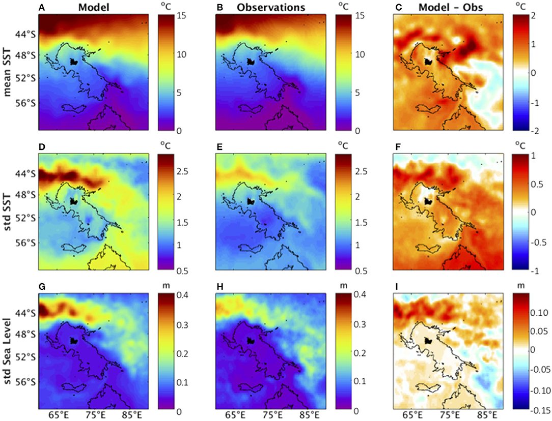
Figure 1. Mean SST (1994–2016) in (A) OFAM, (B) NOAA-OI observation-based product, and (C) the difference between model and observations; (D–F) same as in (A–C) but for SST standard deviation; (G–I) same as in (A–C) but for sea level standard deviation in (G) OFAM and (H) AVISO satellite altimetry.

FIGURE 2

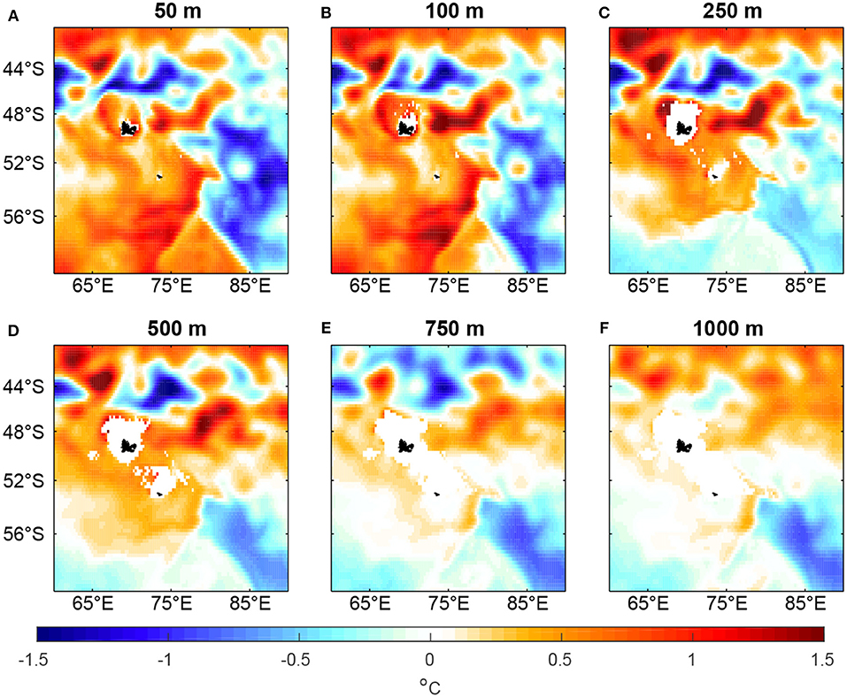
Figure 2. Temperature difference between OFAM and WOA2013 at (A) 50 m, (B) 100 m, (C) 250 m, (D) 500 m, (E) 750 m, and (F) 1,000 m.

The systematic biases in temperature mean and variability found in the model are removed in the MHW calculation, as the threshold that determines whether the ocean temperature is extreme or not is calculated for each dataset separately. In other words, the bias removal here is a consequence of how we calculate the MHWs, as the threshold to determine if the ocean has reached extreme temperatures is calculated separately for each dataset. For example, say that in a given part of the ocean, for 15th of January, the temperature's 90th percentile relative to climatology was 11°C based on observed data. However, if in the model simulation, the same place and corresponding date has a 90th percentile of 9°C, then the model simulation is seen to have a negative temperature bias at this point in space and time. Now, for example in a particular year, e.g., on the 15th of January 2014, the ocean was 12°C in the observations, and 10°C in the model. If we use the 11°C observation-based 90th percentile as a threshold for the model, that region would not have extreme ocean temperatures. However, if we use the 9°C model-based 90th percentile as a threshold, the region would have extreme temperatures. Therefore, even if the model has a negative bias, the fact that we calculate the 90th percentile separately using the model data, extreme temperature events can still correspond, despite the bias.

To validate OFAM at depth, we compare the modeled temperature to the World Ocean Atlas version 2 (WOA2013; Locarnini et al., 2018). WOA2013 is a set of objectively analyzed climatological fields, in a 1° grid, of several in situ ocean properties, including temperature. At depth, the modeled ocean temperature is also warmer than observations over and to the west of the plateau, with biases decreasing below 750 m (Figure 2). The largest biases of temperature at depth relate to the strong ACC flow to the north of the plateau. Despite local biases, the modeled regional circulation and variability are well-represented, both at the surface and at depth.

The mean frequency, duration, and intensity of MHWs in the KP region reflect the local ocean dynamics, both in the observations (Figures 3A–C) and in the model output (Figures 3D–F). To the north and east of the KP, the ACC influence is strong, and the high SST variability (Figures 1D,E) is associated with the presence of mesoscale eddies and meanders (van Wijk et al., 2010). The MHWs that happen at this location are more frequent (up to three events per year) and more intense (up to 4°C above climatology) than in other regions of the KP (Figures 3A,C). These MHWs to the north and east of the KP are associated with transient warm-core eddies that propagate eastwards, advected by the ACC.

FIGURE 3

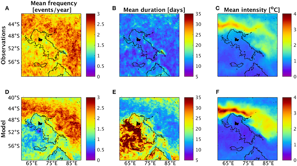
Figure 3. MHW mean (A) frequency, (B) duration, and (C) intensity in NOAA-OI gridded observation-based product (1994–2016); (D–F) as in (A–C), but for OFAM. The black line is the 3,000 m isobath.

To the south and west of the KP, the MHWs are less frequent than in the eastern side of the KP (Figures 3A,D). However, according to the model, these less frequent MHWs are longer-lasting, with a mean duration of longer than 35 days (Figure 3E). The long duration of MHWs at this location relates to the semi-stationarity of the flow in this portion of the KP (van Wijk et al., 2010). MHW frequency and duration are related metrics, as the more frequent the MHWs are, the shorter they tend to be, and vice-versa. This interplay between MHW frequency and duration is clear in the model output, where more frequent and shorter MHWs occur to the northeast of the KP, while less frequent and longer MHWs occur to the southwest of the KP (Figures 3D,E). In the observations, however, these patterns are not as clear, with MHWs lasting, on average, ~10 days across the whole domain (Figure 3B).

Globally, modeled MHWs have been described to be less frequent, longer-lasting, and weaker than observed MHWs (Pilo et al., 2019). To the north of the KP, in contrast to the results in Pilo et al. (2019), modeled MHWs are more intense than observed MHWs. To the west of the KP and on the plateau itself, however, results corroborate with those from the global analysis. The higher frequency of modeled MHWs might relate to the difference between the thickness of the model's surface level, and the thickness of the surface layer represented in observation-based products (Pilo et al., 2019). While OFAM's surface represents the top 2.5 m of the water column, the NOAA-OI product represents just the top 0.5 m of the ocean. Therefore, the NOAA-OI product is expected to be more varying, and have more numerous intermittent MHWs, than OFAM.

The overall pattern of MHW distribution and intensity are in agreement between the model and the observations (Figure 3). These results suggest that MHWs on the eastern KP are mainly driven by warm-core ocean eddies, while MHWs on the western KP are driven by less-transient, and possibly larger-scale, processes. The MHWs that occur over the KP (i.e., in waters shallower than 3,000 m) belong to the latter group. As characterizing MHWs over the KP is the key focus of this study, we further investigate the occurrence of the plateau-wide MHWs over the 23-years record.

In the observations, between January 1994 and December 2016, the SST on the KP exceeds its 90th percentile in the austral summers of 1997, 2003–2004, and 2009–2013 (Figure 4A, when the black line exceeds the green line). Amongst these events, the strongest and most persistent anomalous warming over the KP occurs between December 2011 and December 2012 (Figure 4B). This warming period peaks during the winter of 2012, with up to 2°C above climatology over the KP (Figure 4C). Because of high SST variability, this warming event is intermittent at a given location (i.e., 76°E, 53°S, magenta dot in Figure 4D). However, a map of cumulative SST anomaly (SSTA) between December 2011 and June 2013 indicates that the MHW extends over the whole KP (Figure 4D).

FIGURE 4

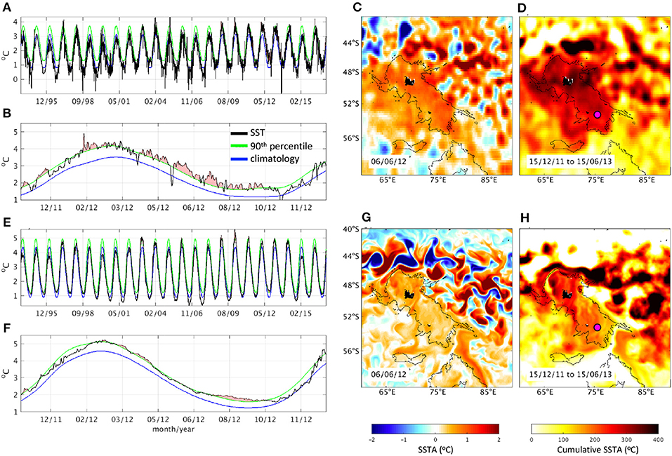
Figure 4. (A) Time-series of SST (black), climatology (blue) and 90th percentile (green) in NOAA-OI observation-based product for 1994–2016 in the magenta dot shown in (D); (B) as in (A) but for November 2011 to December 2012; (C) SSTA snapshot of July 2012 in NOAA-OI; and (D) cumulative SSTA of December 2011 to July 2013 in NOAA-OI; (E–H) as in (A–D), but for OFAM. Black contours are the 3,000 m isobath.

In the model output, the simulated SST exceeds its 90th percentile in the summers of 2003, 2006, and 2009–2013 (Figure 4E). The strongest events seen in the observations (Figure 4A), between 2009 and 2013, are well-represented in the model output. In addition, the strongest event seen in the observations (December 2011–December 2012) is also well-simulated (Figures 4F–H). The model simulates the anomalously warm SST over the winter of 2012, peaking in August 2012 (Figure 4F). The map of cumulative SSTA between December 2011 and June 2013 indicates that the simulated MHW also extends over the whole KP. The modeled MHW peaks to the east of the KP, but still covers the entire plateau and surrounding slopes limited by the 3,000 m isobath (Figure 4H).

Six of the seven summers under MHW conditions in the model output coincide with summers under MHW conditions identified in the observation-based product (Figures 4A,E). This result gives us confidence that the model is simulating the MHWs forced by local to regional-scale processes, such as changes in the wind patterns or changes in the air-ocean heat flux. In addition, both the persistence of the anomalous warming over the 2012 winter, and the spatial pattern of stronger SSTA, are simulated in the model output. Therefore, we use the model to investigate the penetration of the strong MHW event of 2012 from the ocean's surface to the ocean's subsurface.

The pattern of extremely hot temperatures over the KP region changes with depth and in time during 2012 (Figure 5A). Early in 2012, temperatures exceeding the 90th percentile threshold spread over the northern part of the KP at the surface level, but not at 100 m depths. At the surface, the extreme signature persists until September, dissipating in November. At 100 m depths, the extreme signature emerges in July, persisting until the end of the year. At 200 m depths, there is an extreme signature in the northern part of the KP that seems to be unrelated to the pattern seen at the surface. Later in the year, extreme hot anomalies spread over the whole KP. In a given location, the 2012 MHW is seen as temperature anomalies of up to 2°C above climatology, spreading from the surface to ~150 m depths (Figures 5B,C). Compared to other years, the positive anomaly values in 2012 were more persistent, more intense, and penetrated deeper. This positive anomaly in 2012 was even more persistent over the plateau (Figure 5C) than to the west of the plateau (Figure 5B).

FIGURE 5

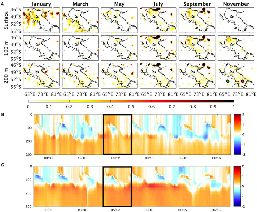
Figure 5. (A) Monthly average of extreme temperatures (i.e., above the 90th percentile relative to climatology) for alternated months of 2012 at the surface (top), 100 m (middle), and 200 m (bottom) depths in OFAM; (B) Temperature anomaly, relative to climatology, at the western green dot in the last panel of (A), from surface to 250 m depths; (C) as in (B), but for the eastern pink dot in the last panel of (A); the black box indicates the year 2012.

We show that, in 2012, the KP was under MHW conditions that persisted from summer through winter, with anomalously warm waters penetrating down to 150 m depths. Considering the large spatial and temporal distribution of the MHW, and its presence in both the observations and in the free-running model, we hypothesize that this anomalous event and its deepening in the water column are forced by a large scale atmospheric pattern. Next, we investigate the action of the wind field as a deepening mechanism for this strong MHW event.

In 2012, the wind stress curl (WSC) over the KP varies between 1.2 × 10⁻⁷ and −1.5 × 10⁻⁷ N/m³ (Figure 6A). The maximum WSC over the KP, which would result in downwelling, occurs in July (Figure 6B). The minimum WSC over the KP, associated with upwelling, occurs in October/November (Figure 6C). The values of WSC in these months are the minimum for the whole time period analyzed in this study. Comparing these results with Figure 5, the month with deepest penetration of anomalously warm waters, coincides with the month of strongest wind-driven downwelling (i.e., July 2012). Therefore, this wind-driven Ekman pumping could be responsible for the penetration and persistence of the 2012 MHW through the winter months. In November 2012, the WSC changes, with upwelling conditions becoming dominant over the KP. These upwelling conditions lead to the dissipation of the MHW at depth over the following months, as seen in the SST time-series in Figures 4B,C.

FIGURE 6

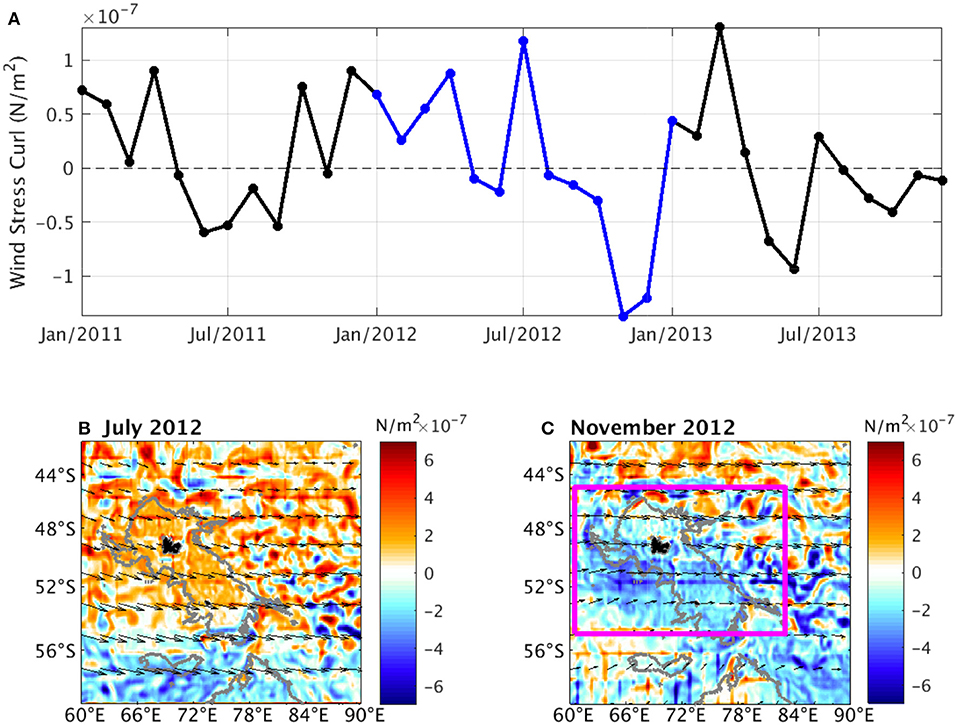
Figure 6. (A) Time-series of spatially averaged wind stress curl in the region delimited by the magenta box in (C), between January 2011 and December 2013. The blue line indicates the year 2012; (B,C) maps of wind stress curl (colors) and wind stress (arrows) in July 2012 and November 2012, respectively. The gray line is the 3,000 m isobath.

The wind conditions over the KP may also be modulated by remote large-scale forcing changes via atmospheric teleconnections. Thus, we now investigate the possible contribution from large-scale climate modes to the changes temperature over the plateau. For this analysis, we calculate the correlation between ocean temperature at the surface and at 150 m depths over the KP with the indices of four large-scale climate modes (Figure 7).

FIGURE 7

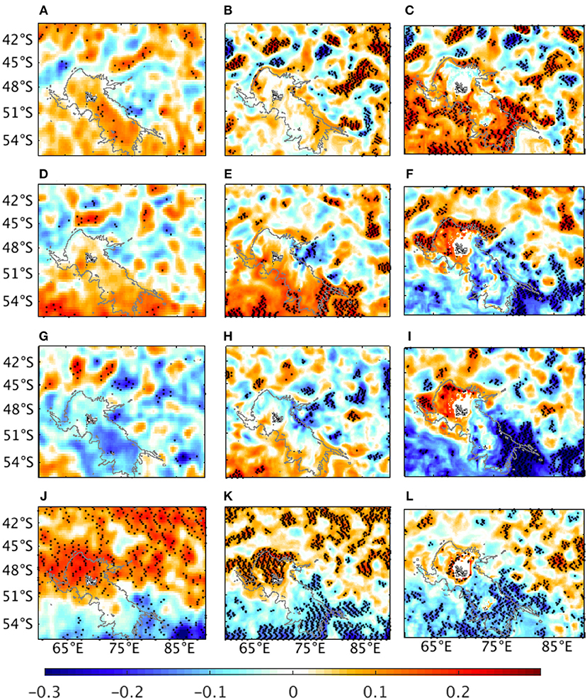
Figure 7. Maps of point-wise correlation coefficients between SST from NOAA-OI (left), temperature at the surface in OFAM (center), and temperature at 150 m in OFAM (right) and indices (single time series) of the following climate modes: (A–C) IOD, (D–F) ENSO, (G–I) PDO, and (J–L) SAM, between Jan 1994 and Dec 2016; the stippling (black dots) indicates regions where the correlations are statistically significant at the 95% confidence level, taking account of the effective number of degrees of freedom; the gray line indicates the 3,000 m isobath.

At the surface, in both model and observations, IOD, ENSO, and SAM are significantly correlated with ocean temperature over several portions the KP (Figures 7A–L). The highest correlation, as expected, happens between KP waters and the SAM, with clear patterns to the north and to the south of the KP (Figures 7J,K). SAM is the dominant mode of variability across the Southern Hemisphere mid to high latitudes. Nevertheless, ENSO has a significant positive correlation with surface waters to the south of the KP (Figures 7D,E). ENSO is the dominant global mode of interannual climate variability, albeit dynamically centered across the tropical Pacific atmosphere-ocean. The correlation between the IOD and surface temperatures differs between the model and the observations. In the observations, there is a positive correlation between this index and waters shallower than 3,000 m depths (Figure 7A), with some significant correlation evident in the center of the KP. However, in the model, significant values are only found to the north of the KP, associated with the ACC (Figure 7B). This latter pattern, and also the pattern of correlation between surface temperature and the PDO, are not coherent.

At 150 m depths, all investigated climate modes are significantly correlated with the ocean's temperature (Figures 7C,F,I,L). Correlations between ocean temperature and ENSO, PDO, SAM are similar at this depth, with positive values in the northern part of the plateau, and negative values in the southern part of the plateau (Figures 7F,I,L). There is also a significant correlation between the deep waters over almost the entire KP and the IOD (Figure 7A).

We show that the strong 2012 MHW event on the KP penetrates to a depth of 200 m during winter. This depth penetration is likely linked to the wind pattern found over the KP for those months, which favored downwelling. In November, when the MHW dissipates, the wind pattern favors upwelling. As we show here, Gille et al. (2014) also find that cold SSTs correlate with winds favoring upwelling over the KP. The effect of the regional wind circulation has been linked to the deepening of MHWs before, although in a study region that was coastal. Schaeffer and Roughan (2017) show that downwelling-favorable winds reduce the ocean stratification off eastern Australia, mixing the water column and aiding the deepening of anomalously hot SST. Downwelling-favorable winds have also been linked to the persistence of the 2013/2014 MHW along the North American west coast and its role in toxic algal blooms (McCabe et al., 2016). In addition to the wind-stress, other mechanisms may have played a role in the 2012 MHW deepening include ocean eddies, and Rossby waves. Specifically, stationary Rossby waves have been linked to strong vertical velocities over the KP, and to high anthropogenic carbon sequestration at this location as a result (Langlais et al., 2017).

The significant correlation between climate modes and SST over the KP suggests that MHWs in the region may also be influenced by remote oceanographic drivers. The influence of remote drivers manifests via either atmospheric or oceanic teleconnections, which can act to modulate the local circulation (Holbrook et al., 2019). Examples of atmospheric teleconnections here are atmospheric bridges or atmospheric Rossby waves, and an example of an oceanic teleconnection are oceanic Rossby waves. Climate modes are important remote MHW drivers in many regions of the ocean (Holbrook et al., 2019, and literature therein). In the broader KP region (i.e., 40–60°S, 50–90°E), the positive phase of the SAM, the negative phase of the Atlantic Niño index, and the positive phase of the Northern Atlantic Oscillation have been shown to be significantly related to increased MHW occurrence (Holbrook et al., 2019). It is relevant to note that Holbrook et al. (2019), however, only show the dominant climate modes in each oceanic region, and that the other modes identified in our results could well be the second or third significant modes at these locations. Here, we further show that the IOD is significantly correlated with waters over the plateau itself, while ENSO is correlated with waters to the south of the plateau, and SAM with waters to the north of the plateau. Despite this short duration, the 2012 IOD was intense, impacting tropical and subtropical ocean temperatures. Therefore, it is likely that the 2012 MHW in the KP region was influenced by this unusual IOD phase. The correlation between SST over the KP and climate modes suggests that there may be potential predictability for MHWs in this region. Furthermore, considering that the IOD is the dominant mode over the KP itself, it may be a reasonable metric for shallow water variability over the plateau.

4. Conclusions

We show that strong MHWs can occur in the KP region and that a significant MHW occurred in the region during 2012. More than that, MHWs over the KP can persist over winter months and can penetrate into the subsurface of the ocean. Many Southern Ocean species are dependent on the regular interannual temperature cycle that exists in this region and are likely to be impacted by the gradual long term change that is projected by anthropogenic climate change (Constable et al., 2014). It is also likely that many species will be impacted much sooner by ocean temperature extremes that occur during MHWs (e.g., Smale et al., 2019). In turn, as the climate warms, MHWs are projected to become more intense and occur more frequently (Oliver et al., 2018). As such, the characterization of MHWs in the KP region are key to understanding the environmental changes likely to be seen across a warming KP. The knowledge of environmental changes can then be used to investigate potential impacts on the populations of marine species (Goedegebuure et al., 2018). These investigations are especially important to understand the future population trajectories of threatened species which use the KP region for both food and as a breeding habitat, and for commercially exploited species that occur on the KP.

Data Availability Statement

The datasets analyzed in this study can be found in the Bluelink repository (http://dapds00.nci.org.au/thredds/catalog/gb6/OFAM3/catalog.html, downloaded in August 2019), in the AVISO webpage (https://www.aviso.altimetry.fr), and in the NOAA webpage (https://www.esrl.noaa.gov/psd/data/gridded/data.noaa.oisst.v2.highres.html).

Author Contributions

ZS and GP performed the analysis of this study. GP, SC, and NH wrote the paper. SC and NH conceptualized the study. MM and PZ provided support with the analysis and on interpretation of the results. All authors contributed to the article and approved the submitted version.

Funding

GP and NH received funding support from the Australian Research Council Centre of Excellence for Climate Extremes (CE170100023). MM received funding support from JSPS KAKENHI (JP19J01838). SC, NH, and PZ received funding support from the Fisheries Research and Development Corporation (FRDC 2018-133).

Conflict of Interest

The authors declare that the research was conducted in the absence of any commercial or financial relationships that could be construed as a potential conflict of interest.

Acknowledgments

The authors thank Dirk Welsford (Australian Antarctic Division) and Nicole Hill (Institute for Marine and Antarctic Studies) for providing advice and feedback and Bluelink, a partnership between CSIRO, the Bureau of Meteorology and the Royal Australian Navy, for developing and making available the model used in this study. This research was undertaken with the assistance of resources from the National Computational Infrastructure (NCI), which was supported by the Australian Government. Sea level products were processed by SSALTO/DUACS and distributed by AVISO+ with support from CNES. Some of the code used to perform this analysis was written and made publicly available by Z. Zhao and M. Marin (Zhao and Marin, 2019).

References

Bailleul, F., Cotté, C., and Guinet, C. (2010). Mesoscale eddies as foraging area of a deep-diving predator, the southern elephant seal. Mar. Ecol. Prog. Ser. 408, 251–264. doi: 10.3354/meps08560

CrossRef Full Text | Google Scholar

Blunden, J., and Arndt, D.S. (2017). State of the climate in 2016. Bull. Am. Meteorol. Soc. 98, S1–S280. doi: 10.1175/2017BAMSStateoftheClimate.1

CrossRef Full Text | Google Scholar

Boyd, P. W. (2002). Environmental factors controlling phytoplankton processes in the Southern Ocean. J. Phycol. 38, 844–861. doi: 10.1046/j.1529-8817.2002.t01-1-01203.x

CrossRef Full Text | Google Scholar

Bracegirdle, T. J., Hyder, P., and Holmes, C. R. (2018). CMIP5 diversity in southern westerly jet projections related to historical sea ice area: strong link to strengthening and weak link to shift. J. Clim. 31, 195–211. doi: 10.1175/JCLI-D-17-0320.1

CrossRef Full Text | Google Scholar

Cavagna, A. J., Fripiat, F., Elskens, M., Mangion, P., Chirurgien, L., Closset, I., et al. (2015). Production regime and associated N cycling in the vicinity of Kerguelen Island, Southern Ocean. Biogeosciences 12, 6515–6528. doi: 10.5194/bg-12-6515-2015

CrossRef Full Text | Google Scholar

Cavole, L., Demko, A., Diner, R., Giddings, A., Koester, I., Pagniello, C., et al. (2016). Biological impacts of the 2013–2015 warm-water anomaly in the northeast Pacific: winners, losers, and the future. Oceanography 29, 273–285. doi: 10.5670/oceanog.2016.32

CrossRef Full Text | Google Scholar

Collins, M., Knutti, R., Arblaster, J., Dufresne, J. L., Fichefet, T., Friedlingstein, P., et al. (2013). “Long-term climate change: projections, commitments and irreversibility,” in Climate Change 2013: The Physical Science Basis. Contribution of Working Group I to the Fifth Assessment Report of the Intergovernmental Panel on Climate Change (Cambridge; New York, NY: Cambridge University Press).

Google Scholar

Collins, M. A., Brickle, P., Brown, J., and Belchier, M. (2010). The Patagonian toothfish: biology, ecology and fishery. Adv. Mar. Biol. 58, 227–300. doi: 10.1016/B978-0-12-381015-1.00004-6

PubMed Abstract | CrossRef Full Text | Google Scholar

Constable, A. J., Melbourne-Thomas, J., Corney, S. P., Arrigo, K. R., Barbraud, C., Barnes, D. K. A., et al. (2014). Climate change and Southern Ocean ecosystems I: how changes in physical habitats directly affect marine biota. Glob. Change Biol. 20, 3004–3025. doi: 10.1111/gcb.12623

PubMed Abstract | CrossRef Full Text | Google Scholar

Darmaraki, S., Somot, S., Sevault, F., Nabat, P., Cabos Narvaez, W. D., Cavicchia, L., et al. (2019). Future evolution of marine heatwaves in the Mediterranean Sea. Clim. Dyn. 53, 1371–1392. doi: 10.1007/s00382-019-04661-z

CrossRef Full Text | Google Scholar

Davis, R. E. (1976). Predictability of sea surface temperature and sea level pressure anomalies over the North Pacific Ocean. J. Phys. Oceanogr. 6, 249–266.

Google Scholar

Dee, D. P., and Uppala, S. (2009). Variational bias correction of satellite radiance data in the ERA-Interim reanalysis. Q. J. R. Meteorol. Soc. 135, 1830–1841. doi: 10.1002/qj.493

CrossRef Full Text | Google Scholar

Dragon, A. C., Monestiez, P., Bar-Hen, A., and Guinet, C. (2010). Linking foraging behaviour to physical oceanographic structures: Southern elephant seals and mesoscale eddies east of Kerguelen Islands. Prog. Oceanogr. 87, 61–71. doi: 10.1016/j.pocean.2010.09.025

CrossRef Full Text | Google Scholar

Duhamel, G., Pruvost, P., Bertignac, M., Gasco, N., and Hautecoeur, M. (2011). “Major fishery events in Kerguelen Islands: Notothenia rossi, Champsocephalus gunnari, Dissostichus eleginoides–current distribution and status of stocks,” in The Kerguelen Plateau: Marine Ecosystem and Fisheries, eds D. Duhamel and D. C. Welsford (Paris: Société Française d'Ichtyologie), 258–286.

Google Scholar

Frölicher, T. L., and Laufkötter, C. (2018). Emerging risks from marine heat waves. Nat. Commun. 9, 2015–2018. doi: 10.1038/s41467-018-03163-6

PubMed Abstract | CrossRef Full Text | Google Scholar

Fyfe, J. A., Saenko, O. A., Zickfeld, K., Eby, M., and Weaver, A. J. (2007). The role of poleward-intensifying winds on Southern Ocean warming. J. Clim. 20, 5391–5400. doi: 10.1175/2007JCLI1764.1

CrossRef Full Text | Google Scholar

Garrabou, J., Coma, R., Bensoussan, N., Bally, M., Chevaldonné, P., Cigliano, M., et al. (2009). Mass mortality in Northwestern Mediterranean rocky benthic communities: effects of the 2003 heat wave. Glob. Change Biol. 15, 1090–1103. doi: 10.1111/j.1365-2486.2008.01823.x

CrossRef Full Text | Google Scholar

Gille, S. T. (2002). Warming of the Southern Ocean since the 1950's. Science 295, 1275–1277. doi: 10.1126/science.1065863

CrossRef Full Text | Google Scholar

Gille, S. T., Carranza, M. M., Cambra, R., and Morrow, R. (2014). Wind-induced upwelling in the Kerguelen Plateau region. Biogeosciences 11, 6389–6400. doi: 10.5194/bg-11-6389-2014

CrossRef Full Text | Google Scholar

Goedegebuure, M., Melbourne-Thomas, J., Corney, S. P., McMahon, C. R., and Hindell, M. A. (2018). Modelling southern elephant seals Mirounga leonina using an individual-based model coupled with a dynamic energy budget PLoS ONE 13:e0194950. doi: 10.1371/journal.pone.019495

PubMed Abstract | CrossRef Full Text | Google Scholar

Haumann, A. F., Gruber, N., and Matthias, M. (2020). Sea-ice induced Southern Ocean subsurface warming and surface cooling in a warming climate. AGU Adv. 1:e2019AV000132. doi: 10.1029/2019AV000132

CrossRef Full Text | Google Scholar

Hill, N. A., Foster, S. D., Duhamel, G., Welsford, D., Koubbi, P., and Johnson, C. R. (2017). Model-based mapping of assemblages for ecology and conservation management: a case study of demersal fish on the Kerguelen Plateau. Divers. Distrib. 23, 1216–1230. doi: 10.1111/ddi.12613

CrossRef Full Text | Google Scholar

Hindell, M. A., Lea, M., Bost, C., Charassin, J. B., Gales, N., Goldsworthy, S., et al. (2011). “Foraging habitats of top predators, and areas of ecological significance, on the Kerguelen Plateau,” in The Kerguelen Plateau: Marine Ecosystem and Fisheries, eds G. Duhamel and D. C. Welsford (Paris: Société Française d'Ichtyologie), 203–215.

Google Scholar

Hobday, A. J., Alexander, L. V., Perkins, S. E., Smale, D. A., Straub, S. C., Oliver, E. C. J., et al. (2016). A hierarchical approach to defining marine heatwaves. Prog. Oceanogr. 141, 227–238. doi: 10.1016/j.pocean.2015.12.014

CrossRef Full Text | Google Scholar

Holbrook, N. J., Scannell, H. A., Sen Gupta, A., Benthuysen, J., Feng, M., Oliver, E. C., et al. (2019). A global assessment of marine heatwaves and their drivers. Nat. Commun. 10:2624. doi: 10.1038/s41467-019-10206-z

PubMed Abstract | CrossRef Full Text | Google Scholar

Jackson, J. M., Johnson, G. C., Dosser, H. V., and Ross, T. (2018). Warming from recent marine heatwave lingers in deep British Columbia fjord. Geophys. Res. Lett. 45, 9757–9764. doi: 10.1029/2018GL078971

CrossRef Full Text | Google Scholar

Langlais, C. E., Lenton, A., Matear, R., Monselesan, D., Legresy, B., Cougnon, E., et al. (2017). Stationary Rossby waves dominate subduction of anthropogenic carbon in the Southern Ocean. Sci. Rep. 7:17076. doi: 10.1038/s41598-017-17292-3

PubMed Abstract | CrossRef Full Text | Google Scholar

Locarnini, R. A., Mishonov, A. V., Antonov, J. I., Boyer, T. P., Garcia, H. E., Baranova, O. K., et al. (2018). World Ocean Atlas 2018, Volume 1: Temperature. NOAA Atlas NESDIS 81, 52. Available online at: https://archimer.ifremer.fr/doc/00651/76338/

Google Scholar

Manta, G., de Mello, S., Trinchin, R., Badagian, J., and Barreiro, M. (2018). The 2017 record marine heatwave in the southwestern Atlantic shelf. Geophys. Res. Lett. 45, 12449–12456. doi: 10.1029/2018GL081070

CrossRef Full Text | Google Scholar

Matear, R. J., Chamberlain, M. A., Sun, C., and Feng, M. (2013). Climate change projection of the Tasman Sea from an Eddy-resolving ocean model. J. Geophys. Res. Ocean. 118, 2961–2976. doi: 10.1002/jgrc.20202

CrossRef Full Text | Google Scholar

McCabe, R. M., Hickey, B. M., Kudela, R. M., Lefebvre, K. A., Adams, N. G., Bill, B. D., et al. (2016). An unprecedented coastwide toxic algal bloom linked to anomalous ocean conditions. Geophys. Res. Lett. 43, 10366–10376. doi: 10.1002/2016GL070023

PubMed Abstract | CrossRef Full Text | Google Scholar

Meredith, M., Sommerkorn, M., Cassotta, S., Derksen, C., Ekaykin, A., Hollowed, A., et al. (2020). “2019: polar regions,” in IPCC Special Report on the Ocean and Cryosphere in a Changing Climate, eds H.-O. Pörtner, D. C. Roberts, V. Masson-Delmotte, P. Zhai, M. Tignor, E. Poloczanska, K. Mintenbeck, A. Alegría, M. Nicolai, A. Okem, J. Petzold, B. Rama, and N. M. Weyer (In press).

Google Scholar

Mills, K. E., Pershing, A. J., Brown, C. J., Chen, Y., Chiang, F. S., Holland, D. S., et al. (2013). Fisheries management in a changing climate. Oceanography 26, 191–195. doi: 10.5670/oceanog.2013.27

CrossRef Full Text | Google Scholar

Mueter, F. J., Peterman, R. M., and Pyper, B. J. (2002). Opposite effects of ocean temperature on survival rates of 120 stocks of Pacific salmon (Oncorhynchus spp.) in northern and southern areas. Can. J. Fish. Aquat. Sci. 59, 456–463. doi: 10.1139/f02-020

CrossRef Full Text | Google Scholar

Oke, P. R., Griffin, D. A., Schiller, A., Matear, R. J., Fiedler, R., Mansbridge, J., et al. (2013). Evaluation of a near-global eddy-resolving ocean model. Geosci. Model Dev. 6, 591–615. doi: 10.5194/gmd-6-591-2013

CrossRef Full Text | Google Scholar

Oliver, E. C., Benthuysen, J. A., Bindoff, N. L., Hobday, A. J., Holbrook, N. J., Mundy, C. N., et al. (2017). The unprecedented 2015/16 Tasman Sea marine heatwave. Nat. Commun. 8, 1–12. doi: 10.1038/ncomms16101

PubMed Abstract | CrossRef Full Text | Google Scholar

Oliver, E. C. J. (2019). Mean warming not variability drives marine heatwave trends. Clim. Dyn. 53, 1653–1659. doi: 10.1007/s00382-019-04707-2

CrossRef Full Text | Google Scholar

Oliver, E. C. J., Donat, M. G., Burrows, M. T., Moore, P. J., Smale, D. A., Alexander, L. V., et al. (2018). Longer and more frequent marine heatwaves over the past century. Nat. Commun. 9:1324. doi: 10.1038/s41467-018-03732-9

PubMed Abstract | CrossRef Full Text | Google Scholar

Oliver, E. C. J., and Holbrook, N. J. (2014). Extending our understanding of South Pacific gyre ‘spin-up': Modelling the East Australian Current in a future climate. J. Geophys. Res. Ocean. 119, 2788–2805. doi: 10.1002/2013JC009591

CrossRef Full Text | Google Scholar

Pilo, G. S., Holbrook, N. J., Kiss, A. E., and Hogg, A. M. (2019). Sensitivity of marine heatwave metrics to ocean model resolution. Geophys. Res. Lett. 46, 14604–14612. doi: 10.1029/2019GL084928

CrossRef Full Text | Google Scholar

Pilo, G. S., Oke, P. R., Coleman, R., Rykova, T., and Ridgway, K. (2018). Patterns of vertical velocity induced by Eddy distortion in an ocean model. J. Geophys. Res. Ocean. 123, 2274–2292. doi: 10.1002/2017JC013298

CrossRef Full Text | Google Scholar

Pilo, G. S., Oke, P. R., Rykova, T., Coleman, R., and Ridgway, K. (2015). Do east Australian current anticyclonic eddies leave the Tasman Sea? J. Geophys. Res. Ocean. 120, 8099–8114. doi: 10.1002/2015JC011026

CrossRef Full Text | Google Scholar

Quéguiner, B., Blain, S., and Trull, T (2011). “High primary production and vertical export of carbon over the Kerguelen Plateau as a consequence of natural iron fertilization in a high-nutrient, low-chlorophyll environment,” in The Kerguelen Plateau: Marine Ecosystem and Fisheries, eds G. Duhamel and D. C. Welsford (Paris: Société Française d'Ichtyologie), 169–174.

Google Scholar

Raymond, B., Lea, M. A., Patterson, T., Andrews-Goff, V., Sharples, R., Charrassin, J. B., et al. (2015). Important marine habitat off east Antarctica revealed by two decades of multi-species predator tracking. Ecography 38, 121–129. doi: 10.1111/ecog.01021

CrossRef Full Text | Google Scholar

Reynolds, R. W., Smith, T. M., Liu, C., Chelton, D. B., Casey, K. S., and Schlax, M. G. (2007). Daily high-resolution-blended analyses for sea surface temperature. J. Clim. 20, 5473–5496. doi: 10.1175/2007JCLI1824.1

CrossRef Full Text | Google Scholar

Rhein, M., Rintoul, S. R., Aoki, S., Campos, E., Chambers, R. A., Feely, R. A., et al. (2013). “Observations: ocean,” in Climate Change 2013: The Physical Science Basis. Contribution of Working Group I to the Fifth Assessment Report of the Intergovernmental Panel on Climate Change (Cambridge; New York, NY: Cambridge University Press).

PubMed Abstract | Google Scholar

Ridgway, K. R., and Dunn, J. R. (2003). Mesoscale structure of the mean east Australian current system and its relationship with topography. Prog. Oceanogr. 56, 189–222. doi: 10.1016/S0079-6611(03)00004-1

CrossRef Full Text | Google Scholar

Ridgway, K. R., and Godfrey, J. S. (2015). The source of the Leeuwin current seasonality. J. Geophys. Res. Ocean. 120, 6843–6864. doi: 10.1002/2015JC011049

CrossRef Full Text | Google Scholar

Roquet, F., Boehme, L., Block, B., Charrassin, J.-B., Costa, D., Guinet, C., et al. (2017). Ocean observations using tagged animals. Oceanography 30:139. doi: 10.5670/oceanog.2017.235

CrossRef Full Text | Google Scholar

Rykova, T., and Oke, P. R. (2015). Recent freshening of the east Australian current and its Eddies. Geophys. Res. Lett. 42, 9369–9378. doi: 10.1002/2015GL066050

CrossRef Full Text | Google Scholar

Rykova, T., Oke, P. R., and Griffin, D. A. (2017). A comparison of the structure, properties, and water mass composition of quasi-isotropic Eddies in western boundary currents in an Eddy-resolving ocean model. Ocean Model. 114, 1–13. doi: 10.1016/j.ocemod.2017.03.013

CrossRef Full Text | Google Scholar

Scannell, H. A., Pershing, A. J., Alexander, M. A., Thomas, A. C., and Mills, K. E. (2016). Frequency of marine heatwaves in the North Atlantic and North Pacific since 1950. Geophys. Res. Lett. 43, 2069–2076. doi: 10.1002/2015GL067308

CrossRef Full Text | Google Scholar

Schaeffer, A., and Roughan, M. (2017). Subsurface intensification of marine heatwaves off southeastern Australia: the role of stratification and local winds. Geophys. Res. Lett. 44, 5025–5033. doi: 10.1002/2017GL073714

CrossRef Full Text | Google Scholar

Schiller, A., and Oke, P. R. (2015). Dynamics of ocean surface mixed layer variability in the Indian Ocean. J. Geophys. Res. Ocean. 120, 4162–4186. doi: 10.1002/2014JC010538

CrossRef Full Text | Google Scholar

Smale, D. A., Wernberg, T., Oliver, E. C., Thomsen, M., Harvey, B. P., Straub, S. C., et al. (2019). Marine heatwaves threaten global biodiversity and the provision of ecosystem services. Nat. Clim. Change 9, 306–312. doi: 10.1038/s41558-019-0412-1

CrossRef Full Text | Google Scholar

van Wijk, E. M., Rintoul, S. R., Ronai, B. M., and Williams, G. D. (2010). Regional circulation around Heard and McDonald Islands and through the Fawn Trough, central Kerguelen Plateau. Deep. Res. I Oceanogr. Res. Pap. 57, 653–669. doi: 10.1016/j.dsr.2010.03.001

CrossRef Full Text | Google Scholar

Wernberg, T., Bennett, S., Babcock, R. C., de Bettignies, T., Cure, K., Depczynski, M., et al. (2016). Climate-driven regime shift of a temperate marine ecosystem. Science 353, 169–172. doi: 10.1126/science.aad8745

PubMed Abstract | CrossRef Full Text | Google Scholar

Wernberg, T., Smale, D. A., Tuya, F., Thomsen, M. S., Langlois, T. J., De Bettignies, T., et al. (2013). An extreme climatic event alters marine ecosystem structure in a global biodiversity hotspot. Nat. Clim. Change 3, 78–82. doi: 10.1038/nclimate1627

CrossRef Full Text | Google Scholar

Zhao, Z., and Marin, M. (2019). A MATLAB toolbox to detect and analyze marine heatwaves. J. Open Source Softw. 4:1124. doi: 10.21105/joss.01124

CrossRef Full Text | Google Scholar

Zisserson, B., and Cook, A. (2017). Impact of bottom water temperature change on the southernmost snow crab fishery in the Atlantic Ocean. Fish. Res. 195, 12–18. doi: 10.1016/j.fishres.2017.06.009

CrossRef Full Text | Google Scholar