That’s All I Know: Inferring the Status of Extremely Data-Limited Stocks

Introduction

Depending on the amount of available information, fish stocks can be characterized as data-rich or data-limited. Data-rich stocks contain enough information to carry out analytical stock assessments, while data-limited ones do not. However, there are several levels of data-limitation. The International Council for the Exploration of the Sea (ICES) identifies six different stock categories with regards to data availability (ICES, 2012). Categories 1 and 2 include data-rich stocks with age-structured catch and survey data allowing quantitative assessments. These assessments are considered to describe adequately the true trends of stock size and exploitation levels; as such, trends of category 1 and 2 stocks are used to monitor the effectiveness of fisheries regulations (STECF, 2020). Categories 3–6 include stocks with progressively increasing data limitations. In category 3, survey data are available which can indicate trends of mortality rates, recruitment, and biomass. In category 4, a time-series of catch data is available which allows an approximation of maximum sustainable yield (MSY). In category 5, only landings data are available. Finally, category 6 includes negligible landings stocks and stocks caught as bycatch. This latter category of extremely data-limited stocks is the focus of the current study.

There is an ever-growing number of data-limited assessment methods focusing on stocks falling primarily within data categories 3 to 5. For example, for category 3 stocks, the survey-based assessment method (SURBA) (Beare et al., 2005) or the time-series analysis assessment (TSA) (Fryer et al., 1998; ICES, 2008) can be used to estimate population numbers and fishing mortality rates based on survey data. For category 3/4 stocks, surplus production models can be used to estimate biomass and exploitation level for commercial stocks when their age and size data is absent (Punt, 2003). These models are suitable for stocks with data from commercial catches along with indices of exploitable biomass (from catch-per-unit-effort, or survey data) (Polacheck et al., 1993). For example, Pedersen and Berg (2017) presented a stochastic surplus production model in continuous time (SPiCT) which combines dynamics of biomass and fisheries with remarked error of catches and biomass indices. For category 4/5 stocks, where only time-series of catches or landings are available, methods such as the CMSY have been proposed (Martell and Froese, 2013) to estimate extracted yields in relation to MSY. Froese et al. (2017) updated the CMSY method by using catch and productivity to assess biomass. In addition, this method can approximate exploitation rate, MSY and fishing reference points. Froese et al. (2017) also used a Bayesian state-space estimation model (BSM) (Meyer and Millar, 1999) to verify and evaluate the CMSY model.

The examples of data-limited methods mentioned earlier are not exhaustive, but they are indicative of the fact that most data-limited methods require at least some information from surveys, commercial catches and productivity in order to estimate stock status. However, in the case of extremely data-poor stocks (category 6), it is not possible to apply such methods. In such cases, the starting point is the estimation of life history traits, such as growth and maturity. These life history traits can be used order to infer sustainable harvesting strategies, even if the exact stock status is unknown (Froese, 2004; Froese et al., 2008; Prince and Hordyk, 2019). Growth parameter estimates can also be used to estimate mortality rates, approximate reference points, and infer the stock status; a suite of different methods exists for every step of this way (Gayanilo and Pauly, 1997). Recently, a new method for the analysis of extremely data-limited stocks of fish and invertebrate species was proposed: the Length-based Bayesian Biomass (LBB) method (Froese et al., 2018). LBB requires only length frequency distributions (LFDs) as an input, as it makes a series of assumptions for the estimation of the missing life history information. LBB’s key outputs are the current exploited biomass relative to unexploited biomass (B/B0) and the fishing mortality relative to natural mortality (F/M) (Froese et al., 2018).

Typically, in extremely data-poor situations it is difficult to identify a single method that produces the ‘best’ estimate of a given variable. In that case, an ensemble modeling approach combining the outputs from multiple methods can help produce more robust estimates (Dormann et al., 2018). This process can in turn inform fisheries management more effectively and facilitate measures to promote fisheries sustainability.

In this study, we present a stepwise methodological framework to estimate the stock status of extremely data-limited stocks. We illustrate the use of this framework by estimating the stock status of an extremely data-limited shrimp stock (Plesionika edwardsii, Decapoda, Pandalidae), which is a bycatch of a small-scale trap fishery in the eastern Mediterranean Sea. Our proposed framework includes various methods for estimating growth parameters, calculating mortality rates, approximating reference points and eventually characterizing stock status. We synthesize the outputs from different model combinations, illustrating the advantages from using an ensemble modeling approach, and compare our findings with the outputs from a relevant LBB. This way, we elucidate the stock status of the studied shrimp stock and deduce implications for its management, in a way that is reproducible to other extremely data-limited stocks.

Materials and Methods

Sampling

Samples were collected in the Dodecanese archipelago (southeastern Aegean Sea) (Figure 1) from October 2014 to October 2015 on a monthly basis (except of February 2015 due to adverse weather conditions), under the framework of PLESIONIKA MANAGE project. PLESIONIKA MANAGE studied the biology and exploitation of Plesionika narval, a valuable fishery resource in the area (Kalogirou et al., 2017; Maravelias et al., 2018; Vasilakopoulos et al., 2019). P. edwardsii was a commercial bycatch of the fishery for P. narval, far less valuable than the targeted congeneric species.

FIGURE 1

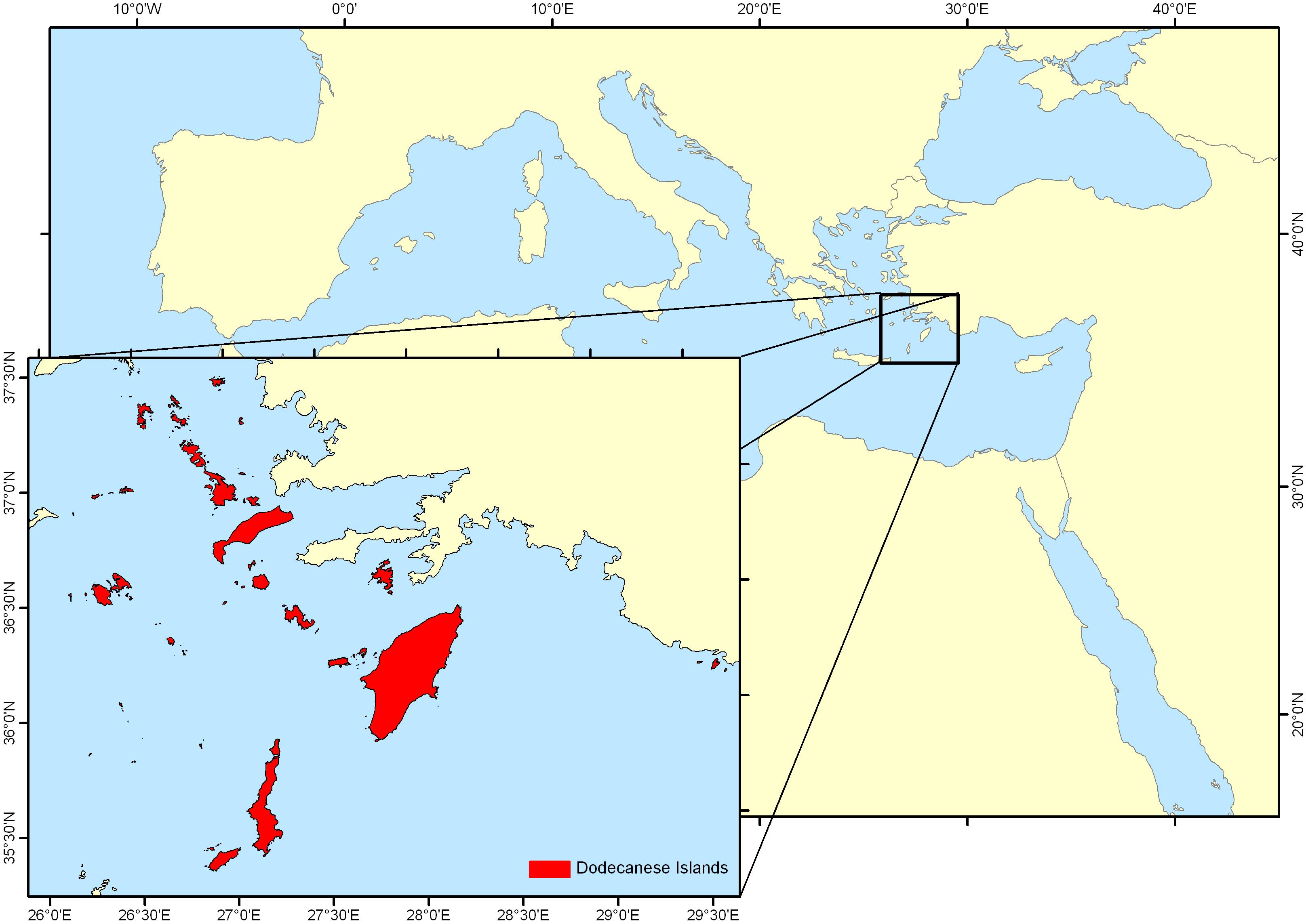
Figure 1. Map of sampling area – Dodecanese Islands, southeastern Aegean Sea, eastern Mediterranean Sea.

Sampling depth ranged from 0 to 280 m and was divided in strata A (0–45 m; depth of thermocline in the summer), B (46–100 m; to the end of the continental shelf), C (>100 m). Circular traps covered with nylon-based net of a mesh size of 12 mm (knot to knot) and with an upper trap opening of 13 cm were used (Kalogirou et al., 2019). Fishing took place during night hours (20:30- 06:00); after 9.5 h all traps were hauled, and the catch was separated in two categories: target (P. narval) and by-catch species, the latter including P. edwardsii. A random sample of approximately 100 shrimps, mainly P. narval, was collected from each stratum. The number, size (carapace length and body weight), sex and maturity stage of P. edwardsii shrimps within these samples was also documented (Figure 2).

FIGURE 2

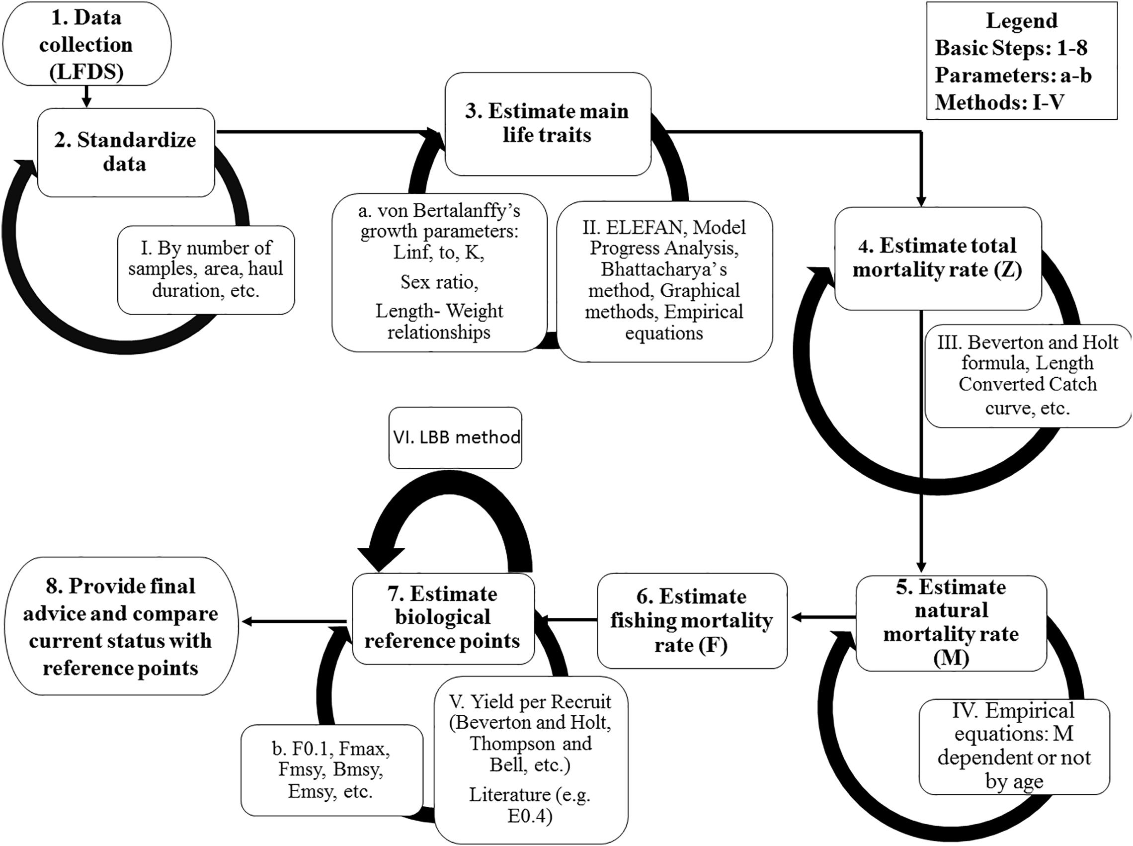
Figure 2. The basic steps (1–8) to assess an extremely data-limited stock, with a selection of associated methods.

Exploring and Processing Data

Carapace length (CL) was rounded at the nearest millimeter and LFDs were estimated by sex, maturation stage, month and depth strata, using length classes of 1 mm Due to the great variability of the sample size across months, standardized LFDs by month were estimated, by dividing the numbers of individuals within each length class by the total number of monthly samples (Figure 2). These standardized LFDs were used to:

(1) identify the main spawning periods;

(2) identify the depth distribution of males and females;

(3) estimate the sex ratio within each length class;

(4) create a length frequency object (LFQ) to be used for the estimation of the growth parameters. For this, the sex-combined LFD by month was restructured as a list object containing a catch frequency matrix, a vector of mid-lengths corresponding to rows of the catch matrix and a vector of sample dates corresponding to the columns of the catch matrix.

Estimation of Growth Parameters

This analysis was conducted using R programming language (R Core Team, 2020) and the TropFish R package (Mildenberger et al., 2017; Taylor and Mildenberger, 2017). To estimate growth parameters (Figure 2), the ELEFAN (Electronic Length Frequencies Analysis) program (available as tool in the TropFishR package) was used. ELEFAN calculates a moving average (MA) over the LFDs bin, and then compares the observed frequency with this average; values much above the average indicate a “true” mode (Pauly and David, 1981; Pauly, 1985). The LFQ file was prepared for running the ELEFAN by posing a MA to generate the Von Bertalanffy Growth Function (hereafter VBGF) estimations. For this, we set ranges for the infinite length (L_inf) and growth coefficient (K) values, and a theoretical time zero (t₀) at which individuals of this species hatch.

Preliminary estimations of L_inf were done based on three different approaches:

• the Powell and Wetherall method (Powell, 1979; Wetherall et al., 1987): a linearizing transformation of length classes to estimate L_inf by plotting L_mean – L’ and L’. L_mean is the mean length of all individuals greater than L’ and L’ is the smallest length of fully represented individuals in catches.

• the empirical formula from Froese and Binohlan (2000):L_inf=e^{0.44 + 0.984log(Lmax)}? with L_inf being infinite length and L_max being maximum observed length.

• the maximum carapace length observed in the samples.

The Powell and Wetherall method is very sensitive to intra-cohort variability in growth and to changes in the occurrence of large individuals in the sample, resulting often in underestimation of the L_inf value (Schwamborn, 2018). Exclusion of the largest size classes during the regression procedure or weighing by abundance does not resolve these issues (Schwamborn, 2018). By contrast, the Froese and Binohlan formula tends to overestimate L_inf values. Accordingly, two different length ranges for L_inf were chosen to run ELEFAN. The first length range had a lower limit of L_inf derived from the Powell and Wetherall method and the second one had a lower limit of L_inf equal to the maximum length observed in the samples. The L_inf value derived by the Froese and Binohlan formula was chosen as the upper limit for the length range of L_inf in both cases.

The range of K values was set between 0.4 to 0.9 y^–1, based on previous publications on the growth of this species (Santana et al., 1997; Company and Sardà, 2000; García-Rodriguez et al., 2000; Colloca, 2002).

Four different scenarios of the month when length is equal to zero (t_anchor in ELEFAN, conceptually similar to t₀ of the VBGF) were explored: (i) February, (ii) May, (iii) August, and (iv) November. The one resulting in the best fit and agreeing with the spawning information was chosen as the optimal t₀ (Supplementary Figures 6, 7).

The MA value used in the ELEFAN analysis was set based on two different scenarios. The first scenario used the default setting in FISAT II (Gayanilo and Pauly, 1997), i.e., a width of 5 bins (1 bin = 1 mm) for each cohort. Indeed, the smallest cohort width was up to 5 bins so it was plausible to compare each bin with the average across 5 consecutive bins (i.e., ±2 bins to either side). However, taking into consideration that the MA settings can significantly affect the scoring of the growth curve (Taylor and Mildenberger, 2017) a second scenario was also tested, with a 7-bin cohort width.

The estimation of the best fit was based on searching for the VBGF parameters with the maximum score value (Rn) as a measure of relative fit:

$$Rn=\frac{{10}^{ESP/ASP}}{10}$$

where the Estimated Sum of Peaks (ESP) is the sum of peak values crossed by the growth curves, with the caveat that positively crossed bins are only counted once, while negatively crossed bins are counted every time they are encountered (Pauly, 1985). The Available Sum of Peaks (ASP) is the sum of all positive peaks, which represents a maximum possible score (if negative bins are crossed). Rn can attain a maximum value of 1.

Fitting scores across the whole range of L_inf and K combinations was visualized by a Response Surface Analysis (RSA).

Estimating Total, Natural and Fishing Mortality

The VBGF parameters were used both to compute the length at which 50% of the cumulative catch is captured (L₅₀) and to estimate the total mortality (Z) (Figure 2) Z was computed using two methods:

• the Length Converted Catch Curve (LCCC) (Pauly, 1990)

• the relevant B&H formula (Beverton and Holt, 1956)

The Length Converted Catch Curve (Pauly, 1990) is a way to estimate Z plotting the natural logarithm (loge) of the number of fishes in the sample (N) against the relative age corresponding to the midrange of the length class in question [Δt is the time needed to grow from the lower (t₁) to the upper (t₂) limit of a given length class]:

$$lo{g}_{\text{e}}\left(\frac{N}{\mathrm{\Delta }}\right)=\mathrm{\alpha }-Zt$$

where a and Z are the regression parameters.

In the second case (Beverton and Holt, 1956), Z value is calculated as:

$$Z=\frac{K(L_{inf}-L_{mean})}{L_{mean}-L^{\prime }}$$

where L_inf and K are parameters from VBGF, L_mean is the mean length in the catches and L’ is the smallest length of animals that are fully represented in the catch samples.

A suite of different methods and formulas were used to estimate natural mortality (M) values (Figure 2 and Supplementary Table 1). This great number of methods reflects the fact that M is notoriously difficult to estimate (Kenchington, 2014), and it has a big effect on our perception of stock status (Mannini et al., in review). Four methods (and their variants) provided empirical scalar values (Alverson and Carney, 1975; Pauly, 1980; Hoenig, 1983; Hewitt and Hoenig, 2005; Then et al., 2014). Pauly’s (1980) equation was computed using three different bottom temperature values (14, 16, 18°C), based on the seasonal difference in bottom temperature. Seven more methods (and their variants) produced natural mortality vectors by age (Gulland, 1965; Chen and Watanabe, 1989; Caddy, 1991; Abella et al., 1997; Lorenzen, 2000; Gislason et al., 2010; Brodziak et al., 2011; Martiradonna, 2012) (Supplementary Figure 10). The estimated VBGF parameters were used to convert the maximum CL observed in the catch into age. For each of the M vectors by age a mean over the range between age 0 and maximum observed age was computed to obtain the corresponding scalar value.

This process resulted in sixteen different M scalar values. These values were subtracted from the two Z values calculated earlier, to provide a set of 32 different values of fishing mortality (F) (Figure 2).

Reference Points and Advice

In the final stage of the analysis, reference points for management (Caddy and Mahon, 1995) were computed according to a Yield per Recruit (YpR) model (Beverton and Holt, 1957) (Figure 2). In the Mediterranean, two reference points are being used for exploitation levels: F_0.1 and E_0.4 (STECF (17-15), 2017; STECF (19-16), 2019). The fishing mortality level F_0.1 is the F rate at which the slope of the yield per recruit curve as a function of F is 10% of its value at the origin (Gulland and Boerema, 1973). E_0.4 comes from Patterson (1992) who suggested as reference point in terms of exploitation rate (E), in particular for pelagic stocks, a value of_} E = F/Z = 0.4.

Thirty two different YpR analyses were run, corresponding to the 32 estimates of F, to extract the respective F_0.1 values. For all scenarios, L₅₀ of the selectivity was set as the length of 50% of the cumulative catch. The status of exploitation was estimated according to two ratios: $\frac{F}{F0.1}$ and $\frac{E}{E0.4}$, for which values over 1 indicate overfishing.

A kobeplot was used to visualize the 32 scenarios results (statuses of exploitation), as well as the mean and the median of them (Figure 2). Four areas with different colors based of E status were plotted in a Cartesian system in which x-y intersection is set at point equal to 1, 1. In the green area fell points having ratios below or equal to 1 for both $\frac{E}{E0.4}$ and$\frac{F}{F0.1}$. In the red area fell points having both ratios over 1 and, in the yellow areas points for which one of the two ratios was over 1.

Applying the LBB Method

LBB (Froese et al., 2018) requires only LFDs and is able to estimate L_inf, length at first capture, relative natural mortality (M/K) and relative fishing mortality (F/K). M/K and F/K can be combined to give fishing mortality relative to natural mortality (F/M). LBB also estimates an approximation of current exploited biomass relative to unexploited biomass (B/B₀).

To apply this method, the monthly LFDs we had available were aggregated to a yearly sample. The L_inf prior was set equal to our best estimation from ELEFAN. In assigning M/K priors, K was set equal to our best estimation from ELEFAN while M values changed according to the 16 methods presented in chapter “Estimating total, natural and fishing mortality.” All other inputs were set to the default values suggested by Froese et al. (2018).

Results

Length Frequency Distributions

In total, 1993 P. edwardsii individuals were sampled. Plotting the LFD using the raw data showed strong monthly variability in the number of individuals (unbalanced data), ranging from 4 in October 2014 to 693 in November 2014, and irregular population distributions (Tables 1, 2). The length at which 50% of the cumulative catch is captured (L₅₀) was estimated as 21.70 mm. (Supplementary Figure 8).

TABLE 1

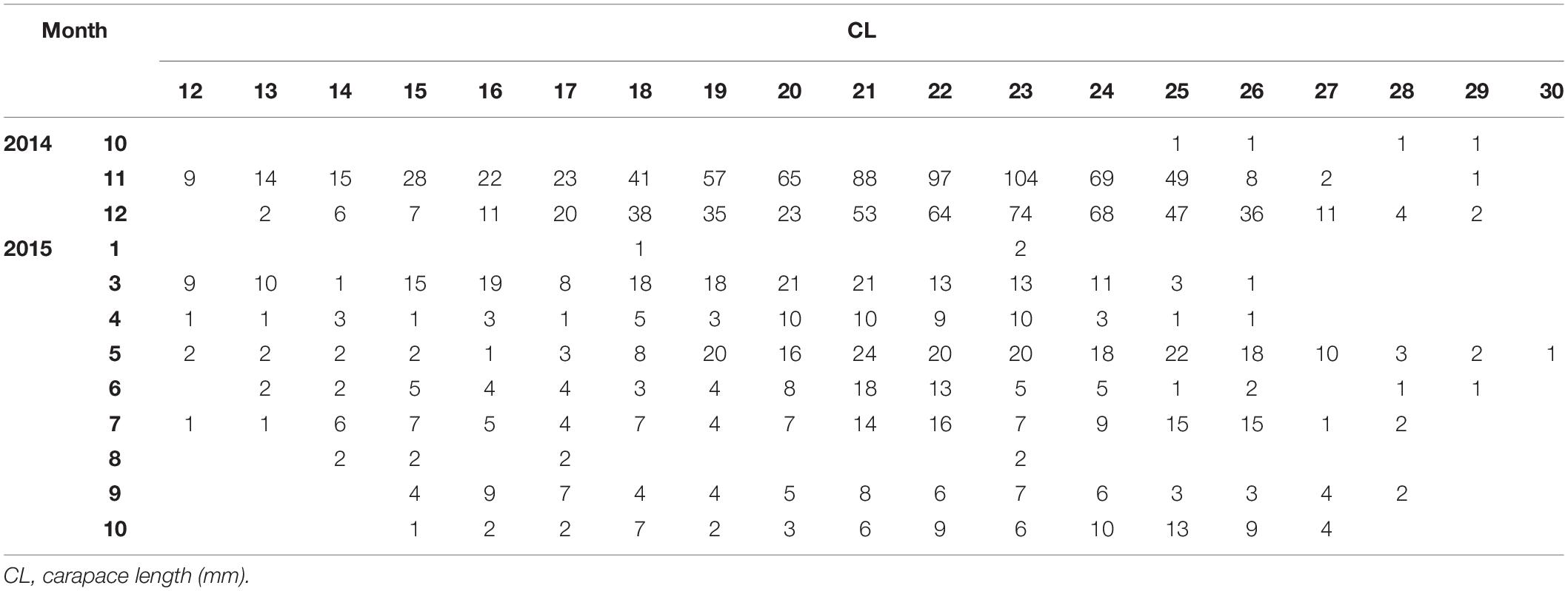
Table 1. Monthly (1: January – 12: December) length frequency of P. edwardsii in SE Aegean Sea during 2014–2015.

TABLE 2

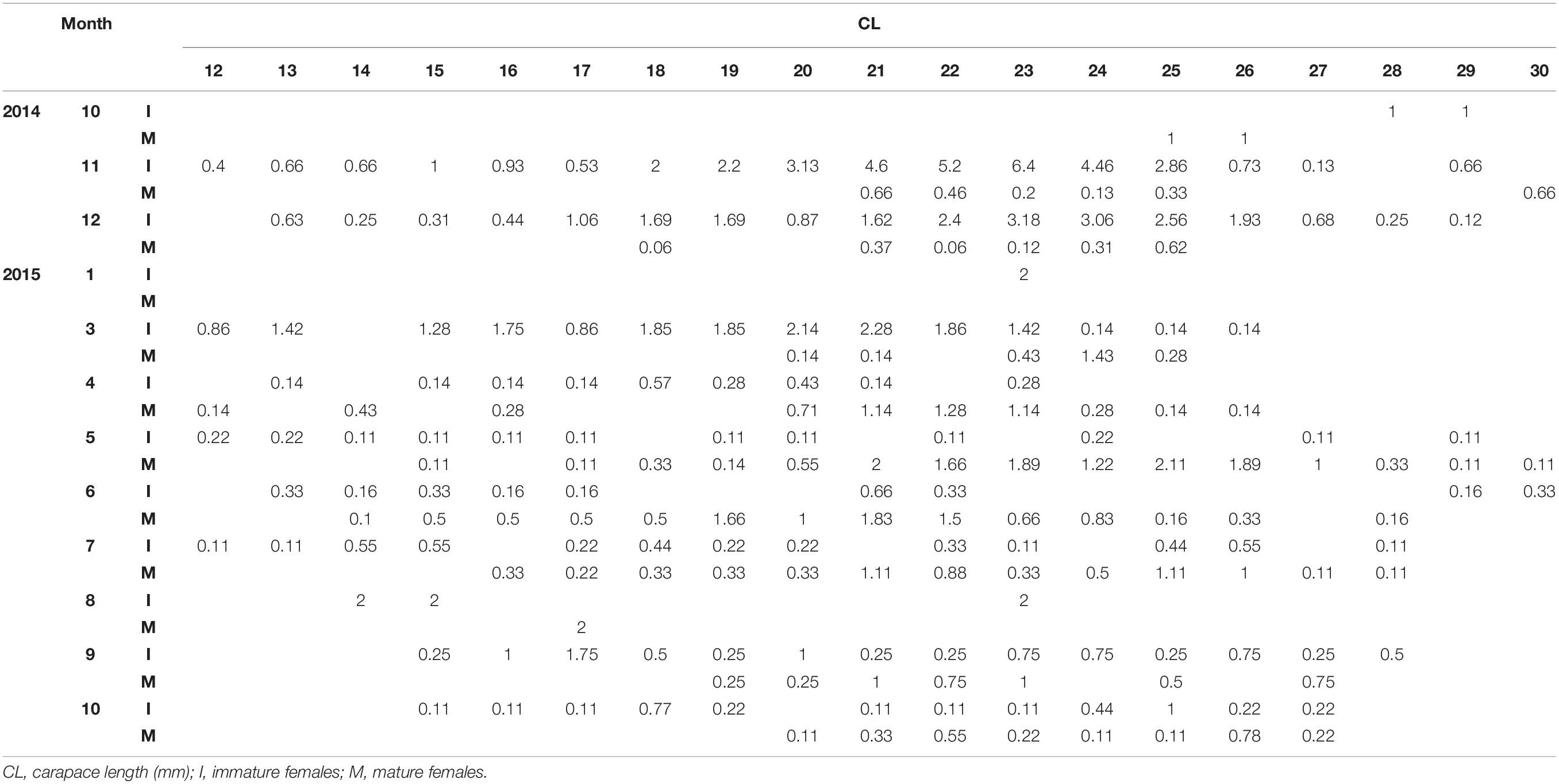
Table 2. Standardized monthly (1: January – 12: December) length frequency of mature and immature females of P. edwardsii in SE Aegean Sea during 2014–2015.

After standardizing the LFDs and examining separately mature and immature individuals, a dominance of mature females emerged between spring and mid-summer indicating a spawning period (Tables 1, 2).

Depth was found to be influential, with more individuals found in the deeper strata (Supplementary Figure 1). A dominance of females was evident at all depths with a sex ratio of 0.82 (Supplementary Figure 2), complemented by larger females (up to 30 mm) at increased depths (Supplementary Figures 3, 4). Mean size of males (19.83 mm CL) was lower than that of females (21.40 mm CL), with a maximum size of 26 mm.

Growth Parameters

Visualizing the raw and standardized LFQ data (Tables 1, 2 and Figure 3) showed that recruits to the fishery appear in March at a CL of ∼12 mm. After exploring possible months for t_anchor (Supplementary Figure 4), May was selected (t_anchor = 5/12) (Supplementary Figure 5). This month provided the best fit, and it was also when the higher fraction of mature females was observed.

FIGURE 3

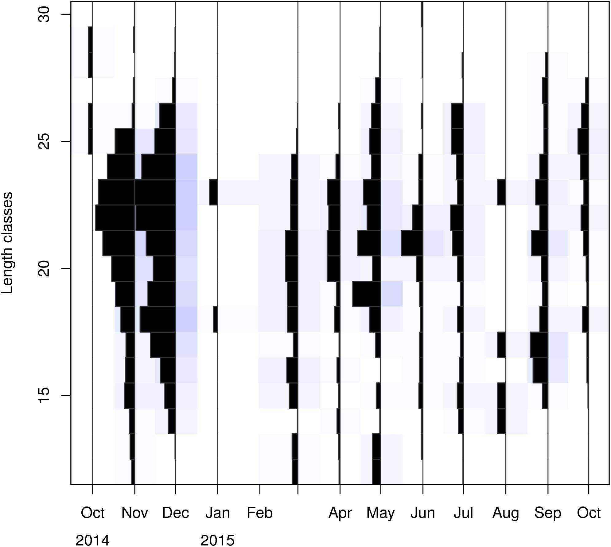
Figure 3. The LFDs analyzed by ELEFAN. Length classes (CL) are in mm.

L_inf estimations varied between the different methods used. L_inf was estimated at 26.64 mm by the Powell and Wetherall method (Supplementary Figure 5), at 44.13 mm by the Froese and Binohlan formula, while the maximum CL observed in the samples was 30.00 mm (Table 3). Although the Powell and Whetherall method estimation with MA = 7 got the highest Rn value (Table 3), its resulting VBGF parameter estimates were not retained. That was because the relevant L_inf estimation (27.24 mm) was underestimating the population’s true L_inf, being lower than the larger individuals sampled (30.00 mm) (Table 3). By contrast, the L_inf estimation by the Froese and Binohlan formula was found to be greater than the larger individuals sampled. Therefore, to select the optimal VBGF parameter estimates we focused on the two runs using the maximum length as a lower limit of the L_inf range (Table 3). Among these two runs, the one with a MA width of 5 bins had the highest Rn value and a t_anchor value closer to the assumed spawning period (Table 3). The final VBGF parameter estimates were: L_inf = 31.94 mm, K = 0.56 y^–1, t_anchor = 0.31 y (Figure 4). Five age cohorts were estimated by the VBGF model (Figure 5).

TABLE 3

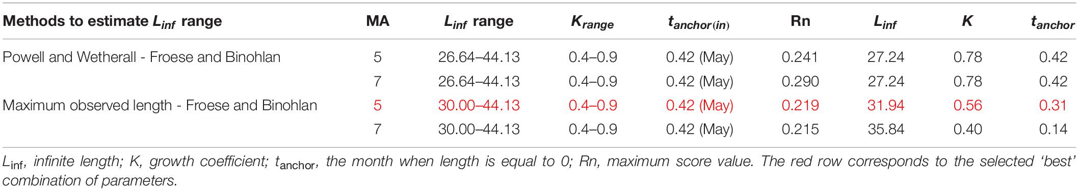
Table 3. Main settings adopted in running the ELEFAN analysis in terms of L_inf and K range, initial t_anchor value and Moving Average (MA) and main correspondent outputs.

FIGURE 4

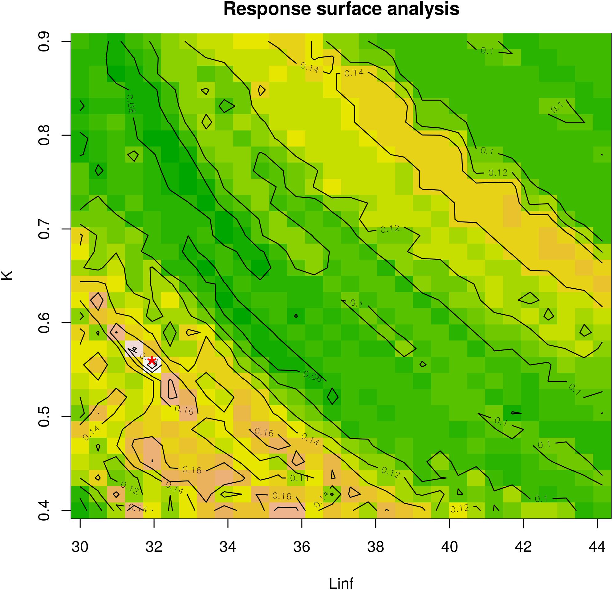
Figure 4. Response surface analysis. The best fit for the combination between Linf (in mm) and K-values is indicated with a red asterisk on the plot. The color scale corresponds to the Rn values from ELEFAN analysis. K ranges between 0.4 and 0.9 and L_inf ranges between 30 mm (maximum observed length) and 44.13 mm (estimated by Froese and Binohlan). This analysis corresponds to the optimal combination from Table 1.

FIGURE 5

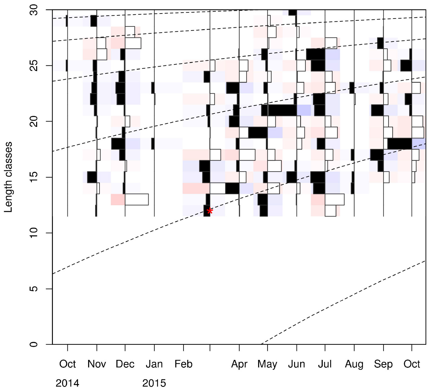
Figure 5. Age cohorts (dashed lines) estimated by the VBGF model. Red asterisk indicates the size at which the youngest individuals are captured. Length classes (CL) are in mm.

Total, Natural and Fishing Mortality

Z was estimated as 2.25 y^–1 by the LCCC method (Supplementary Figure 9) and 2.36 y^–1 by the Beverton and Holt formula. The sixteen different methods used for M, produced values ranging between 0.44 y^–1 (Alverson_Carney) and 2.01 y^–1 (Lorenzen) (Table 4). The combination of the two values of Z with 16 values of M produced 32 different values for F ranging between 0.24 y^–1 (Lorenzen) and 1.92 y^–1 (Alverson_Carney) (Table 4).

TABLE 4

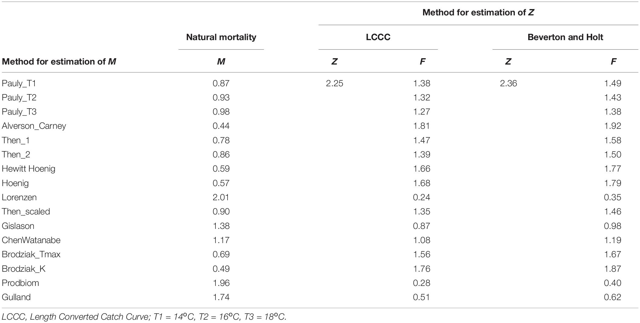
Table 4. Values of fishing, natural and total mortality as given by the equation: total mortality rate (Z) = natural mortality rate (M) + fishing mortality rate (F).

Stock Status

In total, only seven out of the 32 estimates of the exploitation state indicated sustainable levels of fishing both in terms of F and in terms of E (Figure 6). These included all six cases where the Lorenzen, ProdBiom and Gulland methods were used and one case where the Gislason method was used for the estimation of M. By contrast, 22 estimates of the exploitation state indicated overfishing, both in terms of F and in terms of E (Figure 5). These included all cases where the Pauly_T1, Pauly_T2, Pauly_T3, Alverson_Carney, Then_1, Then_2, Hoenig_1, Hoenig_2, Then_scaled, Brodziak_Tmax, and Brodziak_K methods were used for the estimation of M. In three cases, two using ChenWatanabe and one using Gislason for the estimation of M, the stock was found to be overfished in terms of E but non-overfished in terms of F. Both the mean and median stock status was estimated as overfished (Figure 6). In particular, for F/F_0.1 mean values were 1.68 (LCCC method) and 1.81 (Beverton and Holt formula) and median values were 1.43 and 1.56, respectively. For E/E_0.4 mean values were 1.36 and 1.42 and median values were 1.51 and 1.56 according to the previous sequence. Therefore, our results pointed toward a state of overfishing.

FIGURE 6

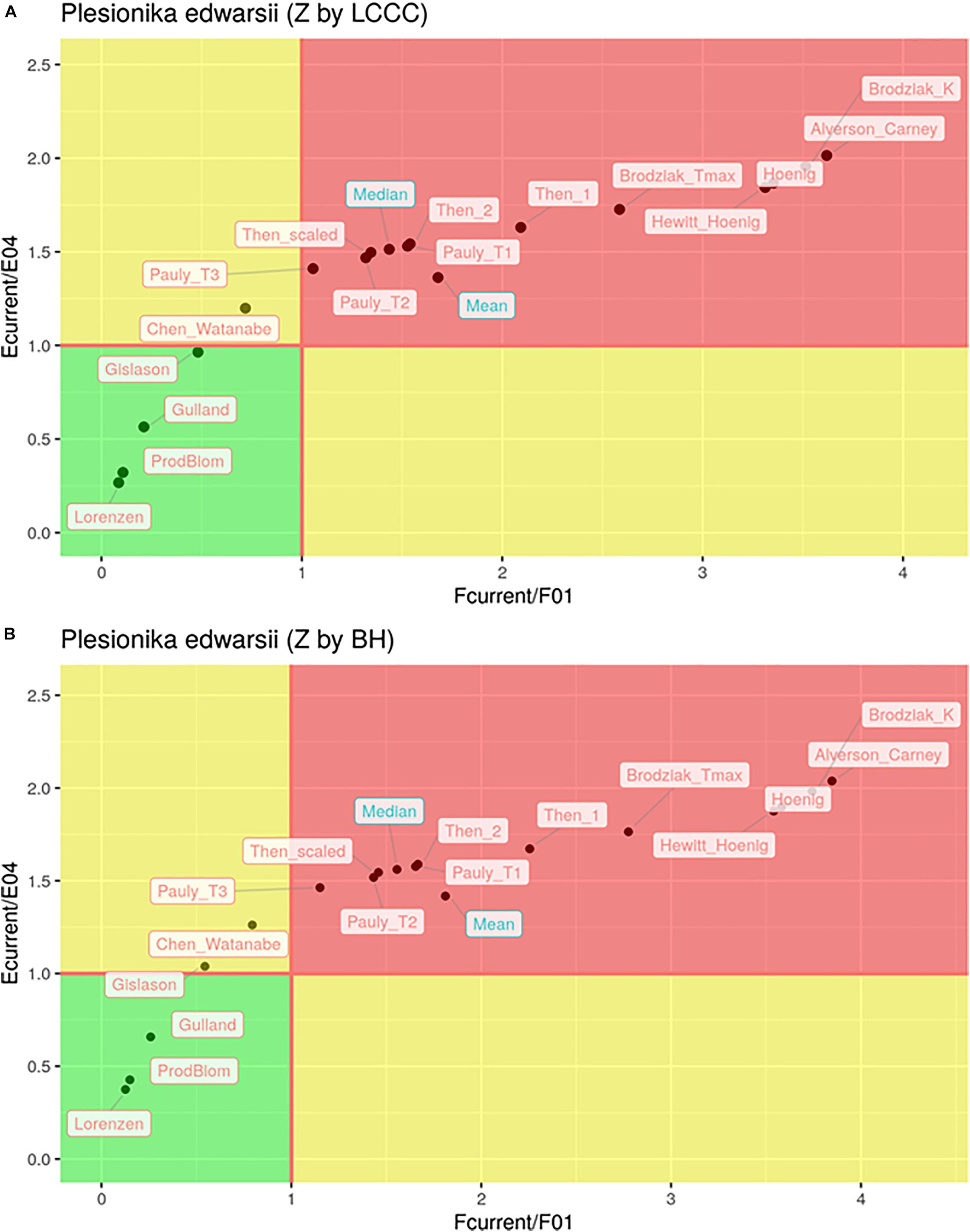
Figure 6. Kobe plot of $\frac{F}{F0.1}$ and $\frac{E}{E0.4}$ for different estimations of natural mortality (M) with total mortality (Z) estimated by LCCC (A) or the Beverton and Holt formula (B).

Results From LBB

Table 5 summarizes the main results from the LBB. L_inf ranged between 31.92 mm (Lorenzen) and 32.56 mm (Hoenig); M/K ranged from 0.96 (Alverson_Carney) to 3.60 (Lorenzen) and F/M ranged between 0.41 (Prodbiom) to 5.08 (Alverson_Carney). All these values were similar to ones obtained from our original analysis.

TABLE 5

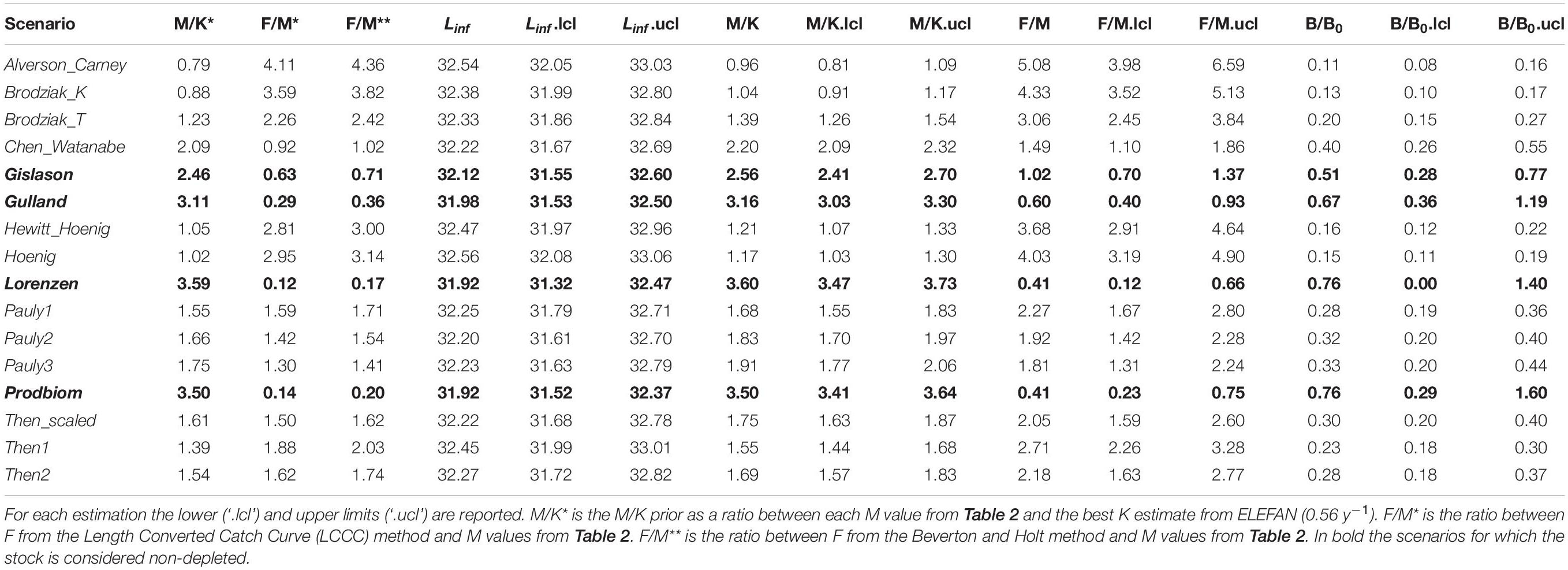
Table 5. Length-based Bayesian Biomass method (LBB) estimates of asymptotic length (L_inf), natural mortality relative to somatic growth rate (M/K), fishing mortality relative to natural mortality (F/M) and current biomass relative to unexploited biomass (B/B₀) by M scenario.

The exploitation status of P. edwarsii was estimated as non-depleted in three M scenarios (Gulland, Lorenzen and Prodbiom), close to equilibrium in one M scenario (Gislason) and as in moderate or severe depletion in all other scenarios (Table 5).

Discussion

This study proposes a stepwise methodological framework to assess stock status of an extremely data-limited exploited stock. Lack of data constitutes a common restrictive factor for fisheries management and the applied methods can be decisive for the outcomes. Our proposed framework is a sequence entailing estimations of basic life traits, mortality rates and biological reference points to infer stock status. The combination of high data uncertainty and multiple method availability (Gayanilo and Pauly, 1997) often lead to tradeoffs in the method(s) to be used. By contrast, the numerous estimates for the same variable offer the opportunity to calculate the average (weighted or not) of values instead of presenting a single-method prediction (Dormann et al., 2018). This is especially relevant when the analyzed data come from small-scale fisheries with low data availability, which are prevalent in the Mediterranean Sea.

The range of outputs estimated by this study underlines the necessity of a multi-method approach. For each of the steps presented in this study, a single method selection would be misleading and would constitute a sub-optimal methodological path selection. Previous studies on the biology of P. edwardsii stock (e.g., Colloca, 2002; González et al., 2016) used a single method approach but with much larger and balanced datasets and thus the relevant results were more reliable; however, these studies did not touch upon stock status. In our study, we use a multi-method approach through a stepwise process; the most pronounced example being the estimation of natural mortality rate (M) for which we used 16 different methods. Such a parallel implementation of several methods for M is not usually applied (Kenchington, 2014), and the M value is typically calculated using only one of a handful of M equations (e.g., Pauly, 1980; Hoenig, 1983). The wide range of our results demonstrates the great variability that exists across these 16 approaches used and the complexity of pinpointing the most suitable one. Using various M estimators is often recommended for reducing bias, errors, underestimations and uncertainties of the methods applied (Gunderson et al., 2003; Simpfendorfer et al., 2005). Notably, the range of outputs produced when using our proposed framework was similar to that observed when implementing the novel LBB method (Froese et al., 2018). This highlights how in extremely data-limited situations the choices made with regards to key input parameters (such as M) have a greater impact on the outputs than the analytical method used.

Ensemble modeling use several options and generates more robust outputs. Selection of the most appropriate method may often prove to be more difficult than initially expected because the theoretical and/or empirical background is not precise enough. Applying ensemble modellin is recommended in extremely data-limited situations, because various models can be used for estimating a value and all results can be statistically tested (Kuhn and Johnson, 2013). Using model averaging to infer stock status could be a sufficient solution for decreasing the predicted error. When models are unbiased and with high variance, using an increasing number of different models could minimize the error (Dormann et al., 2018). An alternative to using a simple model mean or median, as used in this study, would be to use a weighted average. Not all estimators may be equally reliable; e.g., some of the M estimators used here may be more suitable for fish than crustaceans. In such cases, a weighted estimation could provide more accurate results (Kenchington, 2014; Dormann et al., 2018).

Extremely data-limited stocks often have a high importance for both fisheries and the marine ecosystem; hence one should strive for analytical examinations to infer stock status. However, the use of a multi-method approach alone does not provide certainty about the real situation in extremely data-limited situations. The analytical framework proposed here, when applied to extremely data-limited stocks, it should be viewed as the first stage of exploration; a starting point to reveal stock status. Next steps should involve a more extensive data collection so that the initial insights could be corroborated or rejected. In the meanwhile, controlling size selectivity and safeguarding stock productivity constitute a sound strategy for the management of extremely data-limited stocks (Prince and Hordyk, 2019), especially in areas such as the Mediterranean Sea which are known to be severely overfished (Vasilakopoulos et al., 2014).

The same principles of better monitoring and precautionary measures also apply to the Dodecanese P. edwardsii stock used as a case study here. Our study suggests that the P. edwardsii stock is likely overfished, in line with its sympatric P. narval stock (Maravelias et al., 2018) and most other assessed crustacean stocks in the Mediterranean Sea (Vasilakopoulos and Maravelias, 2016). In this context, the managers of the P. narval fishery need to strive for better monitoring of the bycatch P. edwardsii to obtain a better understanding of its status; e.g., by carrying out targeted sampling in deeper strata where P. edwardsii is known to be more abundant than P. narval. If the overexploited state of P. edwardsii is confirmed, management plans for P. narval should take into consideration the state of P. edwardsii as well and adjust the fishing activities accordingly.

This study provides a stepwise analytical methodology to be applied to any extremely data-limited stock. The range of methods that we have used in each step is not exhaustive and fisheries scientists are encouraged to use more and/or different methods according to the specific characteristics of the stock at hand. Inferring the stock status of extremely data-limited stocks usually involves unique challenges in every individual case; nevertheless, we are confident that following part or all of the methodological steps proposed here can prove extremely helpful.

Data Availability Statement

The raw data supporting the conclusions of this article will be made available by the authors, without undue reservation.

Author Contributions

SK, VP, PV, and PM conceived the study. SK and KK contributed to the data collection. AM and VP did the analysis. VP, AM, PV, and SK interpreted the results. VP led the writing of the manuscript with input from all authors. All the authors contributed to the article and approved the submitted version.

Funding

This work was supported by the Greek Operational Programme “Fisheries 2007-2013” [grant number 185366, 2014] approved by the European Commission with decision no. E(2007)6402/11-122007, Programme reference No. CCI:2007GR14FPO001.

Conflict of Interest

The authors declare that the research was conducted in the absence of any commercial or financial relationships that could be construed as a potential conflict of interest.

Supplementary Material

The Supplementary Material for this article can be found online at: https://www.frontiersin.org/articles/10.3389/fmars.2020.583148/full#supplementary-material

References

Abella, A. J., Caddy, J. F., and Serena, F. (1997). Do natural mortality and availability decline with age? An alternative yield paradigm for juvenile fisheries, illustrated by the hake Merluccius merluccius fishery in the Mediterranean. Aqua. Liv. Resour. 10, 257–269. doi: 10.1051/alr:1997029

CrossRef Full Text | Google Scholar

Alverson, D. L., and Carney, M. J. (1975). A graphic review of the growth and decay of population cohorts. ICES J. Mar. Sci. 36, 133–143. doi: 10.1093/icesjms/36.2.133

CrossRef Full Text | Google Scholar

Beare, D. J., Needle, C. L., Burns, F., and Reid, D. G. (2005). Using survey data independently from commercial data in stock assessment: an example using haddock in ICES Division VIa. ICES J. Mar. Sci. 62, 996–1005. doi: 10.1016/j.icesjms.2005.03.003

CrossRef Full Text | Google Scholar

Beverton, R. J. H., and Holt, S. J. (1956). A review of the methods for estimating mortality rates in fish populations, with special reference to sources of bias in catch sampling. Rapp. P. V. Réun. Cons. Int. Explor. Mer. 140, 67–83.

Google Scholar

Beverton, R. J. H., and Holt, S. J. (1957). On the dynamics of exploited fish populations. Great Britain: Ministry of Agriculture.

Google Scholar

Brodziak, J., Ianelli, J., Lorenzen, K., and Methot, R. D. Jr. (2011). Estimating natural mortality in stock assessment applications. Department Commerce, NOAA, Tech Memo, NMFS-F/SPO-199, NMFS-F/SPO-199pg. (Washington: NOAA), 38.

Google Scholar

Caddy, J. F. (1991). Death rates and time intervals: is there an alternative to the constant natural mortality axiom? Rev. Fish Biol. Fish. 1, 109–138. doi: 10.1007/BF00157581

CrossRef Full Text | Google Scholar

Caddy, J. F., and Mahon, R. (1995). Reference points for fisheries management. FAO Fisher. Tech. Pap. 347:83.

Google Scholar

Chen, S., and Watanabe, S. (1989). Age Dependence of Natural Mortality Coefficient in Fish Population Dynamics. Nipp. Suis. Gakka. 55, 205–208. doi: 10.2331/suisan.55.205

CrossRef Full Text | Google Scholar

Colloca, F. (2002). Life Cycle of the Deep-Water Pandalid Shrimp Plesionika edwardsii (Decapoda, Caridea) in the Central Mediterranean Sea. J. Crust. Biol. 22, 775–783. doi: 10.1651/0278-0372(2002)022[0775:lcotdw]2.0.co;2

CrossRef Full Text | Google Scholar

Company, J. B., and Sardà, F. (2000). Growth parameters of deep-water decapod crustaceans in the Northwestern Mediterranean Sea: a comparative approach. Mar. Biol. 136, 79–90. doi: 10.1007/s002270050011

CrossRef Full Text | Google Scholar

Dormann, C. F., Calabrese, J. M., Guillera-Arroita, G., Matechou, E., Bahn, V., Bartoñ, K., et al. (2018). Model averaging in ecology: a review of Bayesian, information-theoretic, and tactical approaches for predictive inference. Ecol. Monogr. 88, 485–504. doi: 10.1002/ecm.1309

CrossRef Full Text | Google Scholar

Froese, R. (2004). Keep it simple: three indicators to deal with overfishing. Fish Fisher. 5, 86–91. doi: 10.1111/j.1467-2979.2004.00144.x

CrossRef Full Text | Google Scholar

Froese, R., and Binohlan, C. (2000). Empirical relationships to estimate asymptotic length, length at first maturity and length at maximum yield per recruit in fishes, with a simple method to evaluate length frequency data. J. Fish Biol. 56, 758–773. doi: 10.1111/j.1095-8649.2000.tb00870.x

CrossRef Full Text | Google Scholar

Froese, R., Demirel, N., Coro, G., Kleisner, K. M., and Winker, H. (2017). Estimating fisheries reference points from catch and resilience. Fish Fisher. 18, 506–526. doi: 10.1111/faf.12190

CrossRef Full Text | Google Scholar

Froese, R., Stern-Pirlot, A., Winker, H., and Gascuel, D. (2008). Size matters: How single-species management can contribute to ecosystem-based fisheries management. Fisher. Res. 92, 231–241. doi: 10.1016/j.fishres.2008.01.005

CrossRef Full Text | Google Scholar

Froese, R., Winker, H., Coro, G., Demirel, N., Tsikliras, A. C., Dimarchopoulou, D., et al. (2018). A new approach for estimating stock status from length frequency data. ICES J. Mar. Sci. 75, 2004–2015. doi: 10.1093/icesjms/fsy078

CrossRef Full Text | Google Scholar

Fryer, R. F., Needle, C. L., and Reeves, S. A. eds. (1998). “Kalman filter assessments of cod, haddock and whiting in VIa,” in Working Document WD1 to the ICES Working Group on the Assessment of Northern Shelf Demersal Stocks, (Copenhagen: ICES).

Google Scholar

García-Rodriguez, M., Esteban, A., and Perez Gil, J. L. (2000). Considerations on the biology of Plesionika edwardsi (Brandt, 1851) (Decapoda, Caridea, Pandalidae) from experimental trap catches in the Spanish western Mediterranean Sea. Scient. Mar. 64, 369–379. doi: 10.3989/scimar.2000.64n4369

CrossRef Full Text | Google Scholar

Gayanilo, F. C., and Pauly, D. eds. (1997). “FAO-ICLARM Stock Assessment Tools: Reference Manual,” in FAO Computerized Information Series (Fisheries) 8, (Rome: Food and Agriculture Organization of the United Nations).

Google Scholar

Gislason, H., Daan, N., Rice, J. C., and Pope, J. G. (2010). Size, growth, temperature and the natural mortality of marine fish. Fish Fisher. 11, 149–158. doi: 10.1111/j.1467-2979.2009.00350.x

CrossRef Full Text | Google Scholar

González, J. A., Pajuelo, J. G., Triay-Portella, R., Ruiz-Díaz, R., Delgado, J., Góis, A. R., et al. (2016). Latitudinal patterns in the life-history traits of three isolated Atlantic populations of the deep-water shrimp Plesionika edwardsii (Decapoda, Pandalidae). Deep Sea Res. Part I Oceanogr. Res. Pap. 117, 28–38. doi: 10.1016/j.dsr.2016.09.004

CrossRef Full Text | Google Scholar

Gulland, J. A. (1965). “Estimation of mortality rates,” in Annex to Arctic Fisheries Working Group Report.(ICES Council Meeting papers), (Cambridge: ICES Gadoid Fish.Comm).

Google Scholar

Gulland, J. A., and Boerema, L. K. (1973). Scientific advice on catch levels. Fisher. Bull. 71, 325–335.

Google Scholar

Gunderson, D. R., Zimmermann, M., Nichol, D. G., and Pearson, K. (2003). Indirect estimates of natural mortality rate for arrowtooth flounder (Atheresthes stomias) and dark-blotched rockfish (Sebastes crameri). Fisher. Bull. 101, 175–182.

Google Scholar

Hewitt, D. A., and Hoenig, J. M. (2005). Comparison of two approaches for estimating natural mortality based on longevity. Fisher. Bull. 103, 433–437.

Google Scholar

Hoenig, J. M. (1983). Empirical Use of Longevity Data to Estimate Mortality Rates. Fisher. Bull. 82, 898–903.

Google Scholar

ICES (2008). Report of the Working Group on the Assessment of Northern Shelf Demersal Stock (WGNSDS), 15-21 May 2008, ICES CM 2008/ACOM 08, Copenhagen, 757.

Google Scholar

ICES (2012). ICES Implementation of Advice for Data-limited Stocks in 2012 in its 2012 Advice. ICES CM 2012/ACOM, Copenhagen, 68, 42.

Google Scholar

Kalogirou, S., Anastasopoulou, A., Kapiris, K., Maravelias, C. D., Margaritis, M., Smith, C., et al. (2017). Spatial and temporal distribution of narwal shrimp Plesionika narval (Decapoda, Pandalidae) in the Aegean Sea (eastern Mediterranean Sea). Reg. Stud. Mar. Sci. 16, (Suppl. C), 240–248. doi: 10.1016/j.rsma.2017.09.014

CrossRef Full Text | Google Scholar

Kalogirou, S., Pihl, L., Maravelias, C. D., Herrmann, B., Smith, C. J., Papadopoulou, N., et al. (2019). Shrimp trap selectivity in a Mediterranean small-scale-fishery. Fisher. Res. 211, 131–140. doi: 10.1016/j.fishres.2018.11.006

CrossRef Full Text | Google Scholar

Kenchington, T. J. (2014). Natural mortality estimators for information-limited fisheries. Fish Fisher. 15, 533–562. doi: 10.1111/faf.12027

CrossRef Full Text | Google Scholar

Kuhn, M., and Johnson, K. (2013). Applied predictive modeling. Berlin: Springer.

Google Scholar

Lorenzen, K. (2000). Allometry of natural mortality as a basis for assessing optimal release size in fish-stocking programmes. Can. J. Fisher. Aqua. Sci. 57, 2374–2381. doi: 10.1139/f00-215

CrossRef Full Text | Google Scholar

Mannini, A., Pinto, C., Konrad, C., Vasilakopoulos, P., and Winker, H. (in review). The elephant in the room’: Exploring natural mortality uncertainty in statistical catch at age models. Front. Mar. Sci.

Google Scholar

Maravelias, C. D., Vasilakopoulos, P., Kalogirou, S., and Handling Raúl, P. (eds) (2018). Participatory management in a high value small-scale fishery in the Mediterranean Sea. ICES J. Mar. Sci. 75, 2097–2106. doi: 10.1093/icesjms/fsy119

CrossRef Full Text | Google Scholar

Martell, S., and Froese, R. (2013). A simple method for estimating MSY from catch and resilience. Fish Fisher. 14, 504–514. doi: 10.1111/j.1467-2979.2012.00485.x

CrossRef Full Text | Google Scholar

Martiradonna, A. (2012). Modelli di dinamica delle popolazioni ittiche: stima dei fattori di incremento e decremento dello stock. Italy: Università di Bari.

Google Scholar

Meyer, R., and Millar, R. B. (1999). BUGS in Bayesian stock assessments. Can. J. Fisher. Aqua. Sci. 56, 1078–1087. doi: 10.1139/f99-043

CrossRef Full Text | Google Scholar

Mildenberger, T. K., Taylor, M. H., and Wolff, M. (2017). TropFishR: an R package for fisheries analysis with length-frequency data. Methods Ecol. Evol. 8, 1520–1527. doi: 10.1111/2041-210X.12791

CrossRef Full Text | Google Scholar

Patterson, K. (1992). Fisheries for small pelagic species: an empirical approach to management targets. Rev. Fish Biol. Fisher. 2, 321–338. doi: 10.1007/BF00043521

CrossRef Full Text | Google Scholar

Pauly, D. (1980). On the interrelationships between natural mortality, growth parameters, and mean environmental temperature in 175 fish stocks. ICES J. Mar. Sci. 39, 175–192. doi: 10.1093/icesjms/39.2.175

CrossRef Full Text | Google Scholar

Pauly, D. (1985). On Improving Operation and Use of the ELEFAN Programs. Part 1, Avoiding Drift of K Towards Low Values. Fishbyte 11, 13–14.

Google Scholar

Pauly, D. (1990). Length-Converted Catch Curves and the Seasonal Growth of Fishes. Fishbyte 8, 24–29.

Google Scholar

Pauly, D., and David, N. (1981). ELEFAN I, a BASIC program for the objective extraction of growth parameters from length-frequency data. Berich der Deutschen WissenschafHichen Kommission fiir Meeresforschung 28, 205–211.

Google Scholar

Pedersen, M. W., and Berg, C. W. (2017). A stochastic surplus production model in continuous time. Fish Fisher. 18, 226–243. doi: 10.1111/faf.12174

CrossRef Full Text | Google Scholar

Polacheck, T., Hilborn, R., and Punt, A. E. (1993). Fitting Surplus Production Models: Comparing Methods and Measuring Uncertainty. Can. J. Fisher. Aqua. Sci. 50, 2597–2607. doi: 10.1139/f93-284

CrossRef Full Text | Google Scholar

Powell, D. G. (1979). Estimation of mortality and growth parameters from the length frequency of a catch [model]. Rapp. Proc. Verb. Reun. 175, 167–169.

Google Scholar

Prince, J., and Hordyk, A. (2019). What to do when you have almost nothing: A simple quantitative prescription for managing extremely data-poor fisheries. Fish and Fisheries 20, 224–238. doi: 10.1111/faf.12335

CrossRef Full Text | Google Scholar

Punt, A. E. (2003). Extending production models to include process error in the population dynamics. Can. J. Fisher. Aqua. Sci. 60, 1217–1228. doi: 10.1139/f03-105

CrossRef Full Text | Google Scholar

R Core Team. (2020). R: A language and environment for statistical computing. URL https://www.R-project.org/, (Vienna: R Foundation for Statistical Computing).

Google Scholar

Santana, J. I., Gonzales, J. A. A., Lozano, I. J., and Tuset, V. M. (1997). Life history of Plesionika edwardsii (Crustacea, Decapoda, Pandalidae) around the Canary Islands, Eastern Central Atlantic. Afr. J. Mar. Sci. 18, 39–48. doi: 10.2989/025776197784161045

CrossRef Full Text | Google Scholar

Schwamborn, R. (2018). How reliable are the Powell–Wetherall plot method and the maximum-length approach? Implications for length-based studies of growth and mortality. Rev. Fish Biol. Fisher. 28, 587–605. doi: 10.1007/s11160-018-9519-0

CrossRef Full Text | Google Scholar

Simpfendorfer, C. A., Bonfil, R., Latour, R. J., Musick, J. A., and Bonfil, R. (2005). “Mortality estimation,” in Management Techniques for Elasmobranch Fisheries, eds Edn, Vol. 474, (FAO Fisheries Technical Paper), 127–142.

Google Scholar

STECF (17-15) (2017). Scientific, Technical and Economic Committee for Fisheries (STECF) - Mediterranean Stock Assessments 2017 part I (STECF-17-15). (Luxembourg: Publications Office of the European Union), ISBN 978-92-79-67487-7.

Google Scholar

STECF (19-16) (2019). Scientific, Technical and Economic Committee for Fisheries (STECF) - Stock Assessments: demersal stocks in the western Mediterranean Sea (STECF-19-10). (Luxembourg: Publications Office of the European Union), ISBN 978-92-76-11288-4.

Google Scholar

STECF (2020). Scientific, Technical and Economic Committee for Fisheries (STECF) - Monitoring the Performance of the Common Fisheries Policy (STECF-Adhoc-20-01). (Luxembourg: Publications Office of the European Union), ISBN 978-92-76-18115-6. doi: 10.2760/230469

CrossRef Full Text | Google Scholar

Taylor, M. H., and Mildenberger, T. K. (2017). Extending electronic length frequency analysis in R. Fisher. Manag. Ecol. 24, 330–338. doi: 10.1111/fme.12232

CrossRef Full Text | Google Scholar

Then, A. Y., Hoenig, J. M., Hall, N. G., Hewitt, D. A., and Jardim, H. E. E. (2014). Evaluating the predictive performance of empirical estimators of natural mortality rate using information on over 200 fish species. ICES J. Mar. Sci. 72, 82–92. doi: 10.1093/icesjms/fsu136

CrossRef Full Text | Google Scholar

Vasilakopoulos, P., and Maravelias, C. D. (2016). A tale of two seas: A meta-analysis of crustacean stocks in the NE Atlantic and the Mediterranean Sea. Fish Fisher. 17, 617–636. doi: 10.1111/faf.12133

CrossRef Full Text | Google Scholar

Vasilakopoulos, P., Maravelias, C. D., Anastasopoulou, A., Kapiris, K., Smith, C. J., and Kalogirou, S. (2019). Premium small scale: the trap fishery for Plesionika narval (Decapoda, Pandalidae) in the eastern Mediterranean Sea. Hydrobiologia 826, 279–290. doi: 10.1007/s10750-018-3739-0

CrossRef Full Text | Google Scholar

Vasilakopoulos, P., Maravelias, C. D., and Tserpes, G. (2014). The alarming decline of Mediterranean fish stocks. Curr. Biol. 24, 1643–1648. doi: 10.1016/j.cub.2014.05.070

PubMed Abstract | CrossRef Full Text | Google Scholar

Wetherall, J. A., Polovina, J. J., and Ralston, S. (1987). Estimating growth and mortality in steady-state fish stocks from length-frequency data. ICLARM Conf. Proc. 13, 53–74.

Google Scholar