Sea Turtles for Ocean Research and Monitoring: Overview and Initial Results of the STORM Project in the Southwest Indian Ocean

Introduction

Because sea temperature has a strong influence on climate dynamics and global transport of ocean water masses, knowledge and observation of this parameter is fundamental to achieve realistic forecasts and simulations of the coupled ocean-atmosphere system at all spatial and temporal scales. In particular, sea surface temperature (SST) is an essential parameter in meteorology and oceanography, especially in tropical regions, where it plays a major role in the formation of tropical low-pressure systems, and more generally, ocean-atmosphere interactions.

In recent decades, the international community has developed the Global Ocean Observing System (GOOS, Zhang et al., 2009), which has subsequently been integrated into the Global Climate Observing System (GCOS). Resulting satellite measurements have significantly improved the space-time coverage of ocean observations, contributing to the reduction of sampling and other random errors in sea surface temperature (SST) analyses. However, these measurements remain subject to significant biases that need to be corrected by drifting or moored buoys to minimize systematic errors in data analyses (Zhang et al., 2006).

In the equatorial zone, the Research Moored Array for African-Asian-Australian Monsoon Analysis and Prediction (RAMA) network (McPhaden et al., 2009), which comprises about 40 moored buoys spread along the tropical belt, is a key element of the GOOS observing system. RAMA buoys effectively complement the network of surface drifting buoys deployed in the tropics by collecting temperature and salinity measurements down to 500 m depth. The advent, in the early 2000s, of the Argo profiling network (Davis et al., 2001), consisting of drifting bathymetric sounders that routinely descend to 2,000 m, is another major step forward in sampling the surface and subsurface properties of the oceans worldwide. With more than 3,800 systems from 30 different contributing countries as of July 2020, the ARGO network has thus become not only the world’s main source of knowledge for oceanographic studies, but also the main source of data for calibrating and verifying temperature, salinity and velocity fields derived from satellite observations and numerical ocean model predictions.

Although the ARGO and RAMA networks have significantly improved the density and quality of measurements in the tropical oceans, their coverage is not uniform and not always optimized for short- and medium-term applications. The sampling frequency of ARGO drifters (1 profile every 10 days on average) is, for instance, rather low and the spatial resolution of the RAMA network (5–15° zonal resolution) is quite loose, especially in the Southwest Indian Ocean (SWIO). With the continued deployment of new drifters, mooring buoys and satellite missions, the coverage of ocean observations is nevertheless expected to further improve considerably in the coming years. However, because of the extensive development and maintenance costs associated with such programs, researchers have also been considering new measurement capabilities to improve and complement existing observing networks at lower cost.

An appealing alternative for collecting oceanic data over periods ranging from a few days to several years is to use marine animals equipped with biologgers (aka bio-logging), that is electronic tags equipped with various environmental sensors. Animal-borne systems are indeed relatively inexpensive to operate compared to conventional observation systems (gliders, ARGO floats, ships). They can be deployed worldwide with limited human resources and therefore, used to extend ocean observations to remote and hard-to-reach areas. Furthermore, bio-logging also provides countries with limited human and financial resources the opportunity to contribute significantly to the collection of ocean observations. In this regard, animal-borne observations do not only provide unique and essential ocean data, but also have a positive impact on empowerment. Among the numerous marine candidate species available, air-breathing diving predators such as elephant seals (Cazau et al., 2017) have been considered the most attractive animals so far because of their mobility (wide migration), their large size (allowing them to be equipped with accurate geolocation and environmental sensors), and their ability to dive deep and frequently in the ocean (to collect numerous hydrographic profiles). Observations collected by elephant seals have been distributed for many years by the French Observation Service Mammifères marins Echantillonneurs du Milieu Océanique (MEMO), which subsequently joined the international consortium Marine Mammals Exploring the Oceans Pole to Pole (MEOP, Roquet et al., 2014). These data are regularly exploited by MERCATOR-Ocean, the United Kingdom MET-Office and the European Centre for Medium-Range Weather Forecasts (ECMWF) to improve ocean forecasting (through data assimilation) and monitor the state of the oceans, particularly in the polar gyres (Roquet et al., 2013). A drawback of this well-known biologging application is that elephant seals only evolve in high latitude areas, which excludes the possibility of making such measurements in tropical or mid-latitude regions. Another limitation, which nevertheless applies to all marine animals, is that collected measurements are solely made on the basis of the animals’ journeys and cannot be precisely based on pre-planned sampling strategies. This drawback can nevertheless be overcome by increasing the number of equipped animals in order to maximize the chances of sampling a given area.

The use of other marine animal species for collecting ocean data is attracting increasing interest from the international scientific community. For example, March et al. (2020) have recently explored the possibility of integrating measurements made by various marine animals (e.g., fish, cetaceans, turtles, penguins, etc.) into global ocean observing networks. While elephant seals, and more generally pinnipeds, appear to be well-suited to sample high latitude oceans, sea turtles (ST) also emerge as very good candidates to sample low- to mid-latitude oceanic areas.

The deployment of Argos tags on ST is a common and well-controlled procedure that has been used for more than 20 years to track the movements of all ST species worldwide (Godley et al., 2008). Satellite tracking is particularly well-suited to study key stages in the life cycle of these animals, knowledge of which is essential to improve their conservation (Jeffers and Godley, 2016). However, the use of ST to collect environmental ocean data is relatively recent. Although a first experiment was conducted in the North Atlantic as early as 2003 by McMahon et al. (2005), this approach was neglected for a while before being recently revived in three recent studies taking advantage of new advances in satellite telemetry and sensor miniaturization. Patel et al. (2018) used temperature measurements collected by loggerheads (Caretta caretta) to sample the ocean structure in a highly stratified region of the North-Eastern US continental shelf (Atlantic Ocean), while Miyazawa et al. (2019) and Doi et al. (2019) evaluated the benefits of assimilating temperature data collected by loggerhead and Olive Ridley (Lepidochelys olivacea) STs to improve regional ocean predictions in the Pacific Ocean.

In the tropical Indian Ocean, ST measurements were initiated in January 2019 as part of the INTERREG-V Indian Ocean 2014–2020 research project “ReNovRisk-Cyclones,” with the aim of assessing the relevance of such observations for ocean monitoring and modeling in the Southwest Indian Ocean (SWIO). During this experiment, conducted by Laboratory of Atmosphere and Cyclones (LACy), Centre d’Etude et de Découverte des Tortues Marines (CEDTM) and Kelonia, the Marine Turtle Observatory of Reunion Island, a dozen of rehabilitated loggerhead and Olive Ridley STs were equipped with Argos tags integrating TD (temperature/depth) sensors, before being released from Reunion Island. The preliminary results obtained during this experiment, presented hereafter, have confirmed the potential of this approach for oceanic studies, and led to the creation of the international research program “Sea Turtle for Ocean Research and Monitoring” (STORM).

The SWIO is home of significant cyclonic activity that regularly, and often dramatically, affects the inhabitants along the East African coast as well as over small (e.g., Reunion, Mauritius, Seychelles) and large (e.g., Madagascar) islands of this region. This basin, the second to third most active ocean basin in terms of cyclonic activity (Mavume et al., 2008; Matyas, 2015; Leroux et al., 2018), accounts for ∼10–12% of the global cyclonic activity, with an average of 10.5 storms per year. Although the conditions required for tropical cyclogenesis to occur are more or less the same in all ocean basins, the specific environments in which pre-existing perturbations evolve into warm-core cyclonic circulations can be locally very different due to the influence of large-scale climate anomalies (e.g., El Niño Southern Oscillation, Indian Ocean Dipole) and intra-seasonal variability (e.g., Madden Julian Oscillation). In this respect, the SWIO is one of the regions of the world where intra-seasonal atmospheric variability is associated with the strongest oceanic response and vice versa. The high prevalence of ocean-atmosphere interactions in this region is mainly related to the unique thermocline structure in the Seychelles-Chagos region (55–70°E, 5–15°S). In this area, also known as the Seychelles-Chagos Thermocline Ridge (SCTR), the thermocline is indeed particularly shallow (Hermes and Reason, 2008, 2009; Yokoi et al., 2008), which both favors strong SST response to atmospheric perturbations (Vialard et al., 2008) and modulates the ocean heat content that partly determines the spatial distribution of tropical cyclones (Xie et al., 2002).

Although the advent of coupled ocean-atmosphere models is a major achievement in improving TC forecasts on all time scales (e.g., Eyring et al., 2016; Vitart et al., 2017; Bousquet et al., 2020), these systems nevertheless constantly require new observations to constrain and evaluate the performance of their atmospheric and oceanic components. In this respect, the main objectives of the STORM project are twofold: (i) to document the ability of instrumented STs to sample the state of the Western Tropical Indian Ocean at high space-time resolution, and (ii) to evaluate the use of these datasets to assess and improve the performance of numerical ocean models, with emphasis on short- and medium-term time scales. From a biological perspective, STORM also aims to address key gaps in the spatial ecology of STs in the Western Indian Ocean, such as habitat characterization, assessment of adult migration routes and juvenile dispersal schemes, among others.

In this study, ∼115,000 temperature observations collected by loggerhead and Olive Ridley STs released from Reunion Island (55.28°E; 21.15°S) are compared to conventional ocean temperature datasets (ARGO, satellites), and used as an independent observational source to evaluate ocean model temperature forecasts. The paper is organized as follows: Section “Sea Turtle Observations” describes the data collection procedures, processing methods and spatial distribution of observations collected during the preliminary phase of STORM (January 2019–April 2020). The accuracy of temperature observations collected by STs is assessed in section “Evaluation of Sea Turtle Temperature Measurements” through comparisons with in situ (ARGO) in-depth data and satellite-derived SST datasets. In section “Evaluation of GLO12 Temperature Forecasts in the Tropical Western Indian Ocean,” surface and subsurface ST-borne observations are used to evaluate temperature fields simulated by the Ocean General Circulation Model (OGCM) “Glo12” (Lellouche et al., 2018) of the Copernicus Marine Environment Monitoring Service (CMEMS) in the western tropical Indian Ocean. Finally, section “Conclusions, Discussion, and Perspectives” describes the upcoming extension of STORM to the whole SWIO basin and discusses further applications to be carried out in the next phases of this research program.

Sea Turtle Observations

Capture

All sea turtles equipped in this study are juvenile specimens that were accidentally hooked by longliners in the vicinity of Reunion Island. In addition to hooking, the main sources of injury are caused by boat propellers, plastic ingestion or entanglement in large pieces of plastic (Hoareau et al., 2014; Ciccione et al., 2015). All but one of the animals considered in this study were transferred to the Kelonia care center (55.28°E; 21.15°S) to be healed and rehabilitated as part of a partnership program between Kelonia and fishermen (Ciccione and Bourjea, 2010; Dalleau et al., 2014). Throughout the care process, which can range from a few weeks to several years for the most severely affected animals, ST health is regularly assessed through biological analyses, and their growth (weight, size) is monitored until the veterinarians decide on their release. The group of animals used in this study consists of 9 loggerhead and two Olive Ridley sea turtles whose morphometrics are given in Table 1.

TABLE 1

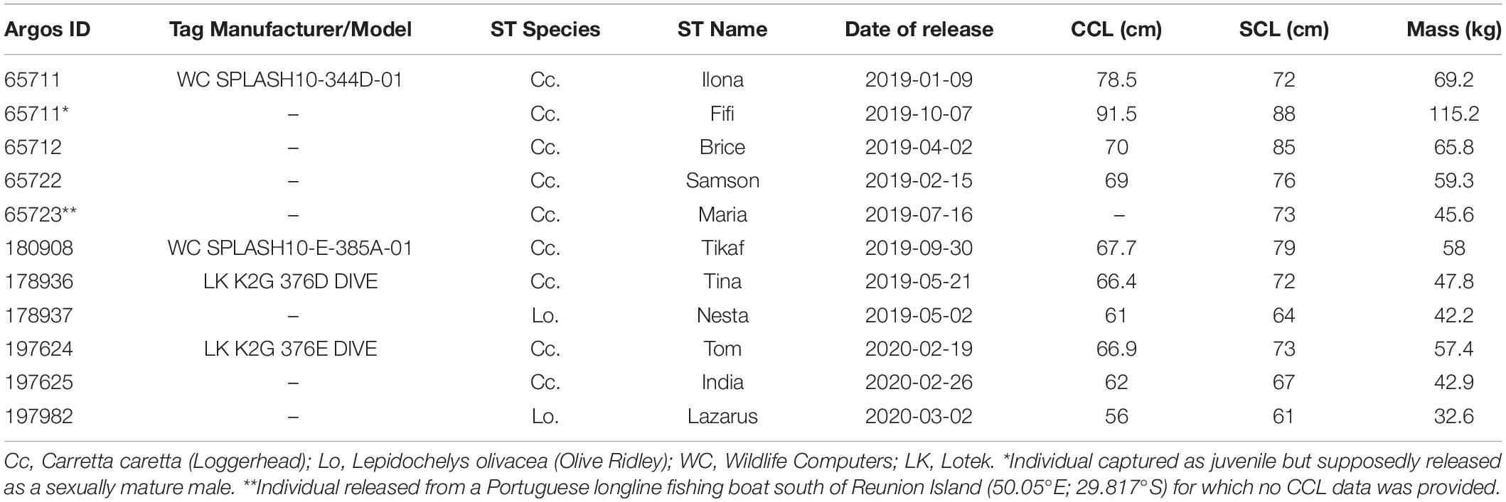
Table 1. ST Morphometrics at release (Standard Carapace Length SCL, Curved Carapace Length CCL, body mass) and tracking parameters (Argos ID, tag manufacturer and model) for the 11 juvenile sea turtles released from Reunion Island (55.28°E; 21.15°S), Indian Ocean.

All animals were considered juveniles, except for the loggerhead called “FIFI,” which was assumed to be a sexually mature male at the time of release. The average individual curved carapace length (CCL) for loggerhead (resp. Olive Ridley) was 70.8 ± 8.9 cm (resp. 58.5 ± 3 cm) and the average weight was 62.35 ± 21.7 kg (resp. 37.4 ± 6 kg). All STs were instrumented at Kelonia and released from Reunion Island, except for the loggerhead ST “MARIA,” which was equipped on board a longliner south of this island (50.05°E; 29.81°S) by a fisheries observer from the Institute of Ocean and Atmosphere (IPMA, Olhão, Portugal). On average, the Kelonia care center rehabilitates and releases ∼25 STs every year. Since the start of the STORM project, in January 2019, about half of the animals released from this center have been equipped with electronic tags recording temperature/depth data.

Sea Turtle Instrumentation and Data Processing

A key element of the STORM program is to ensure that ST handling practices minimize negative effects on animal welfare. As mentioned previously, none of the animal considered in this study was intentionally captured and a particular attention was also dedicated to tag selection. Measurements were obtained from two types of tags (see Table 1), respectively, manufactured by the companies “Wildlife Computer” (WC, 4 × models SPLASH10 and 1 × model SPLASH10-F) and “Lotek” (LK, 5 × model Kiwisat K2G 376). The tags were attached to ST shells using a two-component epoxy resin that is known to pose no threat to the integrity of the animal (Figure 1). Each tag weights ∼200 g, which corresponds to ∼0.3% (resp. 0.5%) of the average body weight of loggerheads (resp. Oliver Ridley) STs considered in this study (international conventions on the preservation of STs allow for the use of tags up to 5% of the animal body weight). Note that one tag (Argos ID 65711) was recovered from the loggerhead “ILONA,” which was poached along the east coast of Madagascar (50.19°E; 15.98°S). This tag was later redeployed on the loggerhead “FIFI” (Table 1) and was thus used twice.

FIGURE 1

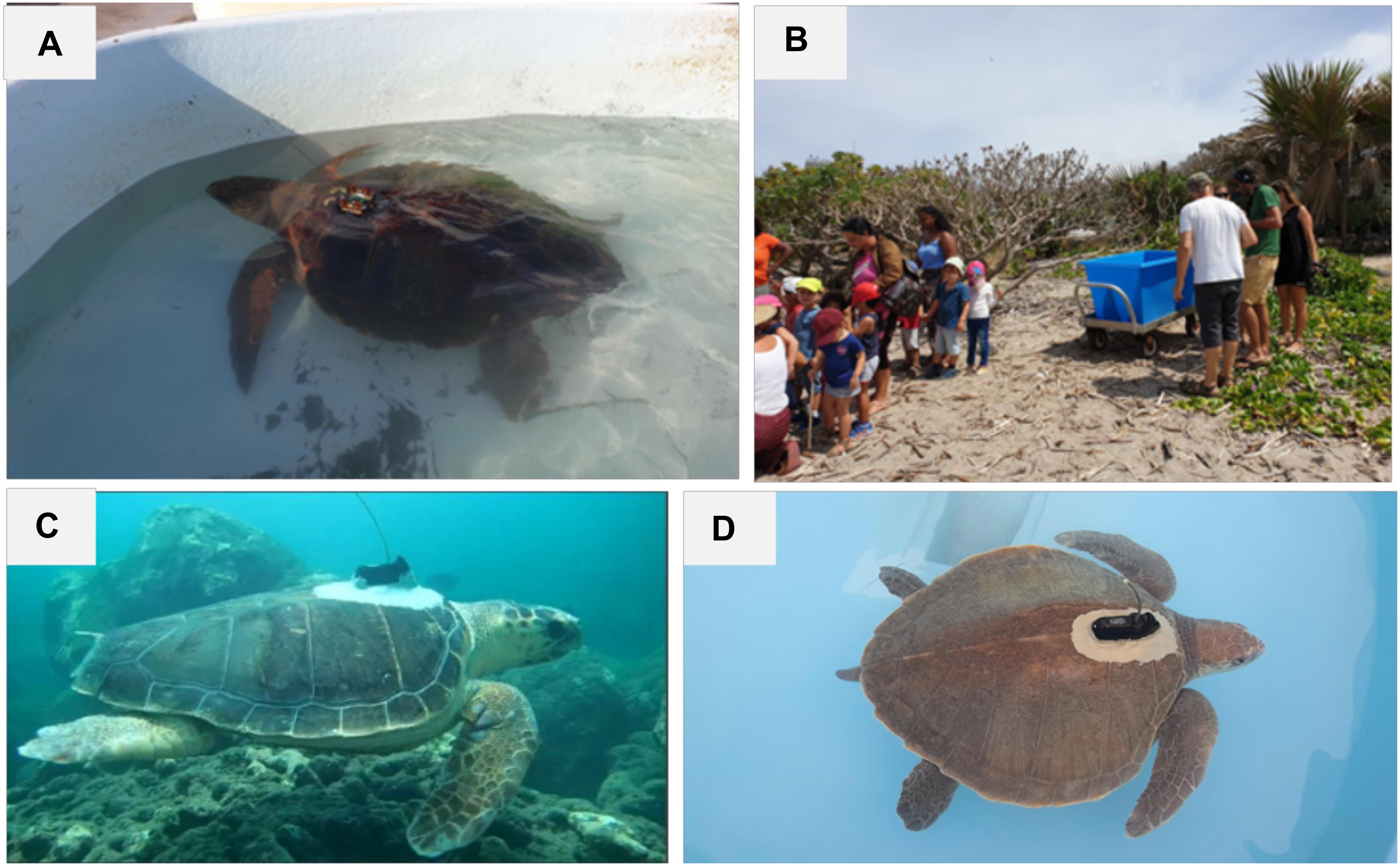
Figure 1. Top panel: Photographs of (A) the loggerhead sea turtle “SAMSON,” which was released in April 2019 after being equipped with a WC SPLASH10 tag. (B) SAMSON release took place in the presence of a primary school class from Reunion Island as part of the outreach program “adopt a turtle.” Bottom panel: loggerhead and Olive Ridley turtles “TOM” (C) and “LAZARE” (D), respectively, released in February and March 2020 after being equipped with LK Kiwisat tags. The underwater photography (D) is extracted from a documentary made by Euronews in February 2020 (https://www.euronews.com/2020/03/30/meet-the- researchers-using-sea-turtles-to-learn-more-about-cyclones).

All tags have been factory calibrated by manufacturers and are given with an accuracy of 0.2° for temperature and 1% for pressure measurement. They were configured to continuously, and simultaneously, sample bivariate time series of external temperature and depth (from pressure) with a time step of 5 min. The repetition rate was set at 15 s for WC tags and 45 s for LK ones. The maximum number of messages per day was set to 500, with priority given to the transmission of time series data. For the one WC tag equipped with Fastloc-GPS technology (WC-SPLASH10-F, Dujon et al., 2014), the sampling interval was set at 1 h with a maximum of four acquisition attempts per hour and high transmission priority. The use of this particular tag was initially intended to evaluate the benefit of Fastloc technology on data sampling (number of collected observations and location accuracy). However, the short life time of this tag (<1 month) did not allow us to conduct this study, which will be carried out during the next phases of the program.

The WC tags were also set to archive all collected depth and temperature measurements every 10 s. The data archive was only recovered from the tag deployed on the poached individual “ILONA” (Argos ID 65711, Table 1). The analysis of this archive allowed to evaluate the effective Argos transmission rate, which was estimated at ∼ one third of collected observations (35%). WC tags were also configured to transmit histograms of maximum depth, dive time, time-at-temperature and time-at-depth, aggregated every 3 h, with medium transmission priority. Examples of information on ST diving behaviour that can be deduced from such data are shown and discussed in the Appendix for STs “BRICE” and “SAMSON”.

Argos location processing was set to use the Kalman filter scheme (Lopez et al., 2013). Collected observations were further processed with the “FoieGras” library (Jonsen et al., 2019) of the R software (R Core Team, 2019) to resample ST trajectories with a regular time step, and to predict ST locations more accurately and at given sampling intervals (5 minutes in the present study). A maximum travel rate of 10 m.s^–1 was used to filter outliers and a minimum time difference of 60 min between observations was used for data to be taken into account in the state-space model.

Spatial and Temporal Distribution of ST-Borne Observations

The number of observations collected by the 11 animals between 9 January 2019 (release date of the first ST “ILONA”) and 30 April 2020 (date of the last measurements transmitted by STs “TINA,” “INDIA,” “TOM,” and “LAZARE” at the time of compiling these statistics¹), is shown in Table 2.

TABLE 2

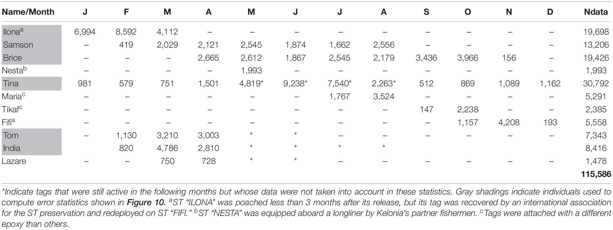
Table 2. Number of temperature observations collected by the 11 STs of the STORM program as of 30 April 2020 indicated by month (JFMAMJJASOND) and by individual (Ndata) with total number shown in bold.

The lifetime of a tag is determined by the capacity of its battery, the charge of which depends on the frequency of transmission, but also by unexpected incidents that may affect the integrity of the tag (or of its attachment material) as well as the animal surfacing behavior itself. According to the parameterized daily allocation for transmission, each tag was expected to transmit for a period of 7–8 months. Including the tags deployed on STs “TINA” and “INDIA,” which are still active 15 and 7 months after being released, respectively, four of the tags did actually transmit for more than 7 months while four have had a duration of less than 3 months (see caption in Table 2 for actual or assumed explanations for the shortened life of these four tags). Overall, the average duration of tags used during this experiment was 5.8 months (6.4 months for LK and 5.2 months for WC) and ranged from 28 days (“NESTA”) to 480 days (“TINA”).

Approximately 115,500 depth-temperature observation pairs (Table 2) were collected during the 16-month period (Jan 2019–Apr 2020) analyzed in this study. As animals were released as soon as they were rehabilitated, no season was particularly favored. Three of the six STs released during the tropical cyclone season (DJFMA) have however been caught in a low-pressure tropical system (STs “TOM” and “INDIA” in TC Herold in March 2020), or in its immediate vicinity (ST “BRICE” in TC Kenneth in April 2019).

The trajectories of the 11 animals equipped in this study are shown in Figure 2A. All STs evolved in an area comprised between 25°N–30°S and 40–65°E, in good agreement with the previous study of Dalleau et al. (2014), which analyzed tracking data of ∼20 loggerhead ST released from Reunion Island during the COCA-LOCA program (Figure 2B). About 70% of the observations were collected in the western part of the SWIO basin (0–30°S; 35–60°E). This region, which concentrates most of the cyclonic activity in the SWIO, is poorly equipped with conventional oceanographic sensors with only four moored buoys (RAMA network) and a dozen ARGO drifters active as of 23 April 2020 (Figure 2B). Many data have also been collected in the northern hemisphere, especially between 10°N–20 °N, by the three individuals (“BRICE,” “SAMSON,” and “TINA”) that managed to reach their breeding area as of 30 April 2020 (ST “INDIA” which was located nearby the equator in late April 2020 (Figure 2A), has also reached the Persian Gulf in June).

FIGURE 2

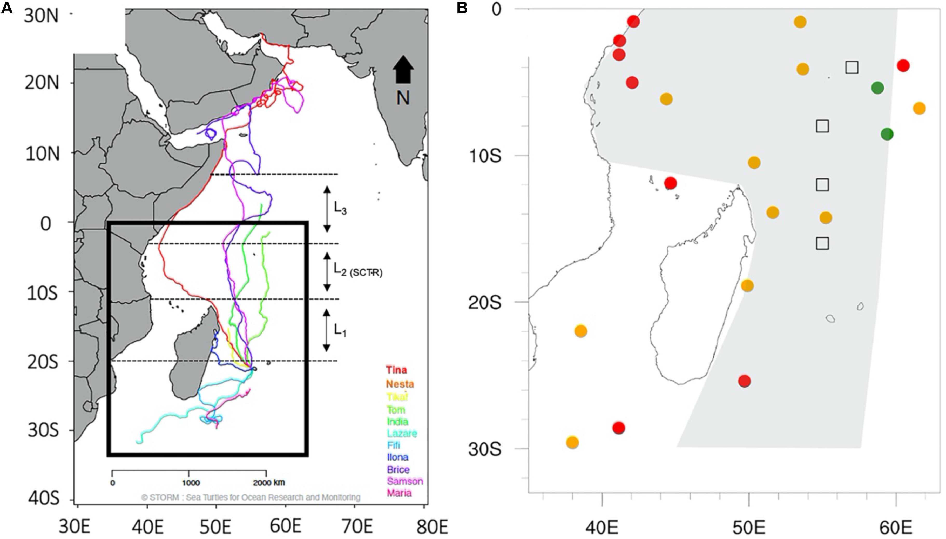
Figure 2. (A) Tracks of the 11 sea turtles equipped between Jan 2019 and March 2020 during the preliminary phase of the STORM project as of 30 April 2020. (B) Location of Argo drifters (circles) and RAMA moored buoys (squares) deployed in the area (35–63°E; 0–33°S) as of 23 April 2020. Green, orange and red colors indicate drifters that have transmitted data in the last 3, 10, and 30+ days, respectively. In (B) the gray shaded area shows the spatial distribution of the 20 loggerhead ST tracked from Reunion island during the COCA-LOCA project (Dalleau et al., 2014). Dashed black lines in (A) show latitude bands LB1 [11°S–20°S], LB2 [3°S–11°S] and LB3 [3°S–7°N] discussed in Figures 5, 11.

The rough analysis of the vertical distribution of ST-borne data (Figure 3) shows that nearly 60% (resp. 40%) of the observations were collected in the first 20 m (resp. in the 20–100 m layer) of the ocean. Below 120 m, data are sporadic (∼1,800, 2%) although temperature measurements have been obtained down to a depth of 320m. Records show a few dive depths up to 400 m (see Figure A1 in the Appendix), but temperature has never been recorded below 320 m. It can also be noticed that ∼60% of the data collected in the first 20 m of the ocean were obtained during the day, but that this proportion is reversed between 20 and 60 m, where 60% of the observations are collected at night (14UTC-02UTC). Below 60 m data appear collected equally during day and night.

FIGURE 3

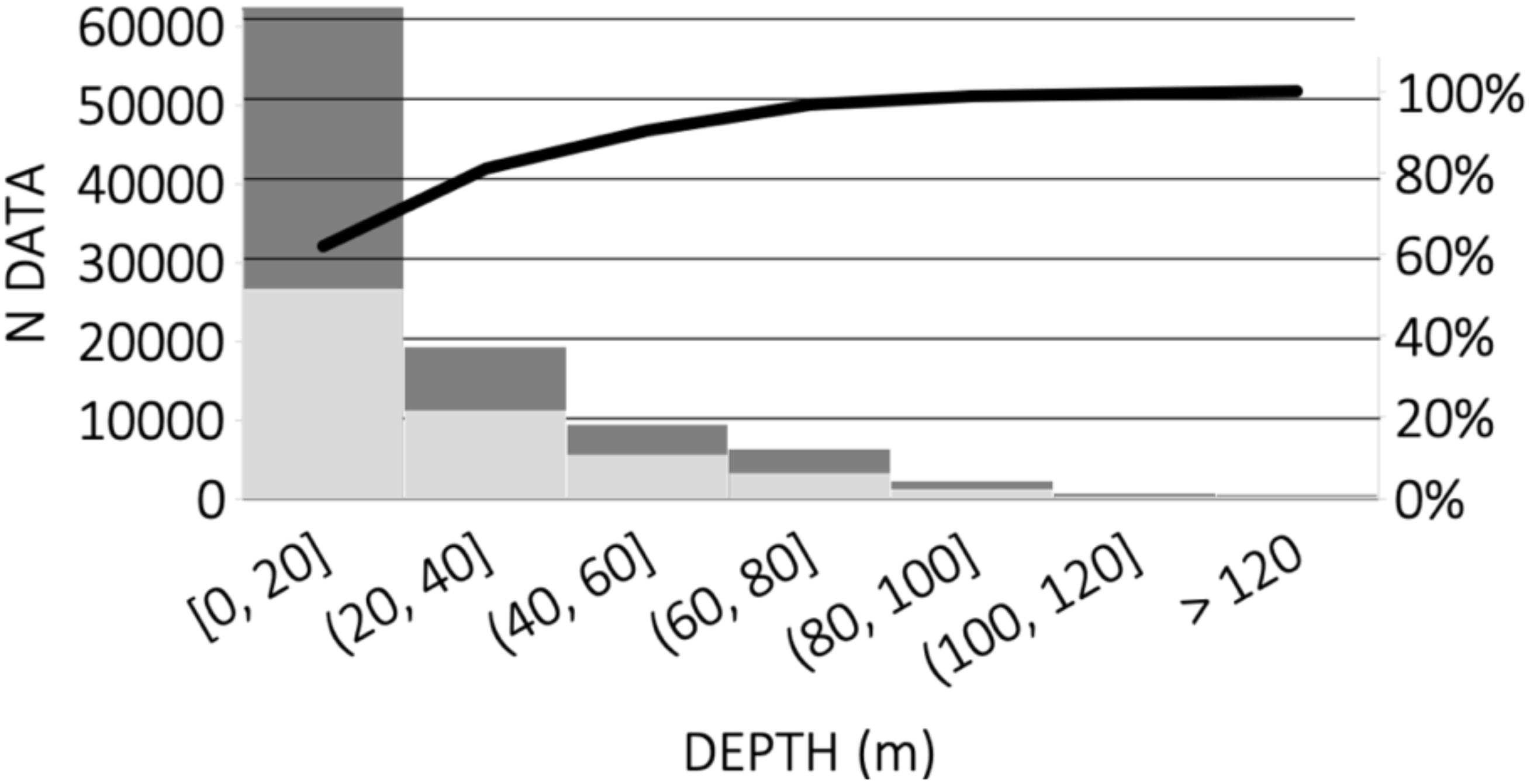
Figure 3. Vertical distribution of data collected by all sea turtles between January 2019 and April 2020. Number of observations (NDATA) between 0 and 120 m in 20 m increments at all times (dark gray) and at night (18–5, Reunion Island Local Standard Time) only (light gray). The black line indicates the cumulative percentage of collected data.

To achieve a more precise description of the vertical distribution of collected ST-borne data, Figure 4 shows the absolute number of temperature observations collected within the first 29 vertical layers of the Glo12 model (0–318 m, see Table 3 for actual model layer depths). Since the vertical levels of the model are not linearly spaced, the density of observations (number.m^–1) within each model layer is also shown in logarithmic scale (black curve). The number of collected data decreases exponentially from ∼29,000 data.m^–1 near the surface to 200 data.m^–1 at ∼11 m depth (model layer # 9) before stabilizing between 11 and 40 m (model layer # 17), and rapidly decreasing again below 100 m (model layer # 22).

FIGURE 4

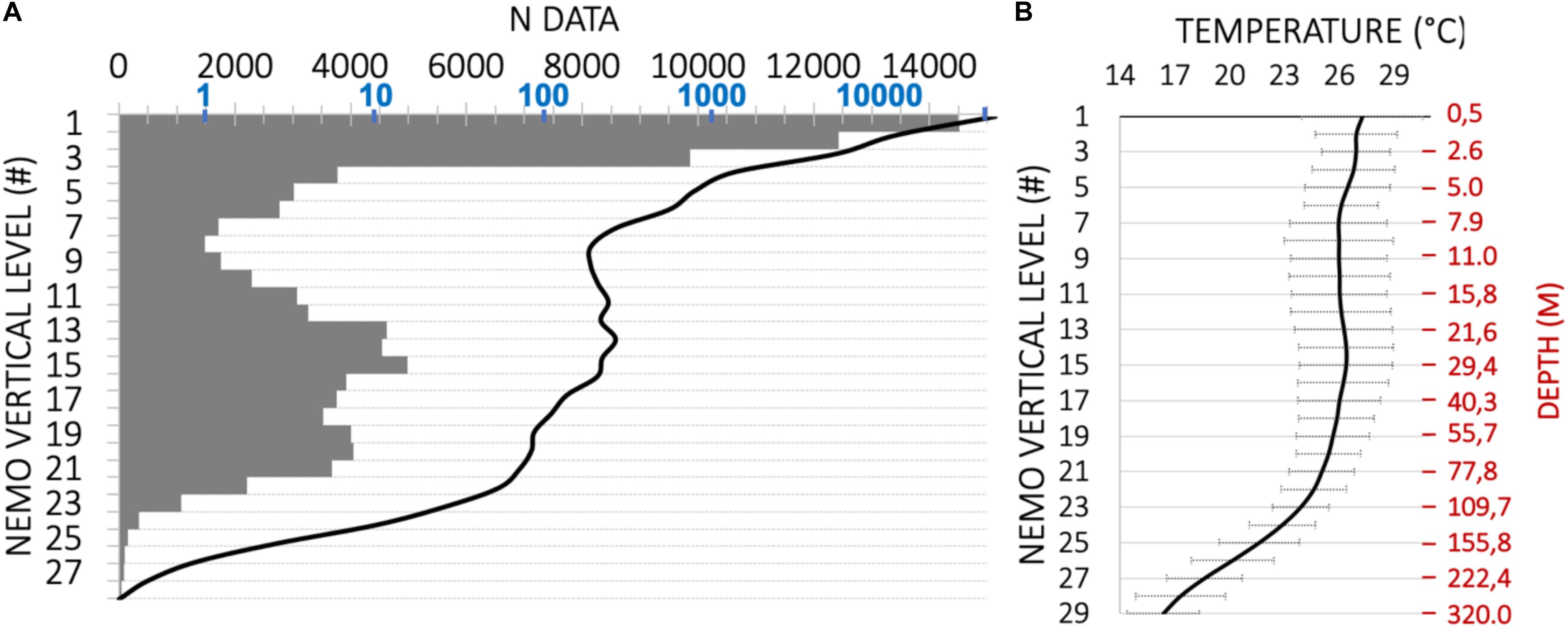
Figure 4. (A) Absolute number of observations collected by sea turtles (NDATA) between January 2019 and April 2020 within the first 29 vertical layers (0–318 m) of Glo12 operational ocean model. The black profile shows the vertical density of the data (number.m^–1, logarithmic scale, max = 29,024) within each layer. (B) Corresponding vertical profile of mean observed temperature with associated std values shown in gray. The corresponding model depths are shown on the right axis (red)—see Table 3 for the actual depth of all model layers.

TABLE 3

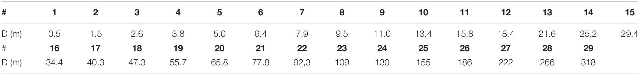
Table 3. Depth (D, bottom of the layer) of Glo12 model levels (#).

Most of the measurements are collected just below the surface (0.5–2.6 m), but a significant number of observations are also gathered between 20 and 90 m, with a secondary peak of ∼5000 data between 30 and 35 m (model layer #16). The associated mean vertical temperature profile (Figure 4B) suggests that these depths correspond to the lower half of the mixed layer, whose bottom varies between 25 and 40 m in the sampled region, depending on geographical areas (cf. Figure 5). This layer is therefore a rather attractive area for STs, possibly for foraging (due to nutrient injection from colder waters below) and/or because these depths correspond to their neutral buoyancy. The strong temperature gradient observed near 100 m depth also matches a clear break in the data density profile, suggesting that STs prefer to evolve in waters warmer than 23°C. The depth of 320 m also seems to represent a strong physiological barrier for the animals (Narazaki et al., 2015) although (very) few dives have been recorded down to almost 400 m (see Appendix).

FIGURE 5

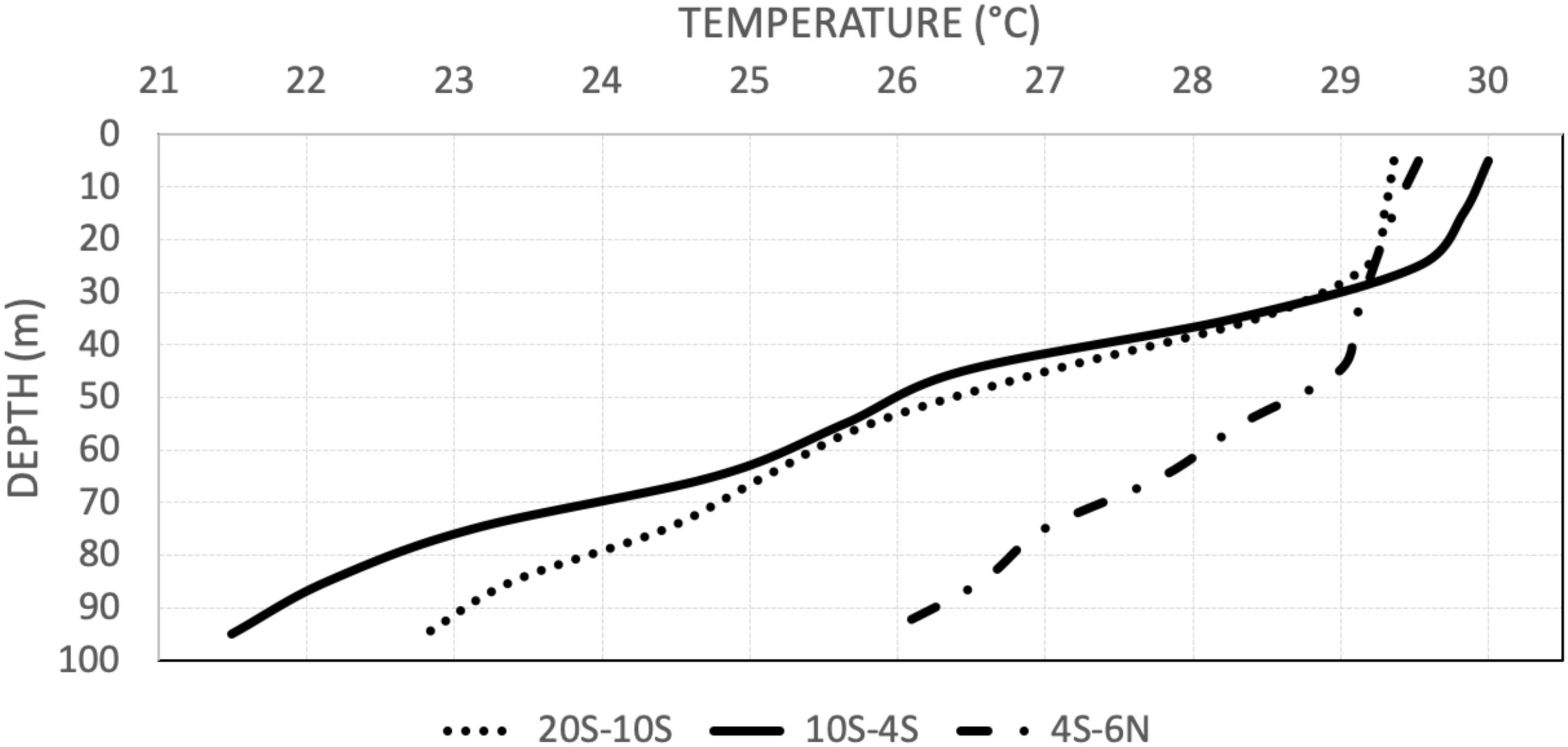
Figure 5. Mean vertical profiles of ocean temperatures in 10 m steps, as deduced from data collected by ST SAMSON (10/02–29/04 2019) and BRICE (7/04–10/07 2019) within latitude bands LB1 [20°S–11°S] (dash), LB2 [11°S–3°S] (plain) and LB3 [3°S–7°N] (long dash) shown in Figure 2.

Evaluation of Sea Turtle Temperature Measurements

Example of Average Vertical Temperature Profiles

In order to qualitatively assess the realism of temperature structures sampled by STs, Figure 5 presents mean temperature profiles derived from the analysis of the data collected by the ST “SAMSON” and “BRICE” between 20°S and 6°N (∼3,000 km). These two animals, released about 2 months apart, followed a similar trajectory (Figure 2A), except between the equator and 5°N, where strong currents forced the individual “BRICE” to change its course. Approximately ∼2½ months were required for individual “SAMSON” to travel the 3,000 km from Reunion to the Gulf of Oman, compared to just over 3 months for ST “BRICE” (which was also delayed by Tropical Cyclone Kenneth near 10°S in April 2019). To account for the spatial variability of ocean temperatures, and to ensure a relative temporal continuity, the vertical profiles shown in Figure 5 were computed in the three distinct latitudinal bands shown in Figure 2: 21°S–10°S, 11°S–3°S and 3°S–7°N (hereafter referred to as LB1, LB2 and LB3, respectively).

Observed temperatures near the surface appear relatively uniform across the whole transect, with mean values comprised between 29.2 and 30°C in the first 20 m. SST is also relatively uniform, although slightly higher (30°C) in the SCTR area (LB2) than in the other two regions (∼29.5°C). Below 20 m, significant regional differences can be seen in the vertical structure of ocean temperature. First of all, the mixed layer depth (MLD), identified by a strong gradient in vertical temperature profiles, varies significantly with latitude. It averages at ∼25 m in the southern hemisphere (27 m in LB1 and 22 m in LB2), but deepens to 40 m in the trans-equatorial area (LB3). The rate of temperature decrease in the OML is fairly uniform in the three regions, but also changes subsequently underneath. It is thus relatively slow in the LB3 zone, with a temperature of 26°C at 100 m depth (∼−5°C/100 m), but increases significantly in the two northernmost areas to reach ∼−8.5°C/100 m in LB1 (22.8°C at 100 m depth) and ∼−11°C/100 m in LB2 (21.5°C at 100 m depth). The differences on either side of the SCTR (LB2) are expected and reflect the existence of strong upwelling and a shallow thermocline in the SCTR region (Hermes and Reason, 2008, 2009). The potential capability of sea turtles to capture the spatial variability of the mixed layer and thermocline, which has important impacts on the Indian summer monsoon (Annamalai et al., 2005) and tropical cyclone activity (Xie et al., 2002) in this part of the world, is particularly encouraging.

Comparison With ARGO Drifter Data

In order to quantitatively evaluate the temperature measurements provided by STs, a comparison with ARGO profiler data, whose quality is well-established, can be particularly instructive. As shown in the previous section, however, the limited spatial and temporal resolution of the ARGO profiling network within the area of evolution of ST considered in this project (see Figure 2B) makes direct comparisons with ARGO temperature data difficult. Hence, we could only find four opportunities for such comparisons during the first 16 months of the STORM program (Figure 6, see caption for details on locations, dates and procedures for temperature profile comparisons): in June 2019 for individual “TINA” (Figures 6A, position/time difference of ∼33 km/15 days), in April 2019 for individual “BRICE” (Figure 6B, position/time difference of ∼124 km/3 days), in March 2019 for individual “SAMSON” (Figure 6C, position/time difference of ∼68 km/2 days) and in April 2020 for individual “INDIA” (Figure 6D, position/time difference of ∼73 km/6 days).

FIGURE 6

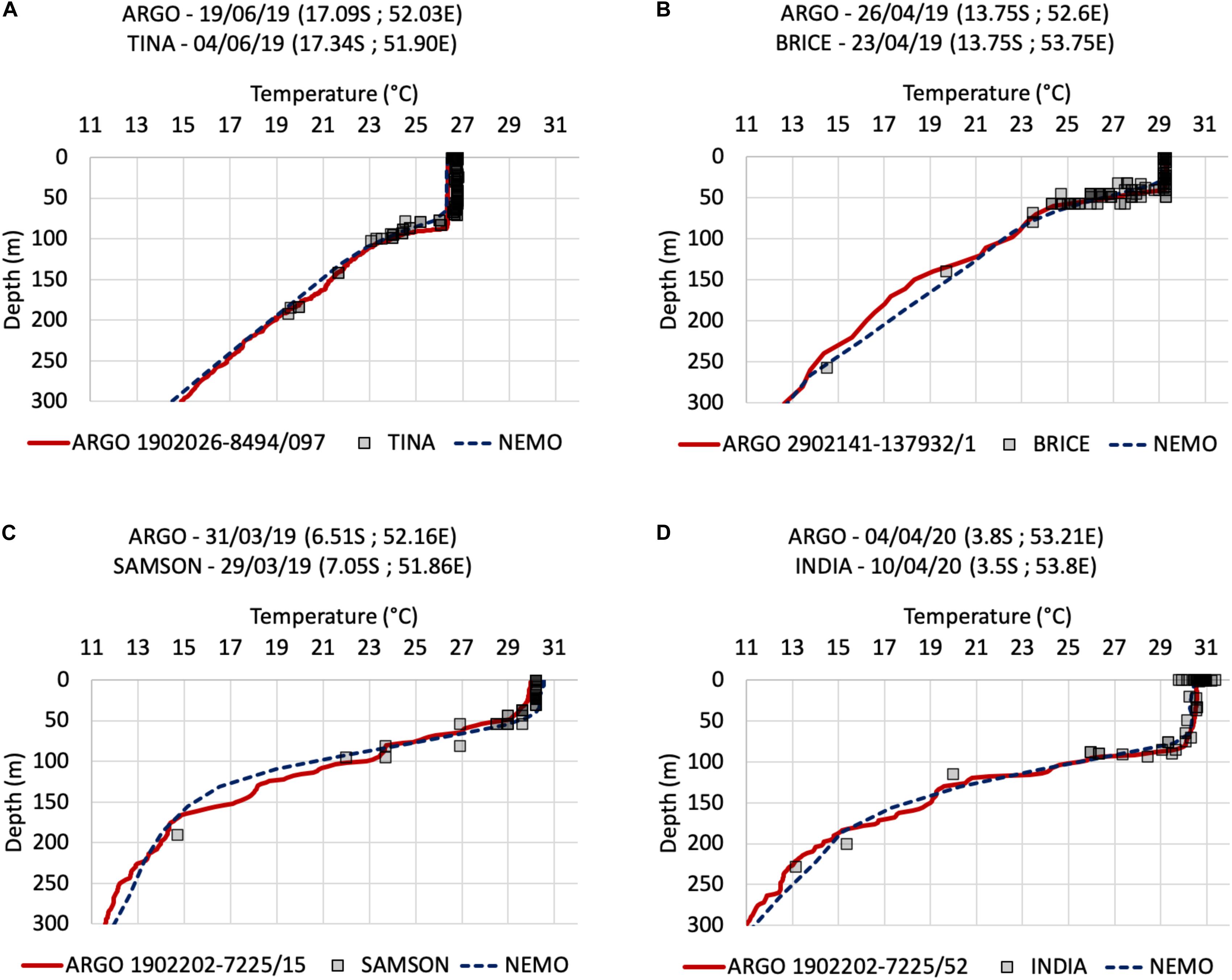
Figure 6. Comparison of various ST-borne (square), ARGO (red) and Glo12 (blue dotted) temperature profiles in the SWIO basin on (A) 19 June 2019, (B) 26 April 2019, (C) 31 March 2019 and (D) 4 April 2020 (see details at the top and bottom of each sub-panel for information on the date, reference and location of the profiles). Temperature profiles derived from ARGO and Glo12 are both spatially and temporally localized, while ST profiles consist of aggregated temperature measurements over a 12–18-h period at the nearest ARGO positions within a 3–14-day interval.

Given the limited spatial and temporal variability of tropical oceans under normal conditions (i.e., in the absence of tropical cyclone) over distances (resp. periods) of a few tens of km (resp. days), imperfect collocation of ARGO/ST observations is expected to have limited impact on temperature data comparisons. Thus, it can be seen that ST and ARGO temperature measurements are generally in good agreement at the four considered times/locations. Small discrepancies can nevertheless be observed in the first 50–60 m of the ocean in the SCTR region (Figure 6C), possibly due to a strong oceanic response to atmospheric forcing during the period considered. A 1.5°C variability in ST-borne measured SST is also observed in the intertropical zone (Figure 6D), which may partly reflect the diurnal cycle of SST, estimated at 0.5–1.5 K in the tropics by Yang and Slingo (2001).

Comparison With Satellite SST Measurements

Another possibility to assess the accuracy of SST temperature observations is to compare ST-borne observations with spaceborne measurements.

Current SST observations rely primarily on the use of radiometric sensors deployed on board scrolling (e.g., METOPs) or geostationary (e.g., MSG) Earth observation satellites. These data generally consist of a combination of observations collected by radiometric sensors operating in the thermal infrared and/or microwave range—infrared sensors are more accurate than microwave sounders but are very sensitive to the presence of clouds. To date, there are a dozen operational satellite SST products available to the research community with spatial resolutions ranging from 0.01° to 0.5°. In the following, ST-borne SST data collected at or just below the sea surface are compared to three sets of subskin satellite SST products : (i) the low-resolution (0.25°) OSTIA (Operational Sea Surface Temperature and Ice Analysis) dataset, operationally produced by the United Kingdom Met-Office, and (ii) two versions of the high-resolution (0.05°) OSI-SAF (Satellite Application Facility on Ocean and Sea Ice) dataset, produced by the French Meteorological Service Météo-France.

The level 4 OSTIA diurnal SST product is based on the United Kingdom Met Office system (Donlon et al., 2012) and distributed by CMEMS². It contains global hourly mean SST data at 0.25°× 0.25° horizontal resolution derived from in-situ and space-borne infra-red radiometer observations. It uses radiometric data collected by more than 10 satellites (e.g., MSG, GOES, MetOp-A) provided by the Group for High-Resolution Sea Surface Temperature (GHRSST, Martin et al., 2012).

OSI-SAF products used in this study are distributed by the EUMETCAST Data Centre³ and are available at a space-time resolution of 0.05°× 0.05°/1 h. OSI-206-a is an operational product, released in February 2018, which provides SST data over the Atlantic and Western Indian Oceans (60 S–60 N; 60 W–60 E) from the SEVIRI imager on the Meteosat second generation (MSG-) 11 satellite at 0° longitude (OSI/SAF, 2018b). OSI-IO-SST is a demonstration product released in March 2017 that provides SST data over the Indian Ocean (60 S–60 N, 19.5 W–101.5 E), derived from MSG-8 measurements at 41.5° longitude (OSI/SAF, 2018a). These two datasets are therefore based on independent observations, but use similar inversion methods. All three products have a target accuracy of 0.5°C (Std of 1°C).

In the following, all in-situ data collected between the surface and 51 cm depth (to be consistent with the analysis presented in the next section) are considered as SST observations. In order to discard potentially erroneous satellite observations due to imperfect atmospheric corrections in coastal areas (Brewin et al., 2017), ST-borne and satellite SSTs collected within 30 km of the coast are excluded from this analysis. After application of this land-sea mask, the ST dataset contains 38,900 data for OSTIA and 37,940 data for OSI-SAF, respectively. The results of these comparisons are shown in Figure 7.

FIGURE 7

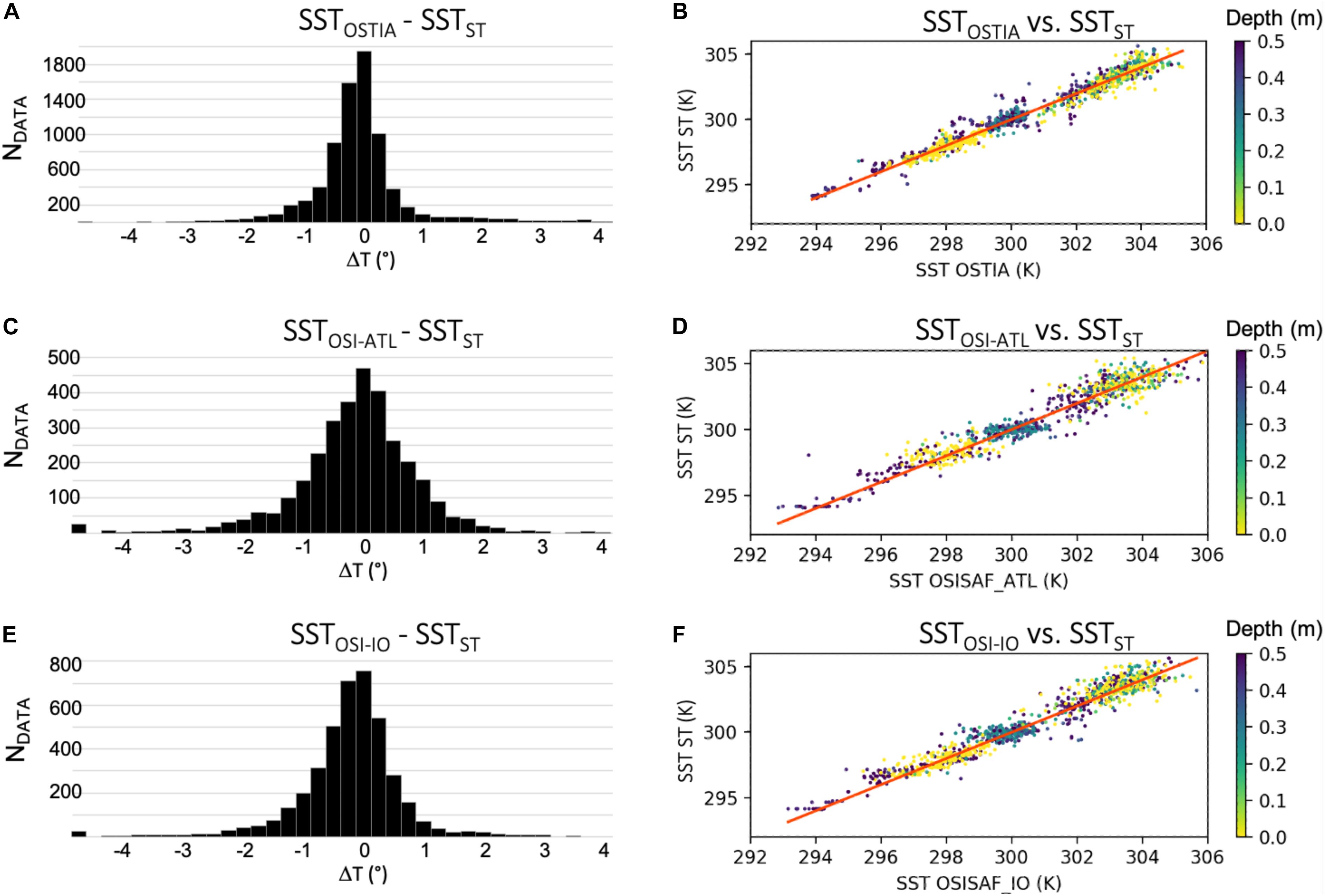
Figure 7. Histogram (left panel) and scatterplot (right panel) of differences between SST data collected by STs (SST_ST) and inferred from the satellite products: (A,B) OSTIA (SST_OSTIA), (C,D) OSI-SAF 206a (SST_OSI–ATL), and (E,F) OSI-SAF IO (SST_OSI–IO), between January 2019–April 2020. Colors in subpanels (B,D) and f indicate the depth of collected ST measurements between 0 and 0.51 m (color scale to the right). The red line in (A–D) corresponds to the 1:1 line.

Overall, SST data collected by ST vary between 20° and 32°C throughout the domain. Error statistics show that SST satellite data are, on the whole, very close to the ST-borne measurements although a slight systematic underestimation can be noticed for each of these three products with respect to ST data.

The comparison of ST-borne SST measurement against OSI-SAF operational (Figures 7C,D, OSI-ATL) and demonstration (Figures 7E,F, OSI-IO) products gives similar results, with a bias of ∼−0.12°C (Std 0.59°C) for OSI-IO compared to −0.06°C (Std 0.72°C) for OSI-ATL. The errors follow a Gaussian distribution for both products, but the distribution appears slightly biased toward negative values for OSI-IO (Figure 7E). The dispersion, which remains relatively uniform across all temperature ranges, is however slightly lower for the demonstration product (Figure 7F) than for the operational one (Figure 7D). For the OSTIA dataset (Figure 7A), the errors also follow a normal distribution (bias/std of ∼−0.05°/0.52°). The magnitude of the errors is slightly smaller than that of the OSI-SAF products, probably due to the lower resolution of this dataset (0.25° vs. 0.05°). The dispersion (Figure 7B) is also rather low and, again, generally uniform across all temperature ranges.

These values are in good agreement with the maximum margin of error expected for both ST-borne (0.2°) and satellite (0.5°± 1°) measurements, which attests to the good accuracy of both in situ and remotely sensed measurements in the area of evolution of STs. It should also be noted that considering ST data collected precisely at or slightly below the ocean surface (i.e., down to 0.51 m) does not affect comparisons with satellite subskin SST data. The dispersion thus remains the same regardless of the depth of the ST measurements (see colors in Figures 7B,D,F).

Evaluation of Glo12 Temperature Forecasts in the Western Tropical Indian Ocean

Model Data

In this Section, ST-borne data are used to evaluate temperature forecasts from Mercator-Ocean 1/12° global operational model Glo12, based on the Nucleus for European Modeling of the Ocean (NEMO) OGCM. NEMO is a state-of-the-art community modeling framework for research and forecasting in ocean and climate science, developed by a European consortium (Madec et al., 2019). The Glo12 forecast model version 3 is based on version 3.1 of NEMO and is notably used by Mercator-Ocean to provide ocean forecast products to CMEMS as part of the European Earth observation program Copernicus. It uses an ORCA grid type of 1/12° (∼0.08°), with 50 vertical levels whose resolution decreases from 0.51 m at the surface to 450 m at the bottom (see Table 3 for the depth of Glo12 first 29 levels). In the tropics, Glo12 assimilates satellite altimetry and SST observations, such as the OSTIA product presented in section “Example of Average Vertical Temperature Profiles,” as well as in situ observations such as ARGO, mooring buoy data and vessel-based observations, among others. More details on this model can be found in Lellouche et al. (2018). The Glo12 temperature data used in this study are available on an hourly basis for SST and every 6 h for all other depth levels⁴.

Assessment of Modeled SST

Comparisons between ST-borne SST data and Glo12 forecasts over the 16-month analysis period are shown in Figure 8. This analysis uses all data collected between the surface and 51 cm (corresponding to the bottom of the first model layer) over the period January 9, 2019 to April 23, 2020. In-situ temperature observations are interpolated to the model grid and averaged over a period of ±30 min around the round hour in each grid cell of the model.

FIGURE 8

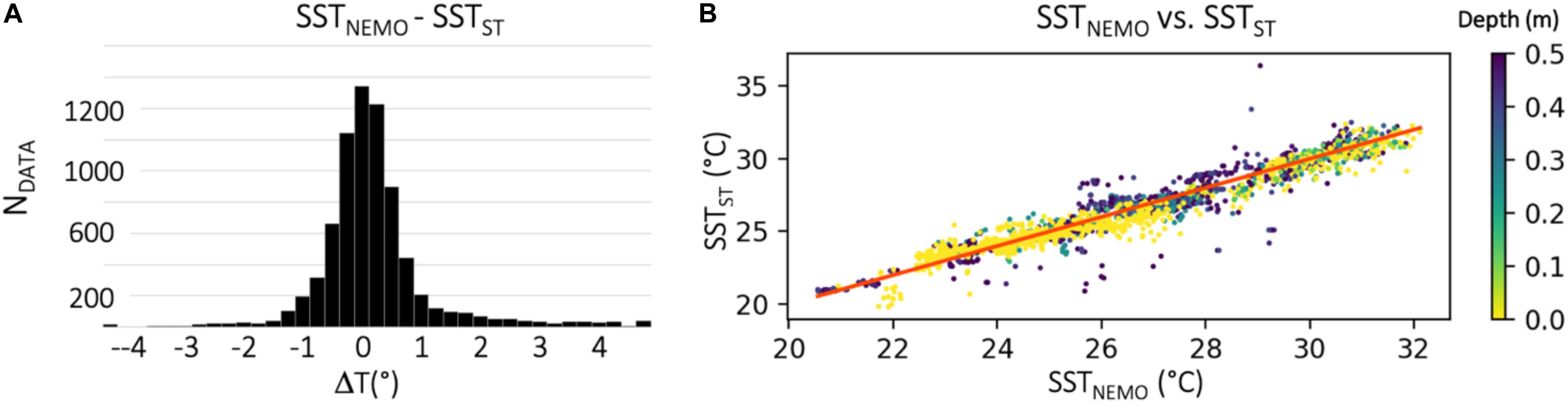
Figure 8. As in Figure 7, but for (A) Histogram and (B) scatterplot of differences between SST collected by STs (SST_ST) and forecasted with Glo12 (SST_NEMO).

The comparison between in-situ and modeled SST shows good agreement over the domain and period of analysis considered. The resulting bias (0.09°C) and standard deviation (0.67°C) errors are quite small and the dispersion is relatively uniform (Figure 8B), except in the range 24–28°C where it appears to be slightly larger. The error distribution follows a centered Gaussian distribution (Figure 8A) slightly biased toward positive values (higher model temperatures compared to ST measurements). Such an agreement is not surprising since OSTIA SST data are assimilated in the Glo12 model to constrain model temperatures at the surface (Gasparin et al., 2018). As we will see later, forecasts of subsurface temperature, where no satellite data and few in-situ observations are available, however show larger errors.

Evaluation of In-Depth Modeled Temperatures

Figure 9 shows comparisons between ST-borne temperature observations and Glo12 forecasts at depths comprised between 0 and 320 m. In-situ data are interpolated to the model grid and averaged over a period of ±3 h, every 6 h and within each grid cell.

FIGURE 9

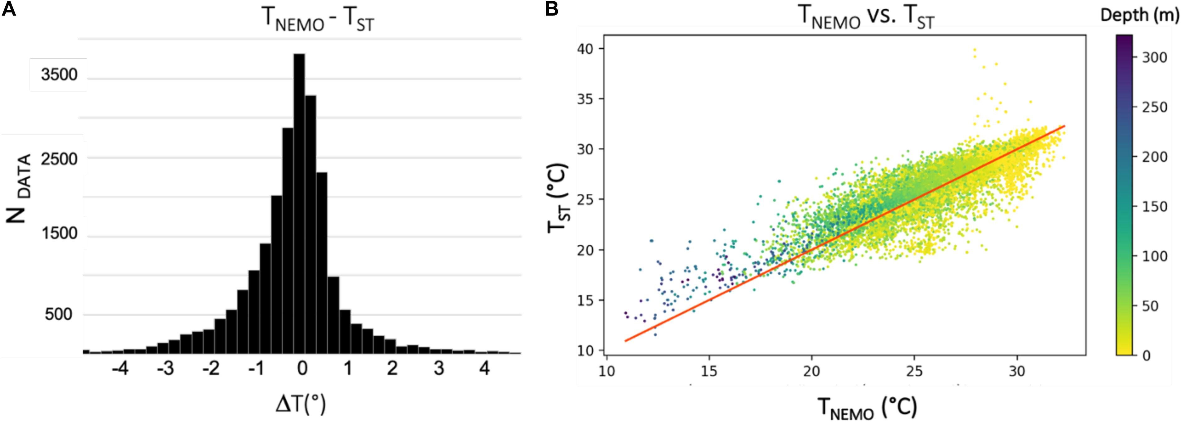
Figure 9. As in Figure 7, but for (A) Histogram and (B) scatterplot of differences between Glo12 (TN_EMO) and ST (T_ST) temperature between 0 and 320 m depth.

Overall, the dispersion (Figure 9B) is greater than that observed for SST (Figure 8B). With the exception of the lowest temperatures (<20°C), it is nevertheless relatively uniform and evenly distributed on both sides of the 1:1 line. However, the sign of temperature differences varies significantly with depth. Within the first 25 m (yellow dots in Figure 9B), the model tends to overestimate ocean temperatures, with maximum differences being observed for temperatures in the 25–30°C interval. From a depth of 50 m (green color), this trend reverses and suggests an underestimation of model temperatures compared to in-situ observations, which grows as depth increases (>150 m, blue color). This trend is also found in the distribution of temperature differences (Figure 9A), which shows a Gaussian distribution biased toward negative values.

Figure 10A provides additional insight into the performance of Glo12 in-depth temperature forecasts in the tropical Indian Ocean. In this analysis, data collected within the area [20°S–15°N] (see ST considered in Table 2) are compared to Glo12 temperature predictions for the first 26 levels of the model [the limited amount of ST data available below 155 m (red curve in Figure 10A) does not allow to extend this comparison to lower model levels].

FIGURE 10

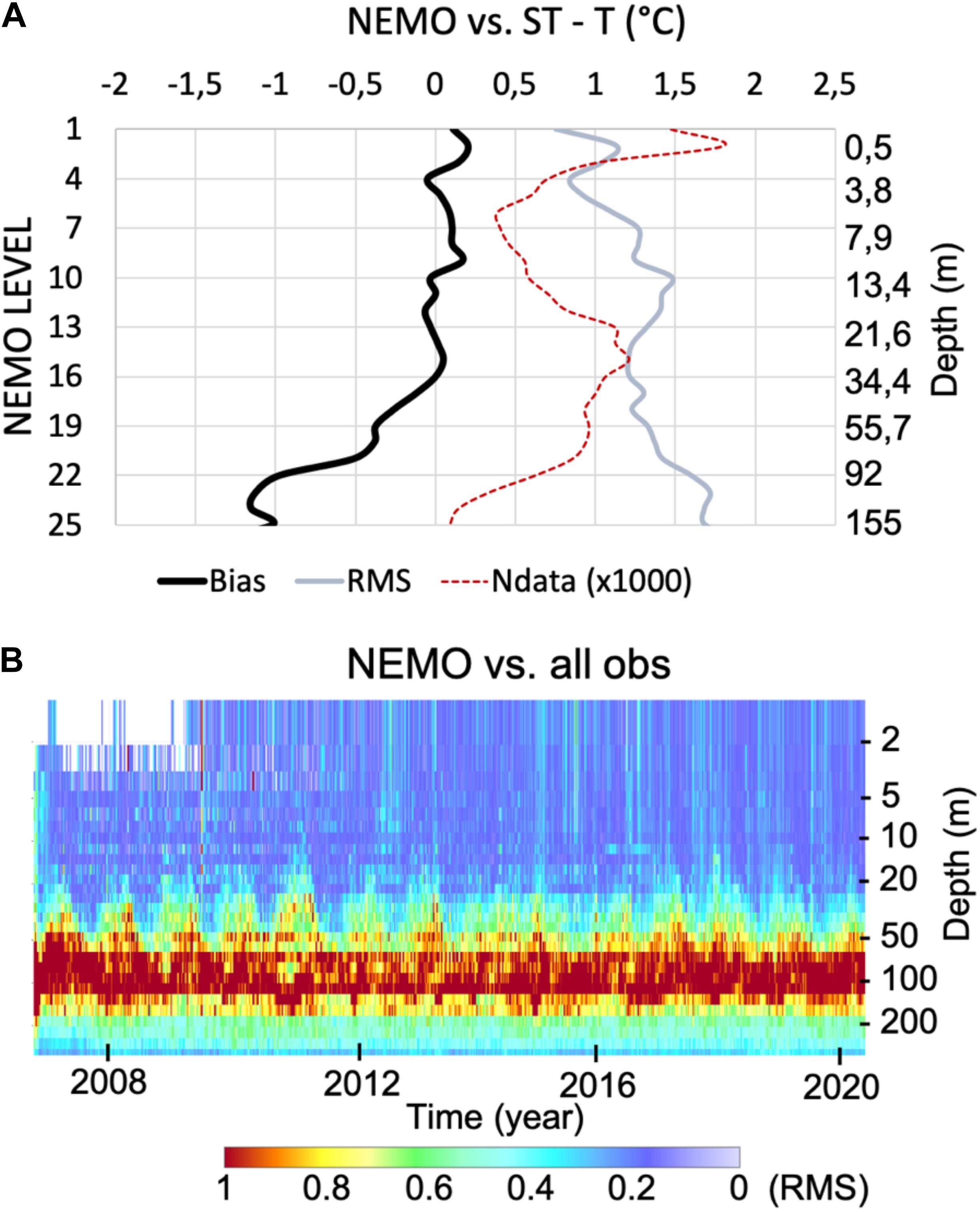
Figure 10. (A) bias (black curve) and RMS (gray curve) errors between Glo12 temperature forecasts and ST-observations as a function of model level (left axis)/depth (right axis) in the W tropical Indian Ocean (20°S–15°N; 40°E–60°E). The red curve indicates the number of model grid points considered in the analysis at each level (x-axis × 1,000). (B) Time series of operational RMS error estimates against all available in-situ temperature observations in the tropical Indian ocean (30°S–30°N; 40°E–120°E).

Analysis of the vertical profile of the mean bias error [T_NEMO–T_ST, black curve)] shows excellent agreement within the first 35 m (16 first model layers). Within this layer, which more or less corresponds to the depth of the OML in this area (Figure 5), the bias is close to zero. Below 35 m, it does however increase rapidly to reach nearly −1.2° at a depth of 155 m. The associated root mean square (RMS) error (gray curve) also tends to increase more or less linearly with depth, from 0.7°C at the surface to 1.6° at 155 m.

These results are qualitatively consistent with Glo12 forecast verification scores performed since 2008 in the tropical Indian Ocean. As shown in Figure 10B, the comparison of Glo12 temperature forecasts against conventional in-situ observations (ARGO, RAMA, drifting surface buoys, ship measurements) hence shows a systematic increase of the RMS error starting from 30 m downwards. The error is maximized near 100 m before decreasing rapidly beyond 140 m. The vertical distribution of the RMS error is probably related to an excessive diffusion of the model, which prevent it from keeping the thermocline, and associated temperature gradients, at the correct depth (∼100 m on average at the basin scale). Once past the thermocline, the temperature variation is, however, significantly reduced, mitigating the impact of the diffusion. From a quantitative standpoint, one can note that the RMS error computed from ST observations (Figure 10A) is higher than that estimated from conventional in-situ data. Such difference can be possibly explained by the sizes of the comparison domains [(20°S–15°N; 40–60°E) in Figure 10A vs. (30°S–30°N; 40–120°E) in Figure 10B] as well as from the higher space-time distribution (and number) of ST observations.

This overall tendency nevertheless shows significant variability when areas and time periods are considered independently. As shown in Figure 7, the comparisons of Glo12 temperature forecast against ARGO and ST observations show different model performance depending on the location/period considered. In order to further investigate this issue, Figure 11 shows comparisons (scatterplots) of temperature data collected by STs “SAMSON” and “BRICE” and predicted by Glo12 in the latitude bands (7°N–3°S) (LB1), (3°S–11°S) (LB2), and (11°S–20°S) (LB3), already considered in Figure 5. As mentioned above, these two individuals, released at about 2-month intervals, followed an almost identical trajectory between Reunion Island and 5°N (Figure 2). In each of the three geographical areas considered, ST observations were collected over periods of 4–6 weeks, separated by about one and a half months.

FIGURE 11

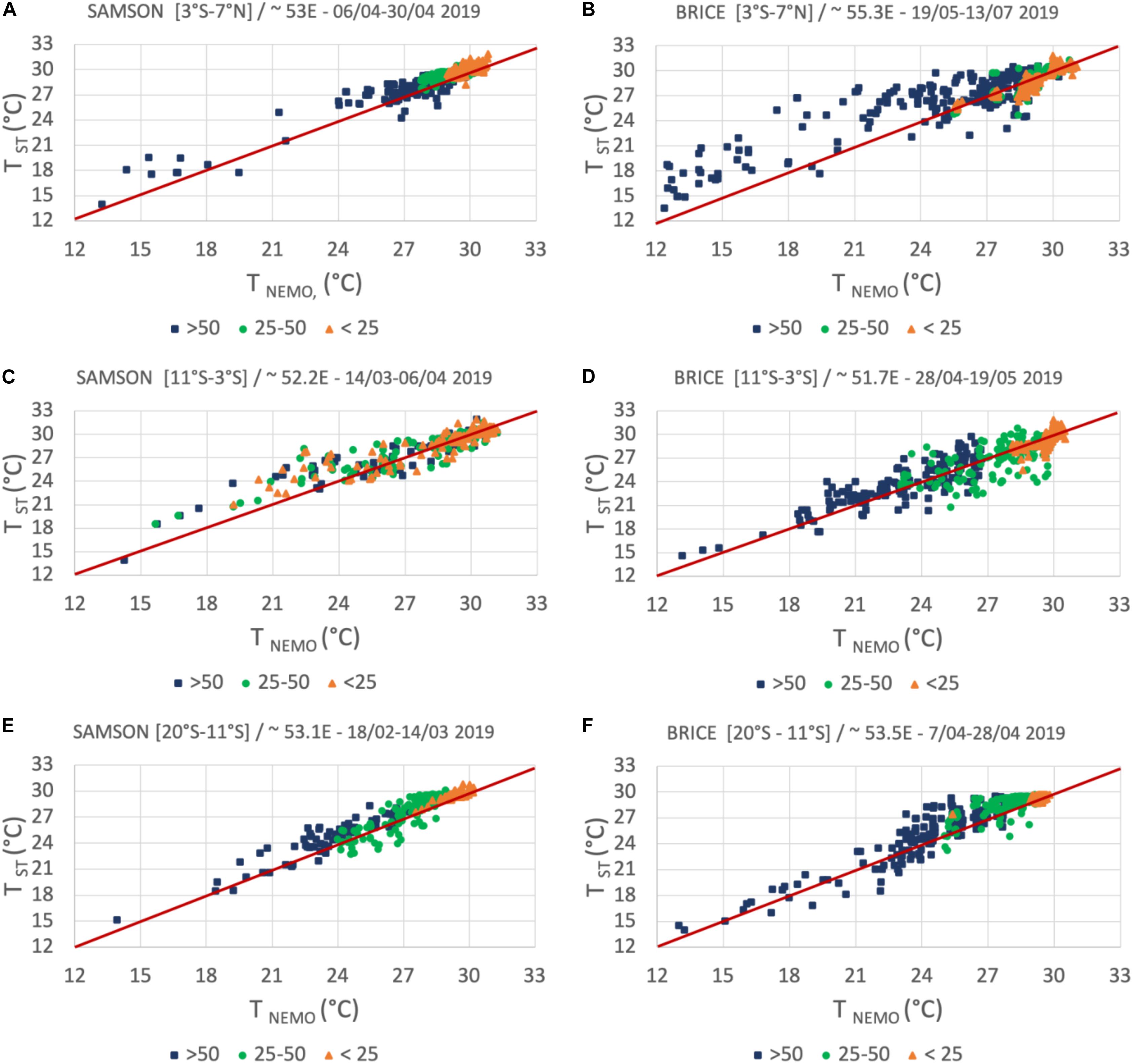
Figure 11. Scatterplots of temperature data collected by STs (T_ST) SAMSON (left panel) and BRICE (right panel) and forecasted by Glo12 (T_NEMO) within latitude bands (A,B) (3°S–7°N), (C,D) (3°S–11°S), and (E,F) (11°S–20°S) shown in Figure 2. The associated mean longitude and comparison period are given on top of each panel.

The data collected by the individual “SAMSON” were obtained during the second half of the summer season (mid-February–end of April). Overall, one notes a systematic underestimation of model predicted temperatures in the three geographical areas, which tends to become more pronounced as depth increases [mean differences between models and observations of −0.27°/−0.4° and −0.5° in LB1 (Figure 11A) for D1 (<25 m), D2 (25–50 m), and D3 (>50 m), respectively; −0.1° (D1)/−0.13° (D2) and −0.5° (D3) in LB2 (Figure 11C); −0.12° (D1)/−0.3° (D2) and −0.8° (D3) in LB3 (Figure 11E)]. Comparisons made in these same areas from data collected by ST “BRICE” toward the end/beginning of the summer/autumn seasons (mid-April–mid-July) nevertheless show different results. In the trans-equatorial zone (LB1, Figure 11B), Glo12 tends to overestimate ocean temperatures above 50 m [(+0.24° (D1)/+0.28° (D2)], but shows a significant underestimation below 50 m (−1.1°). This tendency is also observed in the SCTR region (LB2, Figure 11D) with mean differences between model and observations of +0.2° (D1)/+0.5° (D2) and −0.5° (D3). In the southernmost region (LB3, Figure 11F) these figures are, however, similar to those obtained in summer [+0.2° (D1)/+0.5° (D2) and –0.7° (D3)].

Although the amount of data used in this analysis is clearly not sufficient to draw strong conclusions on the performance of Glo12 at the regional and seasonal scales, these results suggest a strong seasonal and spatial dependence of the model performance, especially in the first 50 m of the ocean. In contrast, the model’s tendency to significantly underestimate ocean temperatures below 50 m appears systematic and is broadly consistent with the global figures presented in Figure 10.

Conclusions, Discussion and Perspectives

The exploratory measurements collected during the first phase of the STORM project (January 2019–June 2020) aimed to assess the capabilities of ST’s equipped with environmental tags to sample the thermal properties of the western tropical Indian Ocean. Although based on a limited dataset (11 sea turtles, ∼115,000 observations), the preliminary results obtained during this experiment confirms the quality of temperature observations provided by ST and clearly shows potential for ocean monitoring and forecasting in this tropical area. Comparisons of temperature profiles collected by STs with measurements from co-located ARGO drifting buoys are in good agreement at all sampling depths (0–250 m), while comparisons with various SST satellite products fall within the expected uncertainties with a slight overestimation of ST-derived temperature data of ∼0.2° ± 1°. The comparison of ST-borne surface and subsurface temperature observations with Glo12 ocean model forecasts also demonstrated the potential of such in-situ data to assess the performance of ocean models in this relatively poorly instrumented area. Although more consistent datasets are needed to implement a robust, long-term, verification strategy, ST data collected in 2019 and 2020 have shown the good performance of GLO12 surface and subsurface (<50 m) temperature forecasts, with a mean bias error (resp. RMS) between −0.5°C and +0.5°C (resp. 0–1.5°C). A potentially large spatial and seasonal variability is also suggested and will be studied in more detail in the future. At lower depths, the model is also shown to significantly underestimates ocean temperatures, as already observed from global operational assessments carried out at basin scale.

A particularly striking result of this study is related to the ability of ST to collect large amount of data in the upper 100 m of the ocean, a depth that more or less correspond to the maximum depth of the mixed layer in tropical oceans (Chu and Fan, 2010). By separating the atmosphere from the deep ocean, the mixed layer modulates the exchange of energy and mass between these two environments (Dong et al., 2008). A better knowledge of these exchanges is key to further understand the processes that drive the life cycle of low-pressure tropical weather systems as well as the impacts of climate events on the marine ecosystem. The possibility of using ST-borne observations to identify the thickness of the OML (aka MLD) is thus a very important result that demonstrates the potential of animal-borne observations to both study the properties and variability of tropical oceans and improve research on ocean dynamics and climate change. Such capability is notably key in the SWIO as the strong air-sea interactions prevailing in the SCTR region create thermocline disturbances that can influence the climate system throughout the basin and possibly beyond (Manola et al., 2015).

These encouraging results have led us to carry on with this experiment and to build an ambitious program, based on the instrumentation of several dozen animals released throughout the SWIO basin. In this respect, the next steps of the STORM program will be carried out in two phases aiming, on the one hand, to assess the possibility of collecting large datasets over very short and targeted periods and, on the other hand, to extend the collection of observations transmitted by STs to the whole SWIO basin.

The second phase will begin in mid-November 2020 with the objective of assessing the capacity of the ST to collect observations in the vicinity of tropical cyclones during the 2020–2021 warm season (November-April). To this end, a dozen animals equipped, for the first time in this project, with CTD (conductivity/temperature/depth) sensors, will be released from Reunion Island at very short time intervals (10 days) within a period of about 3 months. This new experimental strategy will make it possible to increase both the temporal continuity, the number and the space-time distribution of the observations collected by STs, as well as the probability of intercepting a tropical cyclone. The results obtained during the preliminary phase of STORM have indeed demonstrated the ability of ST to collect ocean temperature data in close proximity to tropical low-pressure systems developing in the SWIO basin. In April 2019, the individual “BRICE” was or instance trapped for several days in the immediate vicinity of TC Kenneth during its cyclogenesis and initial intensification phases, while the individuals “TOM” and “INDIA” evolved in the immediate vicinity of TC Herold in April 2020. In the latter case, ST “INDIA” remained stuck for several days within 10–50 km of the storm center, while ST “TOM” evolved a few hundred km east of the storm (Figure 12). Since satellites are unable to collect reliable ocean measurements in cloudy conditions, these observations, which are currently being analyzed, could be very useful in assessing the response of ocean temperature to TCs (Dare and McBride, 2011). In this regard, the primary objectives of this new experiment will be to estimate the recovery time of ocean heat content under cyclonic conditions as well as to assess the ability of ocean models to predict the intensity and spatial extent of cooling in the wake and vicinity of TCs (e.g., Mogensen et al., 2017).

FIGURE 12

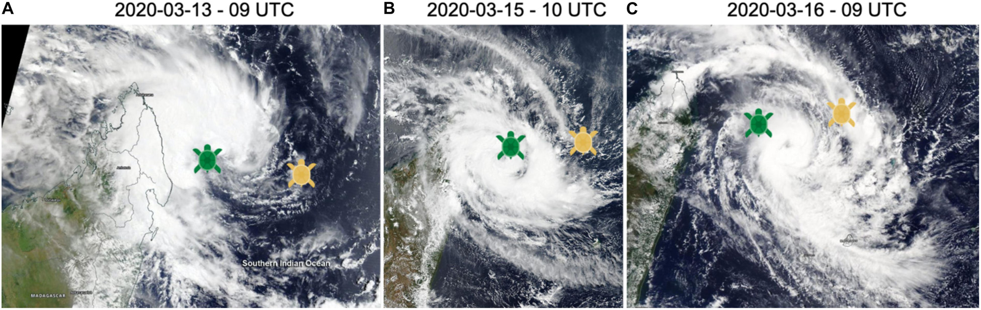
Figure 12. Location of STs “INDIA” (green symbol) and “TOM” (yellow symbol) during the cyclogenesis and intensification phases of tropical cyclone Herold (NE of Madagascar), superimposed on AQUA-TERRA satellite images at (A) 13, (B) 15, and (C) 16 April 2020 at 9, 10, and 9 UTC, respectively.

The third phase of STORM, to be funded by the EU under the INTERREG-V Indian Ocean program, should start in June 2021 and will consist of continuously releasing ∼60–70 ST over a 2-year period at different locations in the basin. This experiment, made possible through the involvement of six regional marine reservations in Seychelles (SE), Mozambique (MZ), Reunion (FR), Comoros (CO), and Terres Australes et Antarctiques Françaises (TAAF), will enable the collection of a unique set of high spatial and temporal resolution temperature and salinity data over most of the SWIO basin. In addition to open ocean areas, which have been the subject of previous STORM observation campaigns, this new phase will make it possible to also collect observations in the Mozambique Channel, a region where in situ observations are quite scarce. The continuous and regular release of STs during a period of 2 years will allow assessing the capability of ST-borne observations to capture the variability of the tropical Indian Ocean (e.g., seasonal and spatial variations of temperature and salinity) as well as to anticipate the onset of large-scale climate anomalies (e.g., Indian Ocean Dipole, Southern Indian Ocean Dipole, SOD) that drive ocean dynamics in this area.

In the present experiment, a high priority was given to the collection of 5-m time series of depth and temperature data. The knowledge and experience gained during the first phase of the program will be used to refine the acquisition procedures as well as to better manage the necessary trade-offs between coverage, temporal resolution and transmitted information, resulting from limited Argos message size and limited battery capacity. In the next phases of STORM, more attention will therefore be devoted to tag programming in order to better exploit their capabilities. For example, a particularly interesting capability of the WC (and other advanced) tags, which was not used in this study, lies in their ability to reconstruct and transmit high-resolution (16-points) mean vertical profiles of depth and temperature over periods of 1 hour, which will be extremely useful for model verification purposes and general ocean studies.

During the forthcoming phases of the STORM project, efforts will also be done to carefully calibrate and intercalibrate hydrographic data obtained from the different tags to be deployed on sea turtles. SMRU tags, whose measurements have been thoroughly analyzed and calibrated when deployed on marine mammals (e.g. Siegelman et al., 2019), will for instance be used as references for intercalibration purposes. This work will be coordinated with AniBOS, the GOOS network on Animal Borne Ocean Sensors (see below). Efforts will also be done to improve profile positioning accuracy, which could be achieved using the newest version of the FoieGras software (Jonsen et al., 2020). Closer interactions with tag manufacturers will also be carried out in order to optimize, and ultimately improve, animal-borne measurements.

Finally, the very recent decision of the Executive Committee of the GOOS Observations Coordination Group (OCG) to create the new sub-network “Animal Borne Ocean Sensors” (AniBOS) opens up new perspectives in terms of biology and oceanographic applications. By offering the possibility to disseminate high quality/frequency observations of physical oceanographic data in a standardized manner, AniBoS will significantly expand the use of biologging data for research and operational applications. In this respect, another important objective of STORM will be to ensure that collected ST datasets will be widely distributed to the ocean science community. Applications envisaged in the medium-term concern, in particular, the assimilation of ST-borne temperature and salinity observations into global and regional ocean models, as well as the provision of consolidated in-situ temperature and salinity observation datasets for satellite and ocean model verification in the tropical IO.

Data Availability Statement

The raw data supporting the conclusions of this article will be made available by the authors, without undue reservation, to any qualified researcher.

Ethics Statement

Ethical review and approval was not required for the animal study because sea turtles were all equipped by qualified personnel (from Kelonia care center and Institute of Ocean and Atmosphere) holding official accreditation to handle and equip these animals. The tags used in STORM meet all the requirements of the international conventions for the protection of sea turtles and were directly purchased from manufacturers specializing in marine biology and biologging. Written informed consent was obtained from the individual(s), and minor(s)’ legal guardian/next of kin, for the publication of any potentially identifiable images or data included in this article.

Author Contributions

OB: writing, project leader, and data analysis. MD and PG: writing and data analysis. MB and SB: data analysis. SC: data collection. ER: writing and data analysis. AV: writing and expertise. All authors contributed to the article and approved the submitted version.

Funding

This study was funded by the European Union, the Regional Council of Reunion Island and the French State under the frame of INTERREG-V Indian Ocean 2014–2020 research project “ReNovRisk-Cyclones and Climate Change,” as well as by CNRS through the LEFE/INSU project “PreSTORM”. This study has been conducted using E.U. Copernicus Marine Service Information.

Conflict of Interest

The authors declare that the research was conducted in the absence of any commercial or financial relationships that could be construed as a potential conflict of interest.

Acknowledgments

We would like to thank the following contributors for their collaboration: Mathieu Barret and the staff of the Kelonia Sea Turtle Care Center; Rui Coelho and the fisheries observers from the Institute for the Ocean and Atmosphere (IPMA, Olhão, Portugal) as well as Jérôme Bourjea (UMR Marbec, IFREMER Sète) for their collaboration in deploying a tag from a Portuguese longline fishing boat, south of Reunion Island; François-Xavier Mayer and the team of the NGO Cétamada (Sainte-Marie, Madagascar) for their priceless help in recovering the tag from the individual poached in Madagascar.

Footnotes

1. ^ Tags deployed on STs TOM and LAZARE ceased emitting in June 2020, but tags deployed on STs TINA and INDIA are still active as of 10 August 2020.
2. ^ Data can be downloaded at https://marine.copernicus.eu.
3. ^ Data can be downloaded at http://www.osi-saf.org.
4. ^ Available from CMEMS at https://resources.marine.copernicus.eu/?option=com_csw&task=results?option=com_csw&view=details&product_id=GLOBAL_ANALYSIS_FORECAST_PHY_001_024.

References

Annamalai, H., Liu, P., and Xie, S.-P. (2005). Variability in SST in the Southwest Indian Ocean: its local effect and remote influence on Asian Monsoons. J. Clim. 18, 4150–4167. doi: 10.1175/JCLI3533.1

CrossRef Full Text | Google Scholar

Bousquet, O., Barbary, D., Bielli, S., Kebir, S., Raynaud, L., Malardel, S., et al. (2020). Evaluation of tropical cyclone forecasts in the southwest Indian Ocean basin using the AROME - Indian Ocean - convective numerical weather prediction system. Atmos. Sci. Lett. 21:e950. doi: 10.1002/asl2.950

CrossRef Full Text | Google Scholar

Brewin, R. J. W., de Mora, L., Billson, O., Jackson, T., Russell, P., Brewin, T. G., et al. (2017). Evaluation of operational AVHRR sea surface temperature data at coastal level using surfers. Estuary Coast. Shelf Sci. 196, 276–289. doi: 10.1016/j.ecss.2017.07.011

CrossRef Full Text | Google Scholar

Cazau, D., Pradalier, C., Bonnel, J., and Guinet, C. (2017). Do Southern elephant seals behave like weather buoys? Oceanography 30, 140–149. doi: 10.5670/oceanog.2017.236

CrossRef Full Text | Google Scholar

Chu, P. C., and Fan, C. (2010). “Objective determination of global ocean surface mixed layer depth,” in Oceans 2010 MTS/IEEE (Seattle, WA), 1001–1007. doi: 10.1109/OCEANS.2010.5663915

CrossRef Full Text | Google Scholar

Ciccione, S., and Bourjea, J. (2010). Discovery of the behaviour of the open sea stages of sea turtles: working the fin by hand with Reunion Island fishermen. Sea Turtle Newslett. 105, 1–6. doi: 10.1515/9780824860196-003

CrossRef Full Text | Google Scholar

Ciccione, S., Jean, C., Carpentier, A., and Barrret, M. (2015). Cause and healing of a sea turtle wound revealed by photo-identification. Indian Ocean Turtle Newslett. 21, 10–12.

Google Scholar

Dalleau, M., Benhamou, S., Sudre, J., Ciccione, S., and Bourjea, J. (2014). The spatial ecology of young loggerhead turtles (Caretta caretta) in the Indian Ocean sheds light on the mystery of “lost years”. Mar. Biol. 161, 1835–1849. doi: 10.1007/s00227-014-2465-z

CrossRef Full Text | Google Scholar

Dare, R. A., and McBride, J. L. (2011). Sea surface temperature response to tropical cyclones. Mon. Wea. Rev. 139, 3798–3808. doi: 10.1175/MWR-D-10-05019.1

CrossRef Full Text | Google Scholar

Davis, R. E., Sherman, J. T., and Dufour, J. (2001). Profiling ALACEs and other advances in autonomous subsurface floats. J. Atmos. Ocean. Technol. 18, 982–993. doi: 10.1175/1520-0426(2001)018<0982:paaoai>2.0.co;2

CrossRef Full Text | Google Scholar

Doi, T., Storto, A., Fukuoka, T., Suganuma, H., and et Sato, K. (2019). Impacts of temperature measurements from sea turtles on seasonal prediction around the Arafura sea. Mar. Sci. 6:719. doi: 10.3389/fmars.2019.00719

CrossRef Full Text | Google Scholar

Dong, S., Sprintall, J., Gille, S. T., and Talley, L. (2008). Southern Ocean mixed- layer depth from Argo float profile. J. Geophys. Res. 113:C06013. doi: 10.1029/2006JC004051

CrossRef Full Text | Google Scholar

Donlon, C. J., Martin, M., Robert-Jones, J., Fiedler, E., and Wimmer, W. (2012). The operational system for sea surface temperature and sea ice analysis (OSTIA). Rem. Sens. 116, 140–158. doi: 10.1016/j.rse.2010.10.017

CrossRef Full Text | Google Scholar

Dujon, A. M., Lindstrom, R. T., and Hays, G. C. (2014). Accuracy of Fastloc-GPS locations and implications for animal tracking. Methods Ecol. Evol. 5, 1162–1169. doi: 10.1111/2041-210x.12286

CrossRef Full Text | Google Scholar

Eyring, V., Bony, S., Meehl, G. A., and Senior, C. (2016). Overview of the design and experimental organization of the Coupled Model Intercomparison Project Phase 6 (CMIP6). Geosci. Model Dev. 9, 1937–1958. doi: 10.5194/gmd-9-1937-2016

CrossRef Full Text | Google Scholar

Gasparin, F., Greiner, E., Lellouche, J.-M., Legalloudec, O., Garric, G., Drillet, Y., et al. (2018). A large-scale view of ocean variability from 2007 to 2015 in the Mercator Ocean global high-resolution monitoring and forecasting system. J. Mar. Syst. 187, 260–276. doi: 10.1016/j.jmarsys.2018.06.015

CrossRef Full Text | Google Scholar

Godley, B. J., Blumenthal, J. M., Broderick, A. C., Coyne, M. S., Godfrey, M. H., Hawkes, L. A., et al. (2008). Satellite tracking of sea turtles: where have we been and where are we going next? Endangered Species Research 4, 3–22.

Google Scholar

Hermes, J. C., and Reason, C. J. C. (2008). Annual cycle of the Southern Indian Ocean Thermocline Ridge (Seychelles-Chagos) in a regional ocean model. J. Geophys. Res. 113:C04035. doi: 10.1029/2007JC004363

CrossRef Full Text | Google Scholar

Hermes, J. C., and Reason, C. J. C. (2009). The sensitivity of the Seychelles-Chagos thermocline ridge to large-scale wind anomalies. ICES J. Mar. Sci. 66, 1455–1466. doi: 10.1093/icesjms/fsp074

CrossRef Full Text | Google Scholar

Hoareau, L., Ainley, L., Jean, C., and Ciccione, S. (2014). Ingestion and defecation of marine debris by loggerhead turtles, Caretta caretta, from bycatch in the southwest Indian Ocean. Mar. Pollut. Bull. 84, 90–96. doi: 10.1016/j.marpolbul.2014.05.031

PubMed Abstract | CrossRef Full Text | Google Scholar

Jeffers, V. F., and Godley, B. J. (2016). Satellite tracking of sea turtles: how do we find our way to the conservation dividend? Biol. Conserv. 199, 172–184. doi: 10.1016/j.biocon.2016.04.032

CrossRef Full Text | Google Scholar

Jonsen, I., Patterson, T. A., Costa, D. P., Doherty, P. D., Godley, B. J., James, W., et al. (2020). A continuous-time state-space model for rapid quality-control of Argos locations from animal-borne tags. Mov. Ecol. 8:31. doi: 10.1186/s40462-020-00217-7

PubMed Abstract | CrossRef Full Text | Google Scholar

Jonsen, I. D., McMahon, C. R., Patterson, T. A., Auger-Méthé, M., Harcourt, R., Hindell, M. A., et al. (2019). Movement responses to the environment: rapid inference of variation among southern elephant seals using a mixed effects model. Ecology 100:e02566.

Google Scholar

Lellouche, J.-M., Greiner, E., Le Galloudec, O., and Garric, G. (2018). Recent updates of the Copernicus marine service’s real-time global ocean monitoring and forecasting system 1/12° at high resolution. Ocean Sci. 14, 1093–1126. doi: 10.5194/os-14-1093-2018

CrossRef Full Text | Google Scholar

Leroux, M.-D., Meister, J., Mekies, D., and Doria, A.-L. (2018). A climatology of tropical systems in the southwest Indian Ocean: their number, trajectories, impacts, sizes, empirical maximum potential intensity and changes in intensity. J. Appl. Meteorol. Clim. 57, 1021–1041. doi: 10.1175/JAMC-D-17-0094.1

CrossRef Full Text | Google Scholar

Lopez, R., Malard, J.-P., Royer, F., and Gaspar, P. (2013). Improving Argos doppler location using multiple-model Kalman filtering. IEEE Trans. Geosci. Remote Sens. 52, 4744–4755. doi: 10.1109/TGRS.2013.2284293

CrossRef Full Text | Google Scholar

Madec, G., Bourdallé-Badie, R., and Chanuta, J. (2019). Nemo Ocean Engine. Notes From the Pôle de Modélisation. France: Institut Pierre-Simon Laplace.

Google Scholar

March, D., Boehme, L., Tintoré, J., Vélez-Belchi, P. J., and Godley, B. J. (2020). Towards the integration of animal-based instruments into global ocean observing systems. Glob. Change Biol. 26, 586–596. doi: 10.1111/gcb.14902

PubMed Abstract | CrossRef Full Text | Google Scholar

Manola, I., Selten, F. M., de Ruijter, W. P. M., and Hazeleger, W. (2015). The ocean-atmosphere response to wind-induced thermocline changes in the tropical South Western Indian Ocean. Clim. Dyn. 45, 989–1007. doi: 10.1007/s00382-014-2338-7

CrossRef Full Text | Google Scholar

Martin, M., Dash, P., Ignatov, A., and Banzon, V. (2012). Group for comparisons of high-resolution sea surface temperature fields of analysis (GHRSST). Part 1: a GHRSST Multi-Product Set (GMPE). Deep-Sea Res. II 77-80, 21–30. doi: 10.1016/j.dsr2.2012.04.013

CrossRef Full Text | Google Scholar

Matyas, C. J. (2015). Formation and movement of tropical cyclones in the Mozambique channel. Int. J. Climatol. 35, 375–390. doi: 10.1002/joc.3985

CrossRef Full Text | Google Scholar

Mavume, A. F., Rydberg, L., and Lutjeharms, J. R. E. (2008). Climatology of tropical cyclones in the southwestern Indian Ocean; landfall in Mozambique and Madagascar. West. Indian Ocean J. Mar. Sci. 8, 15–36. doi: 10.4314/wiojms.v8i1.56672

CrossRef Full Text | Google Scholar

McMahon, C. R., Autret, E., Houghton, J. D. R., Lovell, P., Myers, A. E., and Hays, G. C. (2005). On-board animal sensors successfully capture the real-time thermal properties of ocean basins. Limnol. Oceanogr. Methods 3, 392–398. doi: 10.4319/lom.2005.3.392

CrossRef Full Text | Google Scholar

McPhaden, M. J., Meyers, G., Ando, K., Masumoto, Y., Murty, V. S. N., Ravichandran, M., et al. (2009). RAMA: the research moored array for african-asian-australian monsoon analysis and prediction. Bull. Am. Meteor. Soc. 90, 459–480. doi: 10.1175/2008BAMS2608.1

CrossRef Full Text | Google Scholar

Miyazawa, Y., Kuwano-Yoshida, A., Doi, T., and Nishikawa, H. (2019). Temperature profiling measurements by marine turtles improve estimates of ocean conditions in the Kuroshio-Oyashio confluence region. Ocean Dyn. 69, 267–282. doi: 10.1007/s10236-018-1238-5

CrossRef Full Text | Google Scholar

Mogensen, K. S., Magnusson, L., and Bidlot, J.-R. (2017). Sensitivity of tropical cyclones to ocean coupling in the ECMWF coupled model. J. Geophys. Res. Oceans 122, 4392–4412. doi: 10.1002/2017JC012753

CrossRef Full Text | Google Scholar

Narazaki, T., Sato, K., and Miyazaki, M. (2015). Summer migration to temperate foraging habitats and active winter diving of juvenile loggerhead turtles Caretta caretta in the western North Pacific. Mar. Biol. 162, 1251–1263. doi: 10.1007/s00227-015-2666-0

CrossRef Full Text | Google Scholar

OSI/SAF. (2018a). GHRSST Level 3C of the Indian Ocean Skin Sea Surface Temperature (SST) From the Rotationally Enhanced Visible and Infrared Imager (SEVIRI) on MSG11 in GDS2 Format Produced by OSISAF. Darmstadt: EUMETSAT SAF on Ocean and Sea Ice.

Google Scholar

OSI/SAF (2018b). L3C Hourly Sea Surface Temperature (GHRSST) Data Record Release 1 - MSG. Darmstadt: EUMETSAT SAF on Ocean and Sea Ice.

Google Scholar

Patel, S. H., Barco, S. G., Crowe, L. M., Manning, J. P., Matzen, E., Smolowitz, R. J., et al. (2018). Loggerhead turtles are good observers of the ocean in stratified mid-latitude regions. Estuar. Coast. Shelf Sci. 213, 128–136. doi: 10.1016/j.ecss.2018.08.019

CrossRef Full Text | Google Scholar

R Core Team (2019). A Language and Environment for Statistical Computing. Vienna: R: Foundation for Statistical Informatics.

Google Scholar

Roquet, F., Williams, G., Hindell, M. A., Harcourt, R., McMahon, C., Guinet, C., et al. (2014). A Southern Indian Ocean database of hydrographic profiles obtained with instrumented elephant seals. Nat. Sci. Data 1:140028. doi: 10.1038/sdata.2014.28

PubMed Abstract | CrossRef Full Text | Google Scholar

Roquet, F., Wunsch, C., Forget, G., Heimbach, P., Guinet, C., Reverdin, G., et al. (2013). Animal-enhanced estimates of the Southern Ocean General Circulation. Geoph. Res. Lett. 40, 6176–6180. doi: 10.1002/2013GL058304

CrossRef Full Text | Google Scholar

Siegelman, L., Roquet, F., Mensah, V., Rivière, P., Pauthenet, E., Picard, B., et al. (2019). Correction and accuracy of high- and low-resolution CTD data from animal-borne instruments. J. Atmos. Oceanic Technol. 36, 745–760. doi: 10.1175/JTECH-D-18-0170.1

CrossRef Full Text | Google Scholar

Vialard, J., Foltz, G., McPhaden, M., Duvel, J.-P., and de Boyer Montégut, C. (2008). Strong Indian Ocean sea surface temperature signals associated with the Madden-Julian Oscillation in late 2007 and early 2008. Geophys. Res. Lett. 35:L19608. doi: 10.1029/2008GL035238

CrossRef Full Text | Google Scholar

Vitart, F., Ardilouze, C., Bonet, A., Brookshaw, A., Chen, M., Codorean, C., et al. (2017). The seasonal to sub-seasonal forecast project database. Bull. Am. Meteor. Soc. 98, 163–173. doi: 10.1175/BAMS-D-16-0017.1

CrossRef Full Text | Google Scholar

Xie, S.-P., Annamalai, H., Schott et, F. A., and McCreary, J. P. (2002). Structure and mechanisms of south Indian climate variability. J. Clim. 9, 840–858. doi: 10.1175/1520-0442(1996)009<0840:AOGMPU>2.0.CO;2

CrossRef Full Text | Google Scholar

Yang, G.-Y., and Slingo, J. (2001). The diurnal cycle in the tropics. Mon. Wea. Rev. 129, 784–801. doi: 10.1175/1520-04932001129<0784:TDCITT<2.0.CO;2

CrossRef Full Text | Google Scholar

Yokoi, T., Tozuka, T., and Yamagata, T. (2008). Seasonal variation in the seychelles dome. J. Clim. 21, 3740. doi: 10.1175/2008JCLI1957.1

CrossRef Full Text | Google Scholar

Zhang, H.-M., Reynolds, R. W., Lumpkin, R., Molinari, R., Arzayus, K., Johnson, M., et al. (2009). An integrated global ocean observing system for sea surface temperature using satellites and in situ data: from research to exploitation. Bull. Am. Meteorol. Soc. 90, 31–38. doi: 10.1175/2008BAMS2577.1

CrossRef Full Text | Google Scholar

Zhang, H.-M., Reynolds, R. W., and Smith, T. M. (2006). Adequacy of the in situ observing system in the satellite age for climate ESS. J. Atmos. Ocean. Technol. 23, 107–120. doi: 10.1175/JTECH1828.1

CrossRef Full Text | Google Scholar

Appendix

Diving Behavior of STs Brice and Samson

In addition to the time series of depth/temperature data used in this study, additional products such as histograms of “time at depth,” “time at temperature,” “minimum and maximum dive depth,” and “dive duration” over user-defined bins and time periods can also be obtained from WC tags to investigate the diving behavior of instrumented animals. Information derived from such histogram data is presented hereafter to provide general information on the diving behavior of STs SAMSON and BRICE over approximately 7 months (February 15–August 30 2019 vs. April 2–October 31 2019, respectively). The two animals shared approximately the same morphometric characteristics (see Table 1) and crossed the Indian Ocean a few months apart while following the same trajectory until they crossed the equator (Figure 2).

Nine hundred eighty-four (resp. 892) histograms containing diving data aggregated over periods of 3 h have been transmitted by ST BRICE (resp. SAMSON), which represents an accumulated time period of ∼123 (resp. 112) days. This number of files correspond to ∼58% (resp. 56%) of the theoretical number that would be expected assuming an Argos transmission efficiency of 100%. The summary of diving data is given in Table A1. Note that because the tags used in this study were setup to only record dives deeper than 10m, the number of recorded dives is incomplete and is thus not representative of the true diving behavior of the animals.

TABLE A1

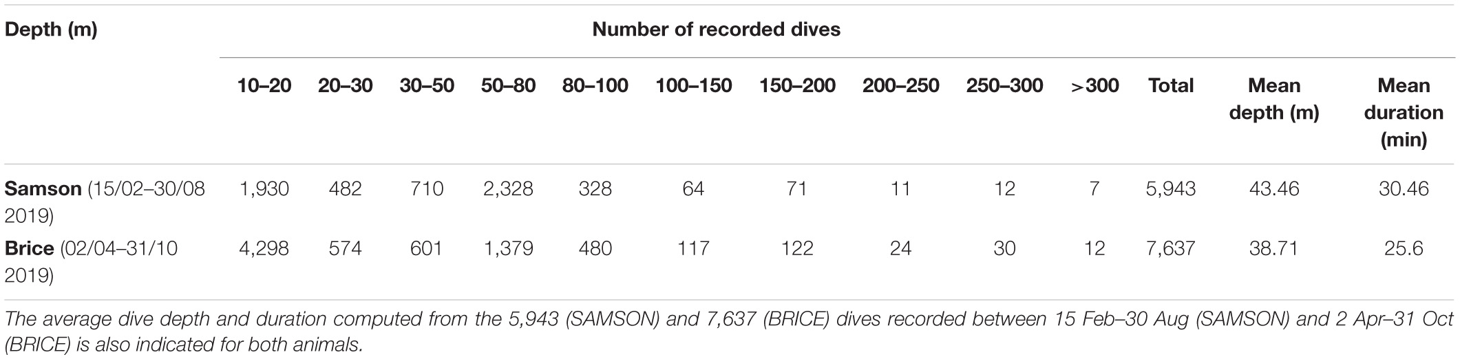
Table A1. Diving behavior of sea turtles SAMSON and BRICE. Number of recorded dives >10 m classified by depth layers.

Recorded data (Table A1) show that ST BRICE (resp. SAMSON) made 7,637 (resp. 5,943) dives >10 m over its 7-month (resp. 6.5-month) sampling period. These figures indicate that ST BRICE made about 30% more dives below 10m than ST SAMSON (62 vs. 53 dives/day on average). SAMSON’s dives, however, lasted longer (30 vs. 24 min) and were also 15% deeper (43 vs. 38 m) on average. Data also indicate that ST BRICE made significantly more deep dives (>100 m) than ST SAMSON. This behavior appears more clearly in Figure A1, which shows time series of maximum depth data recorded during the sampling period of both animals. According to these records, the diving behavior of these two STs thus appears rather different. While diving behavior is generally animal-dependent, the distinct environmental conditions encountered by the two animals during their journey toward the Gulf of Oman have also likely impacted on both animal diving habits.

FIGURE A1

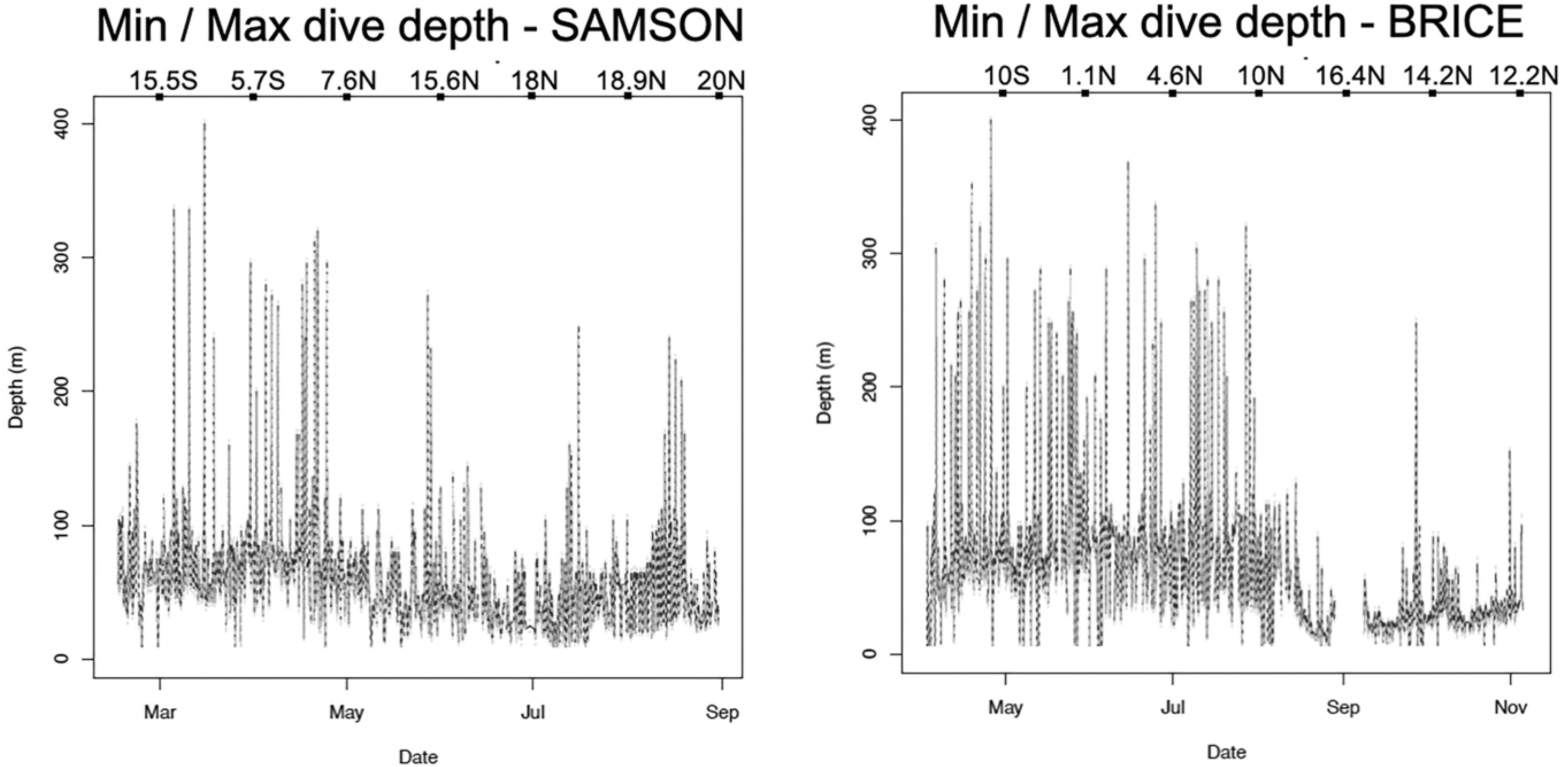
Figure A1. Time series of daily maximum dive depths (>10 m) for STs SAMSON (left panel, 15 Feb–30 Aug) and BRICE (right panel, 2 Apr–31 Oct). The position in latitude of the two animals at the beginning of each month is indicated on the top of each panel.