Very High Resolution Tools for the Monitoring and Assessment of Environmental Hazards in Coastal Areas

1. Introduction

On Friday 21st April 2017, the passenger ferry “Volcán de Tamasite” collided with the “Nelson Mandela” dike of the Port of La Luz (Las Palmas de Gran Canaria) at 7:00 p.m. As a consequence of the impact, two of the outermost fuel supply pipes along the dike were broken and diesel fuel poured into the sea. The national pollution alert was declared at 7:30 p.m., and the company responsible for the pipelines started working on emptying the damaged pipes. These works ended on the 24th of April 2017. Around 65 m³ of diesel fuel was estimated to be spilled along the Northeastern (NE) sector of Gran Canaria island. The rate of evaporation/dispersion ranged from 80% by day. On the 23rd of April at 7:00 a.m., satellite images reported the two major spill spots targeted near the coast. Both spots, of 0.9 and 2.4 km², respectively, were dispersed at ground level at the NE sector of the island, 12 km far south from the Port of La Luz, by the Maritime Security Service fleet (SASEMAR). Consistently, on this day, local newspapers reported a 13 km long fuel filament placed 1 km far away, at the east of Gran Canaria (TeldeActualidad/EFE, 2017). The national pollution alert ended on the 25th of April, although the monitoring and surveillance along the eastern sector of the island continued until the 5th of May. Along these days, some scarce and dispersed pollutant spots were reported and tracked by aerial and marine surveys some miles away from the coast until that date, when the event was officially declared as “finished” (CIAIM, 2018). Figure 1 displays the ferry crash point (in red) together with some specific coastal areas, where the arrival of pollution could have a very negative impact (in magenta, green and blue). These vulnerable areas are: Las Canteras, a beach in the city of Las Palmas, along with a desalinization plant, a fish farm, and a thermoelectric plant, all in the eastern coast of the island.

FIGURE 1

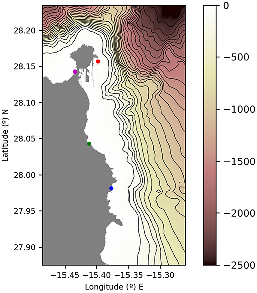
Figure 1. A map of the N-NE Gran Canaria Coast, displaying the ferry crash point (red) together with some highly vulnerable regions. These areas are: Las Canteras beach in the city of Las Palmas (magenta), a desalinization/hydroelectric power plant (green), and the Port of Taliarte (fishing and aquaculture facilities) (blue). Contourlines represent the bathymetry in meters.

Pollutant transport monitoring in coastal areas is essential because of the many critical activities occurring in them. Recently, it has been reported how the analysis of ocean currents, which are operationally delivered by ocean forecasting services (De Dominicis et al., 2016), combined with the use of remote sensing techniques (Cheng et al., 2011; Marta-Almeida et al., 2013; Xu et al., 2013) and dynamical systems tools (Olascoaga and Haller, 2012; García-Garrido et al., 2016) are capable of providing important feedback to emergency services. Currently, synergies between these capabilities for coastal applications are flourishing due to the fact that remote sensing and modeling capabilities are reaching very resolved metric scales, thus providing the bedrock for future smart coasts.

Remote sensing capabilities allow for a direct observation of extended areas. The limitations of these capabilities are due to the satellite swath, revisit time, atmospheric conditions and cloud coverage for optical sensors. During the reported event, optical images from Sentinel 2 and Landsat 7 and 8 were available and analyzed. These specific image products were useful in the past for oil spill monitoring (Pisano et al., 2015; García-Garrido et al., 2016) and we explore their potential in this study. Additionally, Synthetic Aperture Radar (SAR) images have been demonstrated to be a very adequate tool for remote detection of oil spills (Cheng et al., 2011; Xu et al., 2013; Pisano et al., 2015), specially due to their high spatial resolution and all-weather and all-day capabilities. During this case study, SAR images from Sentinel 1A and 1B were available. Spatial resolution of Sentinel 1 and 2 is very high (up to 10 m), while that of Landsat 7 and 8 is lower (up to 30 m).

Ocean model products also provide direct information on extensive areas. To perform this study, we have used two modeled data sources for ocean currents in the area of interest: (1) The regional forecast product for the IBI (Iberia-Biscay-Ireland) area, operationally delivered by the CMEMS Service and (2) a very high resolution coastal model system, specifically developed by Puertos del Estado (PdE) for the Port of La Luz. The IBI product shows a kilometric resolution (derived from the 1/36° NEMO model application), too coarse for the coastal event under study. Nevertheless, we have applied the PdE ROMS model application that downscales the regional IBI solution for the Gran Canaria area by means of 2 nested grids (a coastal one, with ~ 350 m horizontal resolution, which we refer to as the CST model, and a very high resolution local domain, specifically focused on the Puerto de la Luz area with ~ 40 m resolution, which we refer to as the PRT model). Transport processes associated with these currents are subject to uncertainties, such as those inherent in the modeled velocity fields, as they depend on assumptions taken in the modeling processes. Each result on the velocity fields produced by different model hypotheses may characterize pollutant dispersion differently, and thus we address the issue on how to compare outputs. Our analysis goes beyond the tracking of individual pollutant trajectories by exploiting ideas from dynamical systems theory that involve the determination of geometrical structures in the ocean surface which define regions where fluid particle trajectories have qualitatively distinct dynamical behavior (Wiggins, 2005; Mancho et al., 2006; García-Garrido et al., 2015, 2016; Balibrea-Iniesta et al., 2019). These geometrical structures provide a signature for a specific velocity field, highlighting the essential transport features associated to it.

This paper is organized as follows. Section 2 describes the data sources used in this work: satellite data, ocean models and the transport problem. Section 3 presents the results, a discussion on how the dynamical systems approach supports the interpretation of transport, and a discussion on uncertainty quantification. Finally, Section 4 reports the conclusions of this work.

2. Data and Methodology

2.1. Satellite Imagery and Remote Sensing

The following high-resolution satellite image data sources, corresponding to the dates for which the “Volcán de Tamasite” ferry crash event took place, were downloaded (at no cost) and adequately processed:

• SAR data from Sentinel 1 (A,B), Level-1 IW GRDH (Interferometric Wide Swath Ground Range Detected) with high resolution, was obtained from the Sentinel Data Hub (https://scihub.copernicus.eu/).

• Sentinel 2A MultiSpectral Instrument (MSI) Level 1C data was also downloaded from the Sentinel Data Hub.

• Landsat 7 ETM+ (Enhanced Thematic Mapper Plus) and Landsat 8 OLI (Operational Land Imager) level 1C data was downloaded from the U.S. Geological Survey (https://earthexplorer.usgs.gov/).

The images were processed using the following tools. Sentinel 1 data was processed using SNAP (https://step.esa.int/main/toolboxes/snap/) SAR tools. Sentinel 2 MSI, Landsat 7 ETM+ and Landsat 8 OLI were processed using the Acolite toolbox (Vanhellemont, 2019). The chronological sequence of satellite images available during the event is provided in the following list:

• 04/21/2017: Sentinel 1B, 7:04 p.m., a few minutes prior to the accident.

• 04/23/2017: Sentinel S1A 07:00 a.m., in situ confirmed spill patterns were weakly visible.

• 04/26/2017: Landsat 8 11:30 a.m., cloudless, no spill patterns identified.

• 04/27/2017: Sentinel 1A 7:00 p.m., no spill patterns identified.

• 04/29/2017: Sentinel 1B 07:00 a.m., no spill patterns identified.

• 05/01/2017: Sentinel 2A 11:50 a.m., cloudy.

• 05/03/2017: Sentinel 1B 7:00 p.m., no spill patterns identified.

• 05/04/2017: Landsat 7 11:30 a.m., no spill patterns identified.

With the purpose of identifying water discoloration due to the spill, the inspection of optical images was performed both through RGB composites and remote sensing reflectance spectra. However, this analysis did not provide insights for the event, and we do not report further about them. SAR images were also examined. Due to the spreading tasks done by the emergency services and the characteristics of the targeted oil spill, an intense signal was not expected. However, weak patterns (lately confirmed through in-situ observations) were identified on one Sentinel 1A image obtained on Sunday 23rd of April 2017 at 07:00 a.m. At that time, the Spanish coastguard fleet (SASEMAR) had already begun the daily operations (06:00 a.m.). Figure 2 displays this SAR Sentinel-1A image. Figures 2A–C show “low-roughness” spots around NE Gran Canarian waters, indicating potential positions for the diesel oil spill drift, after the ferry crash. The two “low-roughness” spots appearing in the image (marked with red circles in Figures 2A–C) were on ground confirmed spills (and dispersed) by three SASEMAR ships and one helicopter. Indeed, at the time of the Sentinel 1A passing over, two ships confirmed the spill spot at the North, in the vicinity of the Port. The spill spot located 12 km south from the Port, in the neighborhood of the Marine Eolic Platform facility (www.plocan.eu) and 1 km far away from land, drifting southwards, was confirmed by a third ship and one helicopter (CIAIM, 2018).

FIGURE 2

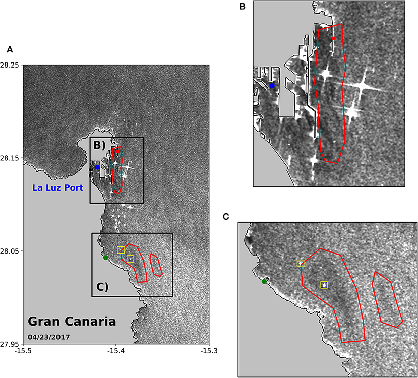
Figure 2. (A) SAR Sentinel-1A image obtained on Sunday 23rd of April 2017 at 07:00 a.m. The image shows two areas with “low-roughness” spots that were ground confirmed spills by three ships and one helicopter of the Spanish Coastguard fleet (SASEMAR), who started to work on the affected areas on that day at 06:00 a.m.; (B) The Northern spilling area (red area) was dispersed in the neighborhood of the Port by two ships. The broken fuel lines were finally closed at 20:30 p.m., several hours after the Sentinel-1B passing over that region (07:00 a.m.); (C) The Southern spilled area reported by the SAR Sentinel-1B was located 12 km south from the Port, in the Marine Eolic Facility (www.plocan.eu) waters. This spill was validated by SASEMAR and coastguard helicopter flights (also reported in the SAR image). Both spots drifted southwards 1 km away from the coast, until the pollution alert ended on the 25th of April at 8:30 a.m. SASEMAR's Airplane, however, continued surveying the whole Eastern coastline of the island until the 8th of May 2017 (CIAIM, 2018).

2.2. Ocean Models

Ocean currents in the area of interest are supplied by two sources. One is the Copernicus Marine Service model for the Iberian-Biscay-Irish region (CMEMS IBI-PHY, IBI hereafter) available from http://marine.copernicus.eu/. Currents obtained from this product in the area of the accident are displayed in Figure 5A), where the accident location is marked with a red dot. IBI outputs have too coarse resolutions for the scale of the event we want to describe. For this reason, we used specific high-resolution modeled currents for the Port of La Luz, downscaling the IBI regional solution through two offline nested domains, with resolutions of 350 m in the intermediate coastal domain (the CST model) and 40 m in the local domain that covers the port waters (the PRT model). Details about the model product configurations and their quality are given next:

• CMEMS IBI-PHY: The CMEMS IBI provides operational regional short-term (5-days) hydrodynamic forecasts of a range of physical parameters (currents, temperature, salinity, and sea level) since 2011 (Sotillo et al., 2015). IBI is based on an eddy-resolving NEMO model application (v3.6) that includes high-frequency processes required to characterize regional-scale marine processes. The model application runs at a 1/36°~2.5km horizontal resolution and final products are routinely delivered in a service domain extending between 26°N and 56°N and 19°W and 5°E, see Figure 3. The NEMO model (Madec and NEMO Team, 2019) solves the three-dimensional finite-difference primitive equations in spherical coordinates discretized on an Arakawa C-grid and 50 geopotential vertical levels (z coordinate), assuming hydrostatic equilibrium and the Boussinesq approximation. Partial bottom cell representation of the bathymetry (a composite of ETOPO2 and GEBCO8) allows an accurate representation of the steep slopes characteristic of the IBI area. The IBI system is forced with up-to-date high-frequency 1/8°~12.5km hourly meteorological forecasts provided by the ECMWF (European Centre for Medium-Range Weather Forecasts). Variables, such as 10 m wind, surface pressure, 2 m temperature, relative humidity, precipitation, shortwave and longwave radiative fluxes are used as forcing, being a CORE empirical bulk formulae (Large and Yeager, 2004) used to compute surface (latent and sensible) heat and freshwater (evaporation-precipitation) fluxes and surface stress.

FIGURE 3

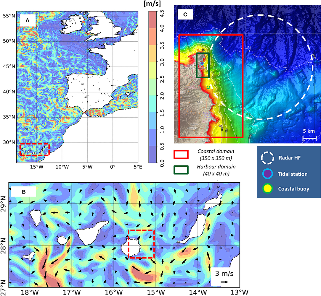
Figure 3. (A) Spatial domain of the IBI-PHY model. The colored areas denote the daily-averaged surface current speed on the 21st April 2017 in units of m/s. The dotted red rectangle encloses the Canary Islands (Spain). (B) Zoom of the Canary Islands for the same surface currents fields depicted in (A). The superposed black arrows represent the surface current field. (C) Nesting strategy for the Port of La Luz. The coastal domain area is enclosed in the red lined rectangle, whereas the local domain is enclosed in the green one. The colored areas show the bathymetry. The white dotted circle encloses the PLOCAN surface-current HF radar. The blue dot marks the tidal station within the harbor; whereas the yellow one marks the coastal buoy (Puertos del Estado monitoring network).

The IBI regional system is nested into the CMEMS Global solution, using as open boundary conditions daily outputs from this CMEMS global eddy resolving system. Tidal solution is also added at the boundaries (at that time, IBI system was using 11 tidal harmonics). An atmospheric pressure component is also included assuming pure isostatic response at open boundaries (inverse barometer approximation). The CMEMS IBI system uses a SAM2-based data assimilation scheme to enhance its predictive skills by constraining the model in a multivariate way with a wealth of observations: Altimeter data (i.e., along-track sea level anomalies), in-situ temperature and salinity vertical profiles and satellite-derived sea surface temperature are regularly assimilated to estimate periodically initial conditions. Further details on the data assimilation scheme and on the analysis generated can be seen in the CMEMS IBI Product User Manual report (Amo et al., 2020), available at CMEMS, where more details of the operational suite can be found.

We have used the data set IBI_ANALYSIS_FORECAST_PHYS_005_001 with horizontal resolution of 1/36°~2.5km on a regular latitude/longitude equirectangular projection of the Northwest African waters domain. Daily 3D fields are available over 50 geopotential vertical levels, but in this study hourly fields provided for the upper layer are used (Aznar et al., 2016). The IBI ocean model forecasts are continuously monitored, using to this aim the NARVAL multi-parameter multi-platform validation toolbox (Lorente et al., 2019). This multi-parametric ocean model skill assessment is performed by the IBI-MFC using all available operational observational sources in the IBI model domain. The list of observational data source used in the IBI validation includes remote sensed data (i.e., satellite L3 and L4 SST and sea level anomaly products, together with surface currents from coastal HF-Radars stations) and in-situ observations (from moorings and tide gauges and sea level essential variables such as surface temperature, salinity, currents and sea level; as well as from ARGO floats for 3D temperature and salinity). See further details in Lorente et al. (2019) for a complete list of the observational products and platforms used, as well as the regions covered, to operationally validate the IBI ocean model product. Furthermore, the CMEMS IBI-MFC forecast model products are qualified before their entry into operational service. Main results from this scientific qualification of the IBI ocean model products can be seen in the comprehensive product quality document delivered together with the IBI product (the CMEMS IBI-MFC Quality Information Document, available online Sotillo et al., 2020a). This product quality report points out the good agreement on average between the model system and the available observations. Being particularly true for sea level when compared to along-track altimetry and tide gauge stations (in these coastal stations, model tidal and residual sea level measures are also close to the tide gauge observations used). The comparison with in-situ temperature-salinity profiles, all of them off-the-shelf, also shows good IBI model performances, especially below the thermocline. In the Canary Island region, model differences with observations are low (root mean square errors (RMSE) and biases of 0.45 °C and 0.07 °C and 0.15 and 0.01 psu, for temperature and salinity, respectively; values obtained from the comparison of IBI with full ARGO profiles during the 2-year period 2013–2015). Concerning the Sea Surface Temperature (SST), the IBI system performs well in average, but can locally display high biases. Thus, RMSE computed over the whole IBI domain over a 6-year period is around 0.6 °C. This IBI referential product quality report shows also some IBI metrics for surface currents. However, it warns about the difficulty to assess such variable, mostly due to the very scarce availability of long time series of velocity measurements, and the very limited representativity of such measurements (there are only a few local measurements available, making it impossible to build regional metrics for surface currents, such as the ones provided for the SST and sea level fields or the 3D temperature and salinity).

• PdE La Luz Port model: CMEMS IBI provides a regional solution at kilometric scales. The IBI horizontal resolution in clearly not enough to characterize coastal events such as the one we discuss in this work. Therefore, a local high-resolution dataset is needed to characterize circulation patterns in the Puerto de la Luz. In the framework of the H2020 IMPRESSIVE Project, PdE has developed a new model setup for this port, covering also nearby waters along the Eastern coast of Gran Canaria island. This newly developed model setup, with a very high resolution, has been specifically designed for the Puerto de la Luz, and used by PdE to test some model updates that will be used in the future to upgrade the PdE SAMOA port forecast systems (Sotillo et al., 2020b), currently implemented and running operationally in different Spanish Port Authorities. The high-resolution hydrodynamic module is based on the ROMS (Shchepetkin and McWilliams, 2005) model (version 3.7). ROMS is a time split-explicit, free-surface, terrain-following-coordinate oceanic model that has been applied successfully for oceanographic forecasting at other Spanish harbors (Grifoll et al., 2012). The proposed nesting strategy comprises two off-line nested domains: a coastal one nested with IBI with a horizontal resolution of 350 m and ranging from shallow waters to water depths around 2000 m (hereafter coastal model); and a local one (with a horizontal resolution of 40 m), nested in the previous one (hereafter local model). We illustrate it in Figure 3. Due to the sudden sharp slope gradients at the continental shelf, the vertical discretization has been setup at 30 sigma levels for the coastal model. At the local model, 15 sigma levels were found to be enough for handling the bathymetry. The vertical discretization follows the S-coordinate system described in Song and Haidvogel (1994). The bathymetry for both domains was built using a combination of bathymetric data from EMODNET (with an approximate resolution of 230 m) and from specific local high-resolution sources provided by the local Port Authority. Furthermore, within a transition region (2 km) along the open boundaries of the coastal model, the bathymetry from the CMEMS-IBI system is used to accommodate the high-resolution information and keep consistent the transports associated with IBI velocities imposed as open boundary conditions. In the local model, an updated and higher resolution bathymetry is also applied, adjusting the open boundary to the coastal bathymetries. The bathymetry information interpolated over the mesh is smoothed using a Shapiro filter (Shapiro, 1970) with an r-factor criterion below 0.25. The bottom boundary layer has been parameterized with a logarithmic profile using a characteristic bottom roughness height of 0.002 m. The turbulence closure scheme for the vertical mixing is the generic length scale (GLS) tuned to behave as k-ε (Warner et al., 2005). Horizontal harmonic mixing of momentum is defined with constant values of 5m²/s. Moreover, the atmospheric forcings come from the HARMONIE model (Bengtsson et al., 2017) with spatial resolution of 2.5 km. The following atmospheric variables are used: wind fields, sea-level pressure, temperature at 2 m elevation, relative humidity at 2 m elevation, precipitation, long wave and solar radiation.

With respect to the quality assessment of very high resolution coastal model systems, covering a very limited spatial domain such as the one we present here for La Luz Port, it is important to remark that one of the main bottlenecks identified is the lack of an adequate near-real-time delivery of operational observations. This lack of operational observations, specially on coastal areas, restricts the systematic production and exploitation of quality assessments of operational ocean model products such as the ones used here. Indeed, in a recent review performed by EuroGOOS for European coastal operational ocean model services (Capet et al., 2020), it is pointed out that only 20% of operational models currently available for European seas provide a dynamic uncertainty together with their forecast products. Unfortunately, this is the case in terms of validation of the Port of La Luz model currents for the dates (21-23 April 2017) of the event here studied. There is no option to analyze the quality of the surface current modeled fields for such specific dates due to the lack of in-situ or remote sensing observations in the area. Nevertheless, there is some information on the model dynamical performance derived from other validation exercise performed on different essential ocean variables and temporal periods that can illustrate the capability of the model setup proposed to reproduce the coastal dynamics in the area.

As previously mentioned, the Coastal and Port model systems implemented in La Luz Port are an evolution of the PdE operational SAMOA model setup, used for operational forecasting in the island of Gran Canaria (Sotillo et al., 2020b). In this work, the quality of 1-year SAMOA ocean forecast products (operationally available for 9 Spanish Ports) was assessed by comparison with observations, both from in-situ moorings and remotely sensed products. It is important to highlight how the SAMOA model systems focused on the Canary Islands (4 out of 9 SAMOA system existing at that time) show the best agreement for SSH when compared to hourly sea level observations from tide gauges (with reported correlation coefficients around 0.98 and RMSE that ranges between 0.07 and 0.16 m). The performance of coastal SAMOA systems appears to be rather consistent in terms of SST, according to the skill metrics obtained (correlation values above 0.89 and RMSE usually in the range 0.2−−0.4 °C, considering more than 3,200 hourly observations for each case). Indeed, the SAMOA system running in Gran Canaria shows the second best performance of a PdE SAMOA operational model when compared to hourly SST observations from a coastal buoy (in this case, moored close to the Port of La Luz).

Currently, PdE is working on a similar model setup as the one we have used for the analysis of the Tamasite event, validating their model system with several observational data sources available over that period (i.e., HF Radar and in-situ mooring).

2.3. The Transport Problem

The transport process of oil particles can be described by a concentration field C(x, t) which depends on time t and the position x. The position x, has three components considering that oil particles move on the ocean surface and may also sink. The evolution of the concentration C(x, t) is affected by the flow, represented by the velocity field v(x, t), and molecular diffusion. It is described by the following advection-diffusion equation (De Dominicis et al., 2013):

$\begin{array}{ll}\frac{\partial C}{\partial t}+\text{v}·\nabla C=D{\nabla }^{2}C,& (1)\end{array}$

Here D is the is the molecular diffusion coefficient. At the ocean scale, the diffusion transport is much smaller than the convective transport (Monroy, 2019) and hence the Equation (1) reduces to:

$\begin{array}{ll}\frac{dC}{dt}=0,& (2)\end{array}$

where d/dt is the total time derivative. Equation (2) implies that the quantity C is conserved along fluid parcel trajectories and behaves as a passive tracer. Particles with a finite size and different density to that of water may not instantly follow fluid velocities. Other mechanisms besides passive advection contribute to their transport, such as gravity forces, their finite size, inertia and history dependence (Maxey and Riley, 1983; Cartwright et al., 2010). Results in Monroy et al. (2017) confirm, however, that for a wide range of particles that sediment in turbulent ocean flows, the description of passive tracers is appropriate, except for the addition of a constant vertical velocity arising from the particle weight. In particular, for the case of the diesel fuel under study, weight effects are negligible and therefore we considered that it follows fluid parcels. This approach is rather reasonable for diesel fuel since it is less dense than salty water and moves mainly horizontally, close to the surface, slightly below the waterline, and thus it is not subjected to direct wind sailing effects. Studies such as (Lekien et al., 2005; Olascoaga and Haller, 2012; García-Garrido et al., 2016) confirm that considering advection as the dominant contribution to pollutant transport provides very good results.

Fluid parcels follow trajectories x(t) on the ocean surface that evolve according to the dynamical system:

$\begin{array}{ll}\frac{d\text{x}}{dt}=\text{v}(\text{x},t),& (3)\end{array}$

where the position is described in longitude (λ) and latitude (ϕ) coordinates, that is, x = (λ, ϕ), and v represents the velocity field. In longitude/latitude coordinates, the dynamical system in Equation (3) can be rewritten as:

$\begin{array}{ll}\{\begin{array}{c}\frac{d\lambda }{dt}=\frac{u(\lambda ,\varphi ,t)}{Rcos\varphi }\\ \frac{d\varphi }{dt}=\frac{v(\lambda ,\varphi ,t)}{R}\end{array},& (4)\end{array}$

where R is the Earth's radius. This equation assumes that the vertical velocity component in the ocean is small compared to the horizontal ones and for that reason it has been disregarded. The two velocity components are determined by the zonal (u) and meridional (v) velocities, which are obtained from the different ocean models: IBI, CST, and PRT. We have tracked fluid parcels that evolve according to velocities supplied by these three models. Due to the limitations of CST or PRT models in terms of spatial domain (the PRT domain is only focused on inner port waters and the nearby ones, and CST is focused on an area of the coast, see Figure 3) in order to be able to track fluid parcels outside their geographical coverage, the zonal and meridional velocity fields need to be composed with IBI fields. Figure 4A illustrates a sketch of two grids corresponding to the IBI and CST models. Figure 4B shows the structured grid resulting from the composition of grids in Figure 4A. The grid is made up of cells with areas of different sizes. A linear interpolation is used within each cell to approximate the velocities within them. When the PRT model is used, its grid is nested within the CST grid, which in turn is nested with the IBI grid, i.e, a hierarchy of three nested data is required. The accuracy of this approach is supported, and justified, in the next section, by the agreement between the predictions made by the simulations, the oil sightings from satellite and in-situ observations.

FIGURE 4

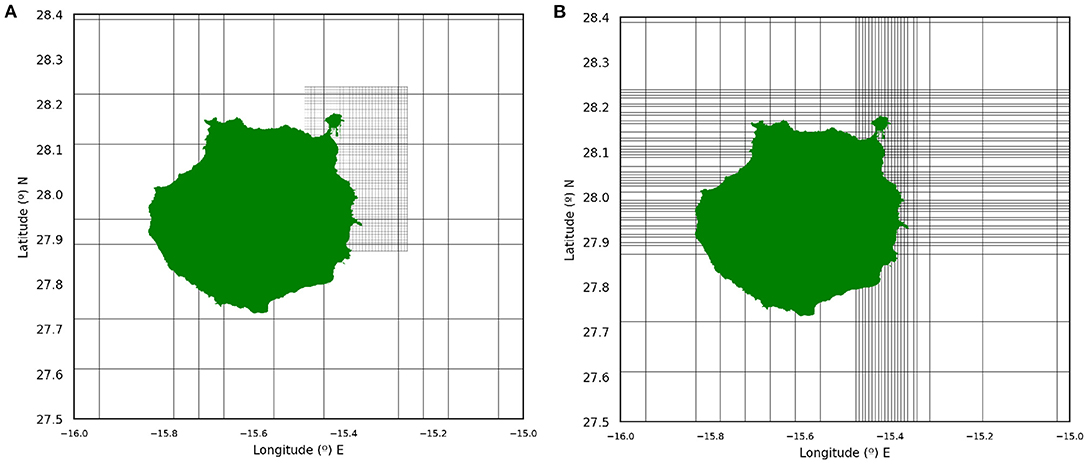
Figure 4. (A) A sketch illustrating the two grids (IBI and CST) represented in the domains where the hydrodynamic models are solved; (B) the composition of the two grids, which results in a structured, non-uniform grid. Within each cell velocities are linearly interpolated.

There exist diverse software packages that are able to track oil spills. Among others, oil drift models include (Cheng et al., 2011; Xu et al., 2013) EUROSPILL, OILMAP (Oil Spill Model and Response System), GNOME (General NOAA Operational Modeling Environment), MOTHY (French operational oil spill drift forecast system), OSCAR (Oil Spill Contingency and Response), ADIOS2 (Automated Data Inquiry for Oil Spills), OSIS (Oil Spill Identification System), and Medslik-II (De Dominicis et al., 2013). These models are focused on tracking individual fluid parcels, and they need to play with a sufficiently large number of initial parcels to maintain a good representation of the spill. Contrary to these oil spill approaches, in this work we track in time the whole area where the fuel is extended, and the algorithm self regulates the number of fluid parcels on the contour to ensure its accurate representation at all times. The area is tracked with contour advection algorithms developed in Dritschel (1989), including some modifications explained in Mancho et al. (2003), Mancho et al. (2004), and Mancho et al. (2006). More specifically, the spill is modeled by an initial contour surrounding an area, A₀, with a given thickness h₀. The product V = A₀·h₀ is the volume of the initial spill. While the contour is advected, the initial area, whose value is typically preserved for 2D incompressible flows, is distorted.

Transformation processes like evaporation, photo oxidation, etc., act on the slick while it drifts. Evaporation is an important process for most oil spills. Oils and fuels are slowly evaporating mixtures of compounds whose long-term behavior are not always well-described by air-boundary layer interaction mechanisms, but through diffusion mechanisms (Fingas, 2014). However, the diesel under consideration has volatile components, that do evaporate via air boundary-layer-regulated mechanisms. Software packages quoted above include models to represent the weathering of the spills according to different oil properties. In our model, oil is presumed to consist of one component and its volume is assumed to decrease through evaporation by diminishing its thickness h₀. In this way spill contours are evolved uncoupled from degrading effects which are considered at representative levels as a change in the intensity color of the oil spill. The intensity will be adjusted depending on the degradation of the specific type of oil. According to McIlroy et al. (2018) and Butler (1976), the fraction of the original diesel compound remaining after evaporation can be adjusted to a kinematic law:

$\begin{array}{ll}\frac{V}{V_0}=e^{-Bt},& (5)\end{array}$

where V₀ is the original volume, and V is the volume at time t. According to in-situ reports, the spill reduced an 80% in approximately 72 h (Montero, 2017), which give us an estimation of the evaporation rate B = 0.02235 h⁻¹.

3. Results and Discussion

The passenger ferry crashed at the position marked by a red dot in Figure 1, located at 28°9.418′ N and 15°23.871′ W. Figure 5 shows a time frame that is representative of the surface current patterns during the event. Throughout the episode, surface currents were mainly driven by large-scale circulation patterns and tides. Current fields were southward, with a modeled daily-averaged current speed of 12-16 cm/s at the eastern shelf of Gran Canaria island. IBI-PHY and the high resolution model presented similar current magnitudes. Note that only the semi-diurnal tidal current range was around 10 cm/s. Currents induced by residual tides can be considered as negligible: from the 21st to the 23rd of April, a negative surge was measured with an average value of 2 cm. At the end of the 23rd of April, though, the negative surge rose to 6 cm. Wind-induced currents had also a secondary role: measured surface wind at the tidal station was mainly from the N-NW sector, with a wind speed of 3.38 m/s (standard deviation of 0.88 m/s). There was no evidence of gustiness, either: average maximum wind speed was mild, with low variability (5.25 m/s with a std. deviation of 1.2 m/s). Finally, wave-induced currents may have had a secondary role: measured waves at the coastal buoy were moderate, with significant wave height of around 1.1 m and maximum wave heights of 1.5 m. The peak period was close to 8 s, exhibiting a young swell sea-state.

FIGURE 5

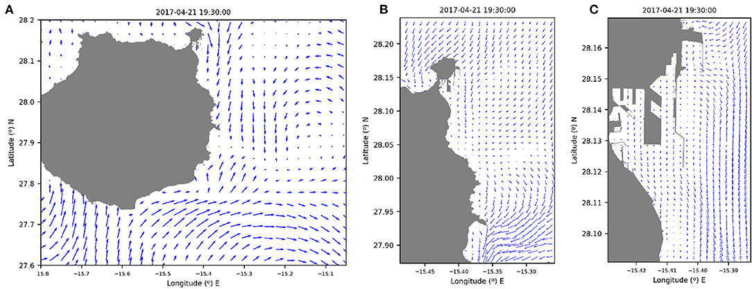
Figure 5. Currents in the Gran Canaria coast at different resolutions. (A) Currents by the IBI model; (B) currents in the high resolution CST model; (C) currents in the very high resolution PRT model.

On the 23rd of April 2017 at 7:00 a.m., remote sensing images confirmed the spreading of the diesel fuel southwards, (see Figure 2). This is consistent with the evolution of the spill, which is modeled as a blob at the accident location, according to the three models: IBI, CST, and PRT. Figure 6 illustrates this point. Figure 6A shows how it evolves according to IBI model, Figure 6B illustrates the evolution according to the CST model nested in IBI data, and finally (Figure 6C) displays the evolution according to the PRT model nested in CST and in IBI data. Arrows mark the position of the blob at successive times. The color degradation from black to white, in a gray scale represents the evaporation. All three models predict a southwards evolution, although IBI model drifts southwards faster than the others and at the observation time, i.e., 23rd of April 2017 at 7:00 a.m., the spill is outside the displayed domain. On the other hand, both CST and PRT models provide very similar outputs and predict a position for the spill at the observation time very close to the observed one. No significant differences are noticed between them, and this is somewhat expected given that the blob spends only a brief time within the very high resolution PRT domain, and it rapidly evolves toward the high resolution CST domain in the coastal area. The structure of the observed spill is not so filamentous as the simulated one, possibly because of the actions taken by the emergency services to dissolve it. However, it is clear that there is a significant intersection between both in space and time. The hypothesis of human interaction is consistent with the report by the “Comisión Permanente de Investigación de Accidentes e Incidentes Marítimos” (CIAMI) (CIAIM, 2018) about the presence of many boats working to repel the diesel fuel, far from the desalinization plant. Results displayed in Figure 6, despite similarities among models, also present differences. A natural question that arises in this context is how we can compare them. The rest of this section is focused on providing a qualitative and quantitative comparison between the transport capacity associated to each model.

FIGURE 6

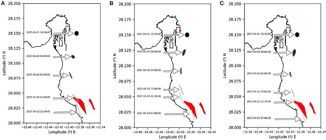
Figure 6. Simulations of the evolution of the spill in the neighborhood of the accident location, according to the three models. (A) IBI; (B) CST; (C) PRT. Evaporation is represented by the degradation of the gray scale. The red color marks the position of accident and the observed spill on the 23rd April at 7:00 a.m.

3.1. The Dynamical System Perspective

A comparison of the transport processes induced by the different models requires a further step than just a contrast between individual trajectories. This can be carried out by means of applying Poincaré's idea of seeking geometrical structures in the phase space of the dynamical system described in Equation (3) that are responsible for organizing particle trajectories schematically into regions corresponding to qualitatively distinct dynamical behaviors. This approach brings an interesting new perspective into this problem. Thereby, the global behavior of particle trajectories on the ocean surface can be understood through a template (skeleton) formed by geometrical structures that organize flow trajectories into different ocean regions. These structures are known in the literature as Lagrangian Coherent Structures (LCS), which provide a robust way to compare transport features between velocity datasets. This is due to the fact that the geometry of LCS is preserved even for not so small velocity perturbations (Haller and Yuan, 2000). In this way, works such as (de la Cámara et al., 2010), compare transport across the stratospheric polar vortex in the atmosphere due to different models. It shows that the comparison of individual trajectories is not a robust test to quantify transport features in stratospheric datasets, while LCS are.

An essential ingredient of the geometrical structures associated with LCS are hyperbolic trajectories characterized by high contraction and expansion rates. Directions of contraction and expansion define, respectively, stable and unstable directions (García-Garrido et al., 2016; Balibrea-Iniesta et al., 2019). Of particular interest to our study are hyperbolic trajectories located on the coastline in what is known as a detachment configuration. Under this configuration, which is illustrated in Figure 7, material on the coast is ejected into the ocean as shown by the successive green blobs. This configuration is related to the phenomena of flow separation. The presence of these hyperbolic trajectories close to the “Nelson Mandela” dike implies a higher risk of any spill event in such a location, because diesel fuel poured into the sea close to a detachment trajectory flows away, increasing the probability of affecting critical areas as those marked in Figure 1.

FIGURE 7

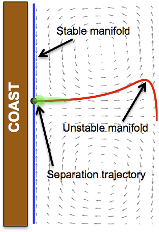
Figure 7. Sketch of a hyperbolic trajectory in a detachment or separation configuration. Successive green blobs separate from the coast flowing into the ocean.

Computing the geometrical skeleton formed by the stable and unstable manifolds of hyperbolic trajectories in the described ocean models requires additional mathematical techniques that we discuss next. To this end, we use a tool known as Lagrangian descriptors (Mendoza and Mancho, 2010; Mancho et al., 2013; Lopesino et al., 2017) that has been successfully applied in similar studies (García-Garrido et al., 2015, 2016). This tool is based on the construction of a scalar function that we call M, which is defined as follows (Madrid and Mancho, 2009):

$\begin{array}{ll}M({\text{x}}_0,t_0,\tau )={\displaystyle {\int }_{t_0-\tau }^{t_0+\tau }}||\text{v}(\text{x}(t),t)||dt,& (6)\end{array}$

where ||·|| stands for the modulus of the velocity vector. At a given time t₀, the function M(x₀, t₀, τ) measures the arclength traced by the trajectory starting at x₀ = x(t₀) as it evolves forward and backward in time for a time interval τ. Notice that we can split the computation of function M into its forward and backward contributions separately. This is important because forward integration provides information about the stable manifolds (repelling LCSs), while backward integration highlights the structure of unstable manifolds (attracting LCSs). Moreover, if we plot in the same figure the sum of both contributions, we can easily locate hyperbolic trajectories at the intersections of the stable and unstable manifolds. In fact, it can be shown that the scalar field provided by the computation of function M, when calculated over a grid of initial conditions, reveals the stable and unstable manifolds on the ocean surface at locations where the output values change abruptly, that is, at places where the gradient of the scalar field is very large. Figure 8 displays the calculation of M in the vicinity of the crash point using the CST model in the Port of La Luz coastal area. The pattern displayed by the function M has been computed for an integration period of τ = 3 days. In Figure 8, stable and unstable manifolds are emphasized, respectively, by the red and blue tones that enhance the “singular features” highlighted in the scalar field as a result of high gradient values. In this panel, a hyperbolic trajectory is visible as a point in a detachment configuration, similar to the one sketched in Figure 8. This trajectory is very close to the ferry crash point in the “Nelson Mandela” dike, which increases the riskiness of the region due to the dispersion of the spilled diesel fuel.

FIGURE 8

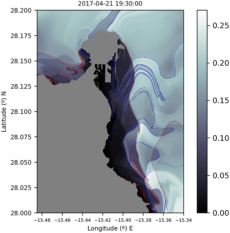
Figure 8. The Lagrangian skeleton of the CST model on the 21 April 2017 at 19:30h calculated with function M using τ = 3 days. LCSs are highlighted by the intricate curves in gray at the background, where there is a sharp change in the scalar field values of the function. Red lines are marked to emphasize the locations of the unstable manifolds (attracting LCSs), while blue lines depict the stable manifolds (repelling LCSs).

Figure 9 displays the M function for τ = 5 days. It highlights the LCSs for the three models at the time of the accident. This allows a straightforward qualitative comparison of the transport mechanisms produced by all models. The IBI and CST models present different patterns, however both show a detachment configuration as the one displayed in Figure 7. This confirms that both models will predict a southwards evolution of any spill in the neighborhood of the accident point. This is so because in both cases the unstable manifold follows that orientation. As expected, the PRT and CST models present very similar LCSs features. A comparison between Figures 8, 9B show that as τ is increased in the computation of the M function, this produces a richer and more intricate LCS skeleton, since we are incorporating more information about the history of particle trajectories as they evolve in time for longer periods.

FIGURE 9

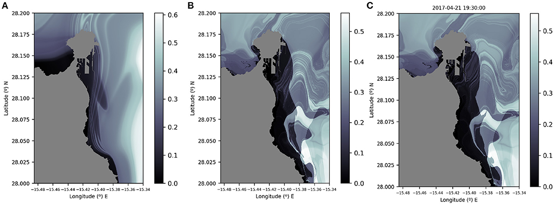
Figure 9. The Lagrangian skeleton as displayed by the function M computed for τ = 5 days on the 21 April 2017 at 19:30 h. LCSs are highlighted by the intricate curves in gray at the background, where there is a sharp change in the scalar field values of the function. (A) Results for the IBI model; (B) results for the CST model; (C) results for the PRT model. All three models display a detachment configuration.

The stable and unstable manifolds highlighted in Figure 9 are time dependent dynamical barriers that fluid parcels cannot cross. Fluid parcels tend to become aligned, for large enough transition time intervals, with unstable manifolds, which are attracting material curves that adopt convoluted shapes. This is true no matter what the initial position of the spill is. Supplementary Videos 1, 2 confirm this point. These movies show the evolution of several fluid blobs placed at different initial positions. At later times, all blobs are elongated and aligned with the unstable structures. This is the case, both for fluid parcels evolving according to the IBI model (Supplementary Video 1) and to the CST model (Supplementary Video 2). Similarly, but going backwards in time, blob particles align along repelling material curves, the stable manifolds, which also may be very intricate in shape. In forward time, stable manifolds represent the transition pathways toward the unstable manifolds.

3.2. Uncertainty Quantification

The Lagrangian geometrical structures computed for the PRT, CST, and IBI models allowed for a qualitative comparison among them, since they enhance similar features in what regards the presence of a separation or detachment trajectory on the coast close to the “Nelson Mandela” dike. This is a particular hyperbolic configuration that pushes material out of the coast. The flow evolution in the neighborhood of any hyperbolic trajectory is characterized by high expansion and contraction rates, which always are intrinsically related to uncertainties in the evolution. The outputs of the PRT and CST models, as already discussed, are barely distinguishable in the event scale. This is because the main differences in the circulation patterns are within the harbor. The analyzed spill was rapidly advected outside the harbor, where the solutions of both models are identical. Consequently, the very high resolution model would provide further insights only in those spills whose trajectories intersect the harbor waters.

In this section, we quantify the differences between the transport outputs by the CST and IBI models with respect to the position of the observed purple spill, which is considered a target, a “ground truth” that should be recovered by the model (see Figure 6). In order to achieve this, we have selected a number of positions in the neighborhood of the “Nelson Mandela” dike, which are centered within each grid element displayed in Figures 10A,B. The evolution of blobs of identical initial radius (0.0035°) from all those positions is different due to the chaotic nature of transport in this setting. After a time interval from the initial time, these blobs evolve and distort while they approach the target observed spill. The calculation of uncertainties associated to each grid element, is based on an error metric that considers the distance between the centroid of the simulated slick (c_m) at a given time t^* and the centroid of the ground value slick (c_g), i.e,

$\begin{array}{ll}e(t^{*})=||{\text{c}}_m(t^{*})-{\text{c}}_g||,& (7)\end{array}$

where ||·|| is the modulus of the vector. The centroid of a finite set of N points ${\left\{{\text{x}}_k\right\}}_{k\in \mathbb{N}}\in {ℝ}^n$ (n = 2 in this setting) is defined as:

$\begin{array}{ll}\text{c}=\frac{1}{N}{\displaystyle \sum _{k=1}^N}{\text{x}}_k,& (8)\end{array}$

where x_k are the (lon, lat) coordinates that define the contour of the slick in an equirectangular projection. Based on this error metric, the uncertainty of the model in a given grid element is computed starting on the 21st of April 2017, at time 7:30 p.m., from a circular contour centred on the grid with a radius of 0.0035°. Then the set of errors e_i defined as in Equation (7) are considered for a sample of times t_i, where i = 1…7, within a 3 h interval centred on the 23rd of April at 7:00 a.m., when the satellite image is taken. Finally, the minimum value of e_i in this set is taken as the representative error for each grid element. Results in a mesh next to the crash point are displayed in Figure 10. The error is given in degrees that can be easily transformed into kilometers. Grid elements of Figures 10A,B are colored in a different tone depending on this distance. The color scale is marked in the figure. It is evident that uncertainties, which are related to errors in the displacement, are greater for the IBI model than for the high resolution CST model. Using the regional solution the average error obtained is 0.07° (around 8 km), whereas using the coastal model solution the error is 0.03° (around 3 km). La Luz CST model errors are a factor 2.5 lower than the IBI model errors in good agreement with grid sizes differences.

FIGURE 10

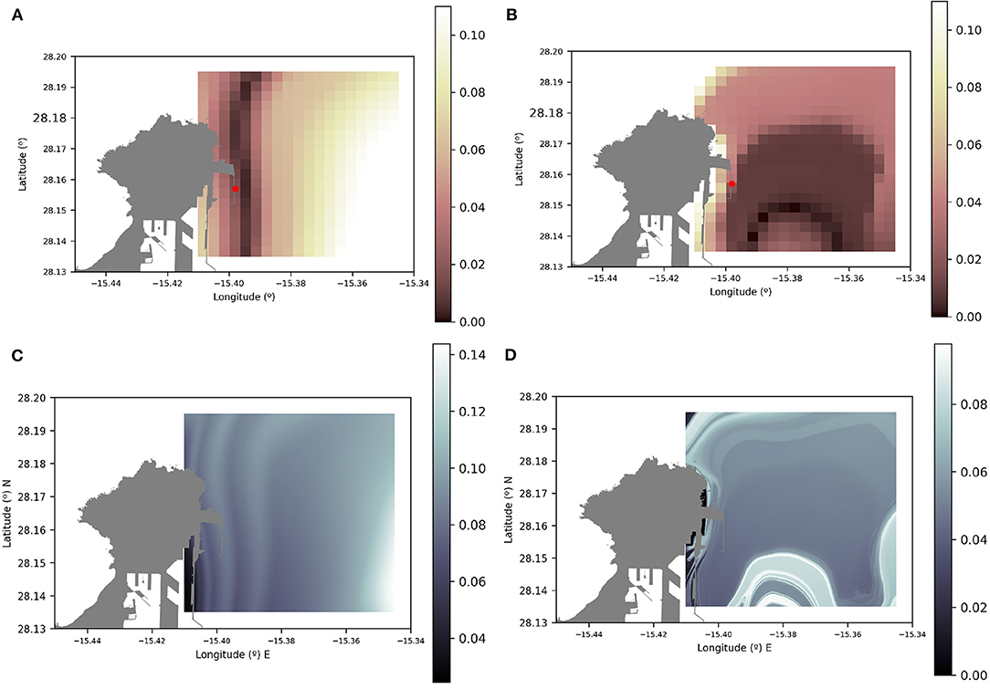
Figure 10. (A,B): A quantitative measure of uncertainty based on blob initial positions and representative errors measured as distances to the target “ground truth” spill. Higher colormap values correspond to larger errors or uncertainties. The accident location is marked with a red spot. (A) Uncertainties associated to the IBI model; (B) uncertainties associated to the high resolution La Luz model. (C,D): Representation of the forward integrated M function for τ = 3 days highlighting the stable manifolds. (C) Stable manifolds associated to the IBI model; (D) stable manifolds associated to the CST model.

Differences in the uncertainty distributions are visible from Figures 10A,B. IBI uncertainties are more significant in the right side of the mesh, while CST uncertainties are higher in the upper side. Figures 10C,D, show for the IBI and CST models, respectively, in the same area, the structure of the stable manifolds as highlighted by the M function. Indeed, stable manifolds are displayed by formula (6) when the integration interval is a forward time integration, i.e., (t₀ − τ, t₀ + τ) is replaced by (t₀, t₀+τ). Similarities between patterns in Figures 10A,C and those in Figures 10B,D are remarkable. Uncertainties seem to reach minimum values along the stable manifolds. Indeed, as explained before, and is visible from Supplementary Videos 1, 2, blobs on the stable manifolds rapidly travel toward the unstable manifolds, which in turn are the attracting material curves toward which all fluid parcels evolve. In this case both IBI and CST models have their unstable manifolds aligned with the observed spill, on the 23rd of April 2017.

4. Conclusions

In this paper we have analyzed how emerging tools in coastal areas such as available very high resolution hydrodynamic models and remote sensing images from satellite, are able to provide accurate responses to the management of pollution events in port areas. In particular, the collision event of the passenger ferry “Volcán de Tamasite” in La Luz Port on April 2017 is discussed.

Very good agreement is reported between Sentinel 1 radar images and spill evolution models based on velocity fields obtained from the CMEMS IBI regional product and from the two specific model solutions: the coastal one, CST, covering waters along the eastern coast of the Gran Canaria Island and; the highest resolution one, PRT, focused exclusively in the nearby waters of Puerto de la Luz. These downstream were developed by PdE, in the framework of the IMPRESSIVE project, to downscale the CMEMS regional solution.

The evolution of the spill is implemented with contour advection algorithms that are able to track very efficiently the whole area where the fuel is extended. This is so because the algorithm is capable of self-regulating the number of fluid parcels on the contour, to ensure an accurate representation of distortions at all times. Transformation process are caused by evaporation and are expressed by means of a degradation in the gray tone representing the spill.

Transport process describing the spill evolution under the IBI, CST, and PRT models have been analyzed from the dynamical systems perspective. This perspective has allowed a qualitative comparison among them and has highlighted a similar transport scenario in the three models, in which the spreading of the fuel is controlled by the presence of a hyperbolic trajectory attached to the coast, close the “Nelson Mandela” dike, in a detachment configuration. This configuration pushes waters along the coast out into the sea. In this framework, attracting material surfaces, also called invariant unstable manifolds, are identified. Passive scalars, and fuel behaves like them, become aligned along them.

A quantitative comparison of the transport outputs by the CST and IBI models has been implemented. For blobs in a neighborhood of the accident point, an estimation of the uncertainty is provided by measuring errors or distances between simulated and observed spills. The average uncertainty is found to be lower for the CST than for the IBI model. Connections between stable manifolds and the uncertainty field have been discussed. It is observed that for both models, minimum values of the uncertainty field are aligned along stable manifolds. This is congruent with the fact that stable manifolds are optimal transport routes toward the unstable manifolds and that all models consistently present unstable manifolds aligned with the observed spill.

Summarizing, counting with a coastal downstream service focused on downscaling the regional CMEMS solution by means of a higher resolution nested model is proved to be a positive approach. In particular, high resolutions models decrease uncertainties in oil spill predictions. This confirms that high resolutions tools have the potential to be effective contributors to the decision-making processes carried out by the emergency services in the real-time management of oil spills.

Data Availability Statement

The raw data supporting the conclusions of this article will be made available by the authors, without undue reservation.

Author Contributions

GG-S did Figures 1, 4–6, 8–10. AM did Figure 7. GG-S and AM contributed to sections 1, 2.3, 3, 3.1, 3.2, and 4. VG-G contributed to sections 3, 3.1, and 4. SW contributed to sections 1, 3, 3.1, 3.2, and 4. AR and JC did the Figure 2 and contributed to sections 1, 2.1, 3, and 4. BP-G, EÁ-F, MS, and MG-L did the Figure 3 and contributed to sections 1, 2.2, 3, and 4. All authors wrote the paper.

Funding

The authors acknowledge support from IMPRESSIVE, a project funded by the European Union's Horizon 2020 research and innovation programme under grant agreement No 821922. The authors acknowledge support of the publication fee by the CSIC Open Access Publication Support Initiative through its Unit of Information Resources for Research (URICI). SW acknowledges the support of ONR Grant No. N00014-01-1-0769.

Conflict of Interest

The authors declare that the research was conducted in the absence of any commercial or financial relationships that could be construed as a potential conflict of interest.

Supplementary Material

The Supplementary Material for this article can be found online at: https://www.frontiersin.org/articles/10.3389/fmars.2020.605804/full#supplementary-material

Supplementary Video 1. The movie shows the evolution of several oil slicks overlapped with the Lagrangian Coherent Structures obtained from Copernicus IBI ocean currents (IBI model) during the Volcan de Tamasite event in April 2017 in Gran Canaria area. Oil slicks are eventually aligned with the unstable manifolds.

Supplementary Video 2. The movie shows the evolution of several oil slicks overlapped with the Lagrangian Coherent Structures obtained from Puertos del Estado ocean currents (CST model) during the Volcan de Tamasite event in April 2017 in Gran Canaria area. Oil slicks are eventually aligned with the unstable manifolds.

References

Amo, A., Reffray, G., Sotillo, M. G., Aznar, R., and Guihou, K. (2020). PRODUCT USER MANUAL Atlantic -Iberian Biscay Irish- Ocean Physics Analysis and Forecast Product: IBI_ANALYSIS_FORECAST_PHYS_005_001. Available online at: https://resources.marine.copernicus.eu/documents/PUM/CMEMS-IBI-PUM-005-001.pdf

Google Scholar

Aznar, R., Sotillo, M., Cailleau, S., Lorente, P., Levier, B., Amo-Baladrón, A., et al. (2016). Strengths and weaknesses of the CMEMS forecasted and reanalyzed solutions for the Iberia-Biscay-Ireland (IBI) waters. J. Mar. Syst. 159, 1–14. doi: 10.1016/j.jmarsys.2016.02.007

CrossRef Full Text | Google Scholar

Balibrea-Iniesta, F., Xie, J., García-Garrido, V. J., Bertino, L., Mancho, A. M., and Wiggins, S. (2019). Lagrangian transport across the upper Arctic waters in the Canadian Basin. Q. J. R. Meteorol. Soc. 145, 76–91. doi: 10.1002/qj.3404

CrossRef Full Text | Google Scholar

Bengtsson, L., Andrae, U., Aspelien, T., Batrak, Y., Calvo, J., de Rooy, W., et al. (2017). The HARMONIE-AROME Model Configuration in the ALADIN-HIRLAM NWP system. Mon. Weather Rev. 145, 1919–1935. doi: 10.1175/MWR-D-16-0417.1

CrossRef Full Text | Google Scholar

Butler, J. N. (1976). “Transfer of petroleum residues from sea to air: evaporative weathering,” in Marine Pollutant Transfer eds H. L. Windom and R. A. Duce (Toronto, ON: Lexington Books), 201–212.

Google Scholar

Capet, A., Fernández, V., She, J., Dabrowski, T., Umgiesser, G., Staneva, J., et al. (2020). Operational modeling capacity in European seas–An EuroGOOS perspective and recommendations for improvement. Front. Mar. Sci. 7:129. doi: 10.3389/fmars.2020.00129

CrossRef Full Text | Google Scholar

Cartwright, J. H. E., Feudel, U., Károlyi, G., de Moura, A., Piro, O., and Tél, T. (2010). “Dynamics of finite-size particles in chaotic fluid flows,” in Non-linear Dynamics and Chaos: Advances and Perspectives eds M. Thiel, J. Kurths, M. C. Romano, G. Klyi, and A. Moura (Berlin; Heidelberg: Springer), 51–87. doi: 10.1007/978-3-642-04629-2_4

CrossRef Full Text | Google Scholar

Cheng, Y., Li, X., Xu, Q., Garcia-Pineda, O., Andersen, O. B., and Pichel, W. G. (2011). SAR observation and model tracking of an oil spill event in coastal waters. Mar. Pollut. Bull. 62, 350–363. doi: 10.1016/j.marpolbul.2010.10.005

PubMed Abstract | CrossRef Full Text | Google Scholar

CIAIM (2018). Informe de colision del buque RO/PAX VOLCÁN DE TAMASITE contra el dique Nelson Mandela del puerto de Las Palmas de Gran Canaria, el 21 de abril de 2017. CIAIM-05/2018. Ministerio de Fomento. Gobierno de Espana. 27. Available online at: https://www.mitma.gob.es/recursos_mfom/comodin/recursos/ic_05-2018_vtamasite_web.pdf

Google Scholar

De Dominicis, M., Bruciaferri, D., Gerin, R., Pinardi, N., Poulain, P., Garreau, P., et al. (2016). A multi-model assessment of the impact of currents, waves and wind in modelling surface drifters and oil spill. Deep Sea Res. II Top. Stud. Oceanogr. 133, 21–38. doi: 10.1016/j.dsr2.2016.04.002

CrossRef Full Text | Google Scholar

De Dominicis, M., Pinardi, N., Zodiatis, G., and Lardner, R. (2013). MEDSLIK-II, a Lagrangian marine surface oil spill model for short-term forecasting - Part 1: theory. Geosci. Model Dev. 6, 1851–1869. doi: 10.5194/gmd-6-1851-2013

CrossRef Full Text | Google Scholar

de la Cámara, A., Mechoso, C. R., Ide, K., Walterscheid, R., and Schubert, G. (2010). Polar night vortex breakdown and large-scale stirring in the southern stratosphere. Clim. Dyn. 35, 965–975. doi: 10.1007/s00382-009-0632-6

CrossRef Full Text | Google Scholar

Dritschel, D. G. (1989). Contour dynamics and contour surgery: numerical algorithms for extended, high-resolution modelling of vortex dynamics in two-dimensional, inviscid, incompressible flows. Comput. Phys. Rep. 10, 77–146. doi: 10.1016/0167-7977(89)90004-X

CrossRef Full Text | Google Scholar

Fingas, M. (2014). “Oil and petroleum evaporation,” in Handbook of Oil Spill Science and Technology ed M. Fingas (Hoboken, NJ: John Wiley & Sons), 205–223. doi: 10.1002/9781118989982.ch7

CrossRef Full Text | Google Scholar

García-Garrido, V. J., Mancho, A. M., Wiggins, S., and Mendoza, C. (2015). A dynamical systems approach to the surface search for debris associated with the disappearance of flight MH370. Nonlin. Process. Geophys. 22, 701–712. doi: 10.5194/npg-22-701-2015

CrossRef Full Text | Google Scholar

García-Garrido, V. J., Ramos, A., Mancho, A. M., Coca, J., and Wiggins, S. (2016). A dynamical systems perspective for a real-time response to a marine oil spill. Mar. Pollut. Bull. 112, 201–210. doi: 10.1016/j.marpolbul.2016.08.018

PubMed Abstract | CrossRef Full Text | Google Scholar

Grifoll, M., Jordá, G., Sotillo, M. G., Ferrer, L., Espino, M., Sánchez-Arcilla, A., et al. (2012). Water circulation forecasting in Spanish harbours. Sci. Mar. 76, 45–61. doi: 10.3989/scimar.03606.18B

CrossRef Full Text | Google Scholar

Haller, G., and Yuan, G. (2000). Lagrangian coherent structures and mixing in two-dimensional turbulence. Phys. D 147, 352–370. doi: 10.1016/S0167-2789(00)00142-1

CrossRef Full Text | Google Scholar

Large, W. G., and Yeager, S. (2004). Diurnal to Decadal Global Forcing for Ocean and Sea-Ice Models: The Data Sets and Flux Climatologies. University Corporation for Atmospheric Research.

Google Scholar

Lekien, F., Coulliette, C., Mariano, A., Ryan, E., Shay, L., Haller, G., et al. (2005). Pollution release tied to invariant manifolds: a case study for the coast of Florida. Phys. D 210, 1–20. doi: 10.1016/j.physd.2005.06.023

CrossRef Full Text | Google Scholar

Lopesino, C., Balibrea-Iniesta, F., García-Garrido, V. J., Wiggins, S., and Mancho, A. M. (2017). A theoretical framework for lagrangian descriptors. Int. J. Bifurcat. Chaos 27:1730001. doi: 10.1142/S0218127417300014

CrossRef Full Text | Google Scholar

Lorente, P., Sotillo, M. G., Amo-Baladrón, A., Aznar, R., Levier, B., Aouf, L., et al. (2019). “The NARVAL software toolbox in support of ocean models skill assessment at regional and coastal scales,” in Proceedings of the 19th International Conference on Computational Science (Faro). doi: 10.1007/978-3-030-22747-0_25

CrossRef Full Text | Google Scholar

Madec, G. NEMO Team (2019). Nemo ocean engine. Available online at: https://www.nemo-ocean.eu/doc/

Google Scholar

Madrid, J. A. J., and Mancho, A. M. (2009). Distinguished trajectories in time dependent vector fields. Chaos 19:013111. doi: 10.1063/1.3056050

PubMed Abstract | CrossRef Full Text | Google Scholar

Mancho, A., Small, D., and Wiggins, S. (2004). Computation of hyperbolic trajectories and their stable and unstable manifolds for oceanographic flows represented as data sets. Nonlinear Proc. Geoph 11, 17–33. doi: 10.5194/npg-11-17-2004

CrossRef Full Text | Google Scholar

Mancho, A., Small, D., Wiggins, S., and Ide, K. (2003). Computation of stable and unstable manifolds of hyperbolic trajectories in two-dimensional, aperiodically time-dependent vectors fields. Phys. D 182, 188–122. doi: 10.1016/S0167-2789(03)00152-0

CrossRef Full Text | Google Scholar

Mancho, A. M., Small, D., and Wiggins, S. (2006). A tutorial on dynamical systems concepts applied to Lagrangian transport in oceanic flows defined as finite time data sets: theoretical and computational issues. Phys. Rep. 437, 55–124. doi: 10.1016/j.physrep.2006.09.005

CrossRef Full Text | Google Scholar

Mancho, A. M., Wiggins, S., Curbelo, J., and Mendoza, C. (2013). Lagrangian descriptors: a method for revealing phase space structures of general time dependent dynamical systems. Commun. Nonlinear Sci. Num. Simul. 18, 3530–3557. doi: 10.1016/j.cnsns.2013.05.002

CrossRef Full Text | Google Scholar

Marta-Almeida, M., Ruiz-Villarreal, M., Pereira, J., Otero, P., Cirano, M., Zhang, X., et al. (2013). Efficient tools for marine operational forecast and oil spill tracking. Mar. Pollut. Bull. 71, 139–151. doi: 10.1016/j.marpolbul.2013.03.022

PubMed Abstract | CrossRef Full Text | Google Scholar

Maxey, M. R., and Riley, J. J. (1983). Equation of motion for a small rigid sphere in a nonuniform flow. Phys. Fluids 26:883. doi: 10.1063/1.864230

PubMed Abstract | CrossRef Full Text | Google Scholar

McIlroy, J. W., Smith, R. W., and McGuffin, V. L. (2018). Fixed- and variable-temperature kinetic models to predict evaporation of petroleum distillates for fire debris applications. Separations 5, 1–19. doi: 10.3390/separations5040047

CrossRef Full Text | Google Scholar

Mendoza, C., and Mancho, A. M. (2010). The hidden geometry of ocean flows. Phys. Rev. Lett. 105:038501. doi: 10.1103/PhysRevLett.105.038501

PubMed Abstract | CrossRef Full Text | Google Scholar

Monroy, P. (2019). Doctoral thesis: Lagrangian studies of sedimentation and transport. Impact on marine ecosystems. Universitat de les Illes Balears. Available online at: https://ifisc.uib-csic.es/es/publications/lagrangian-studies-of-sedimentation-and-transport/

Google Scholar

Monroy, P., Hernández-Garcia, E., Rossi, V., and López, C. (2017). Modeling the dynamical sinking of biogenic particles in oceanic flow. Nonlin. Process. Geophys. 24, 293–305. doi: 10.5194/npg-24-293-2017

CrossRef Full Text | Google Scholar

Montero, A. R. (2017). La reducción de la mancha de gasoil un 80% permite abrir las ocho playas. La Provincia. Available online at: https://www.laprovincia.es/las-palmas/2017/04/25/reduccion-mancha-gasoil-80-permite-9723032.html

Google Scholar

Olascoaga, M. J., and Haller, G. (2012). Forecasting sudden changes in environmental pollution patterns. Proc. Natl. Acad. Sci. U.S.A. 109, 4738–4743. doi: 10.1073/pnas.1118574109

PubMed Abstract | CrossRef Full Text | Google Scholar

Pisano, A., Bignami, F., and Santoleri, R. (2015). Oil spill detection in glint-contaminated near infrared modis imagery. Remote Sens. 7, 1112–1134. doi: 10.3390/rs70101112

CrossRef Full Text | Google Scholar

Shapiro, R. (1970). Smoothing, filtering, and boundary effects. Rev. Geophys. 8, 359–387. doi: 10.1029/RG008i002p00359

CrossRef Full Text | Google Scholar

Shchepetkin, A. F., and McWilliams, J. C. (2005). The regional oceanic modeling system (ROMS): a split-explicit, free-surface, topography-following-coordinate oceanic model. Ocean Modell. 9, 347–404. doi: 10.1016/j.ocemod.2004.08.002

CrossRef Full Text | Google Scholar

Song, Y., and Haidvogel, D. (1994). A semi-implicit ocean circulation model using a generalized topography-following coordinate system. J. Comput. Phys. 115, 228–244. doi: 10.1006/jcph.1994.1189

CrossRef Full Text | Google Scholar

Sotillo, M., Levier, B., Lorente, P., Guihou, K., and Aznar, R. (2020a). CMEMS Quality Information Document for the CMEMS IBI Product: IBI_ANALYSIS_FORECAST_PHYS_005_001. Available online at: https://resources.marine.copernicus.eu/documents/QUID/CMEMS-IBI-QUID-005-001.pdf

Google Scholar

Sotillo, M. G., Cailleau, S., Lorente, P., Levier, B., Aznar, R., Reffray, G., et al. (2015). The MyOcean IBI Ocean Forecast and Reanalysis Systems: operational products and roadmap to the future Copernicus Service. J. Operat. Oceanogr. 8, 63–79. doi: 10.1080/1755876X.2015.1014663

CrossRef Full Text | Google Scholar

Sotillo, M. G., Cerralbo, P., Lorente, P., Grifoll, M., Espino, M., Sanchez-Arcilla, A., et al. (2020b). Coastal ocean forecasting in Spanish ports: the SAMOA operational service. J. Operat. Oceanogr. 13, 37–54. doi: 10.1080/1755876X.2019.1606765

CrossRef Full Text | Google Scholar

TeldeActualidad/EFE (2017). La punta de la mancha, de 13 km. de largo, ya esta a la altura de La Garita pero a 1.000 metros de la costa. Telde Actualidad, Available online at: https://www.teldeactualidad.com/hemeroteca/noticia/medioambiente/2017/04/23/2402.html

Google Scholar

Vanhellemont, Q. (2019). Remote sensing of environment adaptation of the dark spectrum fi fitting atmospheric correction for aquatic applications of the Landsat and Sentinel-2 archives. Remote Sens. Environ. 225, 175–192. doi: 10.1016/j.rse.2019.03.010

CrossRef Full Text | Google Scholar

Warner, J. C., Sherwood, C. R., Arango, H. G., and Signell, R. P. (2005). Performance of four turbulence closure models implemented using a generic length scale method. Ocean Modell. 8, 81–113. doi: 10.1016/j.ocemod.2003.12.003

CrossRef Full Text | Google Scholar

Wiggins, S. (2005). The dynamical systems approach to Lagrangian transport in oceanic flows. Annu. Rev. Fluid Mech. 37, 295–328. doi: 10.1146/annurev.fluid.37.061903.175815

CrossRef Full Text | Google Scholar

Xu, Q., Li, X., Wei, Y., Tang, Z., Cheng, Y., and Pichel, W. G. (2013). Satellite observations and modeling of oil spill trajectories in the Bohai Sea. Mar. Pollut. Bull. 71, 107–116. doi: 10.1016/j.marpolbul.2013.03.028

PubMed Abstract | CrossRef Full Text | Google Scholar