Multiple Metrics of Temperature, Light, and Water Motion Drive Gradients in Eelgrass Productivity and Resilience

Introduction

Coastal vegetated marine habitats, such as seagrass, seaweed, and salt marsh ecosystems are vulnerable to changing environmental conditions and anthropogenic stressors, leading to widespread declines over the past several decades (Lotze et al., 2006; Waycott et al., 2009; Krumhansl et al., 2016). Marine macrophytes enhance secondary production through the provision of habitat and food (Krumhansl and Scheibling, 2012; Wong, 2018), and play a significant role in carbon and nutrient cycling and storage (Fourqurean et al., 2012), thereby providing billions of dollars annually in ecosystem services to humans (Barbier et al., 2011; Filbee-Dexter and Wernberg, 2018). Understanding how environmental conditions impact the functioning of marine ecosystems, as well as their susceptibility to disturbance, is critical for decision making processes related to nearshore conservation and management (Unsworth et al., 2015). In particular, identifying the environmental conditions under which marine macrophyte communities remain resilient within the context of climate change is critical for maximizing the effectiveness of conservation strategies.

Research into the response of seagrasses to environmental change has evolved from manipulative studies of single stressors to factorial experiments of multiple stressors acting in synergy (e.g., Gao et al., 2017; Moreno-Marin et al., 2018). However, the physiological and ecological performance of seagrasses are influenced by a suite of environmental variables, including light, temperature, sediment properties, salinity, nutrients, and water motion (Koch, 2001; Lee et al., 2007), the interactive effects of which are difficult to simulate in an experimental setting. An alternative approach is to investigate emergent properties of ecosystems, which represent the cumulative effects of the full suite of relevant environmental variables and associated processes over varying time scales (Odum and Barrett, 1971). Further, investigating emergent properties of seagrass communities at sites spanning environmental gradients and levels of stress can provide insights into how these ecosystems respond to environmental change, and the relative importance of different environmental variables for driving a biological response.

Previous work has shown that seagrass bioindicators (or traits) can be used to understand the nature of seagrass change, since indicator responses vary with the type and duration of exposure to stress, and depend on the physiological and ecological processes impacted (McMahon et al., 2013; Wong et al., 2020a). Measuring suites of bioindicators over environmental gradients can be an effective strategy to capture the range of possible biological responses to varying environmental conditions. Changes in primary production, a key ecosystem function, in relation to environmental stressors has been assessed using measures of photosynthetic performance, as well as emergent properties of growth and acclimation to low and high light conditions, including tissue biochemistry, plant morphology, and biomass (Martínez-Crego et al., 2008; McMahon et al., 2013; Gao et al., 2017; Hammer et al., 2018; Bertelli et al., 2020). Seagrass resilience is also impacted by processes that reduce the capacity for seagrasses to resist and recover from disturbance, and is measured, in part, by factors such as the production of defensive compounds, the capacity to build carbohydrate reserves, and the ability to recover from habitat disturbance through asexual vegetative growth and sexual reproduction (Unsworth et al., 2015).

Previous research has provided insight into how varying light conditions, water current speeds, wave exposures, and sediment characteristics impact seagrass ecosystem properties. Light stress is considered one of the primary factors impacting seagrass ecosystem productivity and resilience to disturbance (Lee et al., 2007; Ochieng et al., 2010; Lefcheck et al., 2017; Wong et al., 2020b), and the depth distribution of seagrasses are largely determined by light availability (Krause-Jensen et al., 2011). Light availability is influenced indirectly by sediment properties, as finer sediments are more easily re-suspended than coarser sediments, leading to increased turbidity and reduced light. Fine sediments are also linked to high concentrations of hydrogen sulfide, which are toxic to seagrass plants (Goodman et al., 1995; Pérez et al., 2007; Krause-Jensen et al., 2011). High water motion can increase seagrass production by thinning the diffusive boundary layer and increasing carbon uptake (Koch, 2001), reduce epiphytic growth (Lavery et al., 2007), and can be associated with cooler temperatures and clearer waters as a result of high flushing rates. High water motion also influences bed patchiness on a landscape scale through physical disturbance (Fonseca and Bell, 1998; Fonseca et al., 2002).

Growing evidence for a rapidly changing climate has increased the emphasis on temperature effects on seagrasses (Short and Neckles, 1999; Campbell et al., 2006; Rasheed and Unsworth, 2011; Strydom et al., 2020). Initial studies identified optimal temperature thresholds for productivity and survival (Biebl and McRoy, 1971; Evans et al., 1986; Marsh et al., 1986), and documented seasonal changes in productivity, biomass, and survival in response to temperature and light in the field (Cabello-Pasini et al., 2003; Bostrom et al., 2004; Lee et al., 2005; Wong et al., 2013; Richardson et al., 2018). More recently, the focus has shifted to the impacts of extreme temperature events, as large-scale losses of seagrass have been documented in association with marine heat waves (Marbà and Duarte, 2010; Moore et al., 2014; Hammer et al., 2018; Saava et al., 2018; DuBois et al., 2019; Shields et al., 2019; Strydom et al., 2020). With this has come an awareness that changes to mean temperatures does not always cause the most dramatic biological responses as compared to temperature variability (George et al., 2018; Shields et al., 2019; Smale et al., 2019), leading to alternative ways in which temperature effects are characterized (e.g., warm water events, temperature variation, degree days) (Marbà and Duarte, 2010; Oliver et al., 2018).

Here, we investigate a suite of biological metrics for the temperate seagrass Zostera marina (eelgrass) in Nova Scotia, Canada that reflect emergent properties of plant functioning and resilience over environmental gradients, including temperature, light, water motion, and sediment properties. To understand the interactive effects of different forms of environmental change and disturbance, we evaluate the relative importance of different environmental metrics in driving spatial patterns in these emergent properties. To support a more detailed understanding of temperature effects on seagrass emergent properties, we also examine the relative importance of a variety of temperature metrics, including those that characterize the mean conditions, as well as temperature extremes and variability over different time scales. This work provides insight into the conditions necessary for seagrass resilience, and demonstrates the utility of a framework through which species-environment interactions can be assessed to provide information necessary for the conservation and management of coastal ecosystems.

Materials and Methods

Study Sites

Ten sites were selected along the Atlantic coast of Nova Scotia to represent the range of environmental conditions over which Zostera marina beds occur (Figure 1). Specifically, sites were chosen a priori to span the range of environmental gradients of temperature, light, sediment properties, and water motion (as influenced by tidal currents, wind, waves, depth, and slope) (Bakirman and Gumusay, 2020). Human impacts relating to coastal development and eutrophication were relatively low at all sites (Murphy et al., 2019). At six of the sites, two different locations were designated to capture within-site variation related to depth (termed “deep” and “shallow”; five sites) or dominant substrate (“sandy” and “muddy”; one site). Depth locations were chosen to characterize the largest differences in depth evident across extensive areas of each bed. Four sites did not have a large enough depth gradient to examine. Overall, sites ranged in depth from 0.9–6.2 m (mean depth at high tide) (Supplementary Table S1).

FIGURE 1

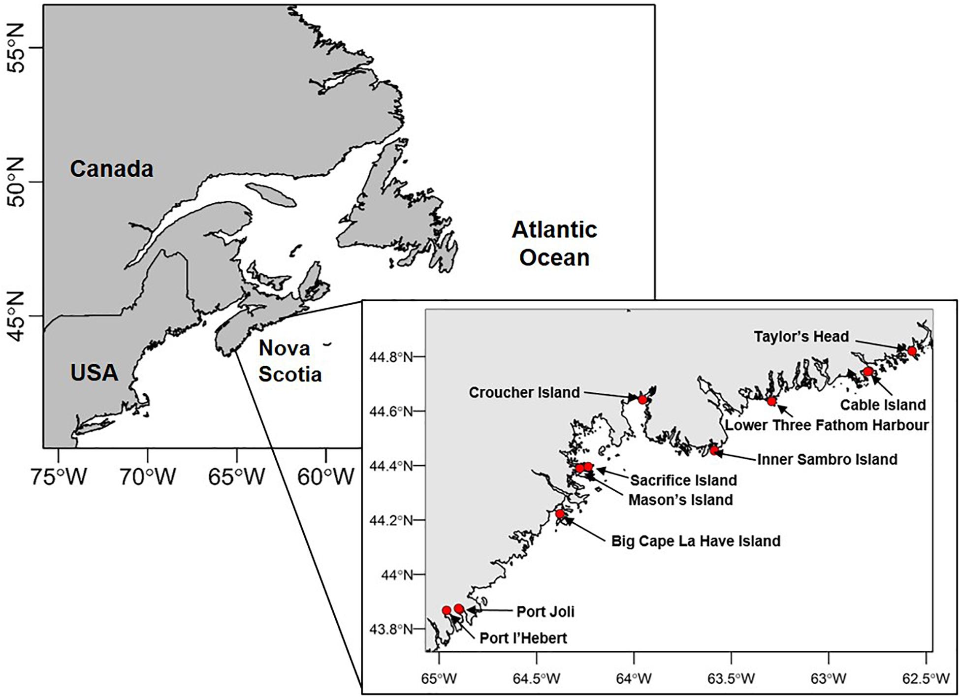
Figure 1. Study sites along the Atlantic coast of Nova Scotia, Canada.

At all sites and locations, a suite of biological and environmental measurements were taken to describe the status of the eelgrass bed and surrounding environment. All biological metrics were taken in July 2017 with the exception of bed patchiness. While some environmental measures (temperature, sediments, wave exposure) coincided with the biological sampling, by logistical necessity light, water currents and slope were measured the following year (June–September 2018). In spite of the time asynchrony, measurements captured the relative differences among sites, which are similar between years (Supplementary Table S3, M. Wong, unpublished data). We note that this study does not consider other biological variables (e.g., competition, herbivory, epiphyte fouling) that can impact eelgrass production and resilience.

Environmental Conditions

Temperature

Near-seabed temperature was recorded at 10-min intervals within eelgrass beds at all sites and locations from May/June 2017-April/May 2018 using HOBO tidbit temperature loggers (Onset Corp). At some sites, loggers were exposed at low tide, but these recordings were retained in the record because warm aerial temperatures are known to impact seagrasses (Kim et al., 2016), and these were in fact representative of the temperature experienced by plants at low tide. From the temperature time series, we calculated the mean, maximum, 95th percentile, and standard deviation for the year. As a heat wave metric, we then quantified the number of days above 23°C at each site, the mean optimal temperature for productivity of Zostera marina (Lee et al., 2007). We also characterized temperature variability over short (<36 h) and medium (36 h – 60 days) time scales using time series analysis as in Krumhansl et al. (2020), and computed the ratio of high (short time scale) to mid frequency temperature changes (HF:MF temperature variability) as an indication of the relative importance of changes in daily temperature from tides and cycles of heating and cooling versus those of storms and upwelling events in the temperature record. We also used the high frequency temperature time series to calculate the average range of temperatures over tidal and daily cycles (Krumhansl et al., 2020). Growing Degree Day (GDD) was calculated as a quantification of heat accumulation in a system (Neuheimer and Taggart, 2007) using 11°C as a base temperature, generated using the statistical method described by Yang et al. (1995) with no maximum temperature cap (see Krumhansl et al., 2020 for details). Note, we did not include minimum temperatures in our analysis because we found that the biological metrics correlated with HF:MF temperature variability were the same as those correlated with minimum temperatures, indicating that the low temperature effect on eelgrasses is more closely related to the range and variability of temperatures experienced than to the absolute minimum, which in some cases was well below 0°C due to logger exposure to the air. Note, the direction of the relationships between biological metrics and minimum temperature were inverse to those with HF:MF temperature variability, as higher temperature variability is correlated with a lower minimum temperature. Time series analyses were done using functions in the signal (Signal Developers, 2013), TSA (Chan and Ripley, 2012), astsa (Stoffer, 2017), and tseries (Trapletti and Hornik, 2018) packages in R (R Core Team, 2017).

Currents and Depth

Current speeds were recorded in burst samples every 10 min (20 samples per burst, 2 s intervals between samples) at each site using an electromagnetic current meter (Infinity-EM AEM, JFE Advantech), deployed < 1 m above bottom within the eelgrass bed for a 2–3-week period between June–September 2018. When sites contained deep and shallow locations, current meters were only deployed in the deep location due to logistical constraints (Sambro, Sacrifice, Croucher, Cable, Taylor’s Head). Current speed measurements were averaged across each burst, and then summarized by the mean, maximum, minimum, and standard deviation for each time series. Pressure sensors (HOBO Water Level Loggers, Onset Corp.) were deployed simultaneously with current meters and measured depth every 10 min. Mean depth at high tide was calculated by isolating local maxima within the dominant 12.42 h M₂ tidal cycle after smoothing with a harmonic regression, and averaging these depths across all high tides (Krumhansl et al., 2020).

PAR (Photosynthetically Active Radiation)

Downwelling irradiance (PAR: 400–700 nm) was recorded at 10-min intervals at each site and location using light sensors (DEFI2-L, JFE Advantech Co., Ltd.) deployed for 2–3 weeks periods between June and September 2018, coinciding with current meter and depth sensor deployments. Two PAR sensors were set at a fixed vertical distance from each other (0.5–1 m) and above the bottom (<0.5 m) in bare areas within the seagrass bed. Light attenuation coefficients were calculated from the two sets of light measurements using the Beer–Lambert law (Kirk, 2011) and averaged for each site and location. Mean and max PAR were also calculated using data recorded by the bottom light sensor.

Wave Exposure, Slope, and Sediment Properties

A relative index of wave exposure was calculated using a modification of the index by Keddy (1982) from wind data obtained from a centrally located Environment Canada weather station (Shearwater RCS, 44° 37′ 47′′ N, 63° 30′ 48′′ W) from January 2016 to December 2017 (Krumhansl et al., 2020). This time period was selected to provide a representative estimate of wave exposure over the 2 years period prior to and encompassing the field season when biological measures were taken. Fetch was calculated for each site and location using the fetch function in R (package fetchR, Seers, 2018).

Slope angle of the seagrass bed was estimated by measuring depth at 2 m increments along two or three, 50 m transects positioned perpendicular to the shore. The angle between successive 2 m intervals was calculated as the arctangent of the depth difference between sequential points, divided by the along bottom distance (Krumhansl et al., 2020). The resulting slope angles were averaged across sequential points to estimate overall slope angle for each site and location.

Sediment grain size distribution was determined in July 2017 using a wet sieve method as described in Wong et al. (2013). Percent fractions of gravel (≥2000 μm) and sand (64–2000 μm) were calculated from the dry mass of each fraction divided by the total dry mass and multiplied by 100. Percent fraction mud and silt was calculated as the total dry mass minus the dry mass of the gravel and sand fractions, divided by the total dry mass and multiplied by 100. Given that gravel was only present at a few sites and that mud/silt and sand fractions were highly collinear, only percent sand was used in the analyses.

Biological Metrics

Biological metrics were collected at all sites and locations. They were split into two categories: metrics of production, and metrics of resilience. Metrics of production included chlorophyll concentration, number of leaves, sheath length, length of the third oldest leaf (leaf 3), vegetative shoot density, and canopy height; while metrics of resilience included phenolic acid and rhizome water soluble carbohydrate (WSC) concentrations, leaf nitrogen content, reproductive shoot density, above to belowground biomass ratio, and eelgrass patch size and density. These groupings of variables spanned biological scales, from landscape to bed, as well as plant morphological and physiological properties.

Landscape and Bed Properties

Bed fragmentation at each field site was measured using five, 50 m × 1 m transects once between July and September 2018 by snorkelers or SCUBA divers. Transects were laid parallel to shore along a depth contour. Observers noted the dominant substrate cover at the start of each transect, defined as the sediment or macrophyte type occupying ≥50% of the bottom within a 1 × 1 m area encompassing the transect, and then swam along the transect recording each location (as distance along the transect) where bottom cover changed. Average eelgrass patch size was calculated as the average along-transect length of a patch (maximum 50 m), and patch density was calculated as the number of patches per transect.

Eelgrass plant and population characteristics were recorded at 10 haphazardly chosen sampling stations within each eelgrass bed in July 2017. Stations were at least 2 m from the bed edge and 10 – 15 m apart. At each station, canopy height was measured as the height of the tallest 80% of leaves. Vegetative and reproductive shoot density were counted in a 0.25 × 0.25 m quadrat, and above and belowground biomass was collected using a hand corer (10.8 cm diameter × 12 cm deep). In the laboratory, plant material was separated into above and belowground components, dried at 60°C for 48 h, and weighed to determine the ratio of above to belowground biomass.

Plant Morphology and Physiology

Three vegetative shoots were collected per quadrat and processed in the laboratory for sheath length, number of leaves, and length of leaf 3. Measurements were averaged across the three shoots within each quadrat. After measurements, one shoot from each quadrat was processed for concentrations of total chlorophyll (chl a and b, in μg cm^–2) and phenolic acids (mg gallic acid equivalent [GAE] per g of dry weight) using the methods described in Wong et al. (2020a). Percent nitrogen in five eelgrass leaves from each site and location were determined from dried and ground sections of leaf 3 using a CHN analyzer. Rhizomes were analyzed for water-soluble carbohydrates (WSC; i.e., sugars), as preliminary analyses indicated that starch content was very low (A. Sadowy and B. Vercaemer, unpublished data). WSC in plant rhizomes were extracted using methods in Wong et al. (2020a). Soluble sugar concentrations (mg glucose equivalent per g dry weight) were determined using the anthrone method and read at 625 nm (modified from Ebell, 1969).

Photosynthetic performance was assessed using Rapid Light Curves (RLCs) applied to 10 shoots from each site and location using a Pulse Amplitude Modulated fluorometer (DIVING-PAM, Heinz Walz GmbH, Germany). RLCs were conducted between 10am-3pm on days with similar cloud cover. Shoots were harvested from the site and held in a container of salt water onshore prior to performing the RLCs. We ensured light conditions and water temperature in the holding container were similar to the collection site, using an underwater quantum sensor (LI-192, LICOR) and YSI (YSI Inc., Yellow Springs, OH, United States). Shade cloth was used to reduce light intensity as necessary, and water was periodically replaced. Within 1 h of collection, a mid-section of the third most mature leaf was shaded for a 5–10 s quasi-darkness period, to ensure that measurements were representative of the current light acclimation state (Ralph and Gademann, 2005). The RLC was then initiated, with the leaf subjected to nine successive 10 s saturating light pulses ranging from 0 to 2400 μmol m-2 s-1. Effective quantum yield was measured after each light pulse, and relative electron transport rate (rETR) was then calculated as effective quantum yield multiplied by irradiance and leaf absorbance (0.72; Wong and Vercaemer, 2012). Maximum relative electron transport rate (rETRmax) and alpha (initial slope of RLC) were then estimated using the photosynthesis-light model of Platt et al. (1980) with photo-inhibition excluded (Platt et al., 1980; Ralph and Gademann, 2005). These parameters were used in subsequent analyses to represent photosynthetic performance. Models were fit to data from each site and location using non-linear least squares regression (‘nls’ function in R) (R Core Team, 2017).

Statistical Analyses

Principal component analyses (PCAs) were conducted using the environmental data to visualize how sites were spread along the environmental gradients and to identify the environmental metrics that explained the most variation across sites. PCAs were run with and without water current speed data; the PCA with water current data excluded sites where these measurements were not taken. Data were standardized using the mean and standard deviation prior to the analyses. PCAs were conducted using the prcomp function in the R package vegan (Oksanen et al., 2019).

Multiple regression with a variable selection approach was used to identify environmental metrics (predictors) that were important determinants of eelgrass production and resilience (response). Metrics of photosynthetic efficiency (rETRmax, alpha) were not included as response variables as there was only one measure per site and hence too few points in relation to the number of predictors. There were 18 environmental predictors and 13 biological responses included in the analyses, as indicated in Figure 2 and Supplementary Tables S1, S2. Current metrics were included in the predictor set, and thus sites without these measurements were excluded prior to the analysis (n = 109). We note that our initial approach to analyzing this data set was with Generalized Linear Mixed Effects Models with location nested within site as random effects, but we consistently found that these random effects explained very little variability, and that our interpretations of the models did not change when they were excluded. Thus, we elected to exclude the random effects.

FIGURE 2

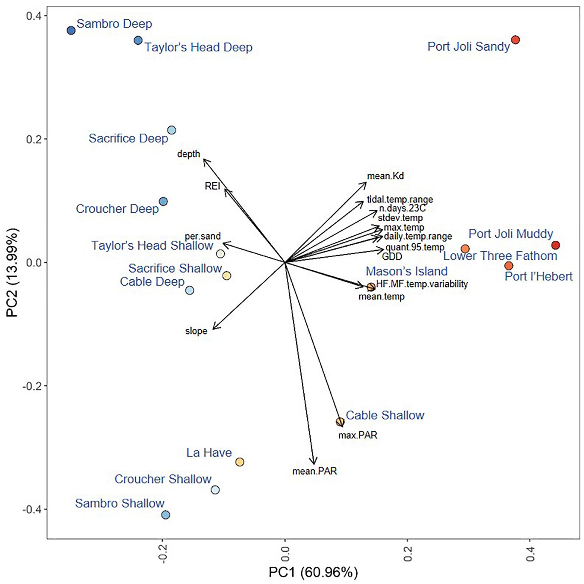
Figure 2. Principal components analysis of environmental metrics measured at each site with currents excluded. Points are colored from red to blue according to their position along the first principal component. Loadings of environmental variables are shown by end points of the black arrows Variable abbreviations are defined in Table 1.

We used lasso regression (least absolute shrinkage and selection operator, Tibshirani, 1996), for model selection and identifying the most important predictor variables for seagrass production and resilience. Lasso regression adds a regularization, or penalty term to regular least-squares multiple regression. This allows for the effective fitting of regression models wherein the number of predictors is near or even larger than the number of observations. The penalty term is on the size (absolute value) of the regression coefficients and this allows for less important or irrelevant regression coefficients to be forced to zero, and omitted from the model (hence the designation of lasso as a shrinkage estimator). The weight given to the regularization term, and hence the variable selection, is controlled by the parameter λ. The lasso regression was implemented with elastic-net regression in the glmnet package in R (Friedman et al., 2010), which estimates λ using k-fold cross-validation. Due to the Monte Carlo variation in the cross-validation procedures (the random splitting of the data into training and validation sets), the lasso procedure was run for 200 randomly assigned training and validation data splits for each biological response metric using the cv.glmnet function in the glmnet package in R (Friedman et al., 2010). For each response metric the final selected set of predictors were those retained when they occurred in all cases.

The selected predictors were then used in subsequent multiple regression models to evaluate the relative influence of each metric on each biological response variable. Because collinearity was present, and an inherent feature of the system, we used a suite of regression fit and diagnostic metrics to evaluate the relative importance of each predictor (Kraha et al., 2012; Nimon and Oswald, 2013; Ray-Mukherjee et al., 2014). In addition to coefficient estimates and Beta weights, squared structure coefficients (r_s²) were used to give information on the proportion of the variance in the regression effect explained by each predictor alone, allowing for a ranking of independent variables based on their contribution to the regression effect (Kraha et al., 2012; Ray-Mukherjee et al., 2014). We also conducted commonality analyses, which decomposes the proportion of variance explained by a regression R² into unique and common effects. Unique effects indicate how much variance is uniquely accounted for by each predictor, and is the incremental difference in the proportion of the variance assigned to a predictor with and without that predictor present in the multiple regression (Ray-Mukherjee et al., 2014). Common effects indicate how much variance is common to a set of predictors, and is the total R² discounted by the unique effects (Ray-Mukherjee et al., 2014). The unique and common effects can be summed to generate an estimate of the total explanatory power of a predictor (r²). We also used dominance analysis (Gen Dom) to identify if a predictor contributed more unique variance than others on average across all models of all-possible-subset sizes (Kraha et al., 2012; Nimon and Oswald, 2013). Finally, we used relative importance weights (RIW) to evaluate the proportional contribution of each predictor to the model’s R² after correcting for the effects of correlations with other predictors (Kraha et al., 2012). Regression metrics were calculated using the yhat package in R (Nimon et al., 2020).

Predictors were then ranked in each model according to r_s², r², GenDom, and RIW. This subset of the regression metrics was chosen to avoid redundant metrics. The rankings were then averaged across these metrics to yield an overall importance ranking for each predictor. We then assessed the relative importance of environmental predictors for each biological response using: (1) the identity of the variables selected by the lasso approach, and (2) the overall ranking of each selected variable, generated by averaging the rankings for the above noted regression fit metrics (Tables 1, 2). To assess the overall importance of each environmental predictor for all biological metrics, the ranking of each environmental metric was then averaged across all the biological models for which it was selected, and then for all models of production and resilience separately. Variable abbreviations are listed in Table 1.

TABLE 1

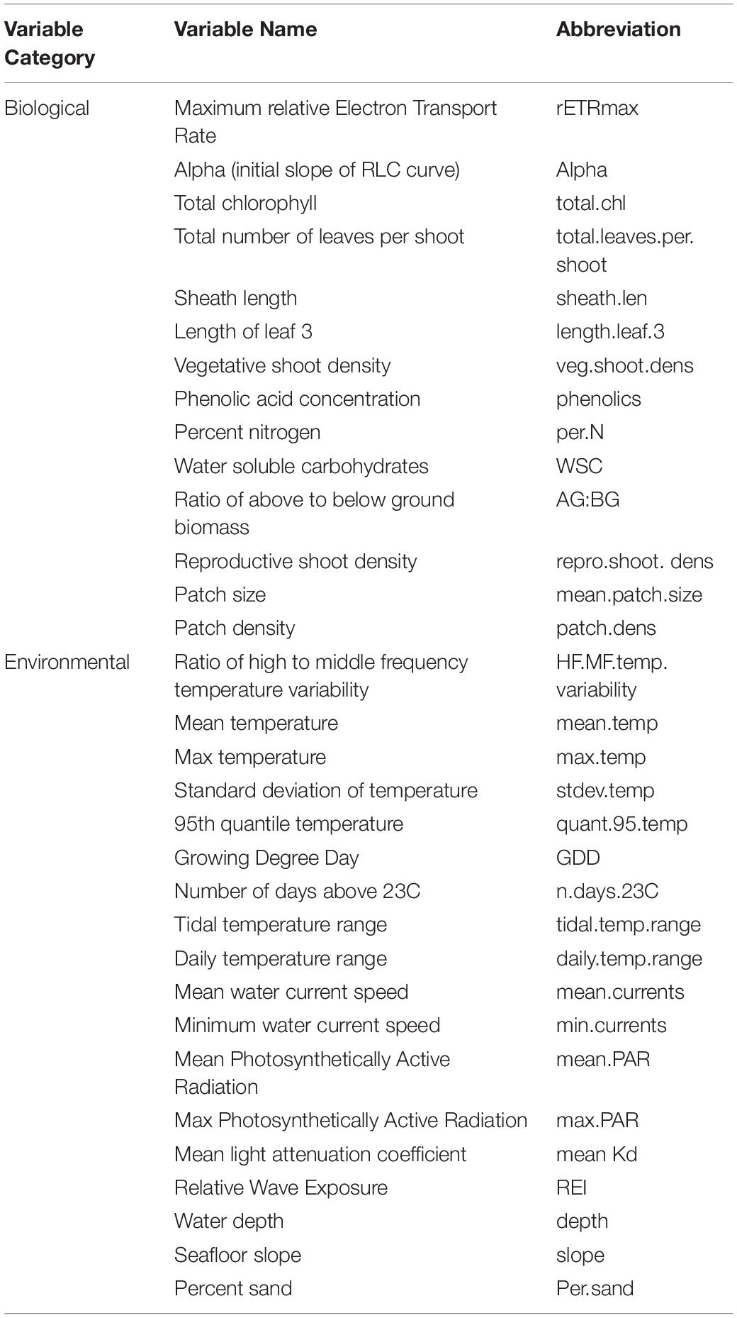
Table 1. Biological and environmental variables, and their abbreviations used throughout the text and figures.

TABLE 2

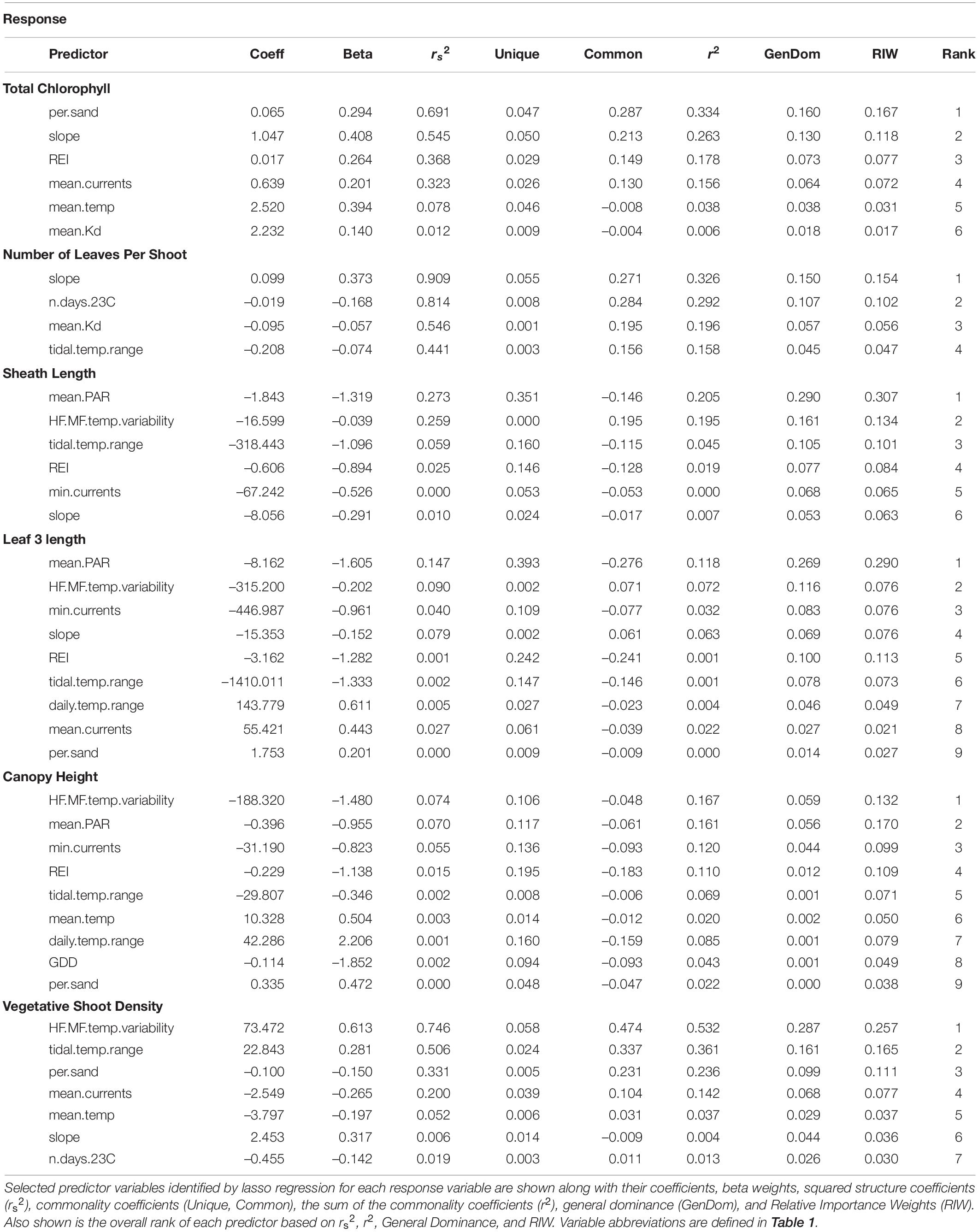
Table 2. Regression results for biological metrics of production.

Results

Environmental Conditions in Eelgrass Beds

The first principal component in the PCA of environmental variables (excluding water currents) explained 61% of the variance across sites (Figure 2). Metrics of temperature (HF:MF variability, mean, maximum, standard deviation, 95th quantile, GDD, days > 23°C, tidal temperature range, and daily temperature range) and light attenuation (mean K_d) had the highest positive loadings on this axis, while depth, slope, REI and percent sand had the highest negative loadings (Figure 2). When water currents were included (by excluding sites without current measurements), PC1 explained 68.2% of the variance, and water currents loaded along the first principal component along with temperature, light, REI, depth, slope, and percent sand (Supplementary Figure S1). The second principal component in the PCAs explained 13.99% without currents and 10% with currents, with only PAR (mean, maximum) strongly loading in both analyses (Figure 2 and Supplementary Figure S1). Sites loaded similarly along the first principal component in both analyses, but warmer sites spread further along the second principal component when currents were included (Figure 2 and Supplementary Figure S1).

Mean temperatures ranged from 8.31 to 10.84°C across all sites. The warmest sites were Port l’Hebert, Port Joli, and Lower Three Fathom (Supplementary Table S2), as these sites generally had the highest extreme temperatures (max and 95th quantile), more days above 23°C, and greater temperature variability (standard deviation of temperature, daily and tidal temperature ranges, HF:MF temperature variability) (Figures 2, 3 and Supplementary Table S2). These warmer sites were also among the shallowest (mean depth at high tide = 0.9–1.7 m) with the highest light attenuation (mean K_d = 0.8–1.62 m^–1), and some of the lowest slope angles (0.14–1.82°), current speeds (mean current speed = 0.66–3.67 cm s^–1), and wave exposure (REI = 3.00–16.39) (Figure 2 and Supplementary Table S1). The warmer, shallower sites also generally had low percent sand (i.e., high percent silt: 27.09–79.26%) in sediments (Supplementary Table S1). The coldest sites were the deep locations at Sambro, Taylor’s Head, Sacrifice, Croucher, and Cable, where mean temperatures and variability were low and temperatures did not exceed 23°C (Figure 2 and Supplementary Table S2). These cooler deep locations (mean depth at high tide = 3.4–6.2 m) had lower light attenuation (mean K_d = 0.39–0.70 m^–1) and PAR (189.74–279.15 μmol m^–2 s^–1), and higher slope angles (1.49–10.77°) (Supplementary Table S1), wave exposure (REI = 19.52–285.82), and current speeds (mean current speed = 3.69–6.61 cm s^–1) than the warmest sites and locations. There were some shallow sites that had moderate mean and maximum temperatures, and low light attenuation, but had high temperature variability, and relatively low current speeds, wave exposures, and slope angles (Mason’s Island, Cable Shallow) (Figure 2 and Supplementary Tables S1, S2). Mean PAR was not strongly correlated with light attenuation, but was negatively correlated with depth, water currents, and wave exposure, and positively correlated with temperature, although these correlations were fairly weak (Figure 3).

FIGURE 3

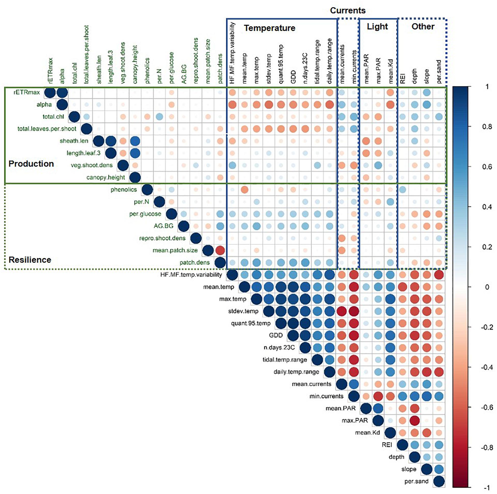
Figure 3. Matrix of Pearson’s correlation coefficients between all environmental and biological metrics. Points are colored and sized according to the value of the Pearson’s correlation coefficient. Biological metrics are shown in green and split into those associated with production and resilience. Environmental metrics are in black and categorized as indicated. Variable abbreviations are defined in Table 1. Plot created using the corrplot package in R (Wei and Simko, 2017).

Biological Metrics Along Environmental Gradients

Biological metrics of production and resilience were examined in terms of their relationships to environmental gradients (Figures 2–5), as well as the relative importance of individual environmental variables for each biological metric (Table 2 for production, Table 3 for resilience). We then looked at the overall importance of environmental metrics across all biological variables (Figure 6).

FIGURE 4

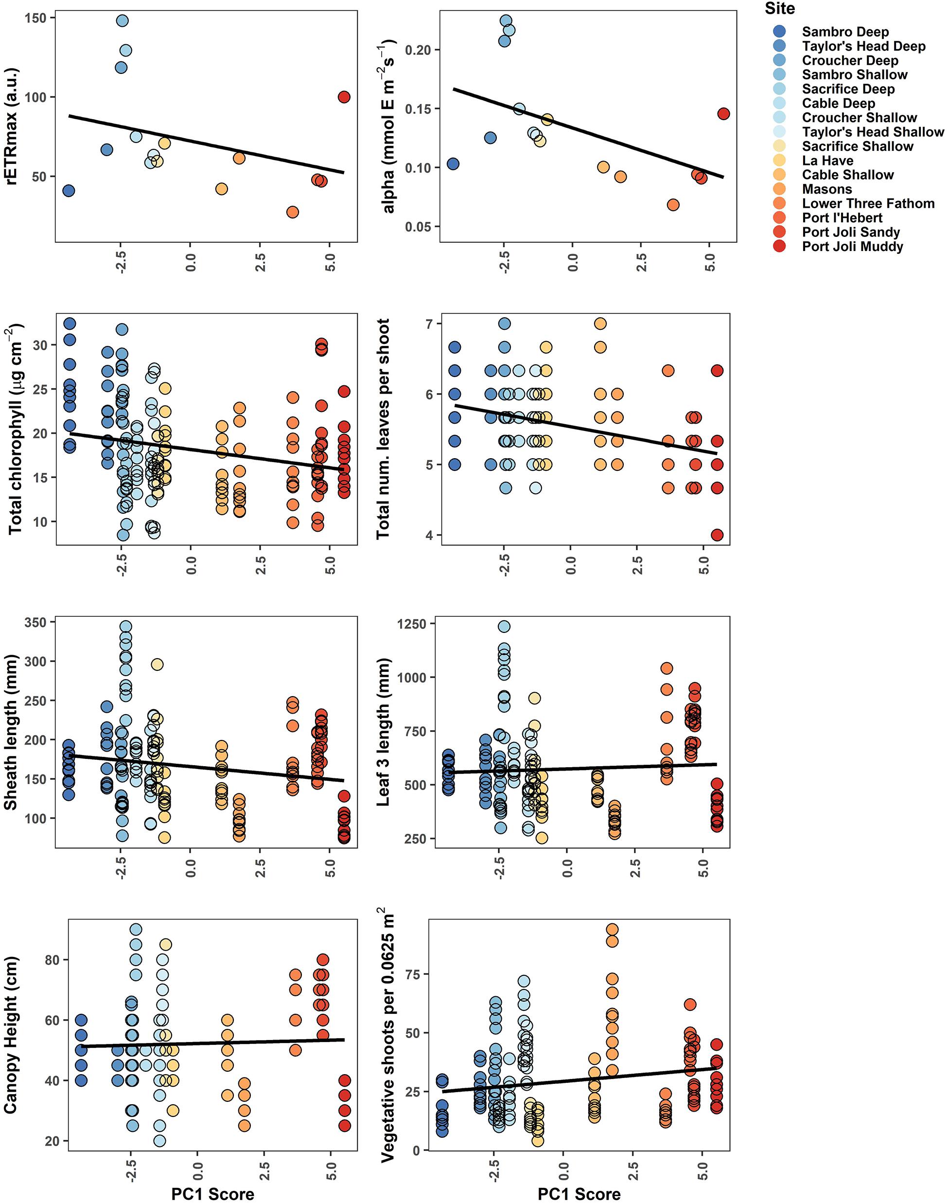
Figure 4. Biological metrics of production plotted against each site’s score along the first principal component in the PCA of environmental variables. The least-squares fit straight line is given in black. Point color corresponds to Figure 2, demonstrating a gradient from cooler, deeper sites (blue) to warmer, shallower sites with higher light attenuation (red).

FIGURE 5

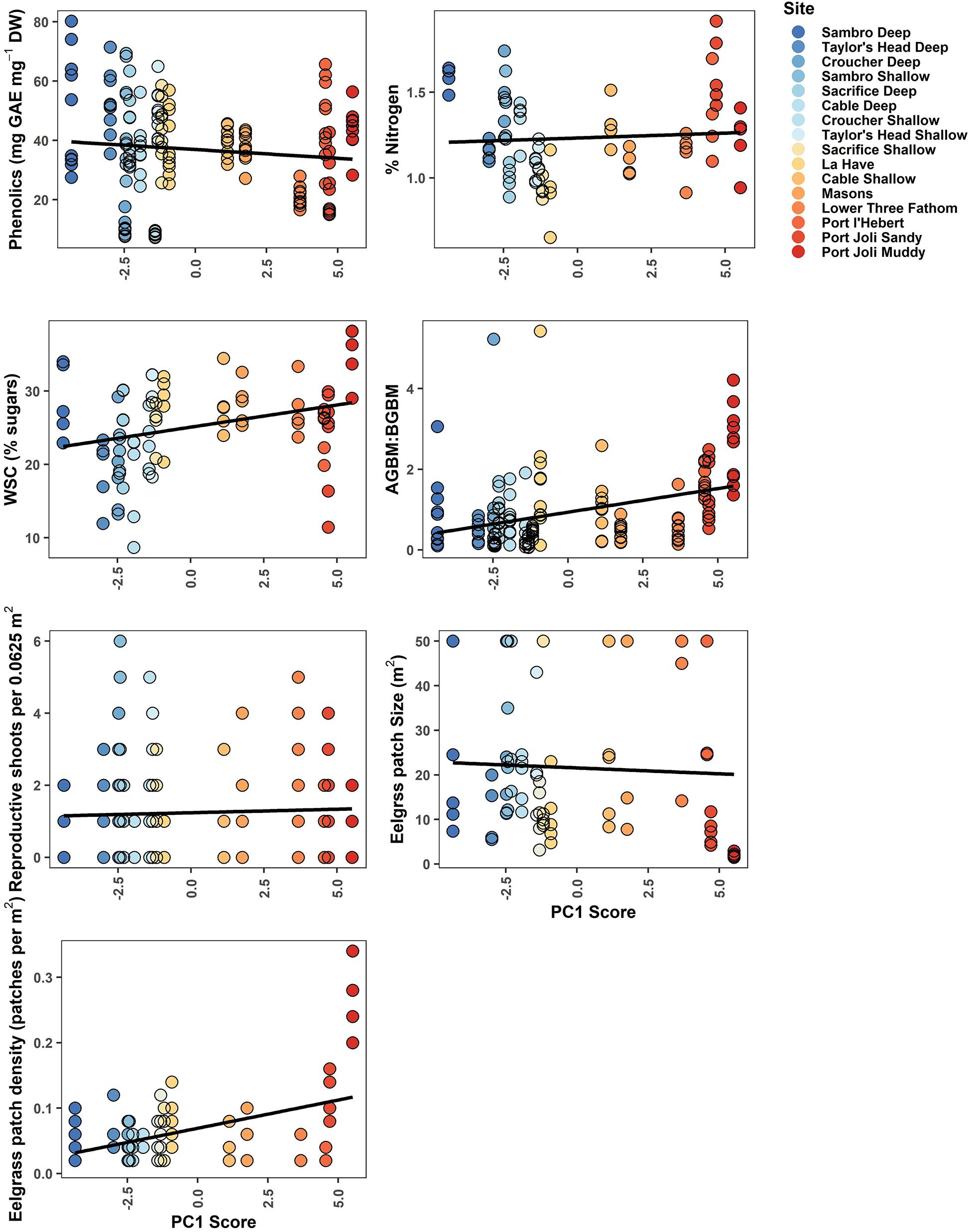
Figure 5. Biological metrics of resilience plotted against each site’s score along the first principal component in the PCA of environmental variables. WSCs were measured in rhizomes, while % Nitrogen was measured in leaves. The least-squares fit straight line is given in black. Point color corresponds to Figure 2, demonstrating a gradient from cooler, deeper sites (blue) to warmer, shallower sites with higher light attenuation (red).

TABLE 3

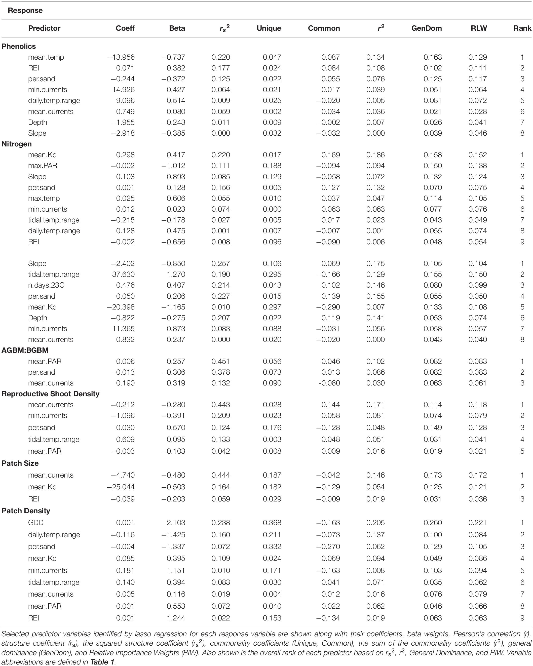
Table 3. Regression results for biological metrics of resilience.

FIGURE 6

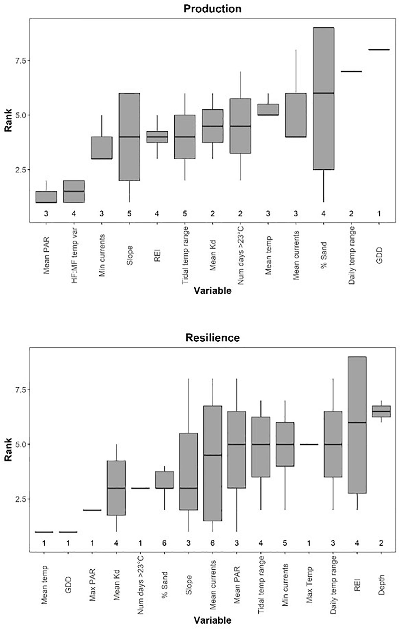
Figure 6. Boxplots of environmental variable ranks in multiple regressions of metrics of production (top panel) and resilience (bottom panel), with lower ranks representing higher importance. Ranks represent averages across squared structure coefficients (r_s²), commonality metrics (r²), general dominance, and Relative Importance Weights. Boxes show the median, first, and third quartiles. Upper and lower whiskers correspond to the largest and smallest values, meeting the condition that they are no further than 1.5 IQR from the first and third quartiles. Numbers for each variable represent the number of models each variable was selected in. Variable abbreviations given in Table 1.

Metrics of Production

Biological metrics of production were plotted against each site’s ranking on the first principal component of the PCA to visualize relationships with the main environmental gradient represented by the sites (temperature, light attenuation, depth, slope, REI, and percent sand) (Figure 4). The photosynthetic parameters rETRmax and alpha tended to decrease along the gradient when moving from deeper cooler sites to shallower warmer sites (rETRmax = 27–148 a.u., α = 0.068–0.225 electrons/photons), except for low values at the two coldest sites (Sambro Deep, Taylor’s Head Deep). Bivariate correlations (Figure 3) were strongest between the two metrics of photosynthetic efficiency (rETRmax and alpha) and temperature variability (HF:MF temperature variability, stdev temp, and the daily temperature range), mean current speeds, mean light attenuation, and slope, with all relationships being negative except with slope and mean current speed. Total chlorophyll (median) also generally decreased along the environmental gradient represented by PC1 (13.4–25.6 μg cm^–2) (Figure 4), and was influenced by positive relationships with percent sand, slope, wave exposure, mean water currents, mean temperature, and mean light attenuation (Figure 3 and Table 2). The median number of leaves per shoot also decreased along the gradient represented by PC1 (5.0–6.0 leaves) (Figure 4), with slope (positive relationship), days above 23°C (negative relationship), mean light attenuation (negative relationship), and the tidal temperature range (negative relationship) as the most important determinants (Figure 3 and Table 2).

Sheath length, leaf length, and canopy height largely showed similar patterns across sites (sheath length = 96.3–296.5 mm, leaf length = 328.8–1022.5 mm, canopy height = 30.0–80.5 cm) (Figure 4). None of these metrics strongly reflected the environmental gradient in PC1, however, they more strongly reflected the gradient in PAR represented by PC2 (Figures 2, 4 and Table 2), being longest at the deeper cooler sites and the warmest, shallowest sites compared to shallow cool sites. HF:MF temperature variability and mean PAR were the top two ranking variables in all three models, with shorter plants at sites with higher short-term temperature variability and higher PAR (Table 2). The next highly ranked variables in these models were the tidal temperature range, minimum current speed, slope, and wave exposure, with the daily temperature range, mean water current speed, mean temperature, GDD, and percent sand also being selected, but ranking lower in importance (Figure 3 and Table 2). Vegetative shoot density did not strongly vary along the environmental gradient represented by PC1 (14.0–57.5 shoots 0.0625 m^–2) (Figure 4), and was most strongly influenced by a positive effect of HF:MF temp variability and tidal temperature range, with the percent sand (negative relationship), mean currents (negative relationship), mean temperature (negative relationship), slope (positive relationship), and the number of days above 23°C (negative relationship) also being selected, but ranking moderately to low in importance (Figure 3 and Table 2).

Metrics of Resilience

Phenolics weakly decreased across the environmental gradient represented by PC1, with the exception of low values at Croucher Shallow and Deep (8.35–52.02 mg GAE mg^–1 DW) (Figure 5). The most important determinants included mean temperature (negative relationship), wave exposure (positive relationship), percent sand (negative relationship), water currents (mean and minimum) (positive relationships), and the daily temperature range (positive relationships), with the other selected variables (slope and depth) being lower in importance (Figure 3 and Table 3). The percent of nitrogen in leaves did change along the environmental gradient represented by PC1 (1.0–1.62%), and was highest at the warmer, shallower sites and the deepest, coolest sites (Figure 5). Values were consistently below the threshold for nitrogen enrichment (1.8% dry weight) (Short, 1987; Duarte, 1990). Percent nitrogen was influenced by mean light attenuation (positive relationship), max PAR (negative relationship), slope (positive relationship), percent sand (positive relationship), maximum temperature (positive relationship), and minimum currents (positive relationship), with the daily and tidal temperature ranges and wave exposure being selected, but ranking lower in importance (Figure 3 and Table 3). WSC in plant rhizomes generally increased along the environmental gradient represented by PC1, ranging from 18.18 to 36.33% dry weight (Figure 5). The environmental metrics driving variation in WSC were slope (negative relationship), tidal temperature range (positive relationship), the number of days above 23°C (positive relationship), percent sand (positive relationship), mean light attenuation (negative relationship), depth (negative relationship), and currents (mean and minimum, positively correlated) (Figure 3 and Table 3).

The ratio of above to belowground biomass increased along the environmental gradient represented by PC1 (0.17–2.73), with higher values at the warmer, shallower sites as compared to the deeper, cooler sites (Figure 5). The most important environmental metrics driving variation were the mean PAR (positive relationship), percent sand (negative relationship), and mean water current speed (positive relationship) (Figure 3 and Table 3). Reproductive shoot densities showed no trend along PC1 (0.1–2.8 shoots 0.0625 m^–2) (Figure 5), being influenced mainly by water current speed (minimum and mean, negative relationships), percent sand (positive relationship), the tidal temperature range (positive relationship), and mean PAR (negative relationship) (Figure 3 and Table 3). Eelgrass patch size showed no trend along PC1 (1.9–50.0 m²) (Figure 5), and was most strongly influenced by negative relationships with mean water current speed, mean light attenuation, and wave exposure (Figure 3 and Table 3). Patch density increased along the environmental gradient represented by PC1 (0.02–0.28 patches m^–2), primarily driven by high patchiness at Port Joli muddy and sandy. Here high patchiness was mainly due to high GDD, low percent sand, and high light attenuation, with minimum and mean water current speed (positive relationship), the tidal temperature range (positive relationship), mean PAR (positive relationship), and wave exposure (positive relationship) being selected in the model, but ranking moderate to low in importance (Figure 3 and Table 3). Daily temperature range also ranked highly in this model, but is likely a suppressor variable, defined as a variable with weak predictive power on its own, but which modifies the predictive power of the other predictors in the model (Kraha et al., 2012). This was evidenced in a mismatch in sign between Beta and r, and a negative Common coefficient (Table 3) (Ray-Mukherjee et al., 2014).

Relative Importance of Environmental Metrics

Metrics of Production

Mean PAR was the most important variable influencing metrics of production, having the highest overall ranking (closest to 1) when averaged across models where it was included as a predictor variable, but it was only selected in three models of seven (Figure 6 and Table 2). HF:MF temperature variability was the second highest ranked metric, occurring in four of the seven models (Figure 6 and Table 2). Mean light attenuation was also among the most important predictors in two models, but ranked lower than six other metrics (Figure 6 and Table 2). Five other metrics of temperature were included in models of production, including the tidal temperature range (ranked 6th, occurring in five models), the number of days above 23°C (ranked 8th, occurring in two models), the mean temperature (ranked 9th, occurring in three models), daily temperature range (ranked 12th, occurring in two models), and GDD (ranked 13th, occurring in one model) (Figure 6 and Table 2).

Metrics of water motion, including current speed (minimum and mean), slope, and wave exposure (REI) were commonly selected in models for production metrics and were relatively highly ranked (3rd, 10th, 4th, and 5th, respectively) (Figure 6 and Table 2). Percent sand (also correlated with REI and water currents) was selected in four of the seven total models, but ranked low in importance (Figure 6 and Table 2). Depth was not selected in any models of production metrics, but is correlated with wave exposure, light, and water currents, and to some degree, percent sand and slope (Figures 3, 6 and Table 2).

Metrics of Resilience

There was higher variability in the importance of environmental variables for resilience metrics than for production, with five variables appearing in only one of the seven models, indicating no single metric influences all aspects of resilience (Figure 6). Other temperature metrics included in the models were mean temperature, GDD, the number of days above 23°C, and max temperature, which were selected in only one model each, but generally had high relative importance (Figure 6 and Table 3). Tidal temperature range and the daily temperature range were selected in three and four models respectively, but generally ranked lower in importance (Figure 6 and Table 3). Mean light attenuation and maximum PAR were the third and fourth highest ranking environmental metrics, with light attenuation appearing in four of the seven models, where it was highly ranked (Figure 6 and Table 3). The percent sand and slope (highly correlated) were moderately ranked relative to other environmental variables for metrics of resilience, appearing in six and three of the seven models, respectively (Figure 6 and Table 3). Metrics of water motion, including wave exposure and currents (minimum and maximum) were also commonly selected in models, but had a low relative importance (Figure 6 and Table 3). Depth was selected in two models, but was less important than other environmental metrics (Figure 6 and Table 3).

Discussion

Our results demonstrate the strong interacting roles of temperature, light, water movement, and sediment characteristics in shaping metrics of eelgrass (Zostera marina) productivity and resilience across a broad range of biological scales (physiological, morphological, population, landscape). Eelgrass sites in this study spanned environmental gradients defined by variation in temperature and light conditions, water movement, depth, and sediment characteristics. Sites with higher mean temperatures also had higher temperature extremes and greater short-term temperature variation (tidal and daily time scales), and were shallower, less exposed to waves and water currents, and had high light attenuation. Zostera marina beds at the warmest sites in our study showed signs of temperature and light stress, which led to apparent declines in photosynthetic efficiency and resilience. This was in contrast to plants at deeper, cooler sites, which were able to maintain high productivity and resilience under low light conditions.

Acclimation to low light in Z. marina was evident at warmer sites through the growth of longer sheaths, leaves, and canopy heights relative to sites with higher light levels, which are morphological changes that increase photosynthetic area (Ruiz and Romero, 2003; Lee et al., 2007; Ochieng et al., 2010; McMahon et al., 2013; Wong et al., 2020a). Plants can also increase tissue pigment concentrations in low light to increase the efficiency of light capture (Ruiz and Romero, 2003; McMahon et al., 2013), but this response was not evident at the warmest sites. Low chlorophyll at warm sites was associated with low rETRmax and alpha, indicating a decline in photosynthetic efficiency in these plants despite more photosynthetic area, which may be linked to heat-induced damage to photosynthetic apparatus (Marin-Guirao et al., 2016).

There were also indications that plants at warmer sites had reduced resilience relative to cooler sites, as phenolic concentrations were lower, the ratio of above to belowground biomass was higher, and beds were patchier. Low phenolic concentrations can arise under low light conditions due to reduced requirements for UV protection or from plants redirecting energy toward more fundamental metabolic processes (Vergeer et al., 1995; Wong et al., 2020a), and represent a reduced defense capacity of plants (Agostini et al., 1998). Losses of belowground biomass occur as carbohydrate reserves are utilized or their production reduced during periods of low photosynthesis to maintain a positive carbon balance (Wong et al., 2020b), and as plants allocate less energy to belowground tissues to reduce the respiratory burden (Fraser et al., 2014; George et al., 2018, Strydom et al., 2020), leading to increases in the ratio of above to belowground biomass in stressed beds. The consequence of this are that plants have smaller energy reserves for times of stress and are more likely to become uprooted. Patchier beds have a lower capacity to recover from additional physical disturbance through asexual vegetative growth from rhizome elongation (Fonseca and Bell, 1998; Rasheed, 2004), and therefore bed continuity is considered a key attribute of resilience to future disturbances (Unsworth et al., 2015).

Reproductive shoot densities were also higher at warmer sites with lower water motion, consistent with a response to stressful conditions intended to better enable population recovery following loss (Díaz-Almela et al., 2007; Cabaco and Santos, 2012). Contrary to our expectations, WSC concentrations were highest at the warmest sites. In fact, heat stressed plants can have high sugar concentrations, which serve a protective function for proteins, membranes, and the photosynthetic apparatus, and therefore sugar metabolism can be downregulated in heat stressed plants (Kaplan and Guy, 2004; Gu et al., 2012; Moreno-Marin et al., 2018). Taken together, these results suggest that plants at the warmest sites in our study are stressed due to a combination of high temperatures, high light attenuation, and low water flow, leading to declines in photosynthetic efficiency and overall resilience relative to cooler sites.

Interestingly, we saw the fewest and shortest leaves at the warmest site in our data set (Port Joli Muddy), likely reflecting conditions that are persistently stressful over the time scale of months to years, leading to a loss of biomass to reduce respiratory demand (Ochieng et al., 2010; McMahon et al., 2013). This site also had the lowest chlorophyll concentration, which, combined with a reduction in tissue mass suggests a decline in plant ability to acclimate to low light conditions (Ochieng et al., 2010). Plants at this site also had the highest concentration of WSC and ratio of above to below ground biomass, the lowest reproductive shoot densities, and the patchiest bed, providing clear indications of low productivity and resilience at the extreme end of the environmental gradient present in our study.

Acclimation to low light conditions was also evident at the coldest sites in our study through morphological changes that increase light capture (e.g., increases in the length and number of leaves), similar to what was observed under low light conditions at the warmest sites. However, in contrast to the warm sites, eelgrass at the coldest and deepest sites in our study had relatively high tissue pigment concentrations and photosynthetic efficiency (Ruiz and Romero, 2003; Lee et al., 2007; Ochieng et al., 2010; McMahon et al., 2013; Wong et al., 2020a). The cooler temperatures at these sites likely play a role in increasing the ability of seagrasses to tolerate low light conditions through decreases in respiratory demand (Lee et al., 2007). In addition, high water movement may have contributed to higher photosynthetic efficiency by thinning the diffusive boundary layer and increasing photosynthetic carbon uptake (Jones et al., 2000; Koch, 2001). Plants at cooler, deeper sites also had higher concentrations of phenolics, low above to belowground biomass ratios, and less patchy beds. Taken together, these results suggest that cooler temperatures and higher water movement are conducive to the maintenance of high productivity despite low light conditions, and allow Z. marina to maintain high resilience relative to warmer, shallower sites.

Vegetative shoot densities are linked to the overall capacity of an eelgrass bed for growth and expansion, and low shoot densities can indicate stress or disturbance (Lopez y Royo et al., 2010; Ochieng et al., 2010; McMahon et al., 2013). We did not observe a clear relationship between the environmental gradients in this study and shoot densities, and there was no indication that sites where plants displayed other indicators of stress and reduced resilience had lower shoot densities. In fact, shoot densities in some cases were higher where temperature was warmer and light was lower, possibly reflecting a photo-acclimation response to high stress by increasing photosynthetic area, although this was not a consistent pattern. Previous work has shown that seagrass structural metrics, such as shoot density, are slower to respond to environmental stressors. While shoot densities are good general indicators of long-term stress, physiological, biochemical, growth, and morphological metrics are typically more useful for detecting short-term changes in environmental conditions and for identifying specific stressors (Oliva et al., 2012; Roca et al., 2016). Consistent with our results, this points to the importance of monitoring a variety of biological metrics to capture a range of possible responses to environmental change over varying time scales (Romero et al., 2007; Roca et al., 2016). Our results suggest that photosynthetic efficiency, number of leaves, WSC, the ratio of above to below ground biomass, and eelgrass continuity were the biological metrics most responsive in our system to environmental conditions, and may be the most useful for future monitoring.

Our analysis also shows that temperature and light play important roles in influencing eelgrass production and resilience (e.g., Lee et al., 2007; Marbà and Duarte, 2010; Lefcheck et al., 2017; Strydom et al., 2020). Temperature and light metrics were selected in nearly all models, and generally ranked high in importance relative to other environmental variables. However, there was no single temperature metric that was important for all, or even the majority of biological responses. Mean temperature, GDD, the maximum temperature, and the number of days above 23°C were each important determinants of biological responses, but were selected in few models each. Metrics relating to the magnitude of short-term temperature variability (the ratio of high to mid frequency temperature variability and the tidal and daily temperature ranges) were the most commonly selected temperature metrics, and they generally ranked high in importance. Spikes in temperature associated with solar heating during low tides are characteristic of shallow intertidal communities (Wong et al., 2013; Collier and Waycott, 2014; George et al., 2018), and short-term exposure to high temperatures has been linked to declines in seagrass biomass and performance (Biebl and McRoy, 1971; Marsh et al., 1986; Moore et al., 2014; George et al., 2018; Shields et al., 2019). Most previous studies have characterized the effects of high temperature exposure events associated with heat waves or extreme low tides, rather than the effects of repeated thermal stress during regular daily or tidal cycles throughout the growing season (but see Stapel et al., 1997; Moore et al., 2014; Pedersen et al., 2016; George et al., 2018). Our results suggest that gradients of productivity, and to some degree resilience, were related to the extent to which eelgrass beds experience large changes in temperature over short time periods, and indicate that the effects of repeated exposures to high and low temperature conditions should be more widely considered at a mechanism of stress in eelgrass plants (Zimmerman, 2006; Lefcheck et al., 2017).

Water motion (water currents, wave exposure, and seafloor slope) and sediment characteristics have been linked to spatial patterns in eelgrass landscapes through relationships with temperature, seawater and sediment chemistry, and rates of physical disturbance (Goodman et al., 1995; Fonseca and Bell, 1998; Koch, 2001; Pérez et al., 2007; Krause-Jensen et al., 2011), and were commonly selected in models of eelgrass productivity and resilience in our analysis. Low water current speed, slope, exposure, and percent sand in sediments were associated with reduced eelgrass productivity and resilience, but these environmental metrics were less important overall than temperature and light. Temperature and light are influenced by depth and water movement, and our analysis shows that biological responses are likely not driven primarily by any explicit effects of depth and water movement, but rather by the effects of temperature and light directly.

In order to identify the most important environmental predictor variables that explained the biological production and resilience metrics, we made use of lasso regression for variable selection. The selected variables were chosen on the basis of a regularization weight which in each case was identified by cross-validation and optimizing the predictive skill of the regression model. We elected to use a suite of regression fit metrics in our multiple regressions modeling to interpret the relative importance of predictor variables. This was largely due to the multicollinearity that arose from the correlation of the predictor variables, which was an inherent feature of the system. A more typical approach is to remove collinear variables before modeling, but this requires an a priori value judgment as to which variable is more important. Our use of a suite of fit metrics allows for interpretations of how collinear variables work together, and which variables play the strongest role in influencing variance independently, as well as in concert with other variables (Kraha et al., 2012). For instance, all metrics of temperature used in our analysis were highly collinear, and were strongly correlated with other environmental variables in our data set, but evaluating their relative importance with a suite of fit metrics enabled a robust assessment of how different aspects of temperature (mean, extremes, ranges, variability at different frequencies) influence seagrass emergent properties. This allowed a more nuanced interpretation of temperature effects on eelgrass.

Conclusion

Our research is among the first to use suites of biological metrics along environmental gradients to identify conditions conducive to high eelgrass productivity and resilience. We identify temperature and light as the primary factors that drive variation in ecosystem status across a spatial gradient of ∼225 km, linking warm water, high temperature variability over daily and tidal cycles, high light attenuation and low water movement to reduced productivity and resilience. Our results demonstrate that one single environmental metric does not explain variation in all biological properties across sites. In particular, bioindicators showed unique responses to different characterizations of temperature (e.g., mean, maximum, high frequency temperature variability) pointing to a wide range of temperature effects on eelgrass ecosystems. For example, we show that short duration thermal stress repeated on tidal and daily cycles has important negative consequences for eelgrass productivity and resilience. These results highlight the complex role of environmental factors in shaping coastal ecosystems, and indicate that a complete understanding of the effects of global climate change requires a more nuanced approach that not only characterizes changes to the mean, but also to the extremes and variability over different time scales. Moreover, analyses that allow for collinearity enable a more detailed investigation of how different characterizations of environmental change shape ecosystem responses, and can elucidate the multiple ways in which global climate change is impacting the processes that support the function and resilience of coastal ecosystems.

Data Availability Statement

The raw data supporting the conclusions of this article will be made available by the authors, without undue reservation.

Author Contributions

KK created the sampling design, collected the data, designed and performed the analysis, and led the manuscript writing. MD designed the analysis and contributed to the manuscript text. MW conceived of the study, created the sampling design, collected the data, designed the analysis, and contributed to the manuscript text. All the authors contributed to the article and approved the submitted version.

Funding

This research was funded by Fisheries and Oceans Canada (MW) and an NSERC Discovery Grant (MD).

Conflict of Interest

The authors declare that the research was conducted in the absence of any commercial or financial relationships that could be construed as a potential conflict of interest.

Acknowledgments

We thank M. Bravo, S. Roach, G. Griffiths, A. MacDonald, B. Vercaemer, M. Wilson, S. Armsworthy, and D. Hardy for field support, and M Bravo, B. Vercaemer, T. Perry, A. Campbell, D. Krug, C. Siong, J. Hogenbom, B. Roethlisberger, M. Scarrow, and G. Griffiths for assistance in the laboratory.

Supplementary Material

The Supplementary Material for this article can be found online at: https://www.frontiersin.org/articles/10.3389/fmars.2021.597707/full#supplementary-material

References

Agostini, S., Desjobert, J.-M., and Pergent, G. (1998). Distribution of phenolic compounds in the seagrass Posidonia oceanica. Phytochemisty 48, 611–617. doi: 10.1016/s0031-9422(97)01118-7

CrossRef Full Text | Google Scholar

Bakirman, T., and Gumusay, M. U. (2020). A novel GIS-MCDA-based spatial habitat suitability model for Posidonia oceanica in the Mediterranean. Environ. Monitor. Assess. 192, 1–13. doi: 10.4018/978-1-7998-5027-4.ch001

CrossRef Full Text | Google Scholar

Barbier, E. B., Hacker, S. D., Kennedy, C., Koch, E. W., Stier, A. C., and Silliman, B. R. (2011). The value of estuarine and coastal ecosystem services. Ecol. Monogr. 81, 169–193.

Google Scholar

Bertelli, C. M., Creed, J. C., Nuuttila, H. K., and Unsworth, R. K. F. (2020). The response of the seagrass Halodule wrightii ascherson to environmental stressors. Estuar. Coast. Shelf. Sci. 238:106693. doi: 10.1016/j.ecss.2020.106693

CrossRef Full Text | Google Scholar

Biebl, R., and McRoy, C. P. (1971). Plasmatic resistance and rate of respiration and photosynthesis of Zostera marina at different salinities and temperatures. Mar. Biol. 8, 48–56. doi: 10.1007/bf00349344

CrossRef Full Text | Google Scholar

Bostrom, C., Roos, C., and Ronnberg, O. (2004). Shoot morphometry and production dynamics of eelgrass in the northern Baltic Sea. Aquat. Bot. 79, 145–161. doi: 10.1016/j.aquabot.2004.02.002

CrossRef Full Text | Google Scholar

Cabaco, S., and Santos, R. (2012). Seagrass reproductive effort as an ecological indicator of disturbance. Ecol. Indic. 23, 116–122. doi: 10.1016/j.ecolind.2012.03.022

CrossRef Full Text | Google Scholar

Cabello-Pasini, A., Muniz-Salazar, R., and Ward, D. H. (2003). Annual variations of biomass and photosynthesis in Zostera marina at its southern end of distribution in the North Pacific. Aquat. Bot. 76, 31–47. doi: 10.1016/s0304-3770(03)00012-3

CrossRef Full Text | Google Scholar

Campbell, S. J., McKenzie, L. J., and Kerville, S. P. (2006). Photosynthetic responses of seven tropical seagrass to elevated seawater temperature. J. Exp. Mar. Biol. Ecol. 330, 455–468. doi: 10.1016/j.jembe.2005.09.017

CrossRef Full Text | Google Scholar

Chan, K. S., and Ripley, B. (2012). TSA: Time Series Analysis. R Package Version 1.01.

Google Scholar

Collier, C. J., and Waycott, M. (2014). Temperature extremes reduce seagrass growth and induce mortality. Mar. Poll. Bull. 83, 483–490. doi: 10.1016/j.marpolbul.2014.03.050

PubMed Abstract | CrossRef Full Text | Google Scholar

Díaz-Almela, E., Marbà, N., and Duartem, C. M. (2007). Fingerprints of Mediterranean sea warming in seagrass (Posidonia oceanica) flowering records. Glob. Change Biol. 13, 224–235. doi: 10.1111/j.1365-2486.2006.01260.x

CrossRef Full Text | Google Scholar

Duarte, C. M. (1990). Seagrass nutrient content. Mar. Ecol. Prog. Ser. 67, 201–207.

Google Scholar

DuBois, K., Abbott, J. M., Williams, S. L., and Stachowicz, J. J. (2019). Relative performance of eelgrass genotypes shifts during an extreme warming event, disentangling the roles of multiple traits. Mar. Ecol. Prog. Ser. 615, 67–77. doi: 10.3354/meps12914

CrossRef Full Text | Google Scholar

Ebell, L. F. (1969). Specific total starch determinations in conifer tissues with glucose oxidase. Phytochemisty 8, 25–36. doi: 10.1016/s0031-9422(00)85790-8

CrossRef Full Text | Google Scholar

Evans, A. S., Webb, K. L., and Penhale, P. A. (1986). Photosynthetic temperature acclimation in two coexisting seagrasses, Zostera marina L. and Ruppia maritima. Aquat. Bot. 24, 185–197. doi: 10.1016/0304-3770(86)90095-1

CrossRef Full Text | Google Scholar

Filbee-Dexter, K., and Wernberg, T. (2018). Rise of turfs: a new battlefront for globally declining kelp forests. BioScience 68, 64–76. doi: 10.1093/biosci/bix147

CrossRef Full Text | Google Scholar

Fonseca, M., Whitfield, P. E., Kelly, N. M., and Bell, S. S. (2002). Modelling seagrass landscape pattern and associated ecological attributes. Ecol. App. 12, 218–237. doi: 10.1890/1051-0761(2002)012[0218:mslpaa]2.0.co;2

CrossRef Full Text | Google Scholar

Fonseca, M. S., and Bell, S. S. (1998). Influence of physical setting on seagrass landscapes near Beaufort, North Carolina, USA. Mar. Ecol. Prog. Ser. 171, 109–121. doi: 10.3354/meps171109

CrossRef Full Text | Google Scholar

Fourqurean, J. W., Duarte, C. M., Kennedy, H., Marba, N., Holmer, M., Mateo, M. A., et al. (2012). Seagrass ecosystems as a globally significant carbon stock. Nat. Geosci. 5, 505–509. doi: 10.1038/ngeo1477

CrossRef Full Text | Google Scholar

Fraser, M. W., Kendrick, G. A., Statton, J., Hovey, R. K., Zavala-Perez, A., and Walker, D. I. (2014). Extreme climate events lower resilience of foundation seagrass at edge of biogeographical range. J. Ecol. 102, 1528–1536. doi: 10.1111/1365-2745.12300

CrossRef Full Text | Google Scholar

Friedman, J., Hastie, T., and Tibshirani, R. (2010). Regularization Paths for generalized linear models via coordinate descent. J. Stat. Soft. 33, 1–22.

Google Scholar

Gao, Y., Fang, J., Du, M., Fang, J., Jiang, W., and Jiang, Z. (2017). Response of the eelgrass (Zostera marina L.) to the combined effects of high temperatures and the herbicide, atrazine. Aquat. Bot. 142, 41–47. doi: 10.1016/j.aquabot.2017.06.005

CrossRef Full Text | Google Scholar

George, R., Gullstrom, M., Mangora, M. M., Mtolera, M. S. P., and Bjork, M. (2018). High midday temperature stress has stronger effects on biomass than on photosynthesis: a mesocosm experiment on four tropical seagrass species. Ecol. Evol. 9, 4508–4514. doi: 10.1002/ece3.3952

PubMed Abstract | CrossRef Full Text | Google Scholar

Goodman, J. L., Moore, K. A., and Dennison, W. C. (1995). Photosynthetic responses of eelgrass (Zostera marina L.) to light and sediment sulfide in a shallow barrier island lagoon. Aquat. Bot. 50, 37–47. doi: 10.1016/0304-3770(94)00444-q

CrossRef Full Text | Google Scholar

Gu, J., Weber, K., Klempt, E., Winters, G., Franssen, S. U., Wienpahl, I., et al. (2012). Identifying core features of adaptive metabolic mechanisms for chronic heat stress attenuation contributing to systems robustness. Integr. Biol. 4, 480–493. doi: 10.1039/c2ib00109h

PubMed Abstract | CrossRef Full Text | Google Scholar

Hammer, K. J., Borum, J., Hasler-Sheetal, H., Shields, E. C., Sand-Jensen, K., and Moore, K. A. (2018). High temperatures cause reduced growth, plant death and metabolic changes in eelgrass Zostera marina. Mar. Ecol. Prog. Ser. 604, 121–132. doi: 10.3354/meps12740

CrossRef Full Text | Google Scholar

Jones, J. I., Eaton, J. W., and Hardwick, K. (2000). The influence of periphyton on boundary layer conditions: pH microelectrode investigation. Aquat. Bot. 67, 191–206. doi: 10.1016/s0304-3770(00)00089-9

CrossRef Full Text | Google Scholar

Kaplan, F., and Guy, C. L. (2004). Beta-amylase induction and the protective role of maltose during temperature shock. Plant. Physiol. 135, 1674–1684. doi: 10.1104/pp.104.040808

PubMed Abstract | CrossRef Full Text | Google Scholar

Keddy, P. A. (1982). Quantifying within-lake gradients of wave energy: interrelationships of wave energy, substrate particle size and shoreline plants in Axe Lake, Ontario. Aquat. Bot. 14, 41–58. doi: 10.1016/0304-3770(82)90085-7

CrossRef Full Text | Google Scholar

Kim, J.-H., Kim, S. H., Kim, Y. K., Park, J.-I., and Lee, K.-S. (2016). Growth dynamics of the seagrass Zostera japonica at its upper and lower distributional limits in the intertidal zone. Estuar. Coast. Shelf. Sci. 175, 1–9. doi: 10.1016/j.ecss.2016.03.023

CrossRef Full Text | Google Scholar

Kirk, J. T. O. (2011). Light and Photosynthesis in Aquatic Ecosystems, 3rd Edn. Cambridge: Cambridge University Press, 151. doi: 10.1017/CBO9781139168212

CrossRef Full Text | Google Scholar

Koch, E. W. (2001). Beyond light: physical, geological, and geochemical parameters as possible submersed aquatic vegetation habitat requirements. Estuaries Coasts 24, 1–17. doi: 10.2307/1352808

CrossRef Full Text | Google Scholar

Kraha, A., Turner, H., Nimon, K., Zientek, L. R., and Henson, R. K. (2012). Tools to support interpreting multiple regression in the face of multicollinearity. Front. Psychol. 3:44. doi: 10.3389/fpsyg.2012.00044

PubMed Abstract | CrossRef Full Text | Google Scholar

Krause-Jensen, D., Carstensen, J., Nielsen, S. L., Dalsgaard, T., Christensen, P. B., Fossing, H., et al. (2011). Sea bottom characteristics effect depth limits of eelgrss Zostera marina. Mar. Ecol. Prog. Ser. 425, 91–102. doi: 10.3354/meps09026

CrossRef Full Text | Google Scholar

Krumhansl, K., Byrnes, J., Okamoto, D., Rassweiler, A., Novak, M., Bolton, J. J., et al. (2016). Global patterns of kelp forest change over the past half-century. Proc. Nat. Acad. Sci. U.S.A. 113, 13785–13790.

Google Scholar

Krumhansl, K., Dowd, M., and Wong, M. C. (2020). A characterization of the physical environment at eelgrass (Zostera marina) sites along the Atlantic coast of Nova Scotia. Can. Tech. Rep. Fish. Aquat. Sci. 3361, 1–213.

Google Scholar

Krumhansl, K. A., and Scheibling, R. E. (2012). Production and fate of kelp detritus. Mar. Ecol. Prog. Ser. 467, 281–302. doi: 10.3354/meps09940

CrossRef Full Text | Google Scholar

Lavery, P. S., Reid, T., Hyndes, G. A., and Van Elven, B. R. (2007). Effect of leaf movement on epiphytic algal biomass of seagrass leaves. Mar. Ecol. Prog. Ser. 338, 97–106. doi: 10.3354/meps338097

CrossRef Full Text | Google Scholar

Lee, K.-S., Park, S. R., and Kim, Y. K. (2005). Production dynamics of the seagrass, Zostera marina in two bay systems on the south coast of the Korean peninsula. Mar. Biol. 147, 1091–1108. doi: 10.1007/s00227-005-0011-8

CrossRef Full Text | Google Scholar

Lee, K.-S., Park, S. R., and Kim, Y. K. (2007). Effects of irradiance, temperature, and nutrients on growth dynamics of seagrasses: a review. J. Exp. Mar. Biol. Ecol. 350, 144–175. doi: 10.1016/j.jembe.2007.06.016

CrossRef Full Text | Google Scholar

Lefcheck, J. S., Wilcox, D. J., Murphy, R. R., Marion, S. R., and Orth, R. J. (2017). Multiple stressors threaten the imperiled coastal foundation species eelgrass (Zostera marina) in Chesapeake Bay, USA. Glob. Change. Biol. 23, 3474–3483. doi: 10.1111/gcb.13623

PubMed Abstract | CrossRef Full Text | Google Scholar

Lopez y Royo, C., Casazza, G., Pergent-Martini, C., and Pergent, G. (2010). A biotic index using the seagrass Posidonia oceanica (BiPo), to evaluate ecological status of coastal waters. Ecol. Ind. 10, 380–389. doi: 10.1016/j.ecolind.2009.07.005

CrossRef Full Text | Google Scholar

Lotze, H. K., Lenihan, H. S., Bourque, B. J., Bradbury, R. H., Cooke, R. G., Kay, M. C., et al. (2006). Depletion, degradation, and recovery potential of estuaries and coastal seas. Science 312, 1806–1809. doi: 10.1126/science.1128035

PubMed Abstract | CrossRef Full Text | Google Scholar

Marbà, N., and Duarte, C. M. (2010). Mediterranean warming triggers seagrass (Posidonia oceanica) shoot mortality. Glob. Change. Biol. 16, 2366–2375. doi: 10.1111/j.1365-2486.2009.02130.x

CrossRef Full Text | Google Scholar

Marin-Guirao, L., Ruiz, J. M., Dattolo, E., Garcia-Munox, R., and Procaccini, G. (2016). Physiological and molecular evidence of differential short-term heat tolerance in Mediterranean seagrasses. Sci. Rep. 6:28615.

Google Scholar

Marsh, J. A., Dennison, W. C., and Alberte, R. S. (1986). Effects of temperature on photosynthesis and respiration in eelgrass (Zostera marina). J. Exp. Mar. Biol. Ecol. 101, 257–267. doi: 10.1016/0022-0981(86)90267-4

CrossRef Full Text | Google Scholar

Martínez-Crego, B., Vergés, A., Alcoverro, T., and Romero, J. (2008). Selection of multiple seagrass indicators for environmental biomonitoring. Mar. Ecol. Prog. Ser. 361, 93–109. doi: 10.3354/meps07358

CrossRef Full Text | Google Scholar

McMahon, K., Collier, C., and Lavery, P. S. (2013). Identifying robust bioindicators of light stress in seagrasses: a meta-analysis. Ecol. Ind. 30, 7–15. doi: 10.1016/j.ecolind.2013.01.030

CrossRef Full Text | Google Scholar

Moore, K. A., Shields, E. C., and Parrish, D. B. (2014). Impacts of varying estuarine temperature and light conditions on zostera marina (Eelgrass) and its Interactions With Ruppia maritima (Widgeongrass). Estuaries Coasts 37, 20–30. doi: 10.1007/s12237-013-9667-3

CrossRef Full Text | Google Scholar

Moreno-Marin, F., Brun, F. G., and Pedersen, M. F. (2018). Additive response to multiple environmental stressors in the seagrass Zostera marina. Limnol. Oceanogr. 63, 1528–1544. doi: 10.1002/lno.10789

CrossRef Full Text | Google Scholar

Murphy, G. E. P., Wong, M. C., and Lotze, H. K. (2019). A human impact metric for coastal ecosystems with application to seagrass beds in Atlantic Canada. FACETS 4, 210–237. doi: 10.1139/facets-2018-0044

CrossRef Full Text | Google Scholar

Neuheimer, A. B., and Taggart, C. T. (2007). The growing degree-day and fish size-at-age: the overlooked metric. Can J Fish Aquat. Sci. 64, 375–385. doi: 10.1139/f07-003

CrossRef Full Text | Google Scholar

Nimon, K., Oswald, F., and Roberts, J. K. (2020). yhat: Interpreting Regression Effects. R package version 2.0-2.

Google Scholar

Nimon, K. F., and Oswald, F. L. (2013). Understanding the results of multiple linear regression beyond standardized regression coefficients. Org. Res. Methods. 16, 650–674. doi: 10.1177/1094428113493929

CrossRef Full Text | Google Scholar

Ochieng, C. A., Short, F. T., and Walker, D. I. (2010). Photosynthetic and morphological responses of eelgrass (Zostera marina L.) to a gradient of light conditions. J. Exp. Mar. Biol. Ecol. 382, 117–124. doi: 10.1016/j.jembe.2009.11.007

CrossRef Full Text | Google Scholar

Odum, E. P., and Barrett, G. W. (1971). Fundamentals of Ecology, Vol. 3. Philadelphia: Saunders.

Google Scholar

Oksanen, J., Blanchet, F. G., Friendly, M., Kindtx, R., Legendre, P., McGlinn, D., et al. (2019). Vegan: Community Ecology Package. R Package Version 2.5-6.

Google Scholar

Oliva, S., Mascaró, O., Llagostera, I., Pérez, M., and Romero, J. (2012). Selection of metrics based on the seagrass Cymodocea nodosa and development of a biotic index (CYMOX) for assessing ecological status of coastal and transitional waters. Estuar. Coast. Shelf Sci. 114, 7–17. doi: 10.1016/j.ecss.2011.08.022

CrossRef Full Text | Google Scholar

Oliver, E. C., Donat, M. G., Burrows, M. T., Moore, P. J., Smale, D. A., Alexander, L. V., et al. (2018). Longer and more frequent marine heatwaves over the past century. Nat. Commun. 9:1324.

Google Scholar

Pedersen, O., Colmer, T. D., Borum, J., Zavala-Perez, A., and Kendrick, G. A. (2016). Heat stress of two tropical seagrass species during low tides–impact on underwater net photosynthesis, dark respiration and dielin situ internal aeration. New Phytol. 210, 1207–1218. doi: 10.1111/nph.1390

CrossRef Full Text | Google Scholar

Pérez, M., Invers, O., Ruiz, J. M., Frederiksen, M. S., and Holmer, M. (2007). Physiological responses of the seagrass Posidoniaoceanica to elevated organic matter content in sediments: an experimental assessment. J. Exp. Mar. Biol. Ecol. 344, 149–160. doi: 10.1016/j.jembe.2006.12.020

CrossRef Full Text | Google Scholar

Platt, T., Gallegos, C. L., and Harrison, W. G. (1980). Photoinhibition of photosynthesis in natural assemblages of marine phytoplankton. J. Mar. Res. 38, 687–701.

Google Scholar

R Core Team, (2017). R: A Language and Environment for Statistical Computing. Vienna: R Foundation for Statistical Computing.

Google Scholar

Ralph, P. J., and Gademann, R. (2005). Rapid light curves: a powerful tool to assess photosynthetic efficiency. Aquat. Bot. 82, 222–237. doi: 10.1016/j.aquabot.2005.02.006

CrossRef Full Text | Google Scholar

Rasheed, M. A. (2004). Recovery and succession in a multi-species tropical seagrass meadow following experimental disturbance: the role of sexual and asexual reproduction. J. Exp. Mar. Biol. Ecol. 310, 13–45. doi: 10.1016/j.jembe.2004.03.022

CrossRef Full Text | Google Scholar

Rasheed, M. A., and Unsworth, R. K. F. (2011). Long-term climate-associated dynamics of a tropical seagrass meadow, implications for the future. Mar. Ecol. Prog. Ser. 422, 93–103. doi: 10.3354/meps08925

CrossRef Full Text | Google Scholar

Ray-Mukherjee, J., Nimon, K., Mukherjee, S., Morris, D. W., Slotow, R., and Hamer, M. (2014). Using commonality analysis in multiple regressions: a tool to decompose regression effects in the face of multicollinearity. Methods Ecol. Evol. 5, 320–328. doi: 10.1111/2041-210x.12166

CrossRef Full Text | Google Scholar

Richardson, J., Lefcheck, J., and Orth, R. (2018). Warming temperatures alter the relative abundance and distribution of two co-occurring foundational seagrasses in Chesapeake Bay, USA. Mar. Ecol. Prog. Ser. 599, 65–74. doi: 10.3354/meps12620

CrossRef Full Text | Google Scholar

Roca, G., Alcoverro, T., Krause-Jensen, D., Balsby, T. J. S., van Katwijk, M. M., Marba, N., et al. (2016). Response of seagrass indicators to shifts in environmental stressors: a global review and management synthesis. Ecol. Ind. 63, 310–323. doi: 10.1016/j.ecolind.2015.12.007

CrossRef Full Text | Google Scholar

Romero, J., Martinez-Crego, B., Alcoverro, T., and Perez, M. (2007). A multivariate index based on the seagrass Posidonia oceanica (POMI) to assess ecological status of coastal waters under the water framework directive (WFD). Mar. Poll. Bull. 55, 196–204. doi: 10.1016/j.marpolbul.2006.08.032

PubMed Abstract | CrossRef Full Text | Google Scholar

Ruiz, J. M., and Romero, J. (2003). Effects of disturbances caused by coastal constructions on spatial structure, growth dynamics and photosynthesis of the seagrass Posidonia oceanica. Mar. Pollut. Bull. 46, 1523–1533. doi: 10.1016/j.marpolbul.2003.08.021

PubMed Abstract | CrossRef Full Text | Google Scholar

Saava, I., Bennett, S., Roca, G., Jorda, G., and Marba, N. (2018). Thermal tolerance of Mediterranean marine macrophytes: vulnerability to global warming. Ecol. Evol. 8, 12032–12043. doi: 10.1002/ece3.4663

PubMed Abstract | CrossRef Full Text | Google Scholar

Seers, B. (2018). fetchR: Calculate Wind Fetch. R Package Version 2.1-1.

Google Scholar

Shields, E. C., Parrish, D., and Moore, K. (2019). Short-term temperature stress results in seagrass community shift in a temperate estuary. Estuaries Coasts 42, 755–764. doi: 10.1007/s12237-019-00517-1

CrossRef Full Text | Google Scholar

Short, F. T. (1987). Effects of sediment nutrients on seagrasses: literature review and mesocosm experiment. Aquat. Bot. 27, 41–57. doi: 10.1016/0304-3770(87)90085-4

CrossRef Full Text | Google Scholar

Short, F. T., and Neckles, H. A. (1999). The effects of climate change on seagrasses. Aquat. Bot. 63, 169–196. doi: 10.1016/s0304-3770(98)00117-x

CrossRef Full Text | Google Scholar

Signal Developers (2013). signal: Signal Processing. R Package Version 1.8.

Google Scholar

Smale, D. A., Wernberg, T., Oliver, E. C. J., Thomsen, M., Harvey, B. P., Straub, S. C., et al. (2019). Marine heatwaves threaten global biodiversity and the provision of ecosystem services. Nat. Clim. Change 9, 306–312. doi: 10.1038/s41558-019-0412-1

CrossRef Full Text | Google Scholar

Stapel, J., Manuntun, R., and Hemminga, M. A. (1997). Biomass loss and nutrient redistribution in an Indonesian Thalassia hemprichii seagrass bed following seasonal low tide exposure during daylight. Mar. Ecol. Prog. Ser. 148, 251–262. doi: 10.3354/meps148251

CrossRef Full Text | Google Scholar

Stoffer, D. (2017). astsa: Applied Statistical Time Series Analysis. R Package Version 1.8.

Google Scholar

Strydom, S., Murray, K., Wilson, S., Huntley, B., Rule, M., Heithaus, M., et al. (2020). Too hot to handle: unprecedented seagrass death driven by marine heatwave in a World Heritage Area. Glob. Change. Biol. 26, 3525–3538. doi: 10.1111/gcb.15065

CrossRef Full Text | Google Scholar

Tibshirani, R. (1996). Regression shrinkage and selection via the Lasso. J. R. Stat. Soc. 58, 267–288.

Google Scholar

Trapletti, A., and Hornik, K. (2018). tseries: Time Series Analysis and Computational Finance. R Package Version 0.10-44.

Google Scholar

Unsworth, K. F., Collier, C. J., Waycott, M., Mckenzie, L. J., and Cullen-Unsworth, L. C. (2015). A framework for the resilience of seagrass ecosystems. Mar. Poll. Bull. 100, 34–46. doi: 10.1016/j.marpolbul.2015.08.016

PubMed Abstract | CrossRef Full Text | Google Scholar

Vergeer, L. H. T., Aarts, T. L., and de Groot, J. D. (1995). The “wasting disease” and the effect of abiotic factors (light-intensity, temperature, salinity) and infection with Labyrinthula zosterae on the phenolic content of Zostera marina shoots. Aquat. Bot. 52, 35–44. doi: 10.1016/0304-3770(95)00480-n

CrossRef Full Text | Google Scholar

Waycott, M., Duarte, C. M., Carruthers, T. J. B., Orth, R. J., Dennison, W. C., Olyarnik, S., et al. (2009). Accelerating loss of seagrasses across the globe threatens coastal ecosystems. Proc. Nat. Acad. Roy. Soc. B. 106, 12377–12381. doi: 10.1073/pnas.0905620106

PubMed Abstract | CrossRef Full Text | Google Scholar

Wei, T., and Simko, V. (2017). R Package “corrplot”: Visualization of a Correlation Matrix (Version 0.84).

Google Scholar

Wong, M. C. (2018). Secondary production of macrobenthic communities in seagrass (Zostera marina, Eelgrass) beds and bare soft sediments across differing environmental conditions in atlantic canada. Estuaries Coasts 41, 536–548. doi: 10.1007/s12237-017-0286-2

CrossRef Full Text | Google Scholar

Wong, M. C., Bravo, M. A., and Dowd, M. (2013). Ecological dynamics of Zostera marina (eelgrass) in three adjacent bays in Atlantic Canada. Bot. Mar. 56, 413–424.

Google Scholar

Wong, M. C., Griffiths, G., and Vercarmer, B. (2020a). Seasonal response and recovery of eelgrass (Zostera marina) to short-term reductions in light availability. Estuaries Coasts 43, 120–134. doi: 10.1007/s12237-019-00664-5

CrossRef Full Text | Google Scholar

Wong, M. C., Vercaemer, B. M., and Griffiths, G. (2020b). Response and recovery of eelgrass (Zostera marina) to chronic and episodic light disturbance. Estuaries Coasts

Google Scholar

Wong, M. C., and Vercaemer, B. (2012). Effects of invasive tunicates and a native sponge on the growth, survival, and light attenuation of eelgrass (Zostera marina). Aquat. Inv. 7, 315–326. doi: 10.3391/ai.2012.7.3.003

CrossRef Full Text | Google Scholar

Yang, S., Logan, J., and Coffey, D. L. (1995). Mathematical formulae for calculating the base temperature for growing degree days. Agric. For. Meterol. 74, 61–74. doi: 10.1016/0168-1923(94)02185-m

CrossRef Full Text | Google Scholar

Zimmerman, R. C. (2006). “Light and photosynthesis in seagrass meadows,” in Seagrasses: Biology, Ecology, and Conservation, eds A. W. D. Larkum, R. J. Orth, and C. M. Duarte, (Dordrecht: Springer), 303–321. doi: 10.1007/978-1-4020-2983-7_13

CrossRef Full Text | Google Scholar