Patterns of Macrofaunal Biodiversity Across the Clarion-Clipperton Zone: An Area Targeted for Seabed Mining

Introduction

The Clarion-Clipperton Zone (CCZ) is an ∼ 6 million km² abyssal region in the equatorial Pacific Ocean targeted for polymetallic nodule mining (Wedding et al., 2013). There are currently 16 mineral exploration contract areas, each up to 75000 km², distributed across this region (accessed 3 January 2020¹). While no exploitation activities have yet taken place, regulations for commercial exploitation are planned by the International Seabed Authority (ISA) to be in place by 2021 (ISA, 2018). Deep-seafloor ecosystems are expected to experience substantial impacts from nodule mining, with single mining operations potentially damaging > 1000 km² of seafloor annually from direct habitat disruption, turbidity, and resedimentation (Smith et al., 2008c; Washburn et al., 2019). The full range of seafloor impacts from nodule mining may include removal of sediment and nodule habitats, sediment compaction, seafloor and nodule burial, dilution of food for deposit and suspension feeders, smothering of respiratory structures, interference with photoecology, and noise pollution (Smith et al., 2008c; Washburn et al., 2019; Drazen et al., 2020). Many ecosystem impacts will be long lasting since sediment habitats will require at least many decades to recover, and natural nodule habitats will not regenerate for millions of years (Hein et al., 2013; Vanreusel et al., 2016; Jones et al., 2017; Stratmann et al., 2018a,b; Vonnahme et al., 2020).

Because impacts from nodule mining may be large-scale, intense and persistent, the ISA in 2012 established nine areas distributed across the CCZ to be protected from seabed mining, called Areas of Particular Environmental Interest (APEIs) (Wedding et al., 2013). The APEIs each cover 160000 km² and were designed to serve as a representative system of unmined areas to protect biodiversity and ecosystem function across the region from mining impacts (Wedding et al., 2013). Since 2012, at least thirteen sites within the CCZ region have been studied to collect new seafloor biodiversity and ecosystem data. These new data enable a scientific review and synthesis to help address the representativity of the APEI network for protecting biodiversity across the CCZ. In this paper, we review and synthesize recent biodiversity data for sediment-dwelling macrofauna, a faunal component characterized by high biodiversity in abyssal habitats (Smith et al., 2008a). The general goals of this synthesis are to: (1) consider whether the current network of APEIs appears to capture the full range of macrofaunal biodiversity and species distributions in the CCZ; (2) identify needs for additional APEIs; and (3) identify key gaps in our knowledge of macrofaunal biodiversity that impede APEI evaluation and assessment of risks from nodule mining to regional biodiversity.

For this synthesis, macrofauna are considered to be animals retained on 250 – 300 μm sieves. This size fraction contributes substantially to biodiversity and ecosystem functions at the abyssal seafloor (Smith et al., 2008a). The abyssal CCZ macrofauna are primarily sediment-dwelling and are numerically dominated by polychaete worms, and tanaid and isopod crustaceans (Borowski and Thiel, 1998; Smith and Demopoulos, 2003; De Smet et al., 2017; Wilson, 2017; Pasotti et al., 2021). Polychaetes in particular account for ∼35 – 65% of macrofaunal abundance, biomass, and species richness in nodule regions (e.g., Borowski and Thiel, 1998; Smith and Demopoulos, 2003; Chuar et al., 2020). Macrofaunal community abundance in abyssal nodule regions of the CCZ is relatively low compared to shallower continental margins, and typically totals 200 – 500 individuals m^–2 (Glover et al., 2002; Smith and Demopoulos, 2003; De Smet et al., 2017). Despite low abundances, the CCZ appears to host high levels of macrobenthic biodiversity (Smith et al., 2008a,b).

In this paper, we address the following questions for the sediment macrofauna:

(1) Do abundance, species/family richness and evenness, and community structure vary along and across the CCZ? What are the ecological drivers of these variations?

(2) Do mining exploration claim areas have similar levels of species/taxon richness and evenness, and similar community structure, to the proximal APEI(s)?

(3) Are macrofaunal species ranges (based on morphology and/or barcoding) generally large compared to the distances between APEIs and contractor areas? What is the degree of species overlap between different study locations across the CCZ?

(4) What scientific gaps hinder biodiversity and biogeographic syntheses for the macrofauna (e.g., how well is the macrofauna known taxonomically)?

Our results indicate that macrofaunal abundance, diversity, and community structure vary across the CCZ, driven in part by differences in particulate organic carbon (POC) flux to the seafloor. However regional macrofaunal diversity is still poorly characterized, with sampling at all studied sites still rapidly accumulating species, and major areas of the CCZ (including most APEIs) with little or no macrofaunal sampling.

Materials and Methods

CCZ Macrofaunal Box-Core Data Sets

Data were assembled from the peer-reviewed scientific literature and from a variety of unpublished sources through direct solicitation from scientists and contractors, and online posting by the ISA of a general data solicitation². The abyssal macrofaunal data assembled were collected by box corer with a sample area of 0.25 m² (Hessler and Jumars, 1974). Data sets were restricted to box cores because they can provide quantitative samples of adequate size for macrofaunal community studies, and there is some (albeit, not complete) standardization of box-core sampling and processing protocols for deep-sea macrofauna (Hessler and Jumars, 1974; Glover et al., 2016; De Smet et al., 2017). The box corer is a more quantitative, and less biased, sampler of infaunal macrobenthic community structure and diversity than devices such as epibenthic sleds that collect larger, but qualitative, samples. In addition, the box core has been shown to be a highly efficient sampler per unit area (Jóźwiak et al., 2020). For our synthesis, macrofauna consisted of animals retained on 250- or 300-μm sieves collected to a sediment depth of 10 cm. Nematodes, harpacticoid copepods, and ostracods were omitted from macrofaunal counts because these taxa are poorly retained by 250 – 300-μm sieves and thus are generally considered to be meiofaunal taxa (Hessler and Jumars, 1974; Dinet et al., 1985; De Smet et al., 2017). Counts per box core at species and higher taxonomic levels were assembled for all samples available from the CCZ and the broader equatorial Pacific, which included nine cores in total collected across three APEIs (Figure 1 and Table 1).

FIGURE 1

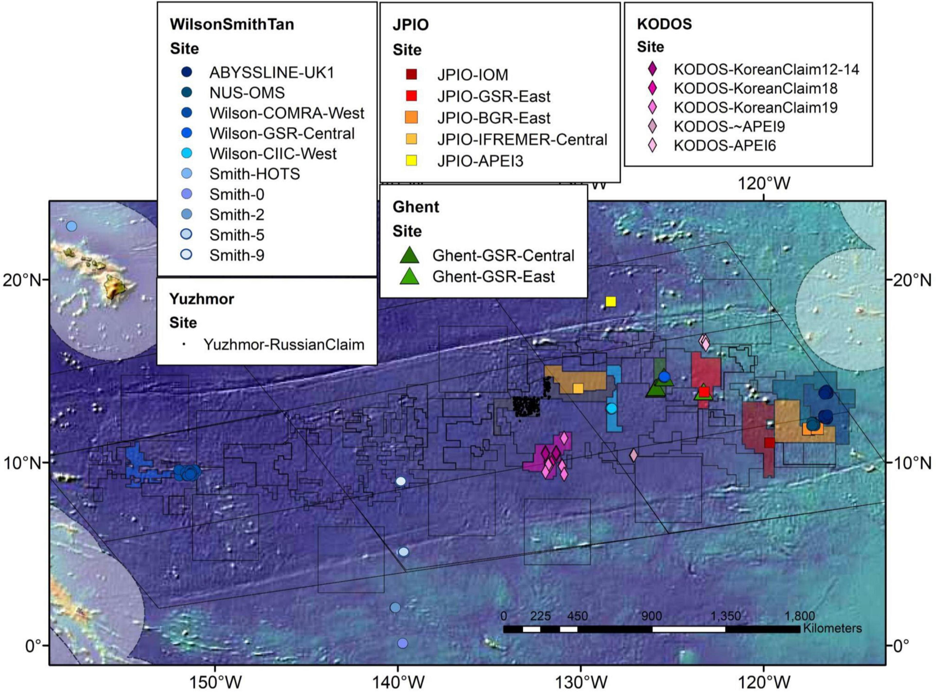
Figure 1. Map of the CCZ showing study sites from which macrofaunal box-core data were assembled for use in this study. The characteristics of the data sets collected at these sites are presented in Tables 1, 2.

TABLE 1

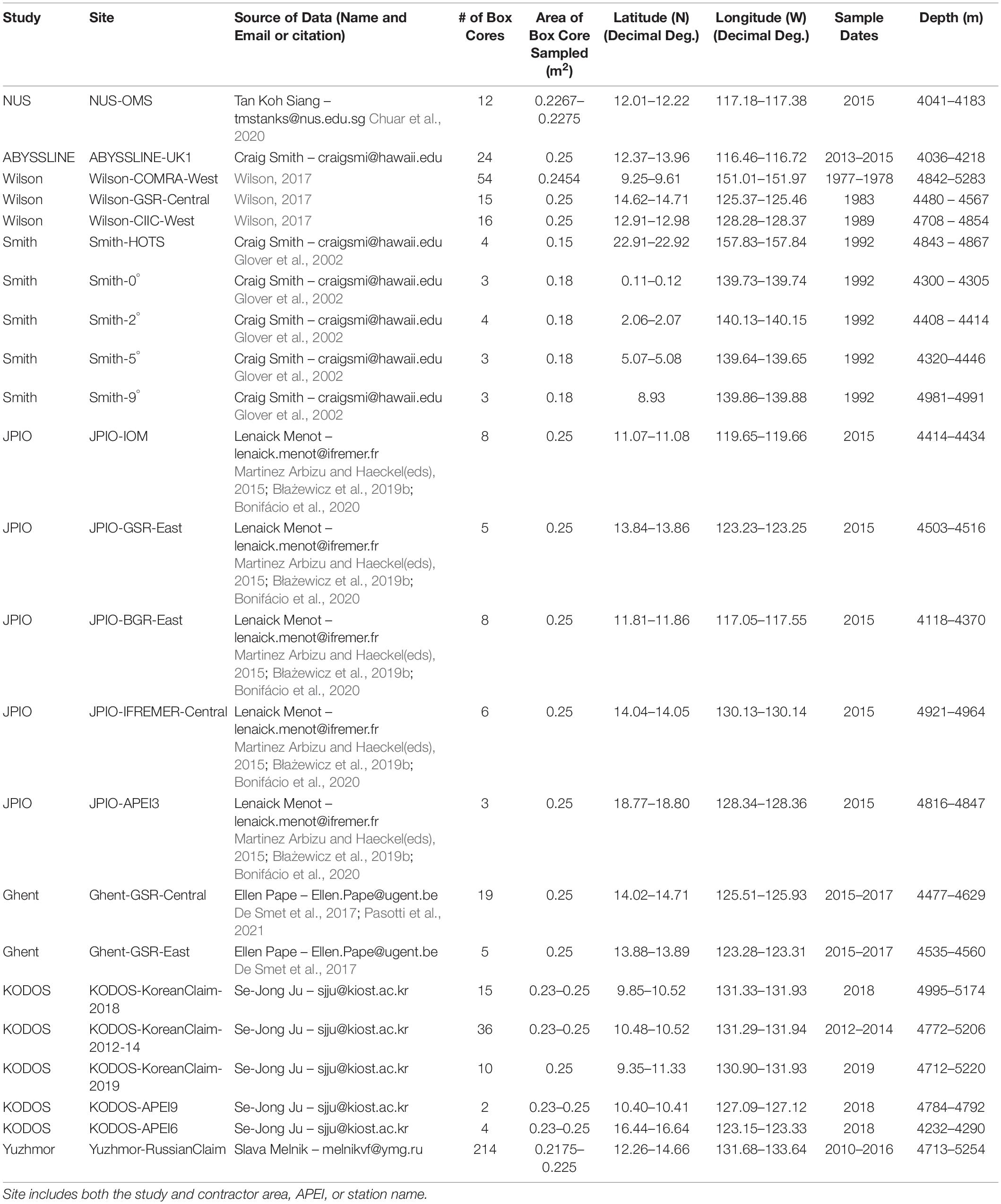
Table 1. Sources, numbers (#) of box cores, locations, and depths for macrofaunal box-core data used in this study.

Data sets were obtained from eight different studies that collected samples from eleven different contractor areas and three APEIs (Glover et al., 2002; De Smet et al., 2017; Wilson, 2017; Błażewicz et al., 2019b; Bonifácio et al., 2020; Chuar et al., 2020; Pasotti et al., 2021). Data sets were obtained from the National University of Singapore (NUS), the Abyssal Biological Baseline Project (ABYSSLINE), multiple projects funded by the National Oceanic and Atmospheric Administration analyzed by Wilson (2017) (Wilson), U.S. Joint Global Ocean Flux Study (JGOFS) (Smith), Joint Programming Initiative Healthy and Productive Seas and Oceans (JPIO) project (JPIO), the Belgian company Global Sea Mineral Resources (GSR) through Ghent University (Ghent), Korea Deep Ocean Study (KODOS), and Yuzhmorgeologiya of the Russian Federation (Yuzhmor) (Figure 1 and Table 1). Macrofaunal data from a total of 477 box cores were analyzed for this synthesis. Sampling sites ranged in depth from ∼ 4000 – 5300 m and were collected between 0 – 23° N and 116 –158° W (data sources and shorthand names for data sets are given in Table 1). Macrofaunal data were compiled for each research group at the site level, i.e., within a contract area or APEI (Figure 1 and Table 1). Most studies differentiated only a subset of macrofaunal taxa (i.e., polychaetes, tanaids, and isopods) to the species level; however, NUS data were resolved only to the family level and Yuzhmor data to the class level (Supplementary Table 1). All studies used a 0.25 m² box corer although some removed small subsamples for other analyses (Table 1). Abundance data for all box-core samples were normalized to 1 m². All studies used 300-μm sieves except for NUS, which used 250-μm. Sampling years ranged from 1977 to 2019 (Table 1).

The Comparability of Box-Core Data Sets

There was substantial variability among “quantitative” box-core data sets in taxa counted and taxonomic resolution obtained. In addition, box-core samples were collected by different research programs (Table 1) using a range of box-core designs, box-core deployment protocols (e.g., lowering speed, stern vs. side A-frame, etc.), and sample-washing procedures (e.g., sieve size, washing-water temperature, on-board vs. in-laboratory sieving, etc.), all of which may influence sampling efficiency and the ability to resolve macrofauna at the species level (Glover et al., 2016). Most macrofaunal box-core data sets distinguished polychaetes, tanaids, and isopods to morphospecies. However, taxonomic and systematic resolution differed among these groups (e.g., many tanaid species were not classified into families), and only one study (ABYSSLINE) distinguished species for all macrofauna collected (Supplementary Table 1).

In addition, the thousands of sediment macrofaunal species in the CCZ are mostly undescribed (Glover et al., 2002; Smith et al., 2008a,b; Glover et al., 2018; Błażewicz et al., 2019b; Jakiel et al., 2019), research programs use different taxonomists with different morphological reference collections to resolve species, and some programs have combined morpho-taxonomy with DNA barcoding (Supplementary Table 1). Since reference collections have not been intercalibrated across all research programs and only a small proportion of macrofaunal species from the CCZ have been DNA barcoded or formally described, we conducted between-site species-level comparisons primarily within research programs to assure consistency in sampling protocols and species-level determinations. However, within one data set (KODOS), box cores collected on different cruises (2012–2014, 2018, and 2019) appear to have different sampling biases, with the percentage of polychaetes resolvable to species level, polychaete abundances, and species/family accumulation curves exhibiting large differences among sampling times; we thus analyzed the KODOS samples as three different data sets. It should be noted that the box-core data sets contributed by Wilson (Wilson), Smith (ABYSSLINE and Smith), and Tan (NUS) were collected and processed with similar protocols [first described in Hessler and Jumars (1974), and more recently in Glover et al. (2016)] by lead personnel trained in a single laboratory (that of R. R. Hessler), so these samples were considered to be a single Wilson–Smith–Tan data set for abundance analyses.

To allow diversity comparisons across data sets, we analyzed patterns at the family level after harmonizing the family level taxonomy using the World Register of Marine Species (WoRMS³).

Analytical Methods

Analyses of the Comparability of Data Sets

Macrofaunal patterns across sites were first explored with regression analyses between macrofaunal abundances and individual environmental parameters, in particular POC flux, nodule abundance estimated from the ISA (2010) Geological Model, and ocean depth. Direct deep POC flux measurements (e.g., from sediment traps) are not available from the study sites considered here. Thus, to explore the relationship between seafloor particulate organic carbon (POC) flux and polychaete abundance, we estimated seafloor POC flux for sampling localities using the Lutz et al. (2007) POC-flux model and the data set created by Lutz et al. (2007), which was calculated for the period 1997 – 2004, an interval near the middle of the range in sampling times (1977–2019) of box cores used in this study; we call these estimates “Lutz POC flux.” The Lutz et al. (2007) POC flux model is trained with sediment-trap data from the CCZ and the equatorial Pacific region generally, and yields results consistent with diagenetic modeling of seafloor POC in the CCZ (Volz et al., 2018). This model has been widely used to evaluate regional patterns of seafloor POC flux in the deep sea (e.g., Sweetman et al., 2017; Snelgrove et al., 2018). Type II regression analyses of polychaete abundance versus Lutz POC flux were performed using linear and exponential functions in Excel, and the function ‘lmodel2’ (Legendre, 2018) in R. The functionality (either linear or exponential) with the highest R² was selected, and ordinary least squares (OLS) regressions were used for all studies since they produced the best fit to the data. Linear mixed-effects modeling, ‘lmer’ (Bates et al., 2015), in R, with “POC flux” as the fixed effect and “Research Program” as the random effect was used to explore the amount of variation explained by POC flux versus study in polychaete abundance. If studies had different sampling efficiencies, we would expect that the “Research Program” effect would explain a relatively high proportion of the variance.

Analyses of Macrofaunal Abundance/Diversity, Environmental Drivers, and Community Structure

Biodiversity patterns were further explored with species and family accumulation curves, Chao 1 species richness estimators, rarefaction, and Pielou’s evenness, as described in Magurran (2004) using EstimateS (Colwell, 2013), R (Venables et al., 2019), or PRIMER 7 (Clarke and Gorley, 2015). Rarefaction curves with 95% confidence limits were calculated in EstimateS for each site by pooling box-core samples within a site. Species accumulation curves and Chao 1 richness were calculated using 100 permutations and the UGE index (Ugland et al., 2003) in EstimateS for each site using box cores as replicates. Pielou’s species and family evenness were calculated in PRIMER 7 for each box core and then averaged within a site. The number of species at each site with abundances of 1 or 2 individuals (singletons or doubletons) was calculated and compared to the total number of species found within each site. A similarity percentages (SIMPER) analysis was used to examine community similarity within study sites while an analysis of similarity (ANOSIM) test was used to examine community differences among sites within a study (Clarke and Gorley, 2015). Finally, the number of species found in more than one contractor area was calculated within studies for “working species,” and across studies for “described species.” “Working species” (i.e., “morphospecies”) have been differentiated by a taxonomist but have not been assigned to a described species (i.e., they are likely new to science); working species are assigned numbers or letters that vary across taxonomists and studies. The number of species shared between sites was explored in the JPIO data set (Błażewicz et al., 2019b; Bonifácio et al., 2020) using UpSet plots generated in R (Conway et al., 2017). UpSet is a technique which visualizes data intersections and sizes of these intersections (Conway et al., 2017).

Linear Mixed-Effects Modeling, ‘lmer,’ in R, was used to explore which environmental variables best explained macrofaunal abundance and taxonomic richness across individual box cores (Bates et al., 2015). Sample depth, Lutz seafloor POC flux (Lutz et al., 2007), nodule abundance (kg/m²) (Morgan, 2012), bottom-water oxygen concentration, bottom-water salinity, bottom-water temperature, bottom-water nitrate, phosphate, and silicate concentrations (all downloaded from World Ocean Atlas 2018⁴; Washburn et al., 2021), bottom slope (largest change in elevation between a cell and its eight neighbors), broad-scale bathymetric position index (BBPI; with an inner radius of 100 km and outer radius of 10000 km) and fine-scale bathymetric position index (FBPI, with an inner radius of 10 km and outer radius of 100 km) (McQuaid et al., 2020) were obtained for each box-core sample location. Since environmental data were not available for many individual locations and several studies, and to ensure data were consistent across studies, data for all environmental variables (except depth, which was provided for each sample) were extracted for each box-core location from interpolated rasters in ArcGis (see Washburn et al., 2021). Environmental variables were standardized, and abundance/richness data were log-transformed to facilitate linearity in the relationship between abundance/richness and environmental variables. If the relationship between an environmental variable and taxon abundance or richness did not appear linear (e.g., appearing parabolic in many cases), a second-order relationship was examined. A linear mixed-effect model was then created with abundance or taxon richness per core as the dependent variable, the standardized environmental variables set as fixed-effect explanatory variables, and site as the random-effect variable. Correlations among environmental variables were explored by calculating the variance inflation factors (VIF) in the ‘car’ package (Fox et al., 2020) and any variables with scores near or above 10 were removed (Montgomery and Peck, 1992). Studies were removed from the model if they appeared to have skewed residuals, and models with all possible combinations of variables were examined using ‘dredge’ in the ‘MuMIn’ package (Barton, 2020). Exploratory analyses found that the majority of variables explained less than 1% of the variation in abundances or richness, so models were refined to include only the variables explaining > 5% of the variance, i.e., depth, Lutz POC flux, nodule abundance, and bottom-water oxygen concentration. Relationships between environmental variables and abundance or richness in the best models, measured by AIC and R² values, were explored further with ANOVAs and regression plots (Zuur et al., 2009).

Community composition for polychaetes at the species level, and for other taxa at the family level, was compared among sites using non-metric multidimensional scaling on square-root transformed abundances/m² in PRIMER 7. SIMPER analysis was then used to explore which taxa were responsible for similarities/differences within and among studies.

Results

The Comparability of Box-Core Data Sets

Because polychaetes typically constituted > 50% of macrofaunal abundance, and polychaete abundance was tabulated in all the box-core data sets, polychaete abundance was used to explore comparability (e.g., sampling efficiency) across research programs. Based on previous abyssal studies of the relationships between seafloor POC flux and macrofaunal abundance (Glover et al., 2002; Smith et al., 2008a; Wei et al., 2010), it was expected that polychaete abundance across the CCZ would exhibit a positive relationship (exponential or linear) with estimated annual seafloor POC flux (Lutz et al., 2007). Abundances per box core spanned an order of magnitude across studies (Supplementary Figure 1), likely in part due to variations in POC flux.

When box-core samples were pooled across all studies, polychaete abundance was exponentially related to POC flux (Figure 2), with 20% of the variation explained. However, the data from individual sampling programs were not evenly distributed above and below the overall regression curve, as would be expected if they were from the same statistical population, with a number of data sets falling largely above or essentially entirely below the curve. This suggests that individual data sets may have different relationships between POC flux and polychaete abundance, as might be expected if sampling protocols (and sampling efficiency) varied among research programs. Furthermore, in the linear mixed effect model including all data with research program as the random effect and POC flux as the fixed effect, the research program effect explained 51% of the variation while POC flux explained 19% (p < 0.0001). This is also consistent with the hypothesis that sampling efficiency varied among research programs.

FIGURE 2

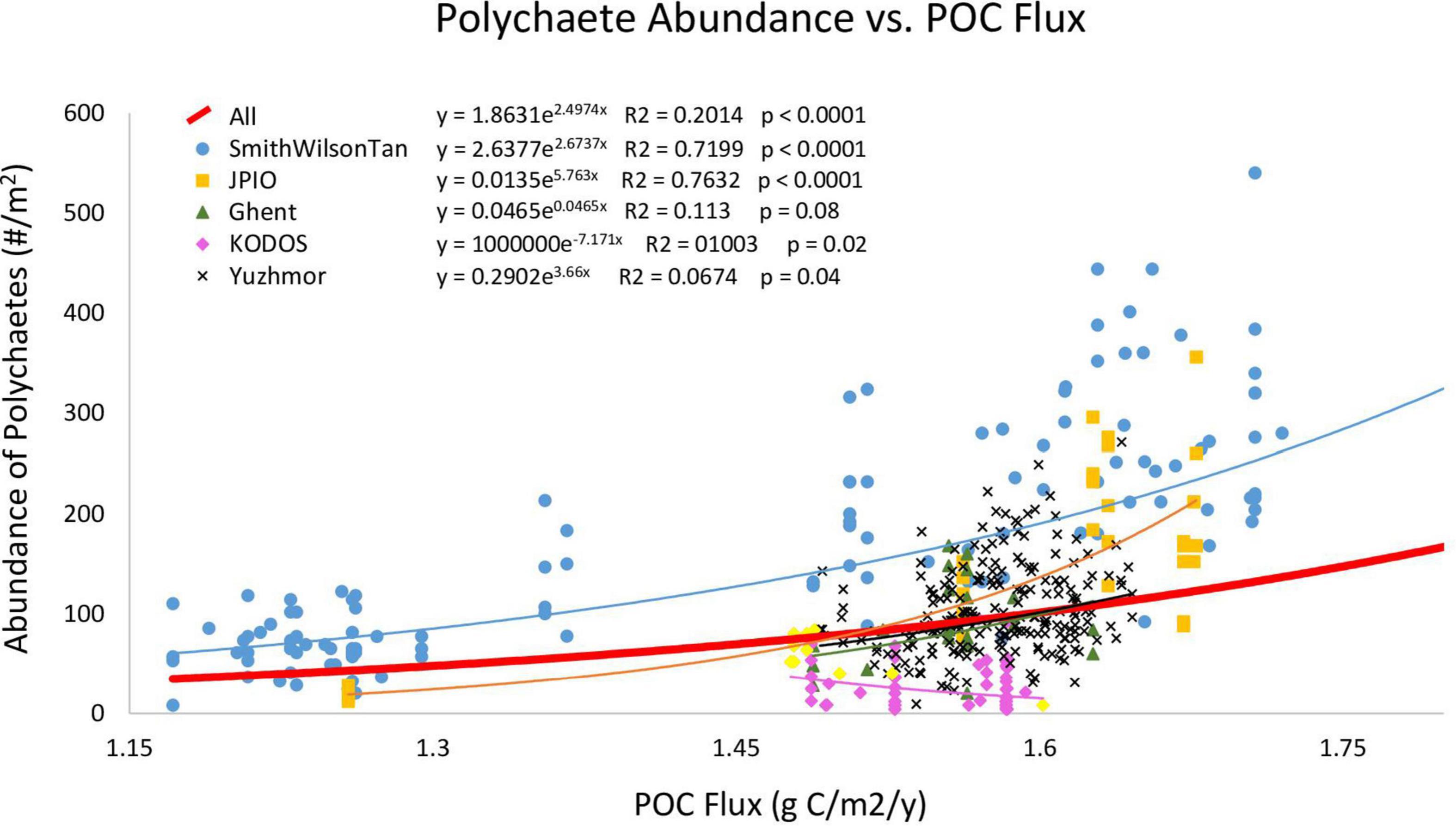
Figure 2. Polychaete abundance in individual box cores versus Lutz POC flux. Curves are Type II regressions conducted in R, with regression equations, R² values, and p levels of regressions indicated. The bold red line is the exponential regression for all sampling programs combined. Regression lines for data sets match the colors of their symbols in the upper left. The pink regression line represents all KODOS data, while yellow diamonds represent KODOS samples collected in 2019. This figure does not show data points for Smith-0, Smith-2, or Smith-5 (which are included in the regressions/curves) as they have much larger POC fluxes and abundances than all other sites making observations of trends for other studies difficult.

We then conducted regressions of POC flux versus polychaete abundance for individual research programs, i.e., studies that were conducted by investigators trained within the same laboratory and thus expected to use similar sampling protocols. The Wilson–Smith–Tan and JPIO studies exhibited positive exponential relationships with high R² values (>0.7), while all other studies, except for KODOS, showed positive but weaker exponential relationships to Lutz POC flux (Figure 2). The KODOS data showed a negative exponential relationship to POC flux, driven largely by relatively low values in box cores collected prior to 2019 (Figure 2), potentially due to differences in sampling protocols, sea states, and/or seasonal/temporal trends in the KODOS area. The Wilson–Smith–Tan data covered the broadest ranges of longitude, latitude and POC fluxes while JPIO data covered the second broadest ranges of these variables (Table 1), providing robust support for the importance of POC flux as an ecosystem driver across the CCZ (cf. Smith et al., 2008a; Wedding et al., 2013; Bonifácio et al., 2020). Due to the differing relationships between polychaete abundance and POC flux across studies, we hypothesized that different studies had different sampling efficiencies and were not directly comparable, so further analyses were performed separately on data sets from individual research programs.

Question 1: Do Abundance, Species/Family Richness and Evenness, and Community Structure, Vary Along and Across the CCZ? What Are the Ecological Drivers of These Variations?

Abundance Patterns

Regional patterns of polychaete abundance

Polychaete abundance showed strong variations along and across the CCZ, including within data sets (e.g., the Wilson–Smith–Tan data in blue and the JPIO data in yellow) (Supplementary Figure 2). Many of the between-site differences are clearly statistically significant, as indicated by the small size of within-site standard errors compared to between-site differences. As noted above (Figure 2), regression analyses indicate that these variations in polychaete abundance across the region are strongly related to Lutz POC flux (Lutz et al., 2007), supporting the use of seafloor POC flux to divide the CCZ management area into ecological subregions (Wedding et al., 2013).

Lutz POC flux explained >70% of the variability in polychaete abundances across the CCZ for two studies and 20% of variability for all studies combined. Regional nodule abundance, when assessed individually with Type II regression, exhibited little relationship with polychaete abundance for all data sets combined, but explained 38 and 48% of variation in the Wilson–Smith–Tan and JPIO data sets, respectively (Figure 3, Smith-0, Smith-2, and Smith-5 not shown). The relationships between depth and polychaete abundance were generally negative, explaining 25% of variability among polychaete abundances when all data sets were combined, and 41 and 35% of abundances for the Wilson-Smith-Tan and JPIO data sets, respectively (Figure 3).

FIGURE 3

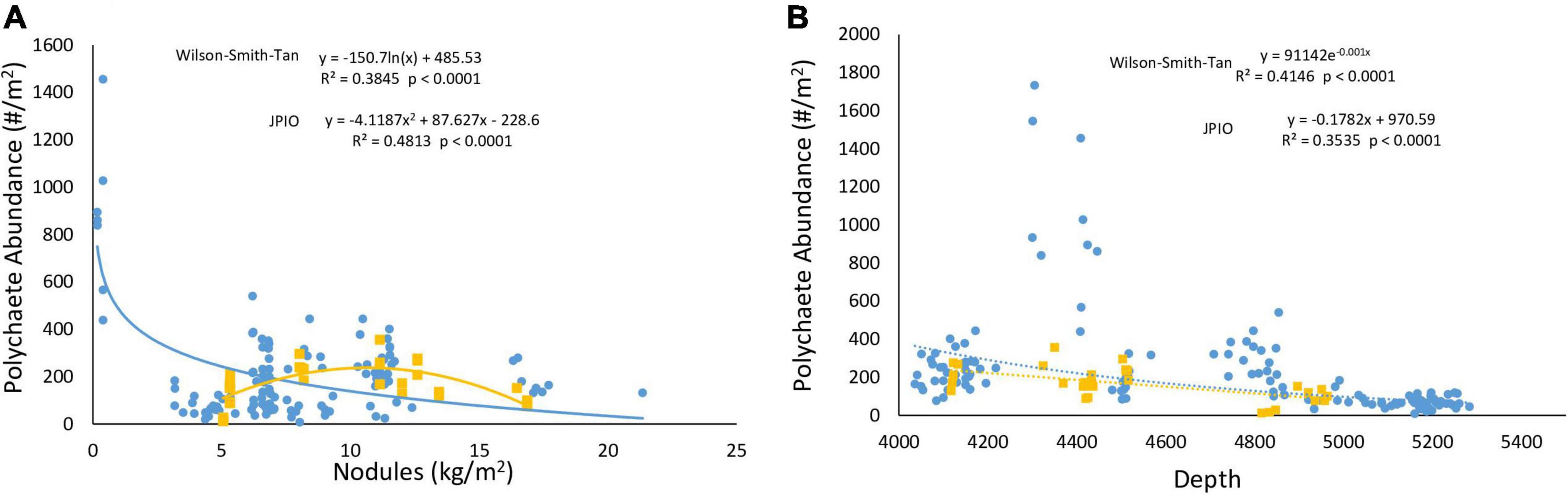
Figure 3. (A) Nodule abundance and (B) depth versus polychaete abundance in the Wilson–Smith–Tan (blue) and JPIO (yellow) data sets. Lines shown are Type II regressions conducted in R. All regressions are highly statistically significant (p < 0.0001).

We also explored the relationship between average polychaete abundance at all sites sampled across the region (Figure 1) versus Lutz POC flux to the seafloor, depth, bottom-water oxygen concentration, nodule abundance, and measures of seafloor slope using linear mixed-effects models. Measures of seafloor slope (i.e., slope, BBPI, FBPI) explained little to no variation in polychaete abundances and were thus removed. ANOVA found that only POC flux had a nearly significant p-value (p = 0.06). Fixed effects (i.e., environmental variables) in the model explained 23% of variation in polychaete abundance when KODOS from 2012 – 2018 and Yuzhmor data (i.e., data sets with very different apparent sampling efficiencies) were excluded. This was almost solely due to POC flux, since the model containing POC flux alone explained 19% of the variation. Neither depth nor nodule abundance explained substantial variation while the inclusion of oxygen concentration actually decreased the R² of the model (Table 2). It is noteworthy that random (study/site) effects explained three times as much variability in polychaete abundance (57%) as the fixed effects, highlighting that there are large differences among sampling programs and/or sites not explained by the current set of environmental variables; these differences are likely caused, at least in part, by differences in sampling efficiency among studies.

TABLE 2

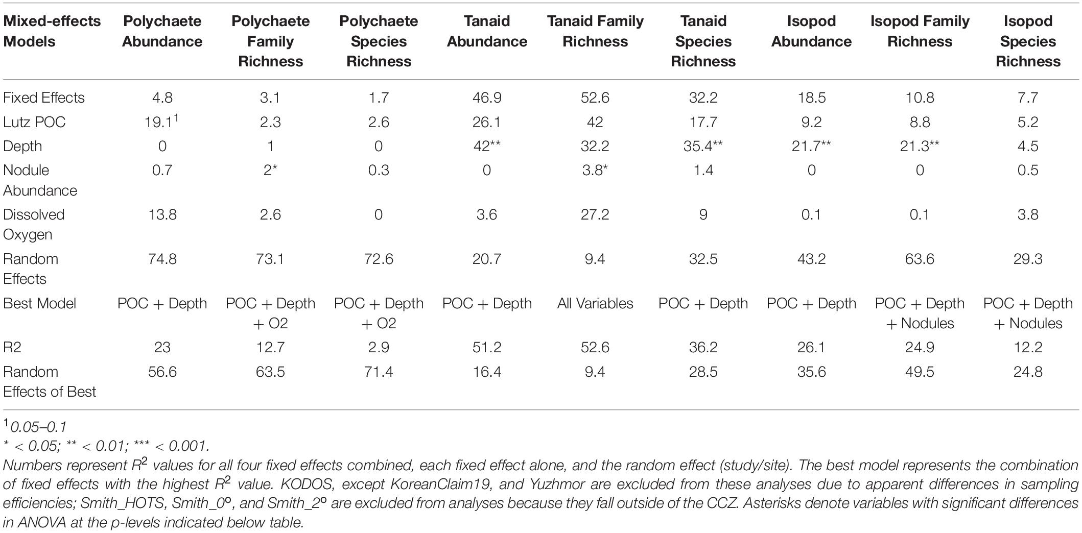
Table 2. Results of linear mixed-effects models examining abundance, family richness, and species richness (taxa within a core) for polychaetes, tanaids, and isopods within the CCZ.

Regional patterns of tanaid and isopod abundance

Regression relationships between tanaid and isopod abundances and Lutz POC flux were similar to those for polychaete abundance. POC flux explained 57 and 47% of variability in tanaid abundances for the Wilson–Smith–Tan and JPIO data sets, respectively, and 26% of tanaid variability for all studies combined. POC flux explained 21 and 17% of variability in isopod abundances for the Wilson–Smith–Tan and JPIO data sets, respectively, and only 7% of isopod variability for all studies combined (Supplementary Figures 3A, 4A). Nodule abundance explained approximately 10% or less of the variation for both tanaid and isopod abundances for all data sets combined as well as for each data set independently, except JPIO; there, nodule abundance explained 27 and 33% of tanaid and isopod abundances, respectively. However, unlike all other studies, the relationships between nodule abundance and polychaete, tanaid, and isopod abundances in JPIO samples were best described by second-order polynomial functions with maximum animal abundances at intermediate nodule abundances (Supplementary Figures 3B, 4B).

Depth explained 31% of variability of tanaid abundances for all data sets combined and 39 and 47% of abundances for the Wilson–Smith–Tan and JPIO data sets, respectively. Depth exhibited little relationship with isopod abundances for all data sets combined. Depth explained 27, 43, and 47% of variability of isopod abundances for the Wilson–Smith–Tan, JPIO, and Ghent data sets, respectively. However, unlike polychaetes and tanaids, regression relationships for isopod abundances were best represented by second-order polynomial functions with maximum abundances at intermediate depths for Wilson–Smith–Tan, but with minimum abundances at intermediate depths for JPIO and Ghent. Measures of slope explained little to no variation in tanaid or isopod abundances (Supplementary Figures 3C, 4C).

Overall, these regression relationships suggest that on regional scales across the CCZ, POC flux, and to lesser degrees nodule abundance and depth, are likely to be important drivers of tanaid and isopod abundances. The differences in these relationships among studies and the lack of relationships to POC flux, nodule abundance, and depth for the Ghent, KODOS, and Yuzhmor data sets further suggest differences in sampling efficiencies among studies. These differences may also be due in part to the narrow range of variation among explanatory variables in the above data sets due to their limited geographical extents.

Linear mixed-effects models for both tanaid and isopod abundance indicated that environmental variables were important, with fixed effects explaining over 50% of the variability in tanaid abundances and 25% for isopod abundances in the best models. ANOVA indicated that depth was significant for both tanaids (p = 0.004) and isopods (p = 0.006). The inclusion of oxygen and nodule abundance in either model decreased its ability to explain variations in abundances. For both tanaids and isopods, depth alone explained nearly all the variability attributed to fixed effects. POC flux explained roughly half of the variability in either model (tanaids ∼25%, isopods ∼10%). Removal of POC flux did not appear to affect the quality of the model when depth was left in, suggesting that half of the variability related to depth may be caused by covarying POC flux. Nodule abundance explained 0% of the variability for either tanaid or isopod abundance (Table 2).

Biodiversity Patterns at the Species Level

Polychaetes

All sites with species-level, box-core data for polychaetes exhibited rising species accumulation curves, in many cases with steep slopes and with none approaching a plateau (Figure 4). These curves indicate that polychaete species richness at all sites remains under-sampled, i.e., species are still accumulating rapidly and additional sampling at any site will collect previously unsampled species, even when large numbers of box cores have already been collected (e.g., >50 at COMRA-West; Table 1). The rapidly rising curves reflect the fact that many/most species at each site are rare; >49% of species were singletons or doubletons, i.e., represented by only one or two individuals, in the pooled samples from any site (Figure 5). Within internally consistent data sets (e.g., within the Wilson and within the JPIO data sets), there are substantial between-site differences in the slopes and apparent asymptotes of species accumulation curves (Figure 4).

FIGURE 4

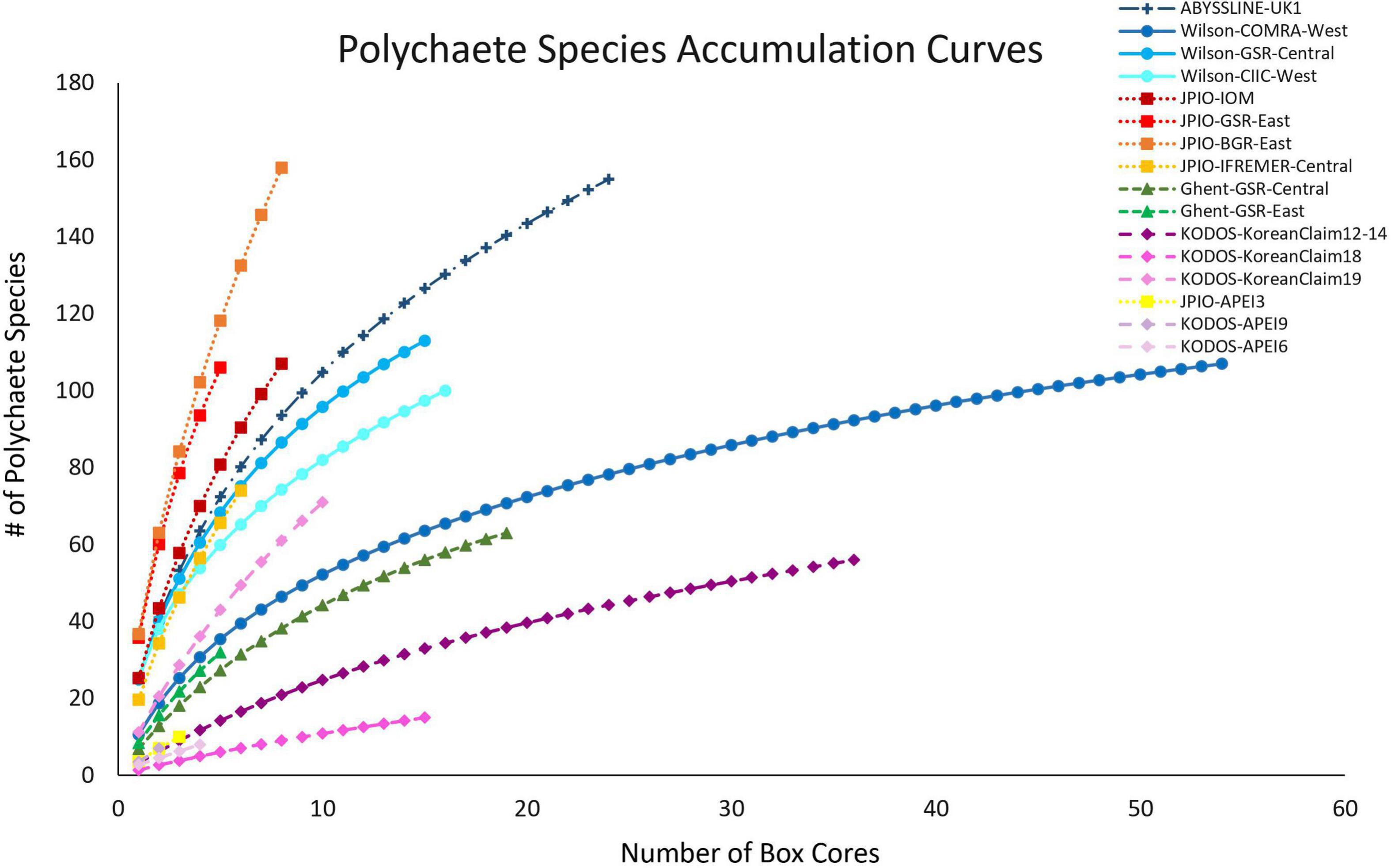
Figure 4. Mean polychaete species accumulation as a function of number of box-core samples (UGE plot from EstimateS, 100 permutations) at different sites in the CCZ region. Note that KODOS-KoreanClaim data come from a single site sampled in different years. Data sets that are considered to have been sampled with similar protocols and to have used a consistent taxonomy are indicated by similar symbols.

FIGURE 5

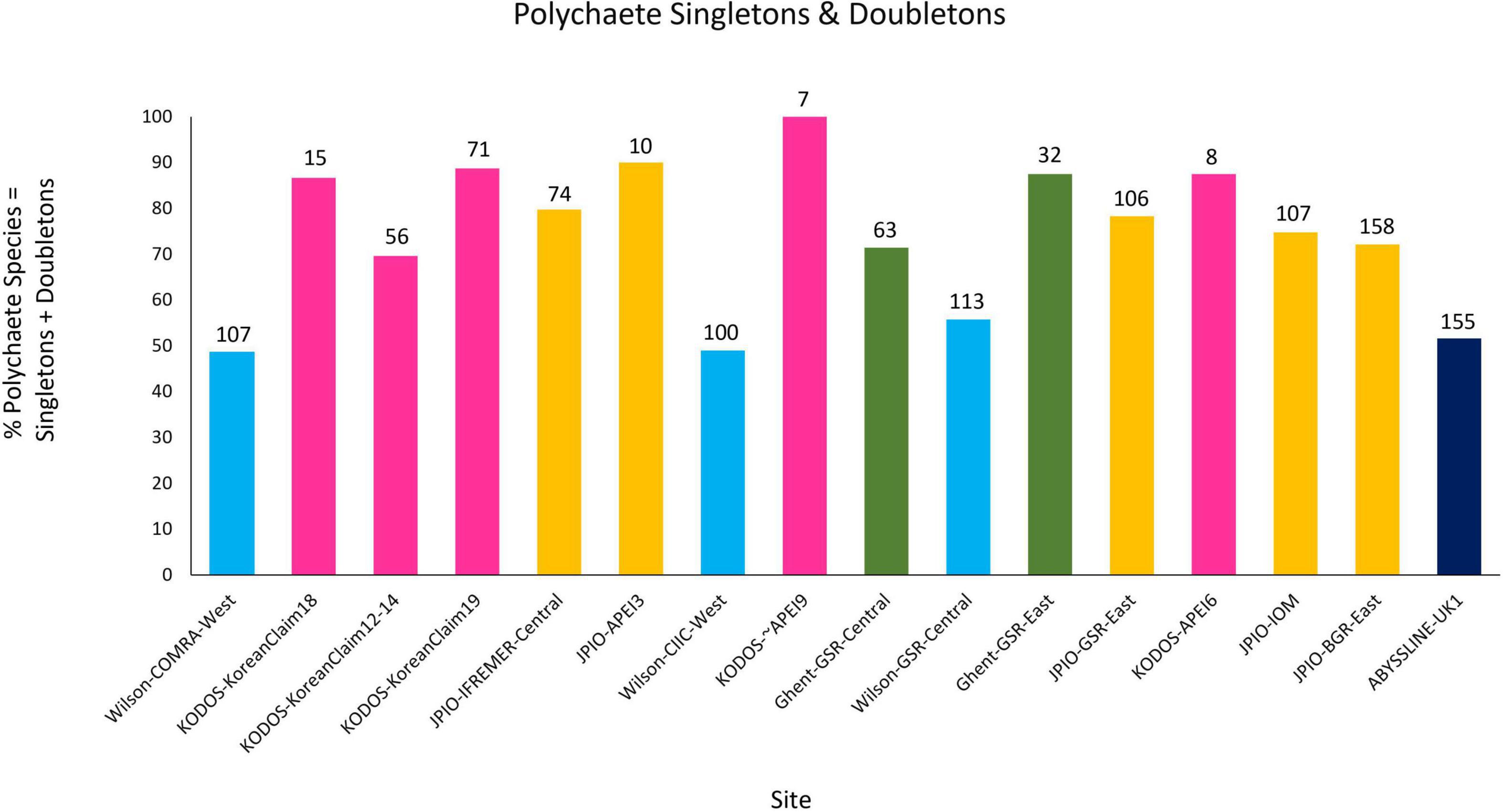
Figure 5. Percentage of total polychaete species represented by singletons + doubletons in pooled collections from each site and study. The total number of polychaete species collected in each data set is indicated at the top of each bar. Note that KODOS-KoreanClaim data come from a single site sampled in different years, and potentially with different sampling efficiencies. Data sets considered to have been sampled with similar protocols and to have used a consistent taxonomy are indicated by similar colors.

Because species were still accumulating at all sites, the Chao 1 statistic (Figure 6) was used to estimate the total number of species expected to be collected at each site (Magurran, 2004). Chao 1 estimates range from ∼25 to ∼370 species, with all the relatively well-sampled sites estimated to have > 100 species of polychaetes. Estimated total species richness at all sites substantially exceeds the number of species collected, i.e., only 25 – 73% of estimated polychaete species richness has been recovered at any site (Supplementary Figure 5). It is important to note that for many sites (ABYSSLINE-UK1, Wilson-CIIC-West, all five JPIO sites), the Chao 1 curves are increasing rapidly with additional box cores (Figure 6) suggesting that at these sites, estimated species richness will increase substantially with additional sampling (i.e., the current Chao 1 number is an underestimate). Species diversity (including richness) can only be directly compared between those sites with a common polychaete taxonomy (i.e., internally consistent species differentiation), and only one internally consistent box-core data set, JPIO, has sampled > 3 sites (n = 5) across a substantial range (1400 km) of the CCZ (Figure 1; Bonifácio et al., 2020). The JPIO data (based on morphological and molecular differentiation of species) indicate substantial variability in species richness across sites (Supplementary Figure 5), which appears to be driven by differences in POC flux and nodule abundance (Bonifácio et al., 2020).

FIGURE 6

Figure 6. Chao 1 (+SD) estimates of polychaete species richness as a function of number of box cores collected at 16 sites across the CCZ region. Note that KODOS-KoreanClaim data come from a single site sampled in different years. Data sets considered to have been sampled with similar protocols and to have used a consistent taxonomy are indicated by similar symbols.

Individual-based species rarefaction curves for all sites exhibit similar initial slopes (with overlapping 95% confidence limits) suggesting similar, high levels of species evenness across sites (Supplementary Figure 6). However, rarefaction diversity at higher numbers of individuals, i.e., toward the right ends of curves and at Es₍₁₃₀₎, exhibit significant variability across sites within data sets (Figure 7 and Supplementary Figure 6). These between-site differences in rarefaction diversity were not strongly related to POC flux (Supplementary Figure 6), in agreement with the findings of Bonifácio et al. (2020) for the JPIO data set.

FIGURE 7

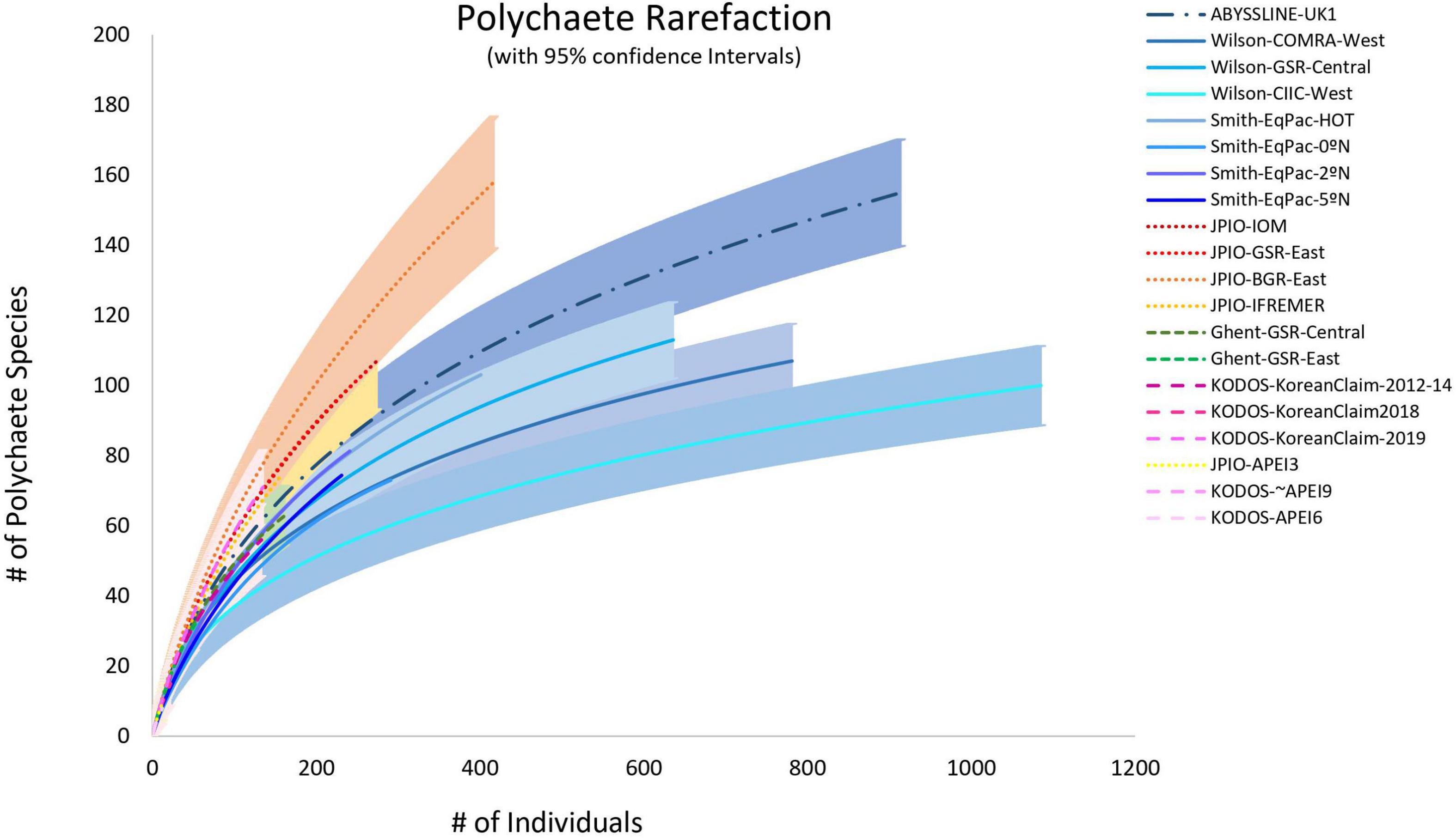
Figure 7. Individual-based polychaete species rarefaction curves by site. Envelopes indicate 95% confidence limits for curves. Note that the KODOS-KoreanClaim data come from a single site sampled in different years. Data sets considered to have been sampled with similar protocols and to have used a consistent taxonomy, are indicated by similar line types.

Mean Pielou Evenness J’, calculated at the box-core level, was generally high (near 1.0) and showed little variation across sites, except that the Wilson-CIIC-West site value was unusually low (∼0.9) (Supplementary Figure 7). Overall, this result is consistent with the similarity of initial slopes of species rarefactions curves in Figure 7.

No environmental variables in the linear mixed-effects model for polychaete species richness per core were significant in ANOVA. The fixed effects (POC flux, Depth, O₂, and nodule abundance) explained less than 5% of species richness. On the other hand, the random variable explained over 70% of richness differences (Table 2), suggesting that differences in sampling efficiency and taxonomy among research programs may have contributed to differences in species richness among studies.

The similarity of polychaete communities among box cores from single studies, measured by SIMPER, ranged from 0 to 49%. ANOSIM tests found communities differed significantly among the three sites in the Wilson data set and the five sites in the JPIO data set. Generally, communities at sites further away were more different. However, evenness and the proportion of species represented as singletons are high, which means that samples with few individuals are likely to be dissimilar to other samples. For the Wilson data set, communities at GSR-Central and CIIC-West clustered together vs. COMRA-West, but abundances were also lower in COMRA-West vs. the other sites. Samples from COMRA-West appeared to have decreasing similarity with decreasing abundance (Supplementary Figure 8). A similar trend was observed in samples from the JPIO data set, with IOM, BGR-East, and GSR-East clustered together and different from Ifremer, which had lower abundances per sample than the other three sites (Supplementary Figure 8).

Tanaids and isopods

Rapid rates of species accumulation were observed across all sites for tanaid and isopod crustaceans, as for polychaetes, indicating that these crustacean assemblages remain poorly sampled (Figure 8). As for polychaetes, large proportions of the species at all sites (>45%) were represented by singletons + doubletons, and a substantial percentage of Chao-1 estimated species richness remained uncollected (>15%), indicating that these assemblages are incompletely sampled, even with >50 box cores (Wilson-COMRA-West). Within data sets, there was some heterogeneity between sites in accumulation curves and estimated species richness (Figures 8, 9). Estimated total species richness at most sites substantially exceeds the number of species collected for both tanaids and isopods with only 16–85% of estimated tanaid species richness, and 20–80% of isopod richness, recovered at any site (Figure 9). Unlike polychaetes, individual-based species rarefaction curves for tanaids exhibit similar curves across most sites. Only one data set, Wilson, collected more than 30 isopods at two or more sites, and rarefaction curves for these three sites were similar as well (Supplementary Figure 9).

FIGURE 8

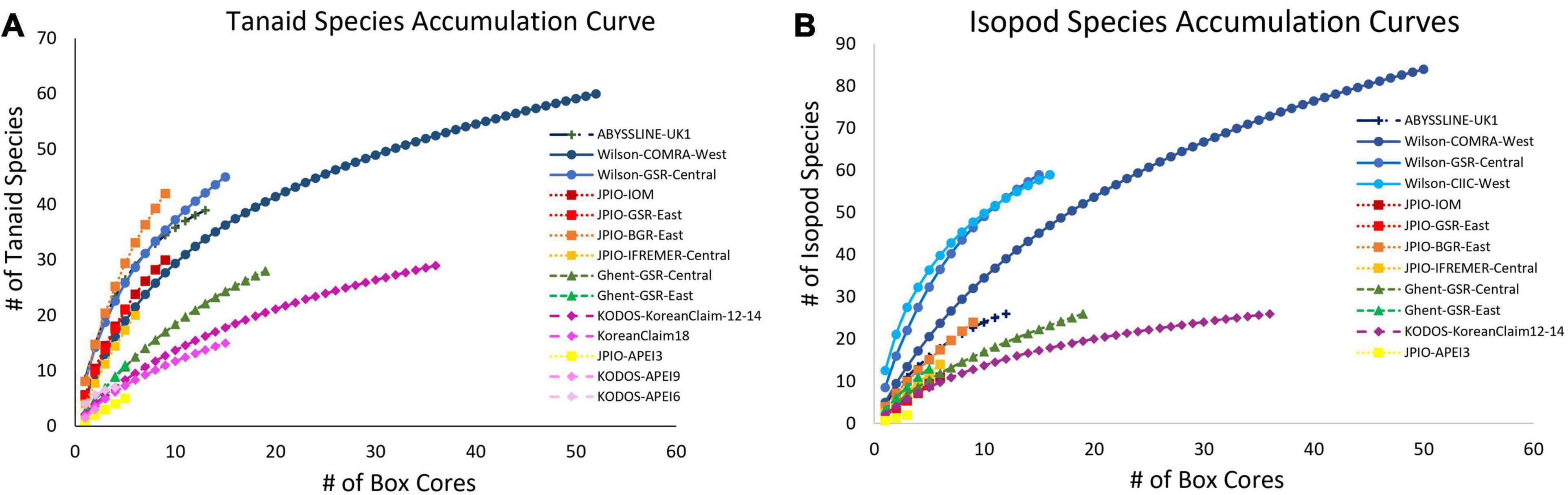
Figure 8. Mean (A) tanaid and (B) isopod species accumulation as a function of number of box-core samples (UGE plot from EstimateS, 100 permutations) at different sites in the CCZ region. Note that the Korean Claim data come from a single site sampled in different years. Data sets considered to have been sampled with similar protocols and to have used a consistent taxonomy, are indicated by similar symbols.

FIGURE 9

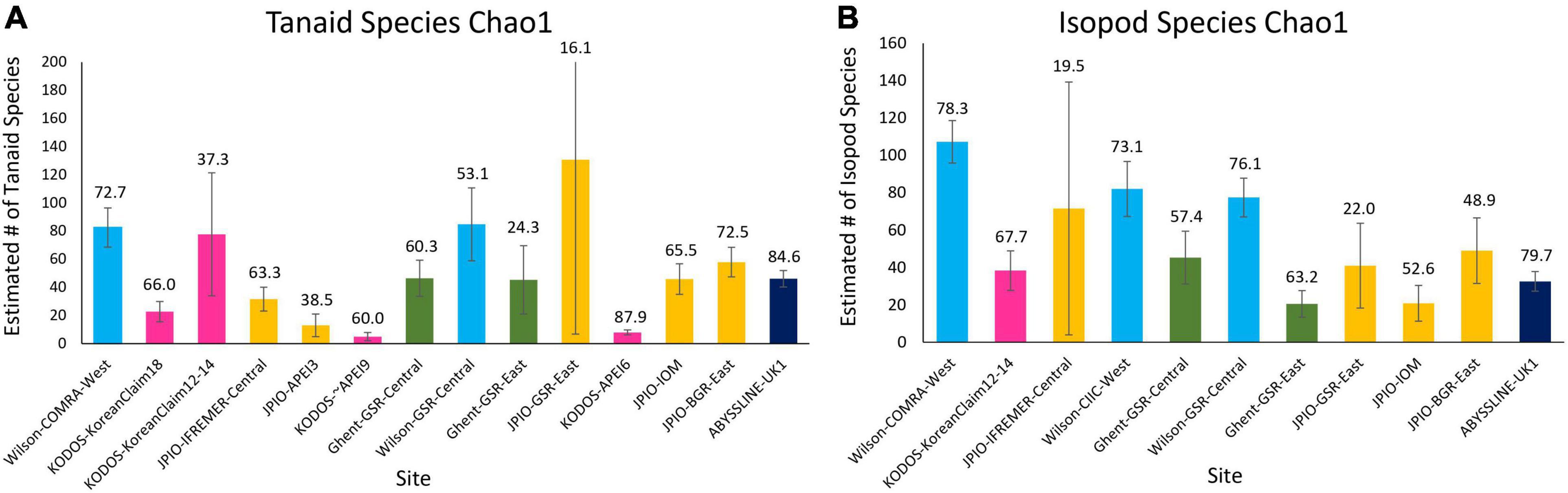
Figure 9. Chao 1 (+SD) estimate of species richness for (A) tanaid and (B) isopod assemblages at the various sites sampled across the CCZ. Numbers over bars indicate the percentage of estimated species richness that has been collected at each site.

Unlike polychaete species richness, the fixed (environmental) effects in the best mixed effects model for tanaid species richness explained over 35% of variation. ANOVA results for this model show a significant difference for depth, and nearly all the variation explained in the model was attributed to depth. POC flux explained roughly half of the variation in tanaid richness as depth, suggesting that half of the apparent influence of depth on tanaid richness is due to POC flux. Nodule abundance explained less than 2% of variation. The fixed effects in the mixed effects model for isopod species richness explained roughly 10% of variation while ANOVA results showed no significant differences in any environmental variables for this model (Table 2). The random effect explained over 30% of variation in tanaid species richness and over 40% in isopod species richness, again suggesting that differences in sample efficiency inhibit comparisons across studies.

Within study sites, community similarities at the species level among tanaid communities, based on SIMPER, ranged from 0 – 24%, and from 0 – 28% among isopod communities. ANOSIM analyses found communities differed significantly among all study sites in the Wilson data set for both tanaids and isopods, and in the JPIO data set for tanaids. nMDS plots separated sites in the Wilson data set for isopods but not for tanaids, while JPIO sites were spatially separated for tanaids and isopods (with very low abundances, Supplementary Figures 10, 11). As for polychaetes, much of the dissimilarity appeared to be directly related to samples with small numbers of individuals.

Biodiversity Patterns at the Family Level

To minimize differences in taxonomy among data sets, we also explored patterns of diversity and community structure at the family level. Identifications at the family level are generally standardized across taxonomists and sampling programs, and the sampling of families is usually more complete and less biased than sampling of many hundreds of rare, undescribed species. For older data sets (e.g., Wilson, 2017), we updated family classifications to the current family taxonomy using WoRMS.

Polychaetes

For most sites with >10 box-core samples, polychaete family accumulation curves were leveling off (Figure 10), and the number of families collected was generally > 80% of Chao-1 family richness estimates (Supplementary Figure 12), suggesting that most sites are well sampled for polychaete families. There was substantial across-site variability in estimated family richness, both within and across sampling programs.

FIGURE 10

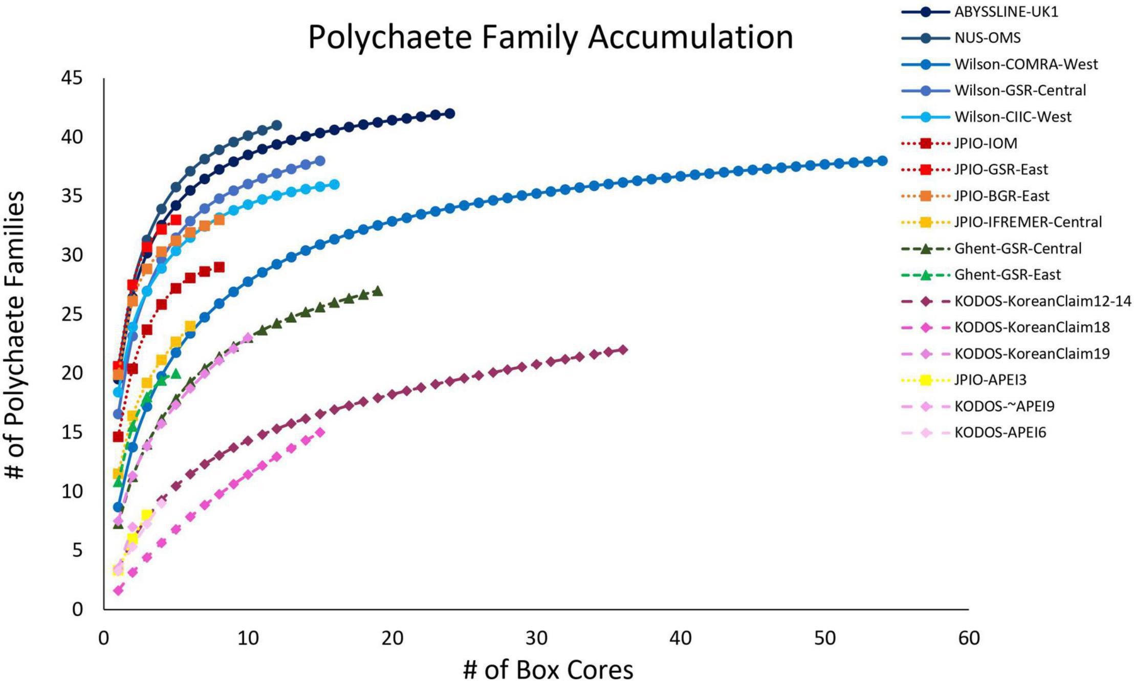
Figure 10. Mean polychaete family accumulation versus number of box-core samples (UGE plot from EstimateS, 100 permutations) at different sites in the CCZ region. Note that KODOS data come from a single site sampled in different years. Data sets considered to have been sampled with similar protocols are indicated by similar symbols.

A linear mixed-effects model exploring the relationship between polychaete family richness per core and four explanatory environmental variables (Lutz POC flux, depth, nodule density in kg/m², and bottom-water oxygen concentration) found that fixed effects in the best model explained approximately 15% of variation in family richness, but only nodule abundance was statistically significant (p < 0.05) and explained only 2% of the variation. The random effect explained over 60% of the variation (Table 2). Thus, differences in sampling efficiency or unmeasured environmental, or biotic, variables may be largely driving differences in polychaete family richness per core among the study sites.

Community structure at the family level also differed across sites, with some carnivorous families (e.g., lumbrinerids and goniadids) being relatively common at sites with higher POC flux and rare or absent from sites with low POC flux (Figure 11, purple and brown wedges). While both lumbrinerids and goniadids were almost completely absent at sites with the lowest POC fluxes, lumbrinerids exhibited a positive linear relationship with POC flux while goniadids exhibited a parabolic relationship with POC flux with highest abundances at intermediate levels (Supplementary Figure 13). However, p-values for both lumbrinerids and goniadids relationships with POC flux were not significant.

FIGURE 11

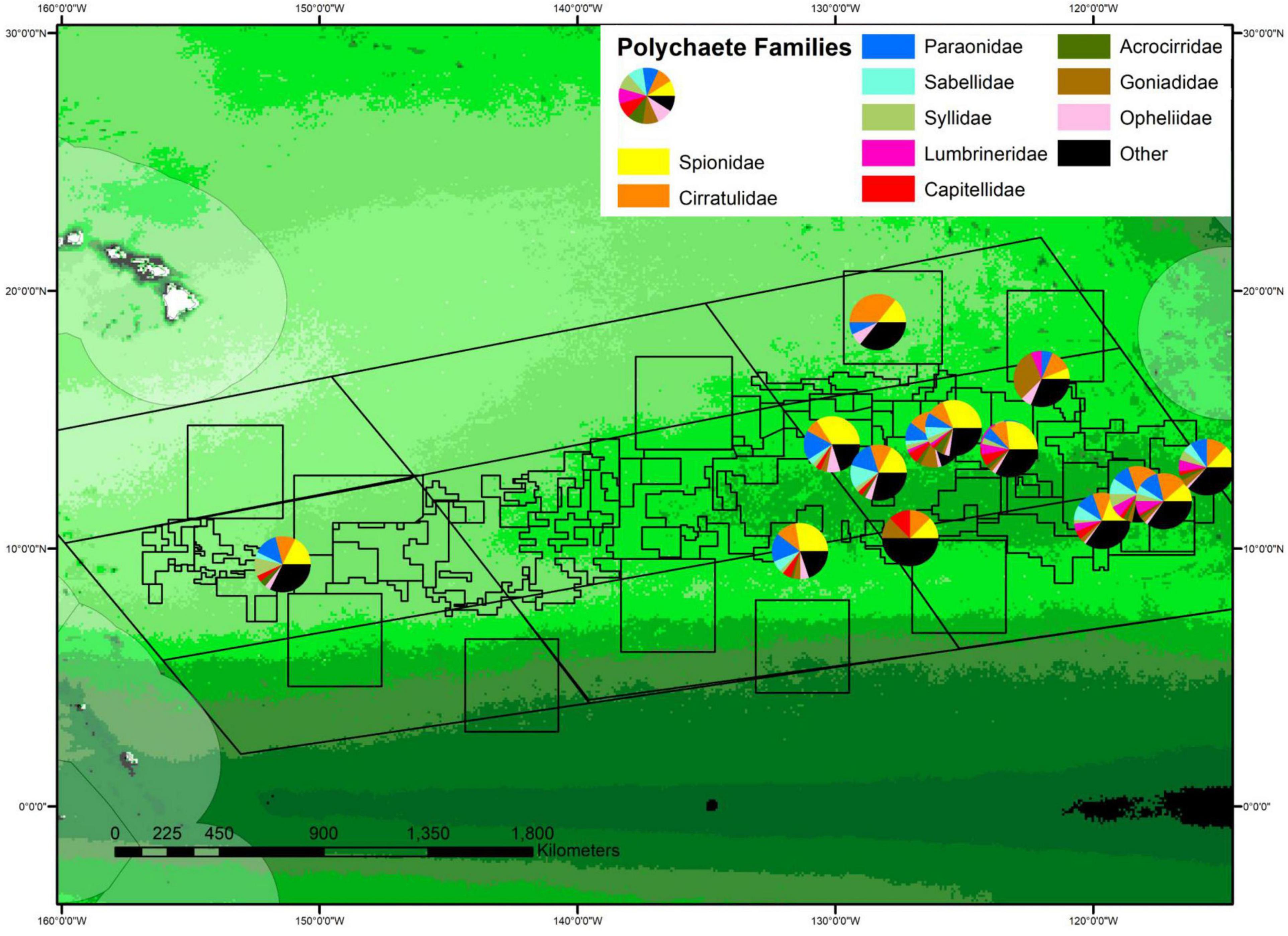
Figure 11. Percent composition of polychaetes by family plotted on the regional map of POC flux. The percent abundance of the 10 most common families is shown, with the size of wedges of circles proportional to percent abundance. The center of each chart in the map indicates site location, with some offsets to allow all pie charts to be visible. See Supplementary Figure S2 for POC flux scale.

Question 2: Do Claim Areas Have Similar Levels of Species/Taxon Richness and Evenness, and Similar Community Structure, to the Proximal APEI(s)?

The sediment macrofaunal data from APEIs are extremely limited, with only APEI 3 sampled within its core region (at a single site) with three box cores, and single sites on the edges of APEIs 6 and 9 sampled with four and two box cores, respectively. Polychaete community abundance, and Chao 1 species and family richness were substantially lower in the core of APEI 3 than in license areas 600 – 900 km away (IFREMER-Central and GSR-East) sampled during the JPIO program (Supplementary Figures 2, 5, 12). These differences appear to be related to lower POC flux and nodule abundance in APEI 3 (Figure 2) (Bonifácio et al., 2020). Polychaete abundance and Chao 1 species richness were also lower on the edges of APEI 6 and 9 than in the KODOS area 600 –1200 km away sampled during the same cruise (Supplementary Figures 2, 5). These differences may also be related to differences in POC flux.

Species level comparisons between APEIs and contract areas are very problematic because so few macrofaunal individuals were collected in/near APEIs (e.g., only 13 polychaete, 5 tanaid, and 2 isopod individuals in APEI 3). Six of the 10 polychaete species found in APEI 3 were not found at any other JPIO site. In fact, only one species (Aphelochaeta sp. 2062) was found in more than one core in APEI 3, making it impossible to characterize macrofaunal communities from these samples. There were only five tanaid species and two isopod species collected in APEI 3 (all singletons) with one species of each crustacean taxon found at additional JPIO sites.

At the polychaete family level, nMDS analyses show all three sites inside or near APEIs as outliers in community structure compared to sites sampled within license areas (Figure 12). However, these differences could well be caused by the very limited number of box cores (3 – 4) and polychaetes (<16) collected in or near the APEIs. It is noteworthy that KODOS 2018, which also has very few polychaetes identifiable to family level (n = 28), is an outlier compared to the sites with larger samples. For tanaid families, APEIs 3 and 9 appear as outliers, but, once again, these sites are very poorly sampled with <4 tanaids identified to family. Both sites in the Wilson data set also had very different tanaid communities than all other studies; however, these individuals were identified ∼ 40 years ago and the family level taxonomy of tanaids has been revised since that time. While we updated tanaid families using the current taxonomy in WoRMS, tanaid species in Wilson were only identified by number so may not have been assigned reliably to current tanaid families.

FIGURE 12

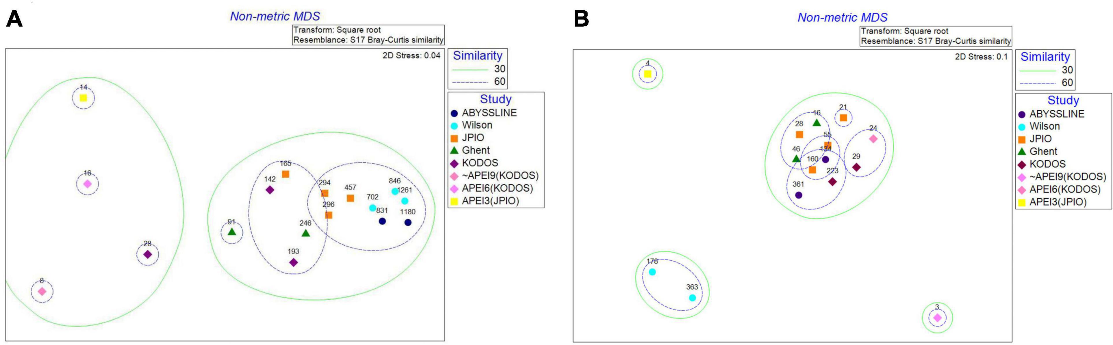
Figure 12. NMDS plots of (A) polychaete and (B) tanaid family community structure for contractor areas and in or near APEIs. Dashed lines bound sites with 30 and 60% similarity. Numbers above points represent the number of individuals collected at each site.

Question 3: Are Species Ranges (Based on Morphology and/or Barcoding) Generally Large Compared to the Distances Between APEIs and Contractor Areas? What Is the Degree of Species Overlap Between Different Study Locations Across the CCZ?

Distribution of Described Polychaete Species Among Box-Core Studies

For the purpose of this analysis we assume that described species can be consistently identified across taxonomists, although that is not necessarily the case. There were 54 described species of polychaetes identified in our combined macrofaunal data set. Some of these identifications included “cf.”, i.e., to be compared with a given described species. Again, for the purpose of this analysis, we assume that individuals identified with a “cf.” belong to the referenced species. Thirteen of the 54 identified species were found at more than one contractor site. Eleven species were shared between the Korean Claim and UK1, and seven species were shared between GSR and UK1. Two species were found in the BGR, GSR-East, GSR-Central, IFREMER, UK1, and Korean claim sites as well as APEI 6. These two species, the spionid Aurospio cf. dibranchiata and the goniadid Bathyglycinde cf. profunda, were the most commonly collected described species in the CCZ data set and have been found in other ocean basins (Maciolek, 1981; Mincks et al., 2009; Boggemann, 2016). Aurospio cf. dibranchiata, Bathyglycinde cf. profunda, Ceratocephale cf. regularis, Levinsenia cf. uncinata, Paralacydonia cf. paradoxa, Paraonella abranchiata, Prionospio branchilucida, Progoniada cf. regularis, Pseudomystides rarica, and Terebellides cf. abyssalis were found at sites separated by 1500 – 2000 km (Supplementary Figure 14). However, one polychaete species (Lumbrinerides cf. laubieri) represented by many individuals (68) was identified from stations within only one site separated by ∼200 km. Thus, three-quarters of the described polychaetes, including one collected many times, were sampled from only a small geographic range (≤200 km) while some commonly collected polychaete species show evidence of broad geographic ranges (Supplementary Figure 14). Among the fourteen described species of tanaids (Błażewicz et al., 2019a; Jakiel et al., 2019), only one (Stenotanais arenasi) was found at more than one study site; this was the only described tanaid species for which numerous individuals (16) were collected (Supplementary Figure 14) while there were no described species of isopods.

Distribution of “Working Species” Within Box-Core Studies

The JPIO study included the largest number of different sites and spans ∼1400 km (Figure 1), although all the JPIO sites are in the eastern CCZ. Roughly 30% of working species of polychaetes and 5 – 10% of tanaid and isopod working species in the JPIO data set range over 600 – 1200 km, with four polychaete and one tanaid species occurring in APEI 3 and contract areas separated by 1250 – 1400 km (Figure 13). However, roughly 60% of polychaete, 80% of tanaid, and nearly 90% of isopod species were found only at single sites, with 60 – 80% of species found at only one site as singletons (Figure 13).

FIGURE 13

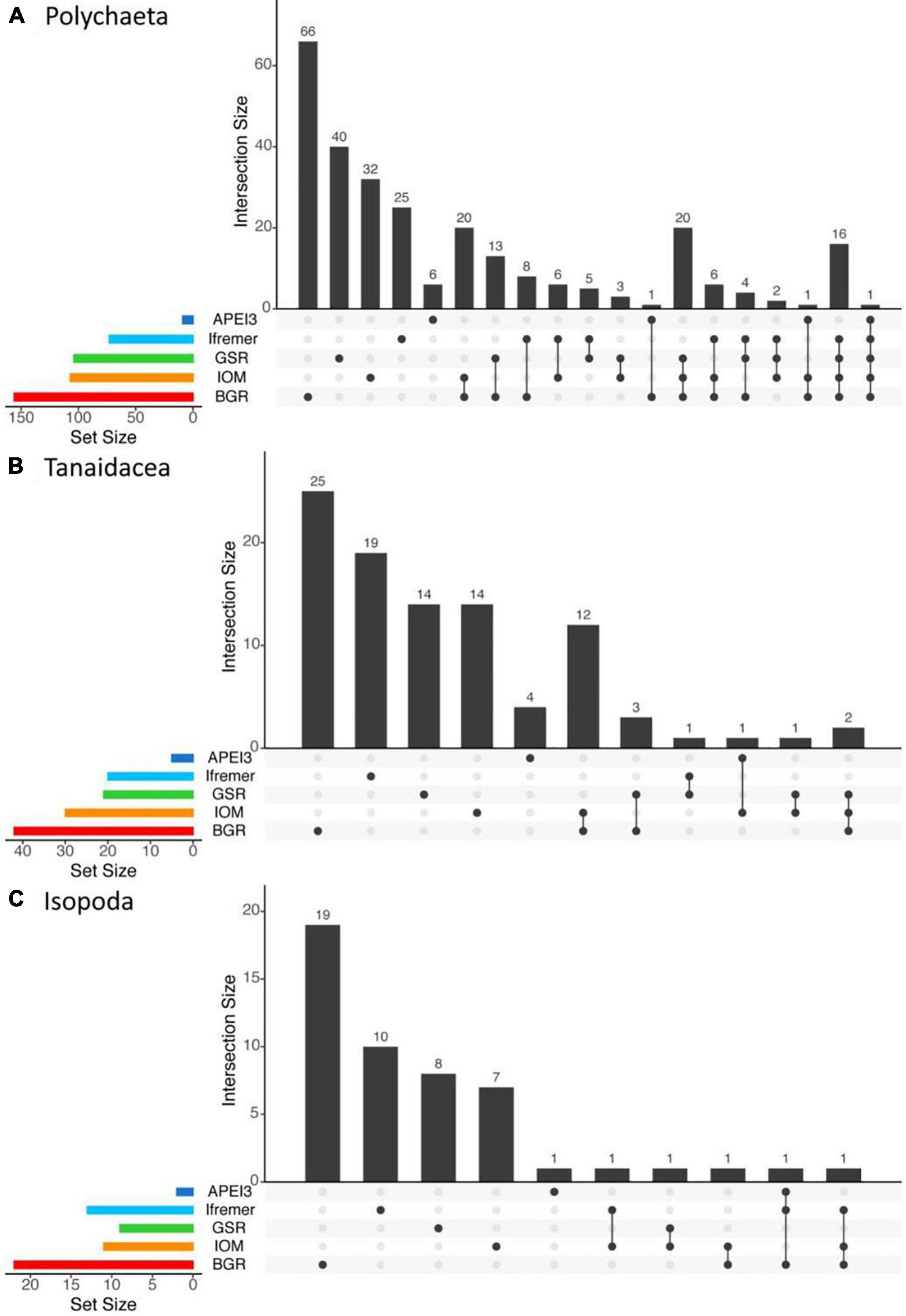
Figure 13. UpSet plots showing the intersection of sediment macrofaunal species resolved by morphological and/or molecular approaches across the five JPIO sites (i.e., sites with a common species-level taxonomy) for (A) polychaetes, (B) tanaids, and (C) isopods. Vertical bars on the main plots represent the number of the unique species in each area (indicated by dots in the bottom part of the graph) or number of species shared across sites (dots connected by lines). Bars on the left are the total number of morphological species and MOTUs (Molecular Operational Taxonomic Units) identified in each of the five areas.

These results suggest that the ranges of some relatively common macrofaunal species are broad, while many other species, including some with high local abundance, may have small ranges compared to the size of exploration contract areas (up to 75000 km²) and the distance from contractor areas to the nearest APEIs (often 100s of kilometers). However, because most macrofaunal species sampled are rare, it is very difficult to distinguish whether species typically are endemic to single sites (i.e., have small ranges compared the spacing of samples across the region, Figure 1), or are present but not yet sampled at multiple sites.

Discussion

Our analyses of abundance patterns of polychaetes (which dominate the macrofauna), tanaids and isopods strongly suggest the hypothesis that different sampling programs have had differing sampling efficiencies for macrofauna, although spatial and temporal variations in ecological drivers likely also have contributed to variations among studies. Differing sampling efficiencies were indicated by regression analyses of polychaete abundance versus POC flux, and as random effects in our linear mixed models for multiple taxa. Variations in sampling efficiencies may be caused by differences in box-coring equipment, lowering protocols, characteristics of ship motion, deployment locations (e.g., stern versus side A-frames), and sample-washing and preservation protocols (Glover et al., 2016). These potential differences in sampling efficiencies highlight the need for detailed, standardized sampling protocols, and training and scientific exchange programs, as well as inter-calibrated taxonomy, to allow “quantitative” box-core data to be compared across study programs and sites, facilitating a synthesis for macrofaunal baselines in diversity and community structure across the CCZ.

Question 1: Do Abundance, Species/Family Richness and Evenness, and Community Structure, Vary Along and Across the CCZ? What Are the Ecological Drivers of These Variations?

Macrofaunal Abundances

Abundances of sediment-dwelling polychaetes, tanaids, and isopods varied across the CCZ with polychaetes, and to a lesser extent tanaids and isopods, varying with estimated POC flux to the seafloor (Figure 2 and Supplementary Figure 2). It should be noted that macrofaunal data were collected over a broad time range (1977 – 2019), and seafloor POC flux was estimated near the middle of this interval (1997 – 2004) (Lutz et al., 2007). While there is evidence that POC flux can vary seasonally and inter-annually at abyssal locations including in the CCZ (e.g., Dymond and Collier, 1998; Kim D. et al., 2011; Kim H. J. et al., 2011; Smith et al., 2013), regional variation in POC flux across the CCZ is large (>2X) and relatively stable on decadal time scales (Lutz et al., 2002, 2007; Washburn et al., 2021) and appears to be an important driver of macrofaunal abundances in this study. Previous studies have also found strong relationships between deep POC flux integrated over decadal time scales and macrofaunal abundance in abyssal regions (Smith et al., 2008a; Wei et al., 2010; Bonifácio et al., 2020). For example, within the CCZ, polychaete, tanaid, and isopod abundances varied with export productivity across three sites spanning 2500 km (Paterson et al., 1998; Glover et al., 2002; Wilson, 2017). Polychaete and tanaid abundances also varied with POC flux across the JPIO sites spanning 1440 km (Błażewicz et al., 2019b; Bonifácio et al., 2020). Within the GSR contract area, differences in polychaete abundance and diversity have been attributed to differences in POC flux integrated over a decadal time scale (De Smet et al., 2017).

The relationships between sediment macrofaunal abundance and nodule abundance in the CCZ, as well as other environmental variables, was less clear than for POC flux. For some studies, polychaete abundance covaried with regional nodule abundance and depth (Figure 3). For tanaids and isopods, only the JPIO data revealed a relationship between nodule abundance and faunal abundance, possibly because this study sampled more sites (5) than any other in our synthesis. A previous analysis within the GSR contract area found that polychaete and nodule abundances in box cores were significantly positively correlated across three sites, in which all sites had relatively high mean nodule abundance (≥19 kg/m²) (De Smet et al., 2017). Across JPIO sites, polychaete abundance was also significantly correlated with nodule abundance in individual box cores, but not with nodule abundance from regional models (Bonifácio et al., 2020). This could be because nodule abundance can be heterogeneous at local scales within JPIO sites, varying from 0 to over 25 kg/m² within hundreds of meters. This fine-scale variation in nodule abundance is not captured by the regional model used here. For example, at the JPIO-BGR site, nodule abundance in individual box cores ranged from 0 to 27 kg/m² while the regional model predicted an abundance of ∼12 kg/m² (Bonifácio et al., 2020). The JPIO data set also showed a different relationship between macrofaunal abundances and nodule abundance than other data sets, with abundances peaking at intermediate nodule densities estimated from regional models. If the relationship between nodule abundance and the abundance of sediment-dwelling macrofauna is indeed parabolic, then analyses of samples from sites lacking a broad range of nodule densities could fail to show this relationship.

Many other environmental variables examined changed little across the CCZ, with temperature, salinity, and oxygen concentration varying by 0.1°C, 0.02 psu, and 1.1 ml/l (from 3.2 to 4.2 ml/l), respectively. We found no strong macrofaunal relationships with these variables and we doubt that such small variations are ecologically significant. However, site specific differences, or differences in sampling efficiency across studies, may have masked relationships between macrofauna and environmental variables; when data sets were combined into mixed-effects models, the random variable “study effects” explained the most variance.

We conclude that the most robust data sets assembled here (i.e., WilsonSmithTan and JPIO) indicate that deep POC flux (as estimated over a decadal time scale with the Lutz model) is a good predictor of polychaete and macrofaunal abundance over regional scales in the CCZ. This result is consistent with expectations of macrofaunal food limitation in this region based on direct measurements of POC flux versus macrofaunal parameters at many different abyssal sites (Smith et al., 2008a), and with the reasonable match of Lutz POC fluxes (within 20%) with results from sediment diagenetic models (Volz et al., 2018). Thus, POC flux is likely a major driver of polychaete, tanaid, and isopod abundances across the CCZ, an important contributor to habitat quality, and an important variable to consider when setting up and evaluating APEIs across the CCZ (as in Wedding et al., 2013; McQuaid et al., 2020).

Macrofaunal Species and Family Richness

Measured species and family richness (number of species or families within a sample) of major taxa also varied across the CCZ. Polychaete species and family richness were not strongly related to any of the environmental variables examined, but study/site effects explained more than 70% of variation (Table 2). This suggests that differences in sampling efficiency among studies, taxonomy, and/or spatio-temporal variations in environmental variables not examined in this study were largely responsible for heterogeneity in polychaete taxonomic richness. In contrast, POC flux and/or depth explained a substantial portion of variation in tanaid species and family richness. The fact that models with either depth or POC flux had similar R² values to those with both variables indicates that POC flux is likely the underlying driver for the depth relationships. It is well established that POC flux varies with water column depth in the deep sea (e.g., Lutz et al., 2007), and depth is often used as a proxy for food availability from vertical POC flux (e.g., Rex et al., 2005; McClain et al., 2012). Variations in isopod species richness were poorly explained by environmental and study/site variables, suggesting that other factors may influence isopod diversity (Table 2).

Previous studies have also found relationships between POC flux and number of species collected, with some variations across taxa. Wilson (2017) found the number of polychaete and tanaid species collected were highest at one of three sites with highest POC flux, and lowest in the low flux site, but isopod species richness showed the opposite trend. Bonifácio et al. (2020) found a positive relationship between polychaete species richness and POC flux within JPIO sites but no relationship between ES163 or bootstrap diversity and POC flux across the CCZ. Nematode richness was also found to have a positive relationship with POC flux in the CCZ (Lambshead et al., 2003; Pape et al., 2017). Veillette et al. (2007) attributed differences in species richness of nodule communities in part to differences in POC flux, and Woolley et al. (2016) found that POC flux may partially drive ophiuroid diversity on the abyssal seafloor. However, many other abyssal studies have found no clear correlation between various metrics of species diversity and productivity (e.g., Thistle et al., 1985; Wilson and Hessler, 1987; Watts et al., 1992; Paterson et al., 1998; Levin et al., 2001; Glover et al., 2002).

Polychaete and tanaid family richness (taxa per sample) were significantly related to nodule abundance, while species richness was not (Table 2). However, there appeared to be different relationships between richness and nodule abundance among studies. For JPIO, which sampled the largest range in nodule abundance, the relationship between nodules and taxonomic richness was parabolic for all taxa sampled, suggesting that the highest number of species and families may be found at intermediate levels of nodule cover. In the GSR data, nodule abundance showed positive correlations with H’ and ET₅₀ (De Smet et al., 2017).

Macrofaunal Community Structure

Between-site differences within studies appeared to be driven largely by under-sampling of sites with low abundances, due to low number of box cores and low faunal densities (Figure 8 and Supplementary Figures 8, 10, 11). When abundances are low in cores, and species richness and evenness are high, each sample collects a small subset of the community and may appear to be different from all other samples. Family diversity was clearly different among sites (Figure 10 and Supplementary Figure 12), but many of these differences cannot be differentiated from possible differences in sampling efficiency among studies. Because abundances were positively correlated with POC flux, oligotrophic areas require higher sampling effort to provide statistically robust community comparisons. Because we cannot compare communities among individual cores (due to low abundances) or among many studies with cores pooled by site (due to different sampling efficiencies), changes in community structure throughout the CCZ remain very poorly characterized.

Similarity in community structure within sites was always highest for polychaete species and generally lower but similar for tanaid and isopod species. This could be due to differences in taxon abundances since polychaetes were always the most abundant taxon (typically 2- to 4-fold more abundant than tanaids and isopods). Differences in site similarity among taxa may also be caused by differences in life-history characteristics among the taxa, because tanaids and isopods are obligate brooders and may have more limited dispersal than polychaetes with planktonic larvae. Although polychaetes as a group have a broad range of life histories, some CCZ species may have planktonic development and disperse over large distances. Thus, higher similarity in polychaete communities within sites in the CCZ may in part be due to differences in dispersal ability (Janssen et al., 2015; Wilson, 2017; Jakiel et al., 2019). It should be noted that analyses at higher taxonomic levels (e.g., Polychaeta, Tanaidacea, and Isopoda) can mask trends occurring at the species level (Wilson, 2017). For instance, scale-worm species of the family Polynoidae showed different patterns of dispersion between APEI 3 and other areas (Bonifácio et al., 2021). Polychaetes and isopods at the species level previously showed different correlations with environmental variables in the CCZ, with polychaete species richness positively correlated with POC flux, but isopod species richness negatively correlated (Wilson, 2017).

For polychaetes, carnivores appeared to be relatively less abundant at sites with lower POC flux (Supplementary Figure 11). A similar pattern has been documented previously in the CCZ (Smith et al., 2008b; Bonifácio et al., 2020) and in the oligotrophic gyre in the North Pacific (Hessler and Jumars, 1974). This is consistent with previous observations of fewer trophic levels in food webs from oligotrophic systems (Moore and de Ruiter, 2000; Post, 2002).

Question 2: Do Claim Areas Have Similar Levels of Species/Taxon Richness and Evenness, and Similar Community Structure, to the Proximal APEI(s)?

Very limited data from a single site in APEI 3 suggest lower macrofaunal abundance and diversity compared to contractor license areas 600 – 900 km away in areas with higher POC flux. No other direct macrofaunal comparisons can be made between APEIs and contractor areas because of lack of data. At the same site in APEI 3, Vanreusel et al. (2016) also found reduced megafaunal abundance, and Hauquier et al. (2019) found reduced nematode abundance relative to contract areas in more productive and nodule-rich portions of the CCZ. However, this reduced macrofaunal abundance did not result in lower diversity in the area (Jakiel et al., 2019). For isopods and mobile scale-worms (Polynoidae), previous studies (Brix et al., 2020; Bonifácio et al., 2021) found similar or higher diversity levels in APEI 3 compared to other contractor areas sampled by JPIO, but species composition varied significantly. Reduced abundances of megafauna and nematodes in APEI 3 are consistent with an influence of POC flux and nodule cover on benthic communities, as found in this synthesis. It is worth noting that the APEI system was designed to capture the range of POC fluxes and nodule abundances present in the CCZ as proxies for the different communities likely present throughout the area (Wedding et al., 2013). APEI 3 likely represents an end-member in terms of low POC flux in the CCZ, and may be representative of the relatively oligotrophic northeastern CCZ subregion (Wedding et al., 2013; Washburn et al., 2021). Much more sampling in APEIs is required to adequately assess the representativity of the APEI system for contract areas, including sample collections in all APEIs, collections at multiple locations within APEIs, and adequate sample replication per site.

Question 3: Are Species Ranges (Based on Morphology and/or Barcoding) Generally Large Compared to the Distances Between APEIs and Contractor Areas? What Is the Degree of Species Overlap Between Different Study Locations Across the CCZ?

Some common macrofaunal species (identified with morphology and/or DNA barcoding) ranged over 600 – 900 km, and a few ranged over 1500 – 3000 km (Supplementary Figure 14). However, some species common at single sites were collected over ranges of ≤ 200 km. For described species and JPIO data, less than 20% of species were found at more than one site (Figure 13 and Supplementary Figure 14), but the vast majority of identified macrofaunal species were represented by singletons and doubletons (Figure 5) hindering the examination of species ranges. Previous work examining species ranges in the CCZ have shown mixed results. In the GSR site, 26% of polychaete species and 11% of isopod species were shared among three sample sites 10 – 100’s of km apart (De Smet et al., 2017). Some isopods species, capable of swimming were distributed over 5000 km, but a large proportion of species (40.5%) were singletons (Brix et al., 2020). At a very oligotrophic site northeast of the CCZ, nearly two-thirds of macrofaunal species were represented by singletons (Hessler and Jumars, 1974). More recent studies found CCZ macrofaunal communities were dominated by rare species, with 50% or more of all species represented by singletons (Błażewicz et al., 2019b; Janssen et al., 2019; Bonifácio et al., 2020; Bonifácio et al., 2021). In the CCZ and surrounding abyssal Pacific, some (but not all) locally common species appear to be widespread biogeographically over scales of 3000 km. However, there was also a long list of rare species, and some locally common species, found over restricted ranges (< 200 km) due to either incomplete sampling or high species turnover (Glover et al., 2002). Previous studies have used beta diversity metrics to estimate macrofaunal species ranges in the CCZ of 25 – 180 km for polychaetes (Wilson, 2017; Bonifácio et al., 2020), 84 km for isopods (Wilson, 2017), and 1245 km for tanaids (Jakiel et al., 2019). Similarly, narrow geographical ranges were found in the NW Pacific (Jakiel et al., 2020; Kakui et al., 2020).

Two described polychaete species were found in high abundances in multiple data sets. Aurospio cf. dibranchiata and Bathyglycinde cf. profunda were both found in six contractor areas and two APEIs, suggesting they are likely part of a group of abundant, widely distributed polychaetes (Glover et al., 2002). Both species are reported to be widespread or cosmopolitan (Maciolek, 1981; Paterson et al., 2016). However, some of these widespread species may represent cryptic species or species complexes. Molecular techniques and more careful morphological taxonomy have revealed that many species considered to have wide ranges have been misidentified or were cryptic species (Sun et al., 2016; Alvarez-Campos et al., 2017; Glover et al., 2018; Hutchings and Kupriyanova, 2018; Nygren et al., 2018). DNA barcoding of 16s and 18s rRNA indicates that A. dibranchiata may indeed be pan-oceanic, but many individuals identified morphologically as A. dibranchiata also comprise several species (Guggolz et al., 2020). Abundant polychaete species may be useful to target in monitoring studies since their absence is less likely to be due to under-sampling than other taxa. However, until their ecology is better understood, it is not clear whether they are sensitive or insensitive to mining disturbance. Widely distributed species may also be more likely to be ecological generalists and particularly good dispersers, and thus both less sensitive to mining stress and more rapid recolonizers than the many rare species constituting the bulk of abyssal communities. It is also important to note that, in better known ecosystems than the CCZ, rarity is often correlated with small species ranges (Pimm et al., 2014). Thus, we cannot assume that the numerous rare species in the CCZ are widely distributed, and simply under-sampled.

Question 4: What Scientific Gaps Hinder Biodiversity and Biogeographic Syntheses for the Macrofauna Across the CCZ?

Under-sampling

Although quantitative box-core samples for macrofauna have been collected at widespread sites in the North Pacific, there are huge, unsampled gaps within the CCZ, particularly in the central and western portions (Figure 1). Thus, for over >50% of the management area, sediment macrofaunal biodiversity patterns remain poorly studied or unevaluated. There has been no quantitative macrofaunal sampling in the core of eight APEIs and extremely limited sampling in the ninth (APEI 3), making direct evaluation of the representativeness of the APEI network for sediment macrofauna currently impossible. Macrofaunal species accumulation curves are rising rapidly at all sampled sites, even where large numbers of box cores (>50) have been collected, indicating that species diversity at every site studied remains under-sampled. This results in very limited understanding of macrofaunal diversity at any site, and of species distributions across the CCZ.

Sample collection/processing differences

Based on differing relationships between POC flux and macrofaunal abundance in box cores, sampling efficiencies likely varied across data sets and sampling programs in the CCZ (Figure 2). In addition, the random variable in the mixed effects models (which incorporated study) for polychaete and isopod abundance and taxonomic richness explained much more variation among communities than all environmental variables combined (Table 2). These potential variations in sampling efficiencies, plus differences between sampling programs in the identification of working species, makes quantitative comparisons of macrofaunal biodiversity across research programs, as well as the delineations of species ranges and community types, problematic.

While the linear mixed-effects models for tanaid abundance and diversity had similar R² values to polychaetes and isopods, much more of the variability in tanaids was explained by the environmental fixed effects suggesting that tanaid communities may be less susceptible to biases from box-core sampling and processing. Tanaids (Tanaidomorpha) are often tube-dwelling (Hassack and Holdich, 1987) and thus may be resistant to bow-wave effects from the box corer, and their robust exoskeleton and compact body habitus supported with short legs may make them less susceptible to damage during sieving.

Future Directions

Much more extensive macrofaunal sampling in the western and central CCZ, as well as in all APEIs, is required to elucidate patterns of biodiversity, community structure, and species ranges throughout the CCZ. Direct measurements of environmental variables at multiple sampling locations (e.g., POC flux from sediment traps, nodule cover within box cores, slope calculations from high resolution multibeam sonar) will help explore local-scale heterogeneity and identify ecosystem drivers at local and regional spatial scales. Time-series measurements of seafloor macrofaunal parameters, and key ecosystem drivers including POC flux, are also required to provide baselines of temporal variability across the CCZ.

The adoption of standard sampling methods (e.g., box-core design, lowering speed, use of side A-frames, sieving procedures, etc.), and ensuring their use, is important to standardize sampling efficiencies across programs. This synthesis shows that current practices make it difficult to compare biodiversity across the entire CCZ.

The many hundreds of macrofaunal species collected from the CCZ are mostly undescribed, there has been little intercalibration of morphological taxonomy, and DNA barcoding of macrofauna has been very limited. Most taxonomic effort to date has focused on polychaetes, tanaids, and isopods, yet much more work is needed for these groups as the vast majority of species remain undescribed. In addition, a full understanding of macrobenthos in the CCZ requires morphological descriptions and barcoding of species in additional taxonomic groups (e.g., mollusks, sipunculans, nemerteans, etc.). Morphological descriptions or intercalibrations of working species, combined with molecular barcoding, are desperately needed to elucidate species ranges and to compare species composition among sampling programs (Smith et al., 2020).

Conclusions

(1) Macrofaunal abundance and species diversity vary substantially across the CCZ, very likely in response to variations in POC flux and nodule abundance. POC flux and nodule abundance are thus important parameters to include in abyssal habitat mapping, and in designing and evaluating APEIs and other protected areas (e.g., Preservation Reference Zones) across the CCZ (as in Wedding et al., 2013).

(2) Nonetheless, macrofaunal biodiversity patterns remain poorly studied or unevaluated for much of the central and western CCZ, and in all APEIs.

(3) Sampling efficiencies likely vary across data sets and sampling programs in the CCZ. Varying sampling efficiencies, plus differences between programs in the identification of working species and limited barcoding, hinder quantitative comparisons of macrofaunal biodiversity patterns across the CCZ. Standardization of sampling equipment and protocols is urgently needed.

(4) Macrofaunal species accumulation curves are rising rapidly at all studied sites, indicating that species diversity remains under-sampled, even at the most intensely sampled sites (>50 box cores). Use of molecular techniques are likely to reveal even more undetected macrofaunal diversity in the form of morphologically cryptic species.

(5) Very limited data suggest lower abundance and diversity in APEI 3 compared to contractor areas 600 – 900 km away. No other direct comparisons can be made between APEIs and contractor areas.

(6) Some (but not all) common macrofaunal species range over 1000 – 3000 km. Some locally common species have been collected only over small distances (<200 km) and thus may have small ranges. However, the vast majority of identified macrofaunal species are rare and collected, thus far, only at single sites.

(7) Because rarity is often correlated with small species ranges in better known ecosystems (Pimm et al., 2014), we cannot assume that the numerous rare species in the CCZ are widely distributed, and simply under-sampled.

Data Availability Statement

Publicly available datasets were analyzed in this study. This data can be found here: https://data.isa.org.jm/isa/map/.

Author Contributions

CS conceived the project. TW and CS wrote the first draft of the manuscript. TW, LM, PB, EP, and CS performed the analyses. TW, LM, PB, EP, MB, GB-C, TD, TF, AG, SJ, SK, OY, and CS provided the data, contributed the ideas for the synthesis, and reviewed and provided the comments for the manuscript. All the authors contributed to the article and approved the submitted version.

Funding

Funding to perform analyses for and to write this manuscript was provided by grants from the Pew Charitable Trusts (no. 32871) and the Gordon and Betty Moore Foundation (no. 5596) to CS.

Conflict of Interest

The authors declare that the research was conducted in the absence of any commercial or financial relationships that could be construed as a potential conflict of interest.

Acknowledgments

The authors thank individuals and institutions that collected and/or provided data for this synthesis. The NUS data set was provided by Koh Siang Tan and Cheah Hoay Chuar at the National University of Singapore. The ABYSSLINE data set was provided by CS, and funding for the Abyssline Project was provided by UKSRL. The Smith data set was provided by CS and was collected during the NSF US JGOFS Program, with funding from NSF Grant OCE-90-22116 to CS. The Wilson data set was obtained from the supplementary data of Wilson (2017). The JPIO data set received funding from the Ifremer program Ressources Minérales Marines (REMIMA), the National Science Centre grant: 2016/21/B/NZ8/02495, the JPI Oceans pilot action “Ecological aspects of deep-sea mining”, the Narodowa Agencja Wymiany Akademickiej (NAWA, Poland) under the Ulam Program, and the European Union Seventh Framework Program (FP7/2007–2013) under the MIDAS project, grant agreement no. 603418. The Ghent data set, owned and provided by contractor Global Sea Mineral Resources N.V. (GSR), was collected in the frame of two environmental baseline surveys in the GSR license area and is supported by a service arrangement between GSR and Ghent University. The KODOS data set had been collected through environmental baseline studies for the polymetallic manganese nodules exploration contract of Republic of Korea (Ministry of Ocean and Fisheries R&D #: 20160099). The Yuzhmor data set was provided by Slava Melnik at JSC Yuzhmorgeologiya of the Russian Federation. See Supplementary Data for detailed acknowledgments. Much of the initial results for this manuscript have been released as a report through the ISA (https://ran-s3.s3.amazonaws.com/isa.org.jm/s3fs-public/files/documents/deep_ccz_biodiversity_synthesis_workshop_report_-_final.pdf) (Smith et al., 2019). This contribution is no. 11293, from SOEST, University of Hawai‘i.

Supplementary Material

The Supplementary Material for this article can be found online at: https://www.frontiersin.org/articles/10.3389/fmars.2021.626571/full#supplementary-material

Footnotes

1. ^ https://www.isa.org.jm/deep-seabed-minerals-contractors
2. ^ www.isa.org.jm/workshop/deep-ccz-biodiversity-synthesis-workshop
3. ^ www.marinespecies.org
4. ^ www.nodc.noaa.gov/OC5/woa18/

References

Alvarez-Campos, P., Giribetfls, G., San Martin, G., Rouse, G. W., and Riesgo, A. (2017). Straightening the striped chaos: systematics and evolution of Trypanosyllis and the case of its pseudocryptic type species Trypanosyllis krohnii (Annelida, Syllidae). Zool. J. Linnean Soc. 179, 492–540. doi: 10.1111/zoj.12443

CrossRef Full Text | Google Scholar

Barton, K. (2020). Package ‘ MuMIn’.

Google Scholar

Bates, D., Maechler, M., Bolker, B., and Walker, S. (2015). Package ‘ lme4’.

Google Scholar

Błażewicz, M., Jóźwiak, P., Jennings, R. M., Studzian, M., and Frutos, I. (2019a). Integrative systematics and ecology of a new deep-sea family of tanaidacean crustaceans. Sci. Rep. 9:18720. doi: 10.1038/s41598-019-53446-1

PubMed Abstract | CrossRef Full Text | Google Scholar

Błażewicz, M., Jóźwiak, P., Menot, L., and Pabis, K. (2019b). High species richness and unique composition of the tanaidacean communities associated with five areas in the Pacific polymetallic nodule fields. Prog. Oceanogr. 176:102141. doi: 10.1016/j.pocean.2019.102141

CrossRef Full Text | Google Scholar

Boggemann, M. (2016). Glyceriformia (Annelida) of the abyssal SW Atlantic and additional material from the SE Atlantic. Mar. Biodiver. 46, 227–241. doi: 10.1007/s12526-015-0354-4

CrossRef Full Text | Google Scholar

Bonifácio, P., Martinez-Arbizu, P., and Menot, L. (2020). Alpha and beta diversity patterns of polychaete assemblages across the nodule province of the Clarion-Clipperton Fracture Zone (Equatorial Pacific). Biogeosciences 14, 865–886. doi: 10.5194/bg-17-865-2020

CrossRef Full Text | Google Scholar

Bonifácio, P., Neal, L., and Menot, L. (2021). Diversity of deep sea scale-worms (Polynoidae) in the Clarion-Clipperton Fracture Zone (equatorial Pacific). Front. Mar. Sci. doi: 10.3389/fmars.2021.626571

CrossRef Full Text | Google Scholar

Borowski, C., and Thiel, H. (1998). Deep-sea macrofaunal impacts of a large-scale physical disturbance experiment in the Southeast Pacific. Deep Sea Res. Part II Top. Stud. Oceanogr. 45, 55–81. doi: 10.1016/s0967-0645(97)00073-8

CrossRef Full Text | Google Scholar

Brix, S., Osborn, K. J., Kaiser, S., Truskey, S. B., Schnurr, S. M., Brenke, N., et al. (2020). Adult life strategy affects distribution patterns in abyssal isopods - implications for conservation in Pacific nodule areas. Biogeosciences 17, 6163–6184. doi: 10.5194/bg-17-6163-2020

CrossRef Full Text | Google Scholar

Chuar, C. H., Tong, S. J. W., Chim, C. K., Wong, H. P. S., and Tan, K. S. (2020). Abyssal macrofaunal community structure in the polymetallic nodule exploration area at the easternmost region of the Clarion-Clipperton Fracture Zone, Pacific Ocean. Deep Sea Res. Part I Oceanogr. Res. Pap. 161, 103284. doi: 10.1016/j.dsr.2020.103284

CrossRef Full Text | Google Scholar

Clarke, K. R., and Gorley, R. N. (2015). PRIMER v7: User Manual/Tutorial. Plymouth: PRIMER-E Ltd.

Google Scholar

Colwell, R. K. (2013). EstimateS 9.1.0 User’s Guide. Storr, CT: University of Connecticut.

Google Scholar

Conway, J. R., Lex, A., and Gehlenborg, N. (2017). UpSetR: an R package for the visualization of intersecting sets and their properties. Bioinformatics 33, 2938–2940. doi: 10.1093/bioinformatics/btx364

PubMed Abstract | CrossRef Full Text | Google Scholar

De Smet, B., Pape, E., Riehl, T., Bonifácio, P., Colson, L., and Vanreusel, A. (2017). The community structure of deep-sea macrofauna associated with polymetallic nodules in the eastern part of the Clarion-Clipperton Fracture Zone. Front. Mar. Sci. 4:103. doi: 10.3389/fmars.2017.00103

CrossRef Full Text | Google Scholar

Dinet, A., Desbruyeres, D., and Khripounolf, A. (1985). “Abondance des peuplements macro- et meiobenthiques dans la zone abyssale BIOGAS: repartition et strategie d’echantillonnage,” in Peup1ements Profonds du Golfe de Gascogne - Campagnes, eds L. Biogas and L. C. Monniot (Brest: IFREMER), 121–142.

Google Scholar

Drazen, J. C., Smith, C. R., Gjerde, K. M., Haddock, S. H. D., Carter, G. S., Choy, C. A., et al. (2020). Opinion: midwater ecosystems must be considered when evaluating environmental risks of deep-sea mining. Proc. Natl. Acad. Sci. U.S.A. 117, 17455–17460. doi: 10.1073/pnas.2011914117

PubMed Abstract | CrossRef Full Text | Google Scholar

Dymond, J., and Collier, R. (1998). College of Oceanography, Vol. 2. Corvallis: Oregon State University, 129–137.

Google Scholar

Fox, J., Weisberg, S., and Price, B. (2020). Package ‘Car’.

Google Scholar

Glover, A. G., Dahlgren, T. G., Wiklund, H., Mohrbeck, I., and Smith, C. R. (2016). An end-to-end DNA taxonomy methodology for benthic biodiversity survey in the Clarion-Clipperton Zone, central Pacific abyss. Journal of Marine Science and Engineering 4:2. doi: 10.3390/jmse4010002

CrossRef Full Text | Google Scholar

Glover, A. G., Smith, C. R., Paterson, G. L. J., Wilson, G. D. F., Hawkins, L., and Sheader, M. (2002). Polychaete species diversity in the central Pacific abyss: local and regional patterns, and relationships with productivity. Mar. Ecol. Prog. Ser. 240, 157–170.

Google Scholar

Glover, A. G., Wiklund, H., Chen, C., and Dahlgren, T. G. (2018). Managing a sustainable deep-sea “blue economy” requires knowledge of what actually lives there. eLife 7:e41319.

Google Scholar

Guggolz, T., Meißner, K., Schwentner, M., Dahlgren, T. G., Wiklund, H., Bonifácio, P., et al. (2020). High diversity and pan-oceanic distribution of deep-sea polychaetes: Prionospio and Aurospio (Annelida: Spionidae) in the Atlantic and Pacific Ocean. Organ. Divers. Evol. Organ. Divers. Evol. 20, 171–187. doi: 10.1007/s13127-020-00430-7

CrossRef Full Text | Google Scholar

Hassack, E., and Holdich, D. M. (1987). The tubicolous habit amongst the Tanaidacea (Crustacea, Peracarida) with particular reference to deep-sea species. Zool. Scripta 16, 223–233. doi: 10.1111/j.1463-6409.1987.tb00069.x

CrossRef Full Text | Google Scholar

Hauquier, F., Macheriotou, L., Bezerra, T. N., Egho, G., Martinez Arbizu, P., and Vanreusel, A. (2019). Distribution of free-living marine nematodes in the Clarion-Clipperton Zone: implications for future deep-sea mining scenarios. Biogeosciences 16, 3475–3489. doi: 10.5194/bg-16-3475-2019

CrossRef Full Text | Google Scholar

Hein, J. R., Mizell, K., Koschinsky, A., and Conrad, T. A. (2013). Deep-ocean mineral deposits as a source of critical metals for high- and green-technology applications: comparison with land-based resources. Ore Geol. Rev. 51, 1–14. doi: 10.1016/j.oregeorev.2012.12.001

CrossRef Full Text | Google Scholar

Hessler, R. R., and Jumars, P. A. (1974). Abyssal community analysis from replicate box cores in the central North Pacific. Deep Sea Res. Oceanogr. Abstracts 21:246.

Google Scholar

Hutchings, P., and Kupriyanova, E. (2018). Cosmopolitan polychaetes - fact or fiction? Personal and historical perspectives. Inverteb. Syst. 32, 1–9. doi: 10.1071/is17035

CrossRef Full Text | Google Scholar

ISA (2010). A Geological Model of Polymetallic Nodule Deposits in the Clarion Clipperton Fracture Zone. ISA Technical Study: NO. 6. Kingston: ISA.

Google Scholar

ISA (2018). Report of the Secretary-General on the Status of National Legislation Relating to Deep Seabed Mining and Related Matters, Including a Comparative Study of Existing National Legislation. Agenda Item: NO. 8. Kingston: ISA.

Google Scholar

Jakiel, A., Palero, F., and Błażewicz, M. (2019). Deep ocean seascape and Pseudotanaidae (Crustacea: Tanaidacea) diversity at the Clarion-Clipperton Fracture Zone. Sci. Rep. 9:17305. doi: 10.1038/s41598-019-51434-z

PubMed Abstract | CrossRef Full Text | Google Scholar

Jakiel, A., Palero, F., and Błażewicz, M. (2020). Secrets from the deep: Pseudotanaidae (Crustacea: Tanaidacea) diversity from the Kuril-Kamchatka Trench. Prog. Oceanogr. 183:102288. doi: 10.1016/j.pocean.2020.102288

CrossRef Full Text | Google Scholar

Janssen, A., Kaiser, S., Meissner, K., Brenke, N., Menot, L., and Arbizu, P. M. (2015). A reverse taxonomic approach to assess macrofaunal distribution patterns in abyssal Pacific polymetallic nodule fields. PLoS One 10:e0117790. doi: 10.1371/journal.pone.0117790

PubMed Abstract | CrossRef Full Text | Google Scholar

Janssen, A., Stuckas, H., Vink, A., and Arbizu, P. M. (2019). Biogeography and population structure of predominant macrofaunal taxa (Annelida and Isopoda) in abyssal polymetallic nodule fields: implications for conservation and management. Mar. Biodiver. 49, 2641–2658. doi: 10.1007/s12526-019-00997-1

CrossRef Full Text | Google Scholar

Jones, D. O. B., Kaiser, S., Sweetman, A. K., Smith, C. R., Menot, L., Vink, A., et al. (2017). Biological responses to disturbance from simulated deep-sea polymetallic nodule mining. PLoS One 12:e0171750. doi: 10.1371/journal.pone.0171750

PubMed Abstract | CrossRef Full Text | Google Scholar

Jóźwiak, P., Pabis, K., Brandt, A., and Błażewicz, M. (2020). Epibenthic sled versus giant box corer - Comparison of sampling gears for tanaidacean species richness assessment in the abyssal benthic ecosystem. Prog. Oceanogr. 181:102255. doi: 10.1016/j.pocean.2019.102255

CrossRef Full Text | Google Scholar

Kakui, K., Nomaki, H., and Komatsu, H. (2020). Unexpected low genetic differentiation between Japan and Bering Sea populations of a deep-sea benthic crustacean lacking a planktonic larval stage (Peracarida: Tanaidacea). Biol. J. Linnean Soc. 2020:blaa106.

Google Scholar

Kim, D., Choi, M. S., Oh, H. Y., Song, Y. H., Noh, J. H., and Kim, K. H. (2011). Seasonal export fluxes of particulate organic carbon from ²³⁴Th/²³⁸U disequilibrium measurements in the Ulleung Basin¹ (Tsushima Basin) of the East Sea¹ (Sea of Japan). J. Oceanogr. 67, 577–588. doi: 10.1007/s10872-011-0058-8

CrossRef Full Text | Google Scholar

Kim, H. J., Kim, D., Yoo, C. M., Chi, S.-B., Khim, B. K., Shin, H.-R., et al. (2011). Influence of ENSO variability on sinking-particle fluxes in the northeastern equatorial Pacific. Deep Sea Res. I 58, 865–874. doi: 10.1016/j.dsr.2011.06.007

CrossRef Full Text | Google Scholar

Lambshead, P. J. D., Brown, C. J., Ferrero, T. J., Hawkins, L. E., Smith, C. R., and Mitchel, N. J. (2003). Biodiversity of nematode assemblages from the region of the Clarion-Clipperton Fracture Zone, an area of commercial mining interest. BMC Ecol. 3:1. doi: 10.1186/1472-6785-3-1

PubMed Abstract | CrossRef Full Text | Google Scholar

Legendre, P. (2018). Package ‘lmodel2.’ Montreal.

Google Scholar

Levin, L. A., Etter, R. J., Rex, M. A., Gooday, A. J., Smith, C. R., Pineda, J., et al. (2001). Environmental influences on regional deep-sea species diversity. Ann. Rev. Ecol. Syst. 32, 51–93. doi: 10.1146/annurev.ecolsys.32.081501.114002

CrossRef Full Text | Google Scholar

Lutz, M., Dunbar, R., and Caldeira, K. (2002). Regional variability in the vertical flux of particulate organic carbon in the ocean interior. Glob. Biogeochem. Cycles 16, 11–18. doi: 10.1029/2000gb001383

CrossRef Full Text | Google Scholar

Lutz, M. J., Caldeira, K., Dunbar, R. B., and Behrenfeld, M. J. (2007). Seasonal rhythms of net primary production and particulate organic carbon flux to depth describe the efficiency of biological pump in the global ocean. J. Geophys. Res. Oceans 112:JC003706.

Google Scholar

Maciolek, N. J. (1981). A new genus and species of Spionidae (Annelida: Polychaeta) from the North and South Atlantic. Proc. Biol. Soc. Washington 94, 228–239.

Google Scholar

Magurran, A. E. (2004). Measuring Biological Diversity. Oxford: Blackwell.

Google Scholar

Martinez Arbizu, P., and Haeckel, M. (eds) (2015). RV SONNE Fahrtbericht / Cruise Report SO239: EcoResponse Assessing the Ecology, Connectivity and Resilience of Polymetallic Nodule Field Systems, Balboa (Panama) - Manzanillo (Mexico) 11.03.-30.30.04.2015. GEOMAR Report, N. Ser. 025. Kiel: GEOMAR Helmholtz-Zentrum für Ozeanforschung, 204.

Google Scholar

McClain, C. R., Allen, A. P., Tittensor, D. P., and Rex, M. A. (2012). Energetics of life on the deep seafloor. Proc. Natl. Acad. Sci. U.S.A. 109, 15366–15371. doi: 10.1073/pnas.1208976109

PubMed Abstract | CrossRef Full Text | Google Scholar

McQuaid, D. A., Attrill, M. J., Clark, M. R., Cobley, A., Glover, A. G., Smith, C. R., et al. (2020). Using habitat classification to assess representativity of a protected area network in a large, data-poor area targeted for deep-sea mining. Front. Mar. Sci. 7:1066. doi: 10.3389/fmars.2020.558860

CrossRef Full Text | Google Scholar

Mincks, S. L., Dyal, P. L., Paterson, G. L. J., Smith, C. R., and Glover, A. G. (2009). A new species of Aurospio (Polychaeta, Spionidae) from the Antarctic shelf, with analysis of its ecology, reproductive biology and evolutionary history. Mar. Ecol. 30, 181–197. doi: 10.1111/j.1439-0485.2008.00265.x

CrossRef Full Text | Google Scholar

Montgomery, D. C., and Peck, E. A. (1992). Introduction to Linear Regression Analysis. New York, NY: Wiley.

Google Scholar

Moore, J. C., and de Ruiter, P. C. (2000). “Invertebrates as webmasters in ecosystems,” in Invertebrates in Detrital Food Webs Along Gradients of Productivity, eds D. C. Colman and P. F. Hendrix (Wallingford: CABI Publishing), 161–184.

Google Scholar

Morgan, C. (2012). A Geological Model of Polymetallic Nodule Deposits in the Clarion-Clipperton Fracture Zone - Briefing Paper 1/12. ISA Briefing Paper. Honolulu: Planning Solutions Inc.

Google Scholar

Nygren, A., Parapar, J., Pons, J., Meißner, K., Bakken, T., Kongsrud, J. A., et al. (2018). A mega-cryptic species complex hidden among one of the most common annelids in the north east Atlantic. PLoS One 13:e0198356. doi: 10.1371/journal.pone.0198356

PubMed Abstract | CrossRef Full Text | Google Scholar

Pape, E., Bezerra, T. N., Hauquier, F., and Vanreusel, A. (2017). Limited spatial and temporal variability in meiofauna and nematode communities at distance but environmentally similar sites in an area of interest for deep-sea mining. Front. Mar. Sci. 4:205. doi: 10.3389/fmars.2017.00205

CrossRef Full Text | Google Scholar

Pasotti, F., Mevenkamp, L., Pape, E., Błażewicz, M., Bonifácio, P., Riehl, T., et al. (2021). A local scale analysis of manganese nodules influence on the Clarion-Clipperton Fracture Zone macrobenthos. Deep Sea Res. Part I Oceanogr. Res. Pap. 168:103449. doi: 10.1016/j.dsr.2020.103449

CrossRef Full Text | Google Scholar

Paterson, G. L. J., Neal, L., Altamira, I., Soto, E. H., Smith, C. R., Menot, L., et al. (2016). New Prionospio and Aurospio species from the deep sea (Annelida: Polychaeta). Zootaxa 4092, 1–32. doi: 10.11646/zootaxa.4092.1.1

PubMed Abstract | CrossRef Full Text | Google Scholar

Paterson, G. L. J., Wilson, G. D. F., Cosson, N., and Lamont, P. A. (1998). Hessler and Jumars (1974) revisited: abyssal polychaete assemblages from the Atlantic and Pacific. Deep Sea Res. Part II Top. Stud. Oceanogr. 45, 225–251. doi: 10.1016/s0967-0645(97)00084-2

CrossRef Full Text | Google Scholar

Pimm, S. L., Jenkins, C. N., Abell, R., Brooks, T. M., Gittleman, J. L., Joppa, L. N., et al. (2014). The biodiversity of species and their rates of extinction, distribution, and protection. Science 344:1246752. doi: 10.1126/science.1246752

PubMed Abstract | CrossRef Full Text | Google Scholar

Post, D. M. (2002). The long and short of food-chain length. Trends Ecol. Evolut. 17, 269–277. doi: 10.1016/s0169-5347(02)02455-2

CrossRef Full Text | Google Scholar

Rex, M. A., McClain, C. R., Johnson, N. A., Etter, R. J., Allen, J. A., Bouchet, P., et al. (2005). A source-sink hypothesis for abyssal biodiversity. Am. Naturalist 165, 163–178. doi: 10.2307/3473143

CrossRef Full Text | Google Scholar

Smith, C. R., De Leo, F. C., Bernardino, A. F., Sweetman, A. K., and Arbizu, P. M. (2008a). Abyssal food limitation, ecosystem structure and climate change. Trends Ecol. Evol. 23, 518–528. doi: 10.1016/j.tree.2008.05.002

PubMed Abstract | CrossRef Full Text | Google Scholar

Smith, C. R., Galeron, J., Gooday, A., Glover, A., Kitazato, H., Menot, L., et al. (2008b). Biodiversity, species ranges, and gene flow in the abyssal Pacific nodule province: predicting and managing the impacts of deep seabed mining. Intern. Seabed Author. Techn. 3:38.

Google Scholar

Smith, C. R., Levin, L. A., Koslow, A., Tyler, P. A., and Glover, A. G. (2008c). “The near future of the deep seafloor ecosystems,” in Aquatic Ecosystems: Trends and Global Prospects, ed. N. V. C. Polunin (Cambridge: Cambridge University Press), 334–351. doi: 10.1017/cbo9780511751790.030

CrossRef Full Text | Google Scholar

Smith, C. R., and Demopoulos, A. W. J. (2003). The deep Pacific Ocean floor. Ecosyst. World Ecosyst. Deep Oceans 28, 179–218.

Google Scholar

Smith, C. R., Tunnicliffe, V., Colaco, A., Drazen, J. C., Gollner, S., Levin, L. A., et al. (2020). Deep-sea misconceptions cause underestimation of seabed-mining impacts. Trends Ecol. Evolut. 35, 853–587.

Google Scholar

Smith, C. R., Washburn, T., Menot, L., Bonifacio, P., Pape, E., Ju, S. J., et al. (2019). “Deep-sea biodiversity synthesis workshop - Macrofaunal report,” in Proceedings of the Deep CCZ Biodiversity Synthesis Workshop (Friday Harbor, WA: University of Hawaii at Manoa & International Seabed Authority).

Google Scholar

Smith, K. L., Ruhl, H. A., Kahru, M., Huffard, C. L., and Sherman, A. D. (2013). Deep ocean communities impacted by changing climate over 24 y in the abyssal northeast Pacific Ocean. Proc. Natl. Acad. Sci. U.S.A. 110, 19838–19841.

Google Scholar

Snelgrove, P. V. R., Soetaert, K., Solan, M., Thrush, S., Wei, C.-L., Danovaro, R., et al. (2018). Global carbon cycling on a heterogeneous seafloor. Trends Ecol. Evol. 33, 96–105. doi: 10.1016/j.tree.2017.11.004

PubMed Abstract | CrossRef Full Text | Google Scholar

Stratmann, T., Lins, L., Purser, A., Marcon, Y., Rodrigues, C. F., Ravara, A., et al. (2018a). Abyssal plain faunal carbon flows remain depressed 26 years after a simulated deep-sea mining disturbance. Biogeosciences 15, 4131–4145. doi: 10.5194/bg-15-4131-2018

CrossRef Full Text | Google Scholar

Stratmann, T., Mevenkamp, L., Sweetman, A. K., Vanreusel, A., and van Oevelen, D. (2018b). Has phytodetritus processing by an abyssal soft-sediment community recovered 26 years after an experimental disturbance. Front. Mar. Sci. 5:59. doi: 10.3389/fmars.2018.00059

CrossRef Full Text | Google Scholar

Sun, Y., Wong, E., Tovar-Hernández, M. A., Williamson, J. E., and Kupriyanova, E. K. (2016). Is Hydroides brachyacantha (Serpulidae:Annelida) a widespread species? Inverteb. Syst. 30, 41–59. doi: 10.1071/is15015

CrossRef Full Text | Google Scholar

Sweetman, A. K., Thurber, A. R., Smith, C. R., Levin, L. A., Mora, C., Wei, C.-L., et al. (2017). Major impacts of climate change on deep-sea benthic ecosystems. Elem. Sci. Anth. 5:4.

Google Scholar

Thistle, D., Yingst, J. Y., and Fauchald, K. (1985). A deep-sea benthic community exposed to strong near-bottom currents on the Scotian Rise (western Atlantic). Mar. Geol. 66, 91–112. doi: 10.1016/0025-3227(85)90024-6

CrossRef Full Text | Google Scholar

Ugland, K. I., Gray, J. S., and Ellingsen, K. E. (2003). The species-accumulation curve and estimation of species richness. J. Anim. Ecol. 72, 888–897. doi: 10.1046/j.1365-2656.2003.00748.x

CrossRef Full Text | Google Scholar

Vanreusel, A., Hilario, A., Ribeiro, P. A., Menot, L., and Arbizu, P. M. (2016). Threatened by mining, polymetallic nodules are required to preserve abyssal epifauna. Sci. Rep. 6:26808.

Google Scholar

Veillette, J., Sarrazin, J., Gooday, A. J., Galéron, J., Caprais, J. C., Vangriesheim, A., et al. (2007). Ferromanganese nodule fauna in the Tropical North Pacific Ocean: species richness, faunal cover and spatial distribution. Deep Sea Res. Part I Oceanogr. Res. Pap. 54, 1912–1935. doi: 10.1016/j.dsr.2007.06.011

CrossRef Full Text | Google Scholar

Venables, W. N., Smith, D. M., and The R Core Team (2019). An Introduction to R Notes on R: A Programming Environment for Data Analysis and Graphics Version 2.15.2 (2012-10-26). N. Venables & D. M. Smith & R.G. Ihaka Adelaide. Available online at: https://cran.r-project.org/doc/manuals/r-release/R-intro.pdf (accessed June, 2019).

Google Scholar

Volz, J. B., Mogollón, J. M., Geibert, W., Arbizu, P. M., Koschinsky, A., and Kasten, S. (2018). Natural spatial variability of depositional conditions, biogeochemical processes and element fluxes in sediments of the eastern Clarion-Clipperton Zone, Pacific Ocean. Deep Sea Res. Part I Oceanogr. Res. Pap. 140, 159–172. doi: 10.1016/j.dsr.2018.08.006

CrossRef Full Text | Google Scholar

Vonnahme, T. R., Molari, M., Janssen, F., Wenzhofer, F., Haeckel, M., Titschack, J., et al. (2020). Effects of a deep-sea mining experiment on seafloor microbial communities and functions after 26 years. Sci. Adv. 6:eaaz5922. doi: 10.1126/sciadv.aaz5922

PubMed Abstract | CrossRef Full Text | Google Scholar

Washburn, T. W., Jones, D. O. B., Wei, C.-L., and Smith, C. R. (2021). Environmental heterogeneity throughout the Clarion-Clipperton Zone and the representativity of the APEI network. Front. Mar. Sci.

Google Scholar

Washburn, T. W., Turner, P. J., Durden, J. M., Jones, D. O. B., Weaver, P., and Van Dover, C. L. (2019). Ecological risk assessment for deep-sea mining. Ocean Coast. Manag. 176, 24–39. doi: 10.1016/j.ocecoaman.2019.04.014

CrossRef Full Text | Google Scholar

Watts, M. C., Etter, R. J., and Rex, M. A. (1992). “Effect of spatial and temporal scale on the relationship of surface pigment biomass to community structure in the deep-sea benthos,” in Deep-Sea Food Chains and the Global Cycle, eds G. T. Rowe and V. Pariente (New York, NY: Kluwer Academic Publishing).

Google Scholar

Wedding, L. M., Friedlander, A. M., Kittinger, J. N., Watling, L., Gaines, S. D., Bennett, M., et al. (2013). From principles to practice: a spatial approach to systematic conservation planning in the deep sea. Proc. R. Soc. B Biol. Sci. 280:20131684. doi: 10.1098/rspb.2013.1684

PubMed Abstract | CrossRef Full Text | Google Scholar

Wei, C.-L., Rowe, G. T., Escobar-Briones, E., Boetius, A., Soltwedel, T., Caley, M. J., et al. (2010). Global patterns and predictions of seafloor biomas using random forests. PLoS One 5:e15323. doi: 10.1371/journal.pone.0015323

PubMed Abstract | CrossRef Full Text | Google Scholar

Wilson, G. D. F. (2017). Macrofauna abundance, species diversity and turnover at three sites in the Clipperton-Clarion Fracture Zone. Mar. Biodiver. Mar. Biodivers. 47, 323–347. doi: 10.1007/s12526-016-0609-8

CrossRef Full Text | Google Scholar

Wilson, G. D. F., and Hessler, R. R. (1987). “The effects of manganese nodule test mining on the benthic fauna in the North Equatorial Pacific,” in Environmental Effects of Deep-Sea Dredging. Scripps Institution of Oceanography Reference Series, eds F. N. Speiss, R. R. Hessler, G. D. F. Wilson, and M. Weydert (California: University of California).

Google Scholar

Woolley, S. N. C., Tittensor, D. P., Dunstan, P. K., Guillera-Arroita, G., Lahoz-Monfort, J. J., Wintle, B. A., et al. (2016). Deep-sea diversity patterns are shaped by energy availability. Nature 533, 393–396. doi: 10.1038/nature17937

PubMed Abstract | CrossRef Full Text | Google Scholar

Zuur, A., Ieno, E. N., Walker, N., Saveliev, A. A., and Smith, S. M. (2009). Mixed Effects Models and Extensions in Ecology in R. New York, NY: Springer.

Google Scholar