Comparing Dynamic and Static Time-Area Closures for Bycatch Mitigation: A Management Strategy Evaluation of a Swordfish Fishery

Introduction

A key threat to sustainable fisheries is bycatch – the unintended catch of non-target species (Lewison et al., 2014; Savoca et al., 2020). Some of the tools for bycatch mitigation include gear changes, bycatch quotas, and spatial management (Hall et al., 2000; O’Keefe et al., 2014). Time-area closures are a common type of spatial management, whereby an area of high bycatch risk is systematically closed to remove fishing effort at particular times (Goodyear, 1999; Dinmore et al., 2003; Armsworth et al., 2010). Once established, these closures are often static and not responsive to changing species distributions and fisheries operations (Lewison et al., 2015; Smith et al., 2020). As climate change and variability force species redistributions, static closures may increasingly and unnecessarily restrict fishing activity in areas where bycatch risk is low (Grantham et al., 2008; Hazen et al., 2018).

Due to the limitations of static closures, there is increasing emphasis on dynamic management, whereby management strategies use near-real-time data to better align scales of management to scales of change in biological habitats, the physical environment, and resource use (Oestreich et al., 2020). Dynamic ocean management is a key development in spatial management of fisheries, with potential for improving conservation of mobile species, while reducing economic impacts (Lewison et al., 2015; Maxwell et al., 2015; Dunn et al., 2016). Dynamic time-area closures are often based on thresholds or models of suitable habitat (Hobday and Hartmann, 2006; Howell et al., 2008), and have evolved into near-real-time (and forecastable) multi-species bycatch avoidance tools (Howell et al., 2015; Hazen et al., 2018).

There are numerous challenges when implementing dynamic time-area closures. Data and technology requirements for real-time or forecasted products are considerable, and aligning spatial and temporal scale with the practical needs of managers and fishers can be challenging (Maxwell et al., 2015; Welch et al., 2019a). Additionally, the redistribution of fishing effort outside closures can have unintended consequences on fishery bycatch and economic efficiency (Powers and Abeare, 2009; O’Keefe et al., 2014; Hoos et al., 2019). Further complications arise when the closure objective is to reduce bycatch of multiple species. When species have different habitat distributions, meeting multiple objectives can reduce the efficacy of dynamic time-area closures (Welch et al., 2020). Clearly there is great potential for dynamic time-area closures, but more integrated analysis is needed to better quantify the benefits and limitations of dynamic closures derived from species distribution models (SDMs), including how sensitive closure performance is to specific habitat associations or data availability.

We compared static and dynamic time-area closures using management strategy evaluation (MSE) – a type of simulation used to compare multiple management strategies (Punt et al., 2016). We simulated a fishery based on the California drift gillnet swordfish (Xiphias gladius) fishery (DGN), and evaluated performance of static and dynamic closures in reducing bycatch of (1) leatherback turtles (Dermochelys coriacea) using single species closures, and (2) leatherback turtles and blue sharks (Prionace glauca) using multi-species closures. We used the DGN as the reference fishery for our simulation because it currently experiences a large static time-area closure aimed at minimizing bycatch of leatherback turtles (the Pacific Leatherback Conservation Area, PLCA, Figure 1), and because there is extensive geo-referenced catch and bycatch information from an observer program (Urbisci et al., 2016; Mason et al., 2019). The DGN was also the case study for development of ‘EcoCast,’ a dynamic decision support tool for bycatch avoidance (Hazen et al., 2018). EcoCast maps fishing suitability based on the estimated distributions of target and bycatch species, and can be extended to create highly dynamic and multi-species time-area closures using fishing suitability thresholds. The flexibility of the MSE framework allowed us to develop a set of models of the biological and management systems (‘operating models’), encompassing the key uncertainties of species distributions, closure creation, and observer program size, and evaluate which closures were most robust to these uncertainties.

FIGURE 1

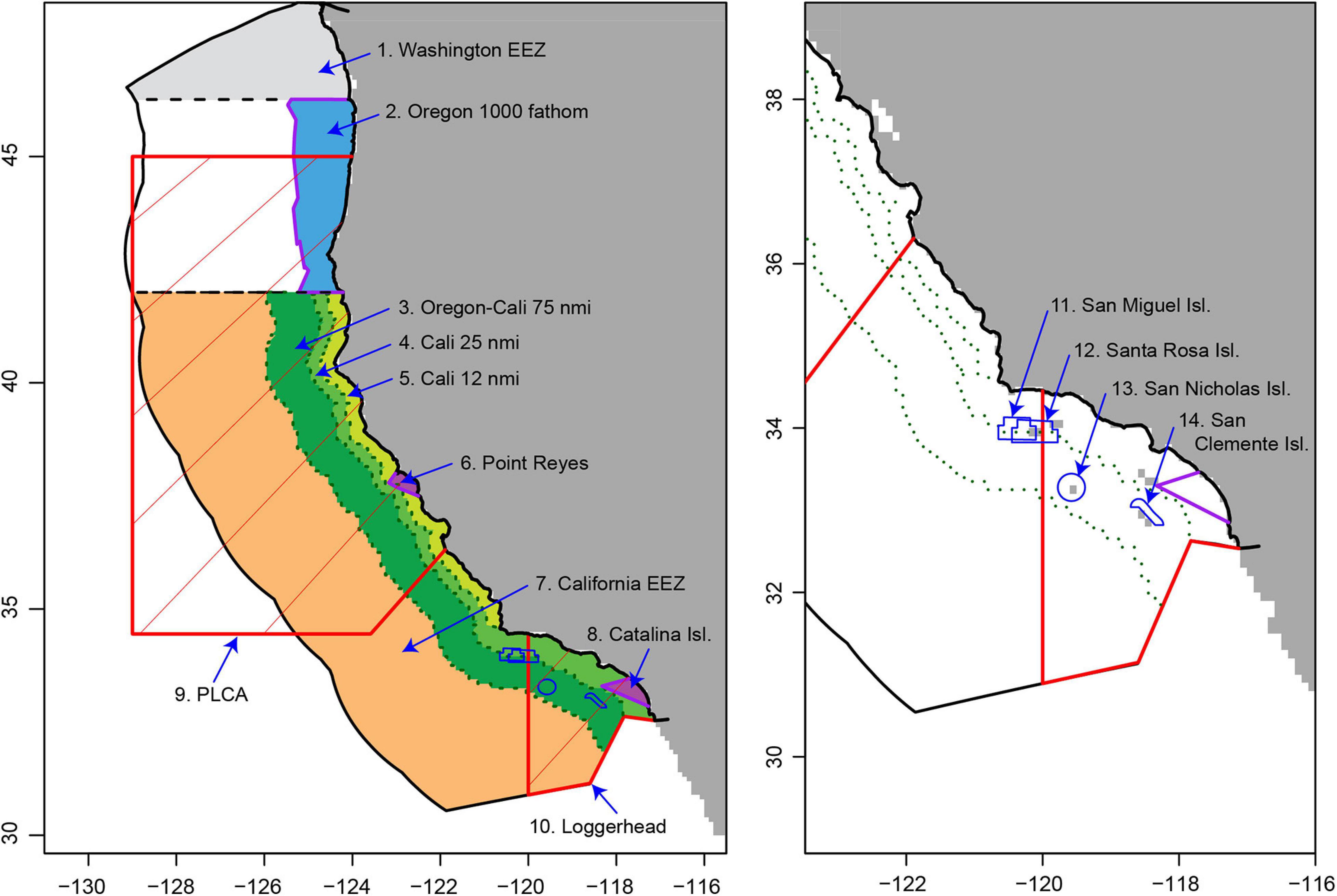
Figure 1. The closure areas implemented in the DGN and in our simulation (n = 12; see Supplementary Material S1 for closure dates), with the exception of the Pacific Leatherback Conservation Area (PLCA) and Loggerhead Conservation Area (red lines) which were not implemented in our simulation.

The goal of our study was to compare the performance of static and EcoCast-based dynamic time-area closures, aimed at reducing bycatch of two species, using a simulation based on the DGN. Of particular interest were: (1) quantifying the trade-off between bycatch avoidance and economic considerations such as target species catch and trip-level profit, (2) exploring sensitivity of closure performance to the dynamism of a species’ distribution and the size of an observer program, (3) quantifying the magnitude of variation in simulated catches due to interannual ocean variability, and to stochastic elements such as the location of fishing and bycatch observation, and (4) identifying more generally the conditions under which time-area closures and the subsequent redistribution of fishing effort are likely to be effective tools for bycatch mitigation.

Materials and Methods

General Simulation Approach

Our simulation used a management strategy evaluation (MSE) framework (Figure 2). MSE is a closed-loop simulation, comprised of one or more operating models representing the assumed ‘true’ biological and fishery conditions, and a management process representing the detection and response of management to the operating model (Punt et al., 2016). In our case, the operating models defined the ocean state, fishing locations, and the distribution of potential catch and bycatch, while the management process defined the observer program and the creation and implementation of static and dynamic time-area closures (Figure 2A). The MSE framework was particularly appropriate in this study, because leatherback turtles are rarely encountered in the DGN (Martin et al., 2015; Mason et al., 2019), which makes their distribution and bycatch risk challenging to quantify. By using MSE, we were able to characterize this uncertainty by testing multiple plausible operating models of leatherback distribution, and evaluate closure strategies assuming each operating model was true.

FIGURE 2

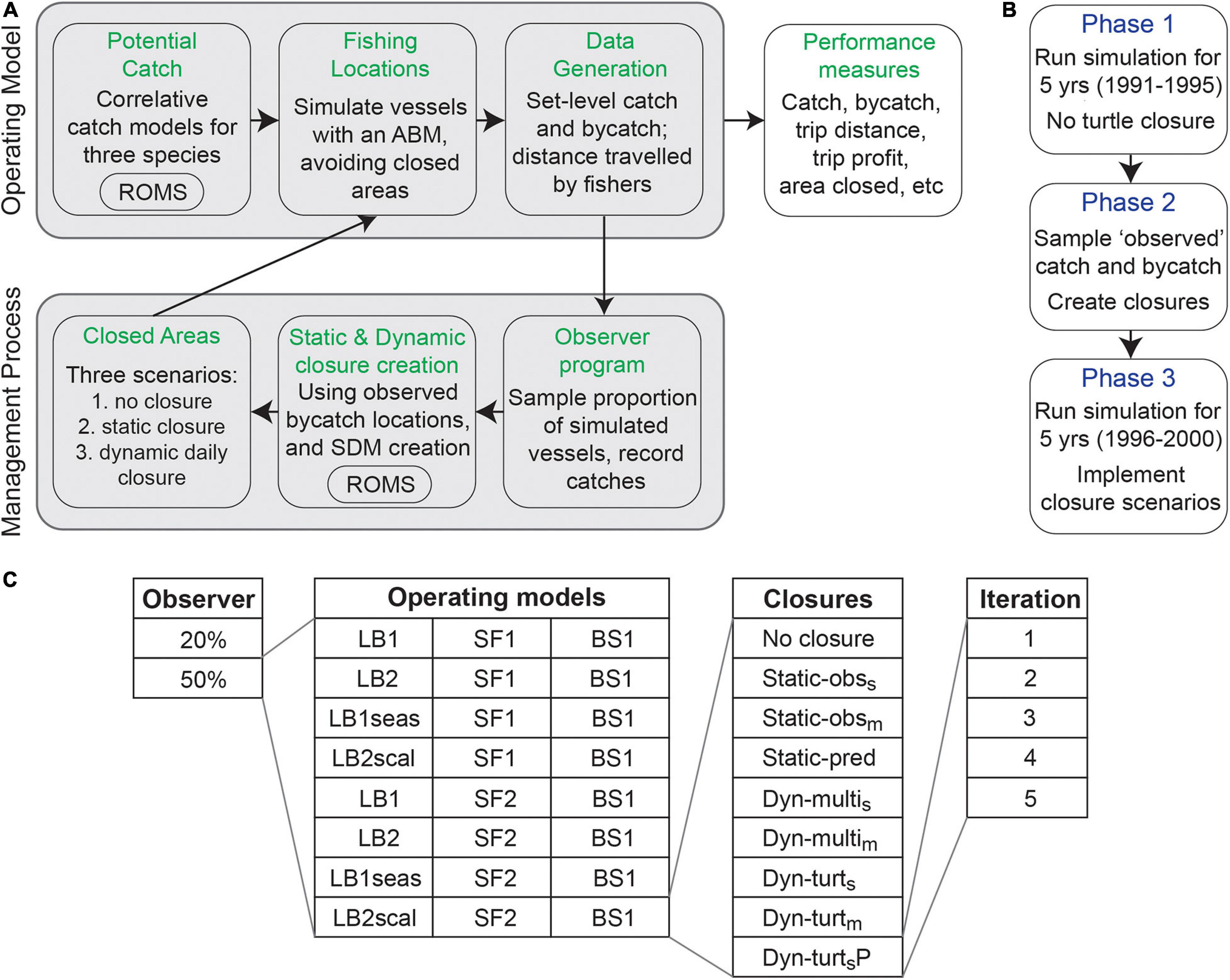
Figure 2. Our simulation framework, describing the MSE loop (A), the phases in which the simulation progressed (B), and the variations and closure strategies tested (C). The operating models were eight combinations of leatherback turtle (LB), swordfish (SF), and blue shark (BS) catch models, and are defined alongside the static and dynamic (Dyn.) closure strategies in Table 2. Output from a California Current System implementation of the Regional Ocean Modeling System (ROMS) informed the spatially explicit catch models for swordfish, blue shark, and leatherback turtles, as well as the species distribution models (SDMs) used to create the dynamic closures. The number of runs was 80 in Phase 1, and 720 in Phase 3.

Although our simulation closely represents the DGN, the simulated static and dynamic closures are dependent on the specific leatherback distribution scenario simulated in the operating model (‘simulated truth’) and thus do not represent actual closures in the DGN. Our simulation should be considered a hypothetical fishery because the simulated static closures, although created to represent a PLCA-like closure (Figure 1), differed from the PLCA in shape and location. Thus, our simulation does not attempt to identify the best closure for reducing leatherback turtle bycatch in the actual DGN; rather, we use the DGN as a guide for a realistic fishery in which to compare the relative performance of static and dynamic time-area closures, given uncertainties in the biological and management systems.

The Drift Gillnet Fishery

The DGN is a federally managed fishery which has operated over the period from 1980 to the present in the national waters of the U.S. west coast. It targets highly migratory species (HMS) with swordfish being the dominant targeted species (currently contributing ∼86% of total revenue; Pacific Fisheries Information Network, PacFIN). The DGN commonly catches non-target species such as blue sharks and molas (Mola mola), which are not marketable, and more rarely interacts with marine mammals and sea turtles (Mason et al., 2019). DGN vessels remain at sea for multiple days before landing their catch, and deploy the gillnet (as a ‘set’) typically overnight. The exclusive economic zone (EEZ) off California is closed annually to the DGN from 1st February to 30th April, and is closed from the coast to 75 nm from shore from 1st May to 14th August, meaning that a de facto DGN fishing season operates from 15th August to 31st January (Supplementary Material 1).

The DGN has a complex management history with numerous regulatory changes, and participation in the fishery has declined substantially over the last 20–30 years (Holts and Sosa-Nishizaki, 1998; Urbisci et al., 2016; Mason et al., 2019). A number of regulations have been implemented to reduce bycatch, including gear modifications and time-area closures. There are currently 14 permanent or temporary closures, including two time-area closures aimed at reducing bycatch of sea turtles (Figure 1 and Supplementary Material 1). The largest of these closures is the PLCA, which was designed to encompass the majority of observed leatherback turtle bycatch events. The PLCA was implemented in 2001 and is enacted each year from 15th August to 15th November. This closure timing is considered effective at reducing interactions with leatherback turtles (Eguchi et al., 2017). It is also considered to have contributed to a reduction in effort and landings of swordfish on the U.S. West Coast. Continued assessment of the economic impacts of these (and potential) regulations and closures is important to ensure thorough evaluation of the trade-off between bycatch reduction and economic opportunity; especially in the context of absolute bycatch impact (which for the DGN is comparatively low; Savoca et al., 2020), and considering the potential for “leakage” and “spillover” of the bycatch problem for many HMS (Chan and Pan, 2016; Helvey et al., 2017).

The National Marine Fisheries Service (NMFS) established a federal observer program for the DGN in 1990, usually covering 15–20% of fishing trips. This program provides a range of information, including the dates and locations of all sets and set-level counts of all caught species. We used this observer data to develop catch models for swordfish, blue shark, and leatherback turtles. We selected these two bycatch species due to the influence of leatherbacks on the DGN’s current spatial management, because both leatherbacks and blue sharks are included in EcoCast, and because blue sharks represent a commonly encountered species to contrast the rare bycatch of leatherbacks. The DGN also uses logbooks that report total landings, and these data were used to determine realistic total fishing effort in our simulation. A cost-earnings survey has also been done for this fishery (years 2009–2010; NMFS, unpublished data), which provided essential information on variable fishing costs (Smith et al., 2020).

The MSE Simulation

Simulation Framework

The simulation framework consists of an MSE simulation loop (Figure 2A), which was run in three phases (Figure 2B), and repeated numerous times to include a range of operating models (uncertainty scenarios) and spatial management strategies (Figure 2C). The operating model in the MSE loop defined the distribution and catch rate of swordfish, leatherback turtles, and blue sharks. These were correlative catch models informed by a suite of habitat variables, including dynamic ocean covariates taken from a data-assimilative implementation of ROMS configured for the California Current (Neveu et al., 2016)¹. The MSE operated at the scale of the ROMS output: daily, and at a 0.1° (∼10 km) horizontal resolution. We simulated eight operating models, corresponding to eight combinations of our catch models, to incorporate uncertainty in the distribution of leatherback turtles and swordfish. The catch models were used to predict daily potential catch across the entire domain, given each day’s environmental conditions, with set-level catches determined by simulating a fishing process using an agent-based model (ABM) which did not allow fishing in closed areas.

Closed areas were determined by the simulated leatherback closure defined by the spatial management strategy being assessed. We evaluated performance of nine spatial management strategies, which were a no closure reference strategy, three static closures, and five dynamic closures. Each operating model and management strategy combination was iterated five times to incorporate random variation in which trips were observed, model-based closure creation, and fishing locations and simulated catch (Figure 2C). We also repeated the entire simulation for two levels of an observer program (20 or 50% coverage of vessels) to explore how the amount of bycatch information influenced closure performance. Given how our model was tuned, 20% coverage represented a minimum amount to create our dynamic closures, and we chose to explore whether increasing information above this minimum improved closure performance (and not because we are specifically interested in 50% coverage). Of interest, but beyond the scope of our study, would be to explore the relationship between observer coverage, bycatch rate, and SDM performance. This would be important when evaluating the suitability of dynamic closures in real-world fisheries with less observer coverage. Catch and fishing information (e.g., distance traveled, profit) were recorded and stored for evaluation of closure performance.

In Phase 1 of the simulation, the MSE loop was run for 5 years without a leatherback closure. This created 5 years of an observer program with which to create leatherback closures. In Phase 2 (which occurred instantaneously), the data from this observer program (given either 20 or 50% coverage of trips; Figure 2C) were used in the creation of static and dynamic time-area closures to be implemented in Phase 3. In Phase 3, the MSE loop was run for another 5 years, this time with a leatherback closure implemented. The performance metrics recorded in Phase 3 were those used to compare performance of the various closure strategies, often with respect to the baseline ‘no closure’ strategy (Table 1). The simulation was developed in R (v3.6.3; R Core Team, 2020).

TABLE 1

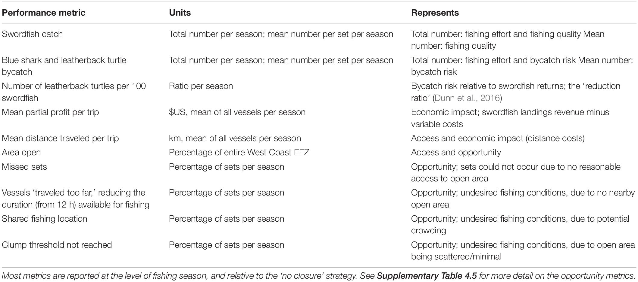
Table 1. Summary of the key performance metrics used to evaluate closure strategies.

Catch Models

The distribution of potential catch for the three species was determined using correlative SDMs (Figure 3). These were fitted to the actual observer data for the DGN, from 1990 to 2000 (∼5700 observed sets). This period was selected as it was before the implementation of the PLCA closure, and thus before the distribution of fishing effort changed considerably. We created four leatherback turtle catch models and two swordfish models to define the distribution of potential catch and bycatch (Table 2). Varying the leatherback model allowed us to explore closure performance across plausible differences in leatherback distribution (LB1 and LB2), as well as explore the impact of species distribution type (seasonal or broad) on closure performance (LB1seas, LB2scal). It was important to test plausible differences in swordfish distribution (SF1, SF2), because the distribution of expected and recent swordfish catch influenced fishing locations (see the ABM below). Only a single blue shark catch model was used, in order to keep the number of operating models manageable.

FIGURE 3

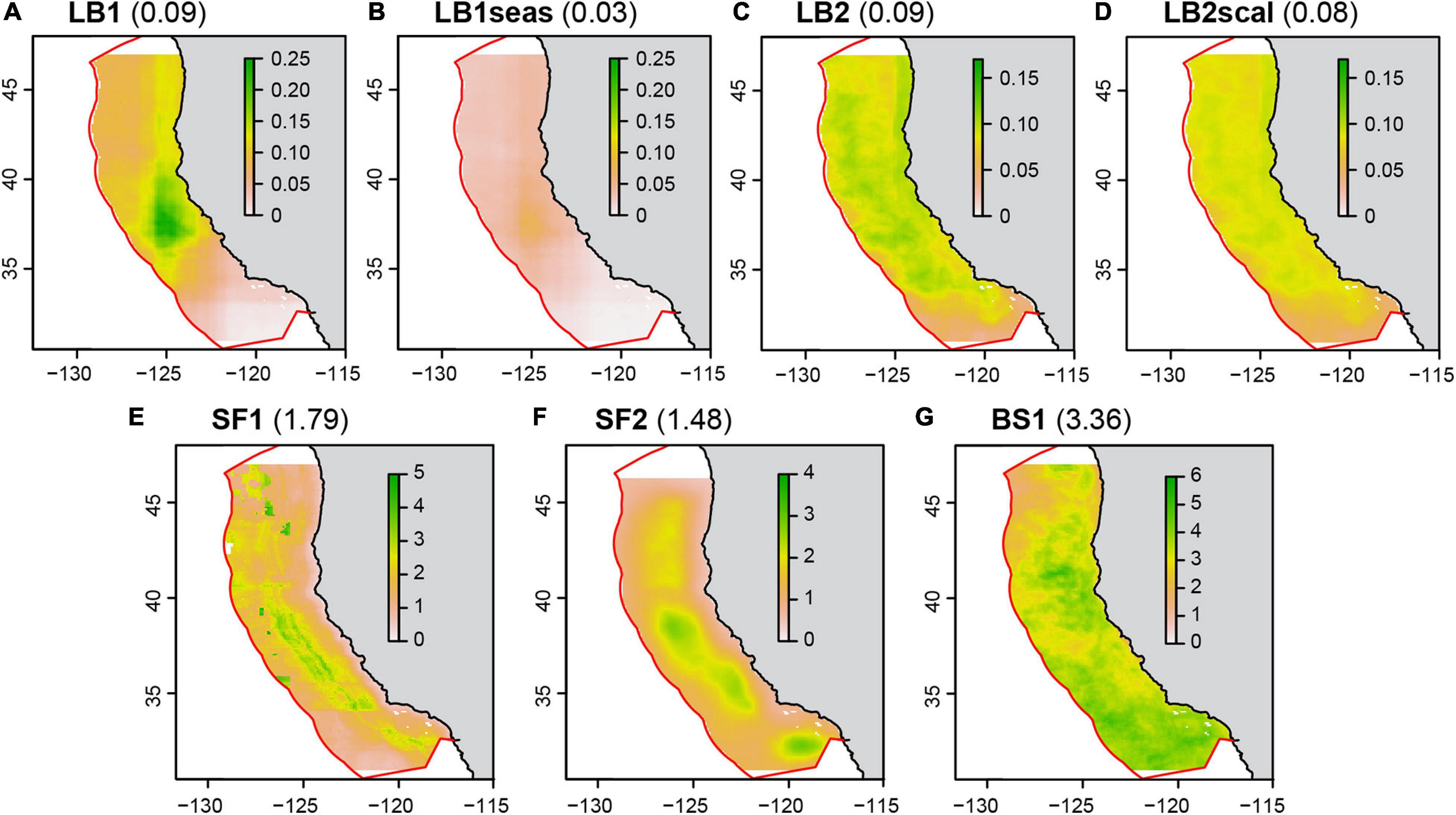
Figure 3. Predicted catch by the seven catch models used to define the operating models (Table 2). Shown is the mean predicted catch for November (i.e., the mean of all November days for 1991–2000; the mean November catch rate averaged across the domain is in parentheses); November was chosen as this has high fishing effort. The color is the predicted mean probability of catching one leatherback per 12 h set (A–D), or the mean number of swordfish (E–F) or blue sharks (G) per 12 h set. See Supplementary Material S2 for example maps of daily predicted catch. The latitudinal limits of prediction were due to the limits of the FTLE variable, except the northward limit in SF2 which was the limit of the soap film smoother.

TABLE 2

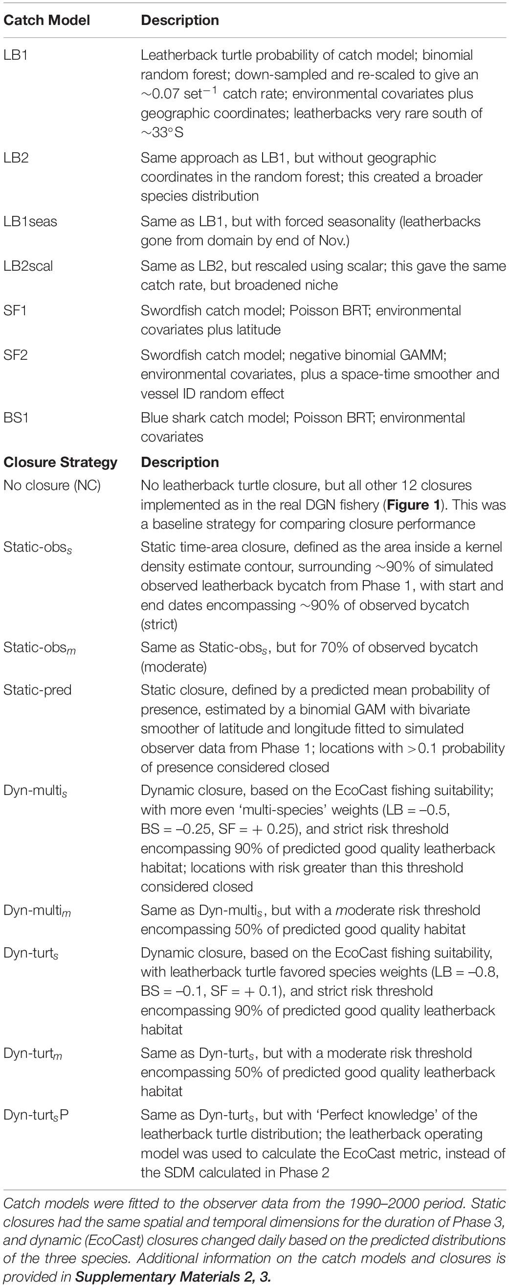
Table 2. Summary of the seven catch models used to define the operating models, and the nine static or dynamic closure strategies.

A variety of correlative models were used to develop the catch models (Table 2 and Supplementary Material 2). Classification trees (random forests; Breiman, 2001) were used to model leatherback bycatch due to the very low number of observed bycatch events (n = 23), and random forests are known to be robust for modeling rare bycatch (Carretta, 2018; Stock et al., 2019). Given that a maximum of one leatherback turtle is typically caught per DGN set, we chose to model leatherback catch rate as a Bernoulli process (catch of zero leatherbacks or one leatherback). Predicted probabilities for classification trees were then defined as the proportion of votes of each class from the individual trees. We used down-sampling to correct imbalance in the absence and presence classes of observation (Stock et al., 2019). Like other authors (Stock et al., 2018), we found that class imbalance-corrected random forests overpredicted bycatch rates, and we rescaled the predicted bycatch probabilities using a general updating approach (Elkan, 2001; Suppementary Material 2). However, our simulation was designed so that leatherback closures could be created using a simulated observer program, and the actual observed bycatch rate (∼0.004 per set) was too low to create useful closures over a short period (especially the SDM-based dynamic closures). In practice, EcoCast incorporates animal tracking data to create risk surfaces for rare species (Hazen et al., 2018), but tracking data were too complex to simulate in our MSE (which would require not only a simulated observer program but also simulated animal locations and a tracking program). Thus, we rescaled the leatherback bycatch probabilities to have an inflated bycatch rate of ∼0.07 leatherbacks per set for each catch model. Testing showed this catch rate was near the minimum required to create the dynamic closures without fitting issues (given 20% observer coverage). Thus, the absolute bycatch rate in our study does not represent that in the actual DGN, but closure comparisons using percent bycatch reduction are indicative of performance given rare bycatch species with a leatherback-like distribution.

There were two main random forests fitted for leatherback turtle catches (LB1 and LB2; Table 2). While both generated plausible bycatch distributions relative to observed bycatch events (Supplementary Table 2.2), they were reflective of different potential leatherback distribution patterns. Both models included environmental covariates and an effort covariate (set duration), but only one also included geographic coordinates (LB1). LB1 represents a leatherback distribution with core habitat off central California (Figure 3), which agrees with existing research indicating this may be part of, and a transit region for, an important foraging area (Eguchi et al., 2017). LB2 represents a broader and more variable leatherback distribution which is determined predominantly by dynamic habitat variables (Supplementary Material 2). The LB1seas model is identical to the LB1 model, but with a forced migration signal that removes leatherbacks from the domain by the end of November. This was done to match telemetry patterns (Benson et al., 2011), and to represent a leatherback distribution potentially more amenable to spatial management (i.e., bycatch risk exists in a smaller and more predictable part of the fishing season). The LBscal model was rescaled using a fixed scalar, which created a leatherback distribution with the same mean catch rate but less difference between ‘high bycatch risk’ and ‘low bycatch risk’ habitat (Suppementary Material 2). This represents a distribution potentially less suitable for spatial management (i.e., redistributing vessels from high risk to low risk areas will have less impact on bycatch reduction). More information on model covariates, rescaling, performance, and fitted parameters are provided in Supplementary Material 2.

The two swordfish catch models (SF1 and SF2, Table 2) were fitted to the observer data as a boosted regression tree (BRT; SF1) or generalized additive mixed model (GAMM; SF2). GAMMs and BRTs are common tools for species distribution modeling; both have shown success in modeling the distribution of potential swordfish catch (Smith et al., 2020) and both were plausible models based on their similar predictive performance (Supplementary Table 2.3). The GAMM included environmental covariates, a space-time tensor using a soap-film smoother for geographic coordinates, and a vessel ID random effect (using bs = “re”). The BRT included environmental covariates and latitude. Both models included the effort covariate (set duration). Swordfish catch (number per set) was modeled with a negative binomial family in the GAMMs and a Poisson family in the BRT (36% of sets caught zero swordfish). Evaluation of residuals and overdispersion in the GAMM showed the negative binomial was appropriate. This family was not available for the BRT, but an evaluation of the model prediction from the BRT showed a sensible distribution of catch rates (evaluated in Smith et al., 2020). The blue shark model (BS1, Table 2) was fitted as per SF1, using a Poisson BRT. More information on these models is provided in Supplementary Material 2.

These seven catch models were used to predict potential catch across the modeled domain (Figure 3) for each day of the simulation, and saved as rasters for use in the MSE loop. The prediction specified set duration at 12 h, which was the mode and median from the observer data. Predicted potential catch was thus the mean number of swordfish or blue shark per 12 h set, or the mean probability of catching one leatherback turtle per 12 h set. By modeling catch statistically and without population dynamics, our study evaluated closure performance under assumptions of fixed population abundance and no depletion at any spatial scale.

Spatial Management Strategies

Our MSE compared nine time-area closure strategies (Table 2). Each static closure kept the same spatial and temporal dimensions for the entire Phase 3 (Figure 2B) but these dimensions changed between operating models and iterations. Dynamic closures changed daily, and also changed between operating models and iterations, and were implemented for the entire fishing season. The reference closure strategy was ‘no leatherback closure,’ in which there was no closure and vessels were free to fish anywhere outside other closures (Figure 1).

We simulated three static closure strategies (Table 2). These were based loosely on the PLCA, which was designed to enclose the majority of observed leatherback turtle bycatch (Figure 1). We used two methods to approximate this design process in our simulation: kernel density estimation and regression. Closure creation occurred in the management process (Figure 2A) in Phase 2 of the MSE (Figure 2B) using the simulated observer data collected in Phase 1. The first approach created a kernel density estimate (KDE) of the simulated observed leatherback bycatch, and defined the closure as a threshold of that KDE. We term this the ‘Static-obs’ closure, to indicate a static closure that encompasses only observed bycatch events. We specified two thresholds: 70 and 90%, meaning that the KDE area (i.e., the closure) enclosed 70 or 90% of observed bycatch events. These thresholds correspond to the ‘Static-obs_m’ (moderate) and ‘Static-obs_s’ (strict) strategies (Table 2). The second approach used regression to create the closure, specifically a binomial GAM relating bycatch occurrence to a bivariate smoother of latitude and longitude; i.e., the probability of bycatch as a static function of location. A threshold probability was specified (0.1 probability of presence), and locations with bycatch probabilities higher than this threshold were considered closed. The key difference between the KDE and GAM approaches is that the KDE does not account for catch rate and is more influenced by the distribution of fishing effort, whereas the GAM models catch rate and may close areas that have a high bycatch rate relative to effort, even if the number of observed bycatch events is small. We thus term this closure ‘Static-pred’ to indicate the closure encompasses areas of predicted bycatch events. The PLCA is enacted for only part of the fishing season, with fixed start and end dates (Supplementary Material 1), so we also simulated start and end dates for the simulated static closures. As for the spatial extent, start and end dates were selected to encompass 70 or 90% of observed events (for the Static-obs closures) and 80% for Static-pred. For simplicity, start and end dates were evaluated at the monthly level, with closures starting or ending on the 15th of a month. Threshold values were arbitrary, but were selected so that the amount of fishable area closed was comparable to the PLCA and relatively similar among strategies. Examples of the static closures are shown in Figure 4.

FIGURE 4

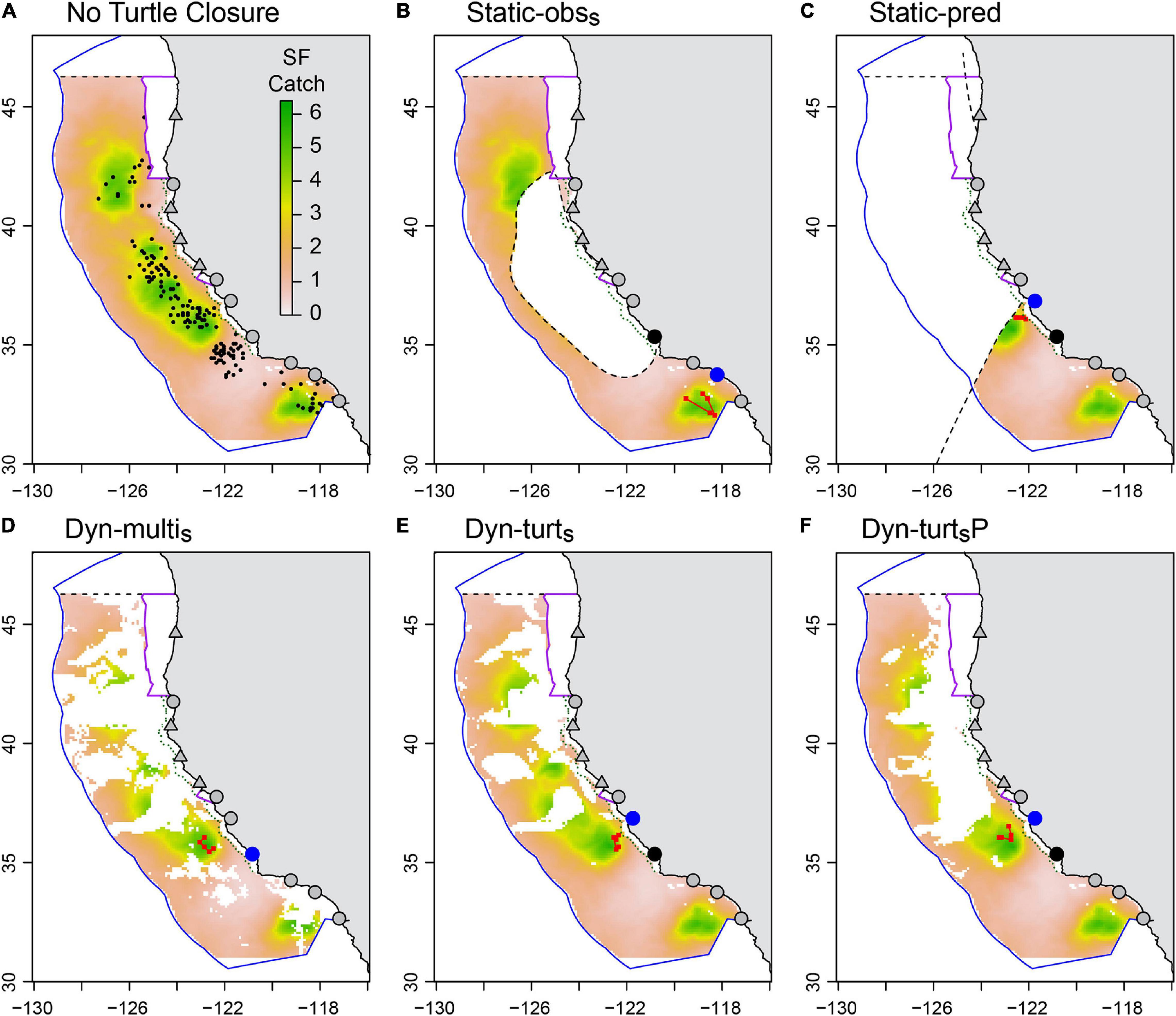
Figure 4. Maps of closure strategies for an example date (2nd November 1997), with color indicating the potential swordfish catch (number per 12 h set) defined by model SF2. White areas indicate closures (or area outside the EEZ). Also shown are six ports used as departure ports in our simulation (gray circles), plus four ports available for landing only (gray triangles). Panel (A) shows the non-turtle closures active on this date (Washington, Oregon 1000 fathom, California 12 nm, Point Reyes), and the simulated observed leatherback turtle bycatch events (black dots) for an iteration of Phase 3 of the LB1-SF2 operating model for the no closure strategy. Panels (B,C) show the additional closed area on this date due to the Static-obs_s (B) and Static-pred (C) closures (dashed black lines are closure borders). In this iteration, these closures were implemented from 15-July to 15-December (Static-obs_s) and 15-August to 15-December (Static-pred). Panels (D,E) show the additional closed area due to the strict dynamic closures, with EcoCast evenly weighted (D) or turtle weighted (E). Panel (F) shows the closed area if the Dyn-turt_s closure had perfect information on the distribution of potential leatherback bycatch. Also illustrated in panels (B–F) are example fishing trips simulated by our ABM. These vessels departed Morro Bay (black circle), made five sets (red squares) then landed their catch at the nearest port (blue circle).

We simulated five dynamic closures (‘Dyn’; Table 2), all created using the EcoCast decision support tool (Hazen et al., 2018). EcoCast sums predictions from presence-absence SDMs of multiple species to generate a fishing suitability (or risk) surface, with weightings used to determine each species’ contribution to the calculated risk. EcoCast can include both bycatch and target species and weight each more negatively (for bycatch species) or positively (for target species) depending on the prioritization of species. Our closures were defined as those areas with predicted bycatch risk greater than a specified threshold. We specified a three-species EcoCast (swordfish, leatherback turtle, blue shark) to explore one key aspect of EcoCast – the ability to balance objectives for target and bycatch species – and to more closely resemble the multi-species version currently available to DGN fishers (Hazen et al., 2018; Welch et al., 2020). EcoCast risk surfaces were created in Phase 2, by: (i) creating environmentally informed SDMs for each species using the simulated observer data matched to environmental data from ROMS; (ii) predicting the risk surface for every day in Phase 3; and (iii) closing to fishing for every day in Phase 3 the areas with EcoCast values above the risk threshold. The SDMs were created using BRTs in an approach very similar to that used for EcoCast. The four EcoCast closure strategies were strict and moderate thresholds for two species-weighting scenarios (Table 2). The species weightings represent a ‘multi-species’ closure in which the habitats of all three species were evenly weighted (‘Dyn-multi’; i.e., habitats with high leatherback bycatch risk will have their risk reduced if they are also good swordfish habitat and/or poor blue shark habitat), and a ‘single-species’ closure in which leatherbacks were prioritized over the other species (‘Dyn-turt’; i.e., habitats with high leatherback bycatch risk will remain high risk regardless of suitability for the other species). The EcoCast thresholds were calculated using an iterative process to encompass 90% (strict) or 50% (moderate) of the ‘good quality’ leatherback turtle habitat (defined as > 0.1 probability of occurrence). Thus, ‘Dyn-turt_s’ represents the closure with the highest leatherback avoidance objective. These threshold values were selected so that the amount of fishable area closed was comparable between static and dynamic closures.

An important element of MSE is ensuring that the information from the operating model available to the management process has realistic error (Punt et al., 2016). In our case, it was key to ensure that the SDMs used to calculate EcoCast and create the dynamic closures were realistically accurate, given that SDMs were also used to define the operating models. We did this by simulating an observer program, and by using structurally different models for the operating model and EcoCast closure SDMs. We evaluated accuracy, and found that EcoCast had a similar predictive power in the simulation (AUC = 0.66–0.81) as it does in the real world for leatherback turtles (AUC = 0.77; Welch et al., 2020), so no additional error was simulated. The final ‘Dyn-turt_sP’ strategy was created, in part, to explore this simulated and real-world accuracy (Table 2), and performance of this closure represents maximum EcoCast performance given perfect knowledge (no observation or estimation error) of the distribution of leatherback turtles. More information about EcoCast fitting, thresholds, and validation is presented in Supplementary Material 3. Examples of the static closures are shown in Figure 4.

Fishing Effort and Agent-Based Model

Our MSE used an agent-based model (ABM) to simulate fishing (Figure 2). It was essential to have a dynamic tool like an ABM so that the fishing locations responded realistically to fishing closures (especially the daily updated dynamic closures). The ABM simulated individual vessels and their fishing effort, movement, and catches, and was based on a profit maximization framework, whereby agents (i.e., fishing vessels) make decisions that maximize their utility (van Putten et al., 2012). Here, utility was measured as a vessel’s expected partial profit, which is the revenue from expected swordfish catch minus fuel and crew costs. Because DGN vessels fish for multiple days, with presumably an expectation of trip duration, we calculated trip-dependent utility. This estimates the utility of a location if it was fished on a trip of specified duration and expected distance traveled (Smith et al., 2020). Our ABM operated in two stages: (1) utility was calculated for all cells in the fishable domain; and (2) the cell with the highest expected utility was selected from all accessible and available cells (i.e., those that can be traveled to within a specified time and are not in an active closure) using an accuracy term representing an agent’s imperfect detection of utility. The ABM is further detailed in Supplementary Material 4. See Figure 4 for example vessel tracks.

Fishing effort was determined by the number of sets each day and their duration. Set duration was fixed (12 h) for tractability as well as computational efficiency (set duration was a covariate in the catch models, and the predicted daily catch rasters were created outside the MSE loop). The number of vessels and sets to simulate in the ABM was estimated from DGN logbooks (sourced from PacFIN). We calculated logbook mean monthly effort and allocated this to 5-day fishing trips, which were then distributed to key departure ports based on the recorded departure ports in the observer data (1990–2000). This resulted in a monthly number of sets that matched the logbook effort, while closely matching the observed proportional use of specific departure ports. The departure dates of fishing trips within each month were allocated randomly, so that for each iteration of the simulation the daily fishing effort could vary (even if the mean monthly effort could not). We fixed the duration of every fishing trip at five overnight sets (the median value from the observer data) for tractability.

Our ABM operated at the set level, so catches needed to be integers (i.e., number per set). Thus, we calculated catch of each species as a random sample from the distribution of each catch model (negative binomial or Poisson for swordfish, Poisson for blue sharks, binomial for leatherbacks) given the mean catch rate predicted by each catch model (and fitted dispersion parameter for the negative binomial). An advantage of this approach was the realistic variation in catches among sets and vessels, and we found close agreement between simulated and observed catch frequencies (Supplementary Figure 5.2). There were numerous parameters used in the ABM that influenced fisher behavior, such as swordfish price and initial step distances (Supplementary Material 4), but these were not varied in our simulation in order to keep the number of iterations manageable. Thus, our results represent closure performance given ‘mean’ vessel behavior, and changes to aspects such as vessel mobility could have considerable influence on closure performance, e.g., near-shore time-area closures may have a greater economic impact on lower mobility vessels (Smith et al., 2020).

Performance Metrics

The metrics we used to evaluate closure performance are summarized in Table 1. They were focused on the total coast-wide catch and bycatch of the three species per fishing season, as well as the mean catch and bycatch rate (per set). We also measured closure performance using profit, distance traveled, and fishing opportunity. Fisher profit and distance traveled were measured at the trip level. Fishing opportunity was measured at the set level, and was represented by the number of missed sets, the frequency of shared fishing cells, and the frequency of undesirable travel behavior (see Supplementary Table 4.5). Unlike more tactical MSEs, ours did not have specific management objectives or targets, except that a successful closure would reduce leatherback turtle bycatch (compared to no closure), and beyond that provide balance in other economic and bycatch metrics (e.g., target swordfish catch, profit, area open, blue shark bycatch).

Simulation Validation and Uncertainty

We compared various simulation outputs with observations to ensure our simulation was representative of DGN dynamics and thus a useful comparison of static and dynamic closures. Reasonable accuracy was important for the ABM in which numerous parameters were tuned to create realistic agents. We compared total simulated swordfish landings and their variation throughout the fishing season against observations. To help tune the ABM, we compared observed and modeled data for: swordfish per-set catch rates; the distance offshore of fishing locations; the travel distance between sets; and the general spatial distribution of fishing effort (Supplementary Material 5). In general, we found close agreement between simulated and real-world fishing, although we could not reproduce the same level of near-shore fishing (Supplementary Figure 5.3). The broader distribution of fishing was accurate (Supplementary Figure 5.5).

A key element of MSE is incorporating all relevant uncertainties (Punt et al., 2016). Our simulation focused on incorporating uncertainty in: the distribution and catch rates of swordfish and leatherback turtles; choice of fishing location; SDM construction; the fine-scale timing of fishing effort; and which trips were observed. These and additional sources of uncertainty are detailed in Table 3. We were able to allocate general sources of variation (environmental, closure creation, other; Table 3) in our simulation, by comparing differences in key outputs among bootstrapped pair-wise comparisons of simulation runs. This method is detailed in Supplementary Material 5.

TABLE 3

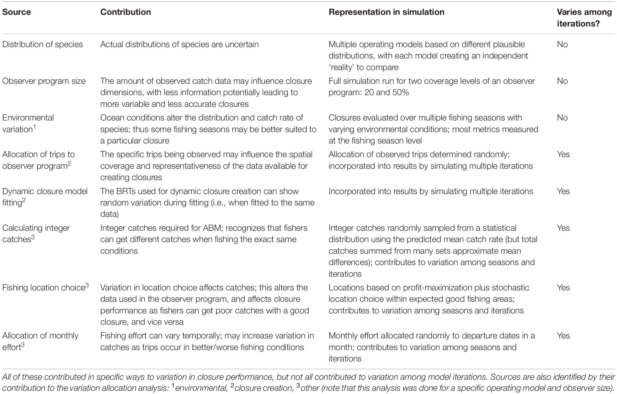
Table 3. Summary of the sources of uncertainty and variation in our simulation.

Results

Closure Performance

In terms of swordfish catch, the strict Static-obs_s closure clearly performed worst, leading to 25–40% fewer swordfish per season compared to no turtle closure (Figure 5A). Trip profit showed the same pattern as swordfish (Supplementary Figures 6.2–6.5), showing that lost revenue was the predominant economic driver, as opposed to additional distance costs. For both LB1 and LB2, this decline in swordfish catch was due to reduced access to good quality swordfish habitat (see ‘swordfish per set’ results, Supplementary Figure 6.2), and for LB2 was also due to the Static-obs_s closure reducing fishing effort. Static-obs_s under the LB2 leatherback distribution reduced effort by 10–30% (Figure 5E). These boxplots indicate the considerable variation among fishing seasons and iterations for all performance metrics (Figure 5).

FIGURE 5

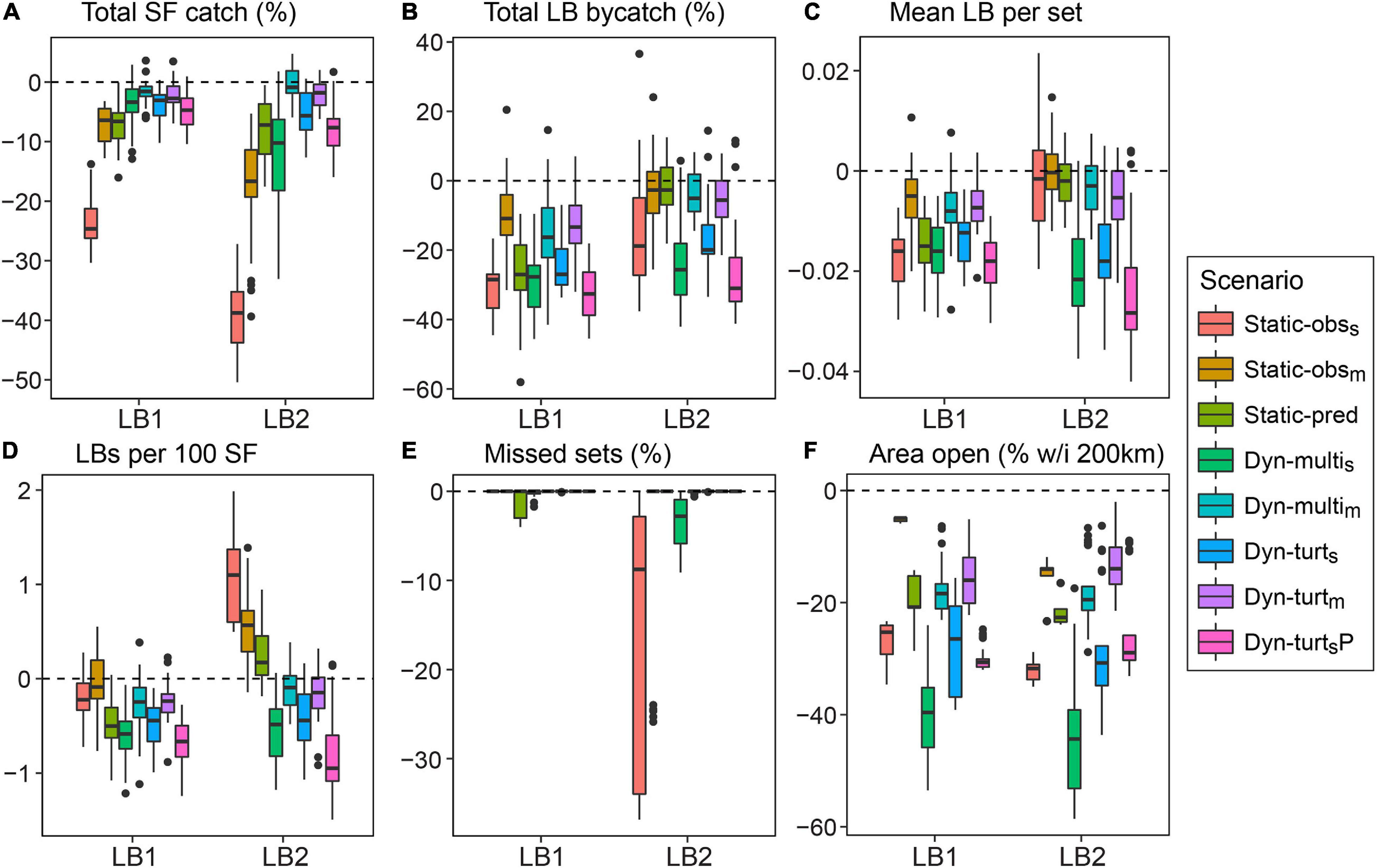
Figure 5. Boxplots summarizing differences between closure strategies for six key performance metrics. This compares results from the LB1 and LB2 models, using the SF1 model and 20% observer coverage (see Supplementary Material S6 for the other operating models). All reported values are per season and represent differences from the ‘no turtle closure’ strategy; e.g., compared to no turtle closure, having the Static-obs_s closure meant 25–40% fewer swordfish caught per season. Each boxplot contains five iterations of five seasons (n = 25). Units in panels (A,B,E) are percentage changes, (C,D) are absolute catch rates, and (F) is the absolute area (as a % of total area within 200 km from shore).

The moderate closures (Static-obs_m, Dyn-multi_m, Dyn-turt_m) produced the smallest reduction in leatherback turtle bycatch, showing that closures can be largely ineffective if only some habitat is protected and fishing effort is mostly redistributed (Figure 5B). Static-obs_s and Static-pred achieved bycatch reduction under the more static LB1 leatherback distribution, but were largely ineffective when the leatherback distribution was broader and more dynamic (LB2). Leatherback bycatch per set indicates whether fishing effort was redistributed into less risky habitat. According to this metric, both static and dynamic closures were effective under the LB1 model, but only the strict dynamic closures were effective under LB2 (Figure 5C). Thus, the decline in total bycatch by Static-obs_s under LB2 was due to reduction in fishing effort, not the effective redistribution of fishing effort to less risky areas. In terms of balancing bycatch and target catch, the ‘turtle per swordfish’ metric showed that strict dynamic closures were most effective, and Static-obs_s the worst (Figure 5D). The absolute means under the no closure strategy were 2.3 leatherbacks per 100 swordfish for LB1 and 3.5 for LB2.

Both Static-obs_s and Dyn-multi_s reduced blue shark bycatch by 20–25% under the LB2 model (Supplementary Figure 6.3), in which closures were often larger and extended into Southern California. However, this reduction was less than the reduction in swordfish catch. Other closures had negligible impact on blue shark bycatch, most likely due to this species’ very broad simulated distribution (Figure 3).

In terms of fishing opportunity, all closure strategies closed 40–80% of the fishable area (i.e., waters within 200 km from shore), with 15–45% more area closed than with no turtle closure (Figure 5F). The Dyn-multi_s closure closed the most area (Supplementary Figure 6.6 and Supplementary Table 6.1) because the EcoCast threshold needed to be stricter in order to protect 90% of good quality leatherback habitat given the additional constraint of considering the other species’ distributions. Even so, most fishing could still occur in open fragments of habitat, and the distribution of fishing effort under dynamic closures was similar to that with no closure (Figure 6). For dynamic closures, the area open was similar among fishing seasons except for 1997, which was an anomalous year with low predicted bycatch risk (Supplementary Figure 6.6). The area open within a season for dynamic closures was more variable for the LB2 model. Although the Static-obs_s closure had the most impact on fishing effort (Figure 5E), the dynamic closures more often induced undesirable fishing conditions, such as location sharing or traveling too far, but these occurred in <5% of sets (Supplementary Figure 6.1).

FIGURE 6

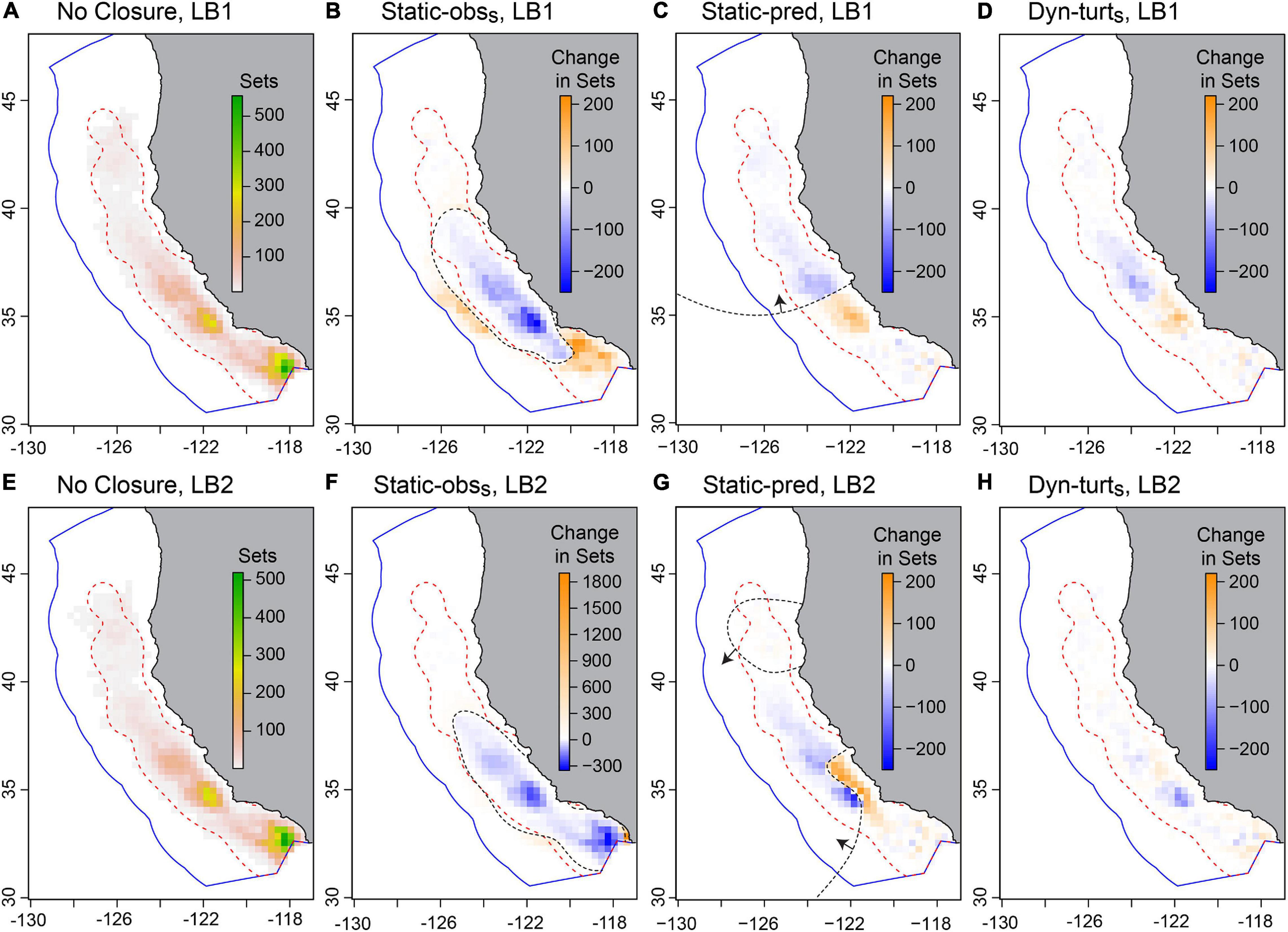
Figure 6. The distribution of simulated fishing effort under no closure (A,E), and the change in this effort under strict static closures (B,C,F,G) and the strict turtle-weighted dynamic closure (D,H), for the LB1 and LB2 leatherback models. These represent one iteration and using the SF1 model. In (A,E) color indicates effort, which is the total number of sets per 0.3°-degree cells during Phase 3 (i.e., five fishing seasons and ∼15,000 sets); in other panels color indicates the change in the number of sets (blue indicates a decrease, and orange an increase, in fishing effort compared to no closure). The red dashed line contains 95% of real-world observed effort and the dashed black line is the boundary of the static closure for that iteration (arrows indicate direction of closed area for the Static-pred closure). For the Static-obs_s closure under LB2 (F) considerable effort was relocated into a single coastal cell (∼900 km²) at the very bottom of the domain. The distribution of actual effort (not the change in effort) is illustrated in Supplementary Figure 6.7.

We summarize closure performance across the two main leatherback models in Figure 7. In this study, we consider a successful closure one that reduces leatherback turtle bycatch without unreasonably impacting fishing effort and opportunity. Thus, the Static-pred closure was the most successful static closure, but it was only effective under LB1. Dyn-turt_s or Dyn-multi_s could be considered the most successful dynamic closures, and were the only closures to effectively reduce leatherback bycatch under LB2 (Figure 7). As expected, having perfect information for the distribution of leatherbacks (Dyn-turt_sP) improved closure effectiveness, providing an additional 6–15% bycatch reduction over Dyn-turt_s (Figure 5 and Supplementary Material 6).

FIGURE 7

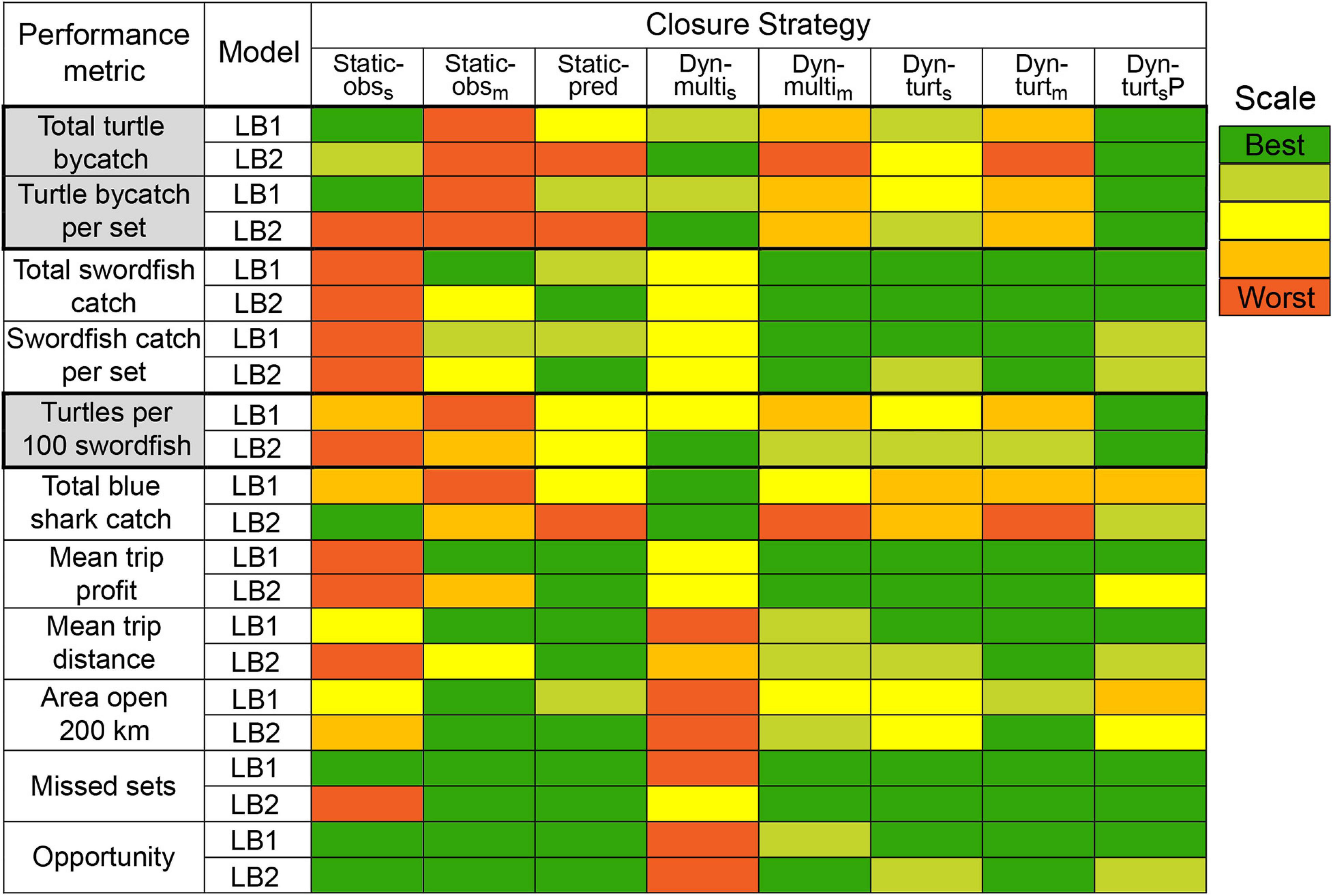
Figure 7. A summary of comparative median closure performance across performance metrics, for the two main leatherback models (LB1 and LB2). Color indicates whether a strategy had best (green) or worst (red) performance across the eight strategies, with additional colors indicating intermediate performance. Intermediate performance was calculated by dividing the range (max – min) of median values for each metric into five intervals and determining in which interval the median for each strategy was located. Thus, colors accurately represent relative performance within metrics but are arbitrary with respect to absolute performance, i.e., ‘best’ does not necessarily mean good performance (refer to Figure 5 and corresponding figures in Supplementary Material S6 for absolute values). This table summarizes across swordfish models, observer levels, and simulation iterations. The primary objective of simulated closures was reduction of leatherback turtle bycatch, and the relevant metrics are highlighted gray.

Additional Models, and Observer Size

Our simulation also compared closure performance across the two additional leatherback models (LB1seas, LB2scal), the two swordfish models, and the two observer program sizes (Supplementary Figures 6.8, 6.9). Performance was very similar between LB1 and LB1seas. We created LB1seas to represent a distribution of leatherbacks better suited to time-area closures, but because our simulation used the same closure thresholds for all simulation runs, closures in LB1seas simply ended earlier (and closed less area over the entire season Supplementary Figure 6.8 and Supplementary Table 6.1) while achieving the same bycatch reduction. To demonstrate how time-area closures may achieve better bycatch reduction for LB1seas, a stricter closure threshold would be required during the period the leatherbacks were present. We created LB2scal to represent a distribution of leatherbacks poorly suited for spatial management. This was clearly observed, with bycatch reduction for LB2scal only 50% of that for LB2 (compare leatherback catch per set in Supplementary Figures 6.3, 6.5, 6.8).

Closure performance occasionally differed between the two swordfish models. The swordfish models influenced the distribution of fishing effort, which differed more among fishing seasons for the SF2 model (due to the space-time smoother). The result was more variation in performance metrics for SF2 (Supplementary Figures 6.2, 6.3) and altered performance of some closures, e.g., Dyn-multi_s closed more area and reduced swordfish catch more under SF2 (Supplementary Figure 6.8). This highlights the considerable influence the distribution of fishing can have on closure effectiveness (i.e., how much fishing is redistributed and to where), and some of the complexities of multi-species closures (e.g., the degree of overlap among species will be highly influential).

Increasing the coverage of the observer program from 20 to 50% had little impact on closure performance (Supplementary Figure 6.9). This was especially true for LB1, indicating that a more static species distribution requires fewer observations to model accurately. Under LB2 and LB2scal, more observer coverage led to slightly better performance for strict static and dynamic closures, but this improvement was small, at 3–9% additional bycatch reduction over no turtle closure. We note that this improvement would be case-specific, and depend on the abundance of the species and the model being fitted, but for our study (and somewhat by design) 20% coverage provided acceptably accurate models of species’ distributions (20% coverage corresponded to 160–240 observed leatherback bycatch events in the 5 years of Phase 1).

Sources of Variation

Across all 5 years of Phase 3, interannual differences in catch and bycatch explained 50–75% of maximum pairwise differences (Supplementary Figure 6.10), indicating that environmental variation (and hence species distributions) were the key drivers of variation in catch and bycatch. Much of this environmental variability was driven by the year 1997, when the DGN season occurred in the midst of an El Niño event that was one of the strongest on record and dramatically altered the physical, chemical, and biological landscape of the California Current System (Chavez et al., 2002, and references therein). When the anomalous 1997 year was removed, the environmental contribution declined to 10-50% and the majority of variation came from the ‘other’ source (stochastic processes). The highest contribution from stochastic processes was for leatherback bycatch for LB1 without 1997, which represents a leatherback distribution that has some fixed spatial structure and a comparatively stable environment. In this case, variation in leatherback bycatch would be comparatively small and derive predominantly from stochasticity in whether or not a catch occurs, and where fishers choose to fish. Stochasticity associated with closure creation (e.g., which catch and bycatch events were observed and how this affected closure creation) was most important for the more dynamic LB2 leatherback distribution, and closure dimensions tended to differ more among iterations. Sources of variation in swordfish catch differed among swordfish models, with SF2 having predominantly environmental sources (Supplementary Figure 6.11). This was probably because the SF2 model contained a continuous time smoother, which created additional interannual differences in catch. Thus, if a species has large fluctuations in abundance that are independent of ocean conditions, then the environment (including population aspects) may always be the key driver of variation in catch and bycatch, rather than aspects of closures or fisher choice.

Discussion

Our simulation demonstrated potential advantages of using dynamic spatial management to reduce bycatch. The clearest advantages of dynamic closures were: (1) achieving better bycatch reduction relative to target species catch (leatherbacks per swordfish); (2) being the only closures to reduce bycatch risk (leatherbacks per set) for a leatherback turtle distribution driven by dynamic ocean variables (LB2); (3) rarely causing a loss of fishing effort (missed sets); and (4) achieving a spatial distribution of fishing effort similar to that from no turtle closure (Figure 6). Realizing these advantages did require a fleet that was flexible in terms of fishing locations, and even with this flexibility dynamic closures occasionally caused unappealing fishing conditions due to a sparse or highly fragmented fishable area. Almost all closures led to some decline in swordfish catch (often 5–10%), and fragmentation of the fishable area was the key disadvantage of highly dynamic closures, which would pose practical challenges for trip planning and closure enforcement. Perhaps the clearest signal in our study was that it was not possible (even with perfect information) to eliminate the bycatch of a broadly distributed species using spatial management that involves the redistribution of fishing effort. This was because there were few locations where risk of bycatch was zero. This result highlights that spatial management is only one tool for bycatch reduction, and for rarely encountered and/or widely distributed species may be most useful when used together with other bycatch mitigation approaches. Informed by our results, a set of more general conditions under which spatial management is useful, and important factors influencing the success of static or closures, are illustrated in Figure 8.

FIGURE 8

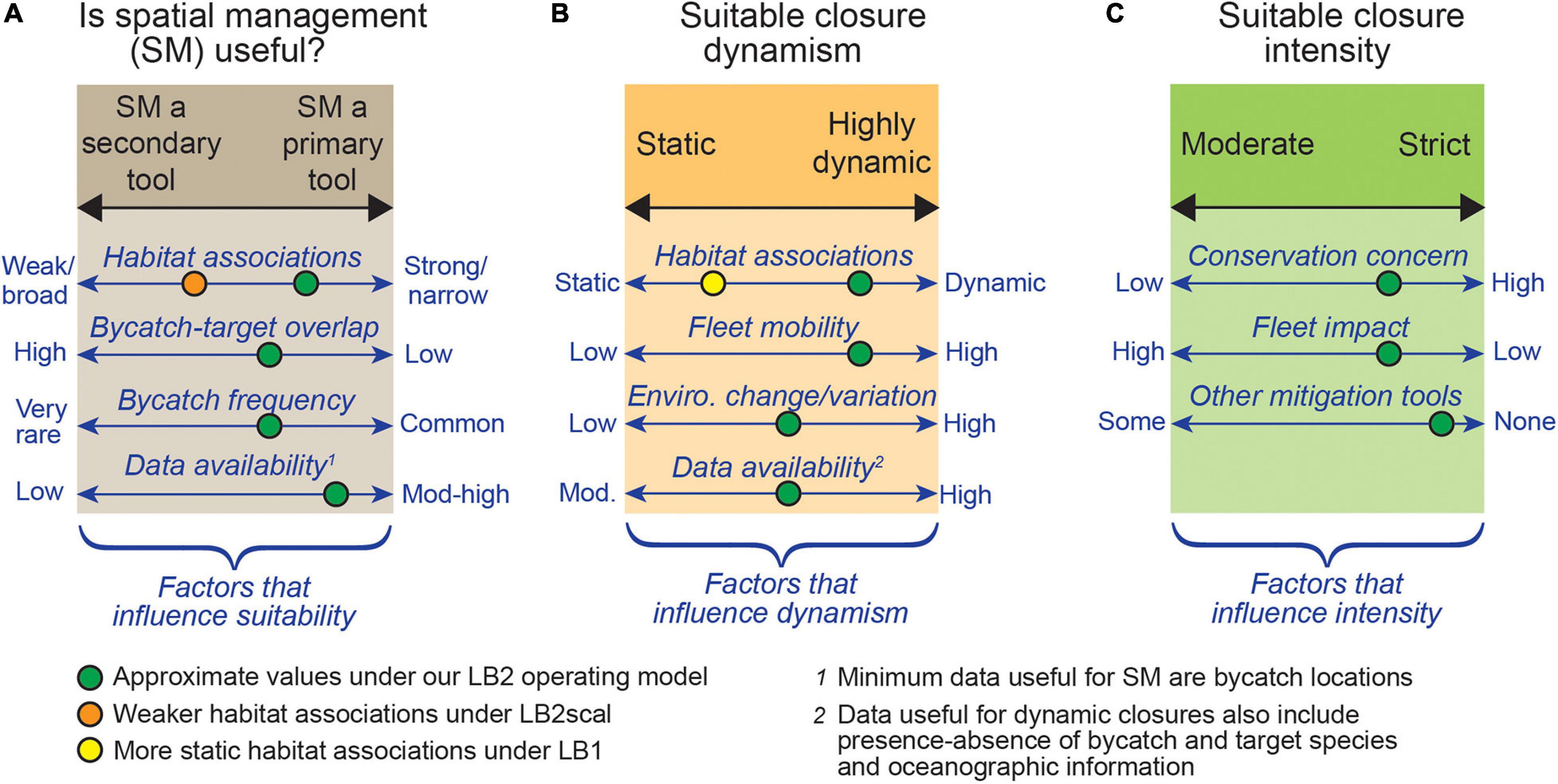
Figure 8. A summary schematic of the key factors indicating when spatial management (SM) is likely to be effective for bycatch mitigation (A), and a set of key factors influencing closure dynamism (ranging from static to highly dynamic; B) and closure intensity (moderate to strict; C). For example, in our simulation the dynamic Dyn-turt_s closure was most successful under the LB2 operating model (green circles), due to a dynamic leatherback distribution, high fleet mobility, and moderate-high data availability (reduced only due to species rarity). A strict threshold was considered effective, due to the high conservation status of leatherbacks, and due to a low fleet impact relative to other closure scenarios. Our LB2scal operating model, which simulated a broader leatherback niche, represented an environment less suited to spatial management (orange circle), due to the reduced ability to relocate fishing effort from high-risk to low-risk areas. This schematic is intended to summarize the key factors contributing to closure success, and these axes could be used to help direct early discussion of the suitability of dynamic closures for other fisheries (but are not a replacement for quantitative analysis). For example, a fishery well suited for dynamic spatial management would have well defined and dynamic distributions of target and bycatch species, and a fleet capable of being redistributed (without great economic impact).

Static or Dynamic?

We found that closure performance depended on the distribution of the species and the distribution of fishers. Static closures were most successful for species with strong geographic associations (LB1) and least successful for more dynamic species distributions (LB2). Static closures were also less successful when they affected popular ports with lower vessel mobility (LB2). Static closures were effective at some objectives, with both the Static-obs_s and Static-pred static closures achieving near-best leatherback bycatch reduction for LB1. The Static-pred closure had less impact on swordfish catch than Static-obs_s, so was overall the best performing static closure (and occasionally with dimensions remarkably similar to the existing PLCA, Supplementary Figure 6.6). The success of the Static-pred closure highlights the value of considering the bycatch risk relative to fishing effort (Static-pred) rather than closing the area with most observed bycatch (Static-obs). This is because the latter approach can cause redistribution of fishing into higher risk areas and simply shift the bycatch elsewhere (O’Keefe et al., 2014; Hoos et al., 2019). Static-pred requires locations of fishing events whether bycatch was caught or not, whereas Static-obs requires only the location of bycatch. This means that Static-obs requires less information and may be more easily created for fisheries with less monitoring. However, the risk of unintended impacts from effort redistribution under Static-obs is such that we encourage that (for comparison with Static-obs closures) Static-pred closures be developed using pseudo-absences (Barbet-Massin et al., 2012) throughout the fishable domain.

Dynamic closures were clearly able to provide more balance between target catch and bycatch, and over time provided similar access to fishing grounds as the no closure strategy (Figure 6). Dynamic closures did require a flexible fleet that was able to fish any location reasonably accessible from port, and dynamic closures may be most successful under conditions of low fishing effort to avoid over-crowding in open pockets. There are practical challenges to dynamic closures as well, for both managers and fishers. For example, we used EcoCast to create dynamic closures at the native scale of ROMS (0.1°) in contrast to the current 0.25° version of EcoCast (Hazen et al., 2018; Welch et al., 2019a), which meant closures had a very fine spatial and temporal resolution. These closures may be difficult to enforce, challenging to communicate and deliver to stakeholders, and fragmented open areas may be difficult for fishers to locate and remain within. There is a spectrum of ‘dynamic’ between completely static and highly dynamic time-area closures, such as event-triggered static closures (Welch et al., 2019b) and threshold type closures (Hobday and Hartmann, 2006). There is much to be gained by exploring these options, especially when there is sufficient data to quantify species distributions, but it is also essential to understand the distribution and redistribution of fishing effort (Powers and Abeare, 2009) and vessel mobility in order to take full advantage of dynamic spatial management. Regarding the current spatial closures used in the DGN (especially the PLCA), our study indicates great potential for increased closure dynamism due to the extensive observer program and availability of ocean data, but incorporating precautionary ‘strict’ closure thresholds (given the high conservation concern for sea turtles) and a multi-tool approach given the very rare occurrence of turtle bycatch (Figure 8).

Species with predictable distributions are most likely to benefit from tailored spatial protection (Hyrenbach et al., 2000; Boerder et al., 2019), but the nature of the predictability influences the success of dynamic closures. Although both static and dynamic closures were somewhat effective for LB1, static closures were largely ineffective at bycatch reduction for LB2. This indicates that the spatial structure of the species’ distribution matters, and species with identifiable habitat but weaker geographic associations may benefit most from dynamic tailored closures. The perfect information closure (Dyn-turt_sP) highlighted the importance of predictive power, as it achieved best bycatch reduction, but there were other important considerations. We saw different predictive performance in the leatherback models fitted to simulated observer data, in LB1 (AUC = 0.82) and LB2 (AUC = 0.66; Supplementary Table 3.1), yet the closures created from these models achieved similar reduction in bycatch risk (leatherbacks per set; Figure 5). This was likely due to the closures in LB2 redistributing more effort (especially from the San Diego port), indicating that a less accurate closure can still achieve good bycatch avoidance by redistributing more effort.

In general, dynamic spatial closures will be most suitable for a fishery in which (Figure 8): bycatch and target species have strong preferences for specific dynamic habitats and have low spatial overlap; bycatch is relatively common (to accurately estimate bycatch risk, and as evidence that redistributing effort can reduce bycatch); ocean and fishery data availability is high; fleet mobility is high (to respond to varying closures); and environmental variation is high (leading to a variable species distribution that requires dynamic closures). Strict dynamic closures are also more likely to be appropriate when the bycatch species is/are of high conservation concern, when fleet impact (namely economic) is comparatively low, and when there are no other suitable bycatch mitigation tools. A fishery least suitable for dynamic closures as a primary tool will have the opposite, with broad, static, strongly overlapping or highly uncertain distributions of bycatch and target species, and a fleet that cannot respond to closure changes without severe economic impacts.

Single or Multi-Species?

Our simulation did not explore multispecies issues in great detail, but it was clear that dynamic closures in this study could not efficiently reduce bycatch of both leatherbacks and blue sharks. Only when a closure was very large, causing the loss of some fishing effort, was bycatch for both species reduced (Dyn-multi_s and LB2; Figure 7). The viability of multi-species protection will be case specific, and depend on the overlap of the species’ distributions as well as the algorithm used for this multi-feature prioritization problem (Welch et al., 2020). Dynamic spatial management is a developing tool for mitigating multi-species bycatch (Little et al., 2015). Our results, however, indicate that if dynamic closures are aimed at reducing bycatch of specific species (rather than bycatch of any species) then incorporating more than a few species in closure design may lead to ‘diminishing returns’ in bycatch reduction (Welch et al., 2020). The advantages of dynamic closures in our study were predominantly for closures weighted to a single species, and more research is needed simulating dynamic closures for a variety of species with different rarity, habitat associations, and home range size. This will help identify the opportunities and limitations in multi-species spatial management.

Bycatch Avoidance, Reduction, or Target-Level?

There are two distinct processes relevant to bycatch mitigation using spatial management: the redistribution of fishing effort, and the reduction of total fishing effort. Time-area closures will cause the first and can lead to the latter when the closure is prohibitively large. Here, we discuss when, and how, time-area closures are likely to be effective bycatch mitigation tools given only redistribution of effort, and consider effort reduction a separate tool.

Time-area closures will be effective at reducing bycatch when effort can be redistributed to locations with lower bycatch risk (Murray et al., 2000; Powers and Abeare, 2009; Hoos et al., 2019). The long-run effectiveness of this redistribution will be directly proportional to the difference in mean risk between the habitats being fished before and after redistribution. If a species is widely distributed throughout the fishable area, or has more similar suitability throughout the domain (as in LB2scal), or if fishers typically fish low risk habitat in the absence of spatial closures (Keith et al., 2020), then effort redistribution is unlikely to be an effective strategy for bycatch reduction. However, bycatch reduction is only one objective, and our analysis highlighted the value of evaluating bycatch reduction alongside other objectives. We thus distinguish three management objectives: bycatch avoidance, bycatch reduction, and target-level bycatch reduction. ‘Avoidance’ refers to closing areas with high bycatch risk regardless of how often they are fished. ‘Reduction’ refers to reducing bycatch rates from current levels, which means at least some fishing must be redistributed to lower risk areas. ‘Target-level reduction’ means reducing bycatch to a specific level (e.g., a specific number of animals or interactions, e.g., a bycatch ‘hard cap’). Determining the appropriate objective influences the types of bycatch mitigation tools used and how spatial management should be used.

The dynamic closure approach we used in our study, i.e., using SDMs to avoid species, is certainly effective for a ‘bycatch avoidance’ objective. This approach identifies and closes the highest risk areas whether they are fished or not. For ‘bycatch reduction’, SDM-based closures can still be effective (e.g., our 30–50% reduction in leatherback bycatch), but calculated closure thresholds need to consider the co-occurrence of species and fishing (e.g., Howell et al., 2015; Eguchi et al., 2017) to ensure some effort is redistributed to lower risk areas. For ‘target-level reduction,’ a different approach is probably required. If the desired level of bycatch is set, say at 10% of current levels, then a closure needs to redistribute effort to specific areas of known (i.e., predicted) bycatch risk. In this case, a better closure design approach would be to identify areas to leave open (rather than areas to close) based on the estimated bycatch given a predicted level of fishing effort in those open areas. For target-level reduction, and for cases in which effort redistribution is unlikely to greatly reduce mean bycatch risk, spatial management is probably best used as a secondary tool to support other management tools, such as effort control, gear modifications and increased gear selectivity, fleet communications, or bycatch quotas (O’Keefe et al., 2014; Senko et al., 2014; Swimmer et al., 2017; Sepulveda and Aalbers, 2018; Holland and Martin, 2019).

Challenges for Dynamic Closures

Our study highlighted some issues for dynamic spatial management that deserve further evaluation, relevant to closure design, implementation, and simulation. A key challenge for designing time-area closures will always be gathering sufficient data on the distribution of species (especially rare species). In our study, 20% observer coverage was sufficient to create useful models of species’ distributions with 5 years of data. This was also close to the minimum coverage required to create a robust SDM, given our specified bycatch rate. Less information, due to a lower bycatch rate or less observer coverage, would likely require simpler SDMs, which may reduce predictive power and closure accuracy. A useful level of observer coverage depends on bycatch rate (Curtis and Carretta, 2020), so while 20% was useful in our simulation it is likely too low to create complex SDMs for the rarest bycatch species in the actual DGN. EcoCast currently creates SDMs from both fishery-dependent data and telemetry data (Hazen et al., 2018), and in the case of species encountered very rarely (e.g., leatherback turtles) relies only on the telemetry. Telemetry data are essential for informing habitat suitability for rarely encountered species, and while these data can indicate the probability of presence they may not accurately indicate catchability and thus the probability of being caught. This may be especially important of probability of presence is used (linearly) to determine closure thresholds. Thus, important research avenues are continued investigation of biases associated with using telemetry data to inform bycatch risk (Žydelis et al., 2011), and exploring modeling approaches for integrating diverse data sources (Grüss and Thorson, 2019) to integrate telemetry and fishery-dependent catch data.

The environment was often a key driver of variation in catch and bycatch (Supplementary Figure 6.10), so the more accurately we can observe and model ocean change, species distributions, and population abundance, the more effective dynamic spatial management will be. But stochasticity was another key component of this variation, arising predominantly from how we sampled integer catches and which fishing sets were observed. Rarer bycatch events will tend to represent the mean risk with reduced precision (Martin et al., 2015), which will typically lead to increased uncertainty in developing spatial closures in the short term. We observed this uncertainty even in the ‘perfect knowledge’ closure, which had perfect knowledge of the mean catch rate only, and the integer catches given that mean were random. There may be other statistical approaches for simulating catches that identify this uncertainty differently (such as using mixture models as operating models), but it may also be that dynamic closures aimed at reducing very rare bycatch events are subject to strong stochasticity (Figure 8). This unavoidable uncertainty should be reflected in the resolution of the closure or in the general management approach (e.g., whether time-area closures are used in concert with other tools).

A valuable research priority is if, and how, closure resolution should reflect model uncertainty. Practical considerations relevant to enforcement and fisher planning will influence the resolution and design of dynamic closures, as should the magnitude, periodicity, and predictability of bycatch (Dunn et al., 2011; Welch et al., 2018). But incorporating model uncertainty in the temporal and spatial resolution of a closure will be more challenging. It seems intuitive that increased uncertainty in a species’ distribution and catchability would encourage a coarser resolution of a dynamic closure; e.g., if the predicted bycatch risk at two locations (or dates) cannot be distinguished with statistical clarity, then they should share the same open/closed status. Further research is needed on the scales of SDM predictability, and temporally and spatially structured cross-validation procedures (Roberts et al., 2017) or spatial autocorrelation analysis (Dunn et al., 2011) may be a useful avenues for quantifying the relationship between predictive power and closure resolution. Advancing the measurement and communication of uncertainty in bycatch risk, alongside the integration of real-time and forecast ocean and bycatch data, will help ensure that dynamic spatial closures make a robust contribution to the management of bycatch in dynamic environments.

Data Availability Statement

The ROMS data are available from oceanmodeling.ucsc.edu. The observer and commercial fisheries data were provided under a confidentiality agreement and cannot be made publicly available. Requests to access the observer data should be directed to the Charles Villafana (Charles.Villafana@noaa.gov) at the West Coast Region Observer Program. Requests to access the commercial landings data should be made to the Pacific Fisheries Information Network (pacfin.psmfc.org).

Ethics Statement

Ethical review and approval was not required for the animal study because Animal locations were derived from commercial fisheries data.

Author Contributions

JS performed the analysis and wrote the first draft of the manuscript. All the authors conceived and designed the study, contributed to the interpretation of results and manuscript revision, and approved the submitted manuscript.

Funding

Funding was provided by the NOAA Climate Program Office Coastal and Ocean Climate Applications (COCA) program (NA17OAR4310268).

Conflict of Interest

The authors declare that the research was conducted in the absence of any commercial or financial relationships that could be construed as a potential conflict of interest.

Acknowledgments

This study used commercial catch data supplied by the Pacific Fisheries Information Network (PacFIN), with agreement from the California Department of Fish and Wildlife (CDFW), the Oregon DFW, and Washington DFW. We are grateful to Jenny Suter, Robert Ryznar, Brad Stenberg, Debbie Aseltine-Neilson, Chris Edwards, John Rakitan, Liz Hellmers, Corey Niles, and Justin Ainsworth for assistance with data access. We recognize the valuable information and insight provided by fishers and other stakeholders during surveys, meetings, and discussions, which informed our efforts to develop a realistic model of fishery operation and fisher behavior.

Supplementary Material

The Supplementary Material for this article can be found online at: https://www.frontiersin.org/articles/10.3389/fmars.2021.630607/full#supplementary-material

Footnotes

1. ^ https://oceanmodeling.ucsc.edu/

References

Armsworth, P. R., Block, B. A., Eagle, J., and Roughgarden, J. E. (2010). The economic efficiency of a time–area closure to protect spawning bluefin tuna. Journal of Applied Ecology 47, 36–46. doi: 10.1111/j.1365-2664.2009.01738.x

CrossRef Full Text | Google Scholar

Barbet-Massin, M., Jiguet, F., Albert, C. H., and Thuiller, W. (2012). Selecting pseudo-absences for species distribution models: how, where and how many? Methods in Ecology and Evolution 3, 327–338. doi: 10.1111/j.2041-210X.2011.00172.x

CrossRef Full Text | Google Scholar

Benson, S. R., Eguchi, T., Foley, D. G., Forney, K. A., Bailey, H., Hitipeuw, C., et al. (2011). Large-scale movements and high-use areas of western Pacific leatherback turtles, Dermochelys coriacea. Ecosphere 2, art84. doi: 10.1890/es11-00053.1

CrossRef Full Text | Google Scholar

Boerder, K., Schiller, L., and Worm, B. (2019). Not all who wander are lost: Improving spatial protection for large pelagic fishes. Marine Policy 105, 80–90. doi: 10.1016/j.marpol.2019.04.013

CrossRef Full Text | Google Scholar

Breiman, L. (2001). Random Forests. Machine Learning 45, 5–32. doi: 10.1023/A:1010933404324

CrossRef Full Text | Google Scholar

Carretta, J. V. (2018). A machine-learning approach to assign species to ‘unidentified’ entangled whales. Endangered Species Research 36, 89–98.

Google Scholar

Chan, H. L., and Pan, M. (2016). Spillover effects of environmental regulation for sea turtle protection in the Hawaii longline swordfish fishery. Marine Resource Economics 31, 259–279.

Google Scholar

Chavez, F. P., Collins, C. A., Huyer, A., and Mackas, D. L. (2002). El Niño along the west coast of North America, Editorial. Prog. Oceanogr 54, 1–5.

Google Scholar

Curtis, K. A., and Carretta, J. V. (2020). ObsCovgTools: Assessing observer coverage needed to document and estimate rare event bycatch. Fisheries Research 225, 105493. doi: 10.1016/j.fishres.2020.105493

CrossRef Full Text | Google Scholar

Dinmore, T. A., Duplisea, D. E., Rackham, B. D., Maxwell, D. L., and Jennings, S. (2003). Impact of a large-scale area closure on patterns of fishing disturbance and the consequences for benthic communities. ICES Journal of Marine Science 60, 371–380. doi: 10.1016/s1054-3139(03)00010-9

CrossRef Full Text | Google Scholar

Dunn, D. C., Boustany, A. M., and Halpin, P. N. (2011). Spatio-temporal management of fisheries to reduce by-catch and increase fishing selectivity. Fish and Fisheries 12, 110–119. doi: 10.1111/j.1467-2979.2010.00388.x

CrossRef Full Text | Google Scholar

Dunn, D. C., Maxwell, S. M., Boustany, A. M., and Halpin, P. N. (2016). Dynamic ocean management increases the efficiency and efficacy of fisheries management. Proceedings of the National Academy of Sciences 113, 668–673. doi: 10.1073/pnas.1513626113

PubMed Abstract | CrossRef Full Text | Google Scholar

Eguchi, T., Benson, S. R., Foley, D. G., and Forney, K. A. (2017). Predicting overlap between drift gillnet fishing and leatherback turtle habitat in the California Current Ecosystem. Fisheries Oceanography 26, 17–33. doi: 10.1111/fog.12181

CrossRef Full Text | Google Scholar

Elkan, C. (2001). “The foundations of cost-sensitive learning,” in Proceedings of the 17th International joint conference on artificial intelligence (Seattle, WA), 973–978.

Google Scholar

Goodyear, C. P. (1999). An analysis of the possible utility of time-area closures to minimize billfish bycatch by U.S. pelagic longlines. Fish. Bull. US 97, 243–255.

Google Scholar

Grantham, H. S., Petersen, S. L., and Possingham, H. P. (2008). Reducing bycatch in the South African pelagic longline fishery: the utility of different approaches to fisheries closures. Endangered Species Research 5, 291–299. doi: 10.3354/esr00159

CrossRef Full Text | Google Scholar

Grüss, A., and Thorson, J. T. (2019). Developing spatio-temporal models using multiple data types for evaluating population trends and habitat usage. ICES Journal of Marine Science 76, 1748–1761. doi: 10.1093/icesjms/fsz075

CrossRef Full Text | Google Scholar

Hall, M. A., Alverson, D. L., and Metuzals, K. I. (2000). By-Catch: problems and solutions. Marine Pollution Bulletin 41, 204–219. doi: 10.1016/S0025-326X(00)00111-9

CrossRef Full Text | Google Scholar

Hazen, E. L., Scales, K. L., Maxwell, S. M., Briscoe, D. K., Welch, H., Bograd, S. J., et al. (2018). A dynamic ocean management tool to reduce bycatch and support sustainable fisheries. Science Advances 4, eaar3001. doi: 10.1126/sciadv.aar3001

PubMed Abstract | CrossRef Full Text | Google Scholar

Helvey, M., Pomeroy, C., Pradhan, N. C., Squires, D., and Stohs, S. (2017). Can the United States have its fish and eat it too? Marine Policy 75, 62–67. doi: 10.1016/j.marpol.2016.10.013

CrossRef Full Text | Google Scholar

Hobday, A. J., and Hartmann, K. (2006). Near real-time spatial management based on habitat predictions for a longline bycatch species. Fisheries Management and Ecology 13, 365–380. doi: 10.1111/j.1365-2400.2006.00515.x

CrossRef Full Text | Google Scholar

Holland, D. S., and Martin, C. (2019). Bycatch Quotas, Risk Pools, and Cooperation in the Pacific Whiting Fishery. Frontiers in Marine Science 6:600. doi: 10.3389/fmars.2019.00600

CrossRef Full Text | Google Scholar

Holts, D., and Sosa-Nishizaki, O. (1998). Swordfish, Xiphias gladius, Fisheries of the Eastern North Pacific Ocean. In Biology and Fisheries of Swordfish, Xiphias gladius. NOAA Technical Report NMFS 142. Seattle, WA: U.S. Department of Commerce, 65–76.

Google Scholar

Hoos, L. A., Buckel, J. A., Boyd, J. B., Loeffler, M. S., and Lee, L. M. (2019). Fisheries management in the face of uncertainty: designing time-area closures that are effective under multiple spatial patterns of fishing effort displacement in an estuarine gill net fishery. PLoS One 14:e0211103. doi: 10.1371/journal.pone.0211103

PubMed Abstract | CrossRef Full Text | Google Scholar

Howell, E. A., Hoover, A., Benson, S. R., Bailey, H., Polovina, J. J., Seminoff, J. A., et al. (2015). Enhancing the TurtleWatch product for leatherback sea turtles, a dynamic habitat model for ecosystem-based management. Fisheries Oceanography 24, 57–68. doi: 10.1111/fog.12092

CrossRef Full Text | Google Scholar

Howell, E. A., Kobayashi, D. R., Parker, D. M., Balazs, G. H., and Polovina, J. J. (2008). TurtleWatch: a tool to aid in the bycatch reduction of loggerhead turtles Caretta caretta in the Hawaii-based pelagic longline fishery. Endangered Species Research 5, 267–278.

Google Scholar

Hyrenbach, K. D., Forney, K. A., and Dayton, P. K. (2000). Marine protected areas and ocean basin management. Aquatic Conservation. Marine and Freshwater Ecosystems 10, 437–458. doi: 10.1002/1099-0755(200011/12)10:6<437::Aid-aqc425>3.0.Co;2-q

CrossRef Full Text | Google Scholar

Keith, D. M., Sameoto, J. A., Keyser, F. M., and Ward-Paige, C. A. (2020). Evaluating socio-economic and conservation impacts of management: A case study of time-area closures on Georges Bank. PLoS One 15:e0240322. doi: 10.1371/journal.pone.0240322

PubMed Abstract | CrossRef Full Text | Google Scholar

Lewison, R., Hobday, A. J., Maxwell, S., Hazen, E., Hartog, J. R., Dunn, D. C., et al. (2015). Dynamic ocean management: identifying the critical ingredients of dynamic approaches to ocean resource management. BioScience 65, 486–498. doi: 10.1093/biosci/biv018

CrossRef Full Text | Google Scholar

Lewison, R. L., Crowder, L. B., Wallace, B. P., Moore, J. E., Cox, T., Zydelis, R., et al. (2014). Global patterns of marine mammal, seabird, and sea turtle bycatch reveal taxa-specific and cumulative megafauna hotspots. Proceedings of the National Academy of Sciences 111, 5271–5276. doi: 10.1073/pnas.1318960111

PubMed Abstract | CrossRef Full Text | Google Scholar

Little, A. S., Needle, C. L., Hilborn, R., Holland, D. S., and Marshall, C. T. (2015). Real-time spatial management approaches to reduce bycatch and discards: experiences from Europe and the United States. Fish and Fisheries 16, 576–602. doi: 10.1111/faf.12080

CrossRef Full Text | Google Scholar

Martin, S. L., Stohs, S. M., and Moore, J. E. (2015). Bayesian inference and assessment for rare-event bycatch in marine fisheries: a drift gillnet fishery case study. Ecological Applications 25, 416–429. doi: 10.1890/14-0059.1

CrossRef Full Text | Google Scholar

Mason, J. G., Hazen, E. L., Bograd, S. J., Dewar, H., and Crowder, L. B. (2019). Community-level effects of spatial management in the California drift gillnet Fishery. Fisheries Research 214, 175–182. doi: 10.1016/j.fishres.2019.02.010

CrossRef Full Text | Google Scholar

Maxwell, S. M., Hazen, E. L., Lewison, R. L., Dunn, D. C., Bailey, H., Bograd, S. J., et al. (2015). Dynamic ocean management: Defining and conceptualizing real-time management of the ocean. Marine Policy 58, 42–50. doi: 10.1016/j.marpol.2015.03.014

CrossRef Full Text | Google Scholar

Murray, K. T., Read, A. J., and SoLow, A. R. (2000). The use of time/area closures to reduce bycatches of harbour porpoises: lessons from the Gulf of Maine sink gillnet fishery. Journal of Cetacean Research and Management 2, 135–141.

Google Scholar

Neveu, E., Moore, A. M., Edwards, C. A., Fiechter, J., Drake, P., Crawford, W. J., et al. (2016). An historical analysis of the California Current circulation using ROMS 4D-Var: System configuration and diagnostics. Ocean Modelling 99, 133–151. doi: 10.1016/j.ocemod.2015.11.012

CrossRef Full Text | Google Scholar

Oestreich, W. K., Chapman, M. S., and Crowder, L. B. (2020). A comparative analysis of dynamic management in marine and terrestrial systems. Frontiers in Ecology and the Environment 18:496–504. doi: 10.1002/fee.2243

CrossRef Full Text | Google Scholar

O’Keefe, C. E., Cadrin, S. X., and Stokesbury, K. D. E. (2014). Evaluating effectiveness of time/area closures, quotas/caps, and fleet communications to reduce fisheries bycatch. ICES Journal of Marine Science 71, 1286–1297. doi: 10.1093/icesjms/fst063

CrossRef Full Text | Google Scholar

Powers, J. E., and Abeare, S. M. (2009). Fishing effort redistribution in response to area closures. Fisheries Research 99, 216–225. doi: 10.1016/j.fishres.2009.06.011

CrossRef Full Text | Google Scholar

Punt, A. E., Butterworth, D. S., de Moor, C. L., De Oliveira, J. A. A., and Haddon, M. (2016). Management strategy evaluation: best practices. Fish and Fisheries 17, 303–334. doi: 10.1111/faf.12104

CrossRef Full Text | Google Scholar

R Core Team. (2020). R: A language and environment for statistical computing. Vienna: R Foundation for Statistical Computing.

Google Scholar

Roberts, D. R., Bahn, V., Ciuti, S., Boyce, M. S., Elith, J., Guillera-Arroita, G., et al. (2017). Cross-validation strategies for data with temporal, spatial, hierarchical, or phylogenetic structure. Ecography 40, 913–929. doi: 10.1111/ecog.02881

CrossRef Full Text | Google Scholar

Savoca, M. S., Brodie, S., Welch, H., Hoover, A., Benaka, L. R., Bograd, S. J., et al. (2020). Comprehensive bycatch assessment in US fisheries for prioritizing management. Nature Sustainability 3, 472–480. doi: 10.1038/s41893-020-0506-9

CrossRef Full Text | Google Scholar

Senko, J., White, E. R., Heppell, S. S., and Gerber, L. R. (2014). Comparing bycatch mitigation strategies for vulnerable marine megafauna. Animal Conservation 17, 5–18. doi: 10.1111/acv.12051

CrossRef Full Text | Google Scholar

Sepulveda, C. A., and Aalbers, S. A. (2018). Exempted Testing of Deep-set Buoy Gear and Concurrent Research Trials on Swordfish, Xiphias gladius, in the Southern California Bight. Marine Fisheries Review 80, 17–29.

Google Scholar

Smith, J. A., Tommasi, D., Sweeney, J., Brodie, S., Welch, H., Hazen, E. L., et al. (2020). Lost opportunity: Quantifying the dynamic economic impact of time-area fishery closures. Journal of Applied Ecology 57, 502–513. doi: 10.1111/1365-2664.13565

CrossRef Full Text | Google Scholar

Stock, B. C., Ward, E. J., Eguchi, T., Jannot, J. E., Thorson, J. T., Feist, B. E., et al. (2019). Comparing predictions of fisheries bycatch using multiple spatiotemporal species distribution model frameworks. Canadian Journal of Fisheries and Aquatic Sciences 77, 146–163. doi: 10.1139/cjfas-2018-0281

CrossRef Full Text | Google Scholar

Stock, B. C., Ward, E. J., Thorson, J. T., Jannot, J. E., and Semmens, B. X. (2018). The utility of spatial model-based estimators of unobserved bycatch. ICES Journal of Marine Science 76, 255–267. doi: 10.1093/icesjms/fsy153

CrossRef Full Text | Google Scholar

Swimmer, Y., Gutierrez, A., Bigelow, K., Barceló, C., Schroeder, B., Keene, K., et al. (2017). Sea Turtle Bycatch Mitigation in U.S. Longline Fisheries. Frontiers in Marine Science 4:260. doi: 10.3389/fmars.2017.00260

CrossRef Full Text | Google Scholar

Urbisci, L. C., Stohs, S. M., and Piner, K. R. (2016). From sunrise to sunset in the California Drift Gillnet Fishery: an examination of the effects of time and area closures on the catch and catch rates of pelagic species. Marine Fisheries Review 78, 1–11. doi: 10.7755/MFR.78.3-4.1

CrossRef Full Text | Google Scholar

van Putten, I. E., Kulmala, S., Thébaud, O., Dowling, N., Hamon, K. G., Hutton, T., et al. (2012). Theories and behavioural drivers underlying fleet dynamics models. Fish and Fisheries 13, 216–235. doi: 10.1111/j.1467-2979.2011.00430.x

CrossRef Full Text | Google Scholar

Welch, H., Brodie, S., Jacox, M. G., Bograd, S. J., and Hazen, E. L. (2020). Decision-support tools for dynamic management. Conservation Biology 34, 589–599. doi: 10.1111/cobi.13417

PubMed Abstract | CrossRef Full Text | Google Scholar

Welch, H., Hazen, E. L., Bograd, S. J., Jacox, M. G., Brodie, S., Robinson, D., et al. (2019a). Practical considerations for operationalizing dynamic management tools. Journal of Applied Ecology 56, 459–469. doi: 10.1111/1365-2664.13281

CrossRef Full Text | Google Scholar

Welch, H., Hazen, E. L., Briscoe, D. K., Bograd, S. J., Jacox, M. G., Eguchi, T., et al. (2019b). Environmental indicators to reduce loggerhead turtle bycatch offshore of Southern California. Ecological Indicators 98, 657–664. doi: 10.1016/j.ecolind.2018.11.001

CrossRef Full Text | Google Scholar

Welch, H., Pressey, R. L., and Reside, A. E. (2018). Using temporally explicit habitat suitability models to assess threats to mobile species and evaluate the effectiveness of marine protected areas. Journal for Nature Conservation 41, 106–115. doi: 10.1016/j.jnc.2017.12.003

CrossRef Full Text | Google Scholar

Žydelis, R., Lewison, R. L., Shaffer, S. A., Moore, J. E., Boustany, A. M., Roberts, J. J., et al. (2011). Dynamic habitat models: using telemetry data to project fisheries bycatch. Proceedings of the Royal Society B: Biological Sciences 278, 3191–3200. doi: 10.1098/rspb.2011.0330

PubMed Abstract | CrossRef Full Text | Google Scholar