Abiotic and Human Drivers of Reef Habitat Complexity Throughout the Main Hawaiian Islands

Introduction

Habitat complexity is the three-dimensional (3D) structure of the physical environment with which organisms interact and is a key influencer of the distribution of marine biota. Habitat complexity can affect a variety of ecological functions such as by providing prey protection from predators, surfaces for coral settlement and growth, and different microhabitats to support a variety of species. Habitat complexity interacts with other environmental factors such as light, temperature and wave action to generate a wide range of ecological conditions (Sebens, 1991).

On coral reefs, 3D habitat complexity is a determinant of reef fish assemblages, where fish abundance, biomass, and richness are often positively correlated with complexity (Cinner et al., 2009; Graham et al., 2009). Yet the direction and strength of this relationship does vary, and studies can also show mixed connectivity between reef complexity and fish stocks (Jennings et al., 1996; Harborne et al., 2012). Coral cover is also often positively correlated with reef complexity (Alvarez-Filip et al., 2009; Graham and Nash, 2012). Correspondingly, negative relationships between complexity and algal cover often exist, perhaps indirectly reflecting the role of reef complexity in predicting reef fish and resulting herbivory (Graham and Nash, 2012). However, 3D habitat complexity is not only driven by coral cover, but also by benthic geomorphology at a range of scales from small boulder and erosion-deposition zones to large subsurface geologic structures.

The Main Hawaiian Islands (MHIs) are an important case-in-point, varying widely in geologic age from less than a few years old on Hawai‘i Island to more than six million years old on Ni‘ihau (Neall and Trewick, 2008). Island age is accompanied by stage of accretion and subsidence, processes that generate enormous inter- and intra-island variation in reef extent associated with benthic substrate availability (Asner et al., 2020b). Younger islands such as Hawai‘i contain vast fringing reefs dominated by rock substrates (i.e., lava beds, massive boulders, rock fields) that define much of the reef rugosity, but with embayments and coves co-dominated by geology and coral growth. In contrast, older islands such as Kaua‘i and O‘ahu contain reefs defined by geologic subsidence and erosional surfaces, with broad expanses of both sandy bottom and calcareous reef substrate.

Overlain on this geologic template, water motion and light penetration decrease with increasing depth, and wave-sheltered areas show the greatest Holocene reef accretion (Grigg, 1998). Generally, optimal reef growth occurs between 10 and 20 m depth in the MHI, reflecting a trade-off between wave-induced stress and decreased light availability (Storlazzi et al., 2005). In areas of greatest wave power, turf algae and crustose coralline algae dominate due to more wave-tolerant, flatter morphologies. On the other hand, low wave power regions are dominated by hard corals and macroalgae with structures more vulnerable to dislodgement (Engelen et al., 2005; Madin et al., 2014; Gove et al., 2015).

Reef complexity varies over multiple spatial scales (Mumby et al., 2004). Measurements of complexity aim to quantify the vertical variation of the benthic surface in relation to the two-dimensional (2D) surface of the same area, and therefore complexity metrics are dependent upon the resolution of the mapping technique. Larger grid or pixel sizes of bathymetric maps result in complexity values describing broader geological features in comparison to smaller pixel sizes that represent specific coral colonies, rock outcrops and other fine-scale features. Presently, the spatial scale at which biophysical drivers influence fish or invertebrate assemblages is poorly known (Purkis et al., 2008; Aston et al., 2019), and a multi-scale assessment of reef complexity would improve our understanding of habitat across a range of scales relevant to a wide range of ecological processes (Harborne et al., 2006; Williams et al., 2015).

Over the past several decades, there has been a rapid increase in the diversity of methods used to quantify 3D habitat complexity, where various techniques are aimed at quantifying complexity at specific scales and spatial resolutions. Studies focusing on colony-level measures most commonly use a chain-and-tape method to estimate rugosity, an index of habitat complexity. Rugosity is estimated by calculating the ratio of chain length laid across the bottom reef profile to the linear distance of the transect (Risk, 1972). Complexity has also been estimated visually by scoring a range of structural variables (Gratwicke and Speight, 2005). Modern methods of assessing habitat complexity include 3D computer models, which are generated from images via structure-from-motion photogrammetry, allowing quantification of complexity metrics such as surface rugosity among fractal dimension, total surface area and surface height (Burns et al., 2015; Figueira et al., 2015). Field techniques, however, can be time-consuming and typically operate over limited areas (<0.25 ha; Lechene et al., 2019).

Remote sensing methods–primarily acoustic imaging and light detection and ranging (LiDAR)–have allowed estimations of reef complexity over areas of much greater extent. More than 50 years ago, sound navigation and ranging (SONAR) revolutionized reef mapping over large areas by providing moderate resolution information (Moravec and Elfes, 1985). Subsequent LiDAR-derived rugosity measures of reef at 4–5 m spatial resolution have been correlated with in situ measures of reef rugosity (Wedding et al., 2008). However, measurements of habitat complexity coarser than 10 m did not show significant relationships with in situ rugosity, but they still provided relevant information at broader geographic scales (Wedding et al., 2008). Similarly, reef rugosity estimated though acoustic methods showed relationships with fish at kernel sizes less than 40 m, with the most significant relationships with species richness at a resolution finer than 8 m (Purkis et al., 2008). More recently, airborne imaging spectroscopy has opened up access to large-area bathymetric and reef rugosity mapping at resolutions of 0.4 m (Asner et al., 2020a).

Throughout the Hawaiian Islands, it is not known how environmental and physical factors compare with human influences in shaping 3D habitat complexity (Wedding et al., 2018). Understanding controls over spatial patterns of complexity is relevant to creating effective marine managed areas, where planning can benefit fish assemblages, protect essential fish habit and enhance recruitment (Grober-Dunsmore et al., 2007). This is especially important for coastal communities that heavily rely on ecosystem services from reef fish populations. Furthermore, protecting locations with greater reef complexity should be a management priority as they have increased resilience to coral bleaching and enhanced recovery through larger fish populations (Graham and Nash, 2012; Rogers et al., 2014). Considering the wealth of research linking reef complexity and reef fish, rapid methods that can document rugosity at broader geographic scales are of great value. Here we use a new airborne mapping technique to report on how 3D habitat complexity varies at fine and coarse spatial resolutions within and between each Main Hawaiian Island. We undertook this study without a specific focus on live corals, which was largely covered in Asner et al. (2020b). In that earlier paper, we determined the geographic distribution of live corals, but we were unable to associate live coral cover broadly with rugosity due to extremes in island age, geologic stage, and erosional processes. As a result, in the present submission, we determined the geographic distribution of fine- and coarse-scale rugosity surfaces in order to assess on the relative importance of multiple abiotic environmental as well as human factors potentially affecting reef complexity at intra- and inter-island scales.

Materials and Methods

Bathymetric Mapping

Using data collected by the Global Airborne Observatory (Asner et al., 2012), we mapped benthic depth at 2 m spatial resolution throughout the eight MHI. We selected 2 m mapping resolution as a practical trade-off between time and cost of mapping the vast area of the MHI, while simultaneously achieving sufficient resolution to resolve fine-scale variation in reef structure that incorporates larger coral colonies and basaltic rock outcrops (see Asner et al., 2020a). The GAO collected data from multiple coaligned instruments, two of which were used for bathymetric and rugosity mapping: a high-fidelity visible-to-shortwave infrared (VSWIR) imaging spectrometer and a dual-beam LiDAR scanner (Asner et al., 2012). Data from the spectrometer were used to model benthic depth using the deep learning methodology described, tested and validated in Asner et al. (2020a).

The VSWIR spectrometer and LiDAR data were collected between January 2 and February 4, 2019. To maximize data consistency, daily airborne operations were performed from 0830 to 1100 local time. Collection location could change during each flight day and was actively managed based on need, cloud cover, and windspeeds to provide both the most efficient use of time and the best conditions for spectroscopic seafloor measurements. During flight, instrument settings were set for the planned nominal flight altitude of 2 km above the sea surface. Flightlines were spaced to achieve 50% overlap in VSWIR spectrometer coverage. Aircraft ground speed was 130–140 kt. LiDAR pulse frequency was set to 200 kHz (100 kHz per laser) and scan frequency was 34 Hz with a field of view of 38°, allowing 2° of buffer on each side of the spectrometer field of view of 34°, achieving a nominal pulse density of more than 4 pulses m^–2. The radiance data from the spectrometer are collected in 427 spectral channels covering the 350–2500 nm wavelength range in 5 nm increments. Using a modified version of the ATREM model (Gao and Goetz, 1990; Thompson et al., 2017), we retrieved ocean surface reflectance from the at-sensor radiance data. The reflectance data for each flight line were passed through the model described in Asner et al. (2020a) to retrieve estimated depth in meters after masking out problematic regions (clouds, waves, and regions of excessive solar glint) from the data. Because water absorbs nearly all infrared light, land surface objects were filtered from analysis using a reflectance threshold at the 890–910 nm wavelength.

Orthorectification of the spectrometer data was a multi-step process. During flight GPS timing data were collected during flight by both instruments, and this timing location was used to link the data to a precise flight trajectory built from corrected and interpolated data from the onboard positioning and orientation system (POS). With a LiDAR-derived digital surface model (DSM) and a known position and orientation of the sensor at each sample, the 3-dimensional position of each spectrometer pixel was ray-traced to the sea surface level. However, to accurately map the location of each pixel on the ocean floor, we needed to account for estimated depth (d) and the refraction of light at the ocean surface. For each pixel, observation angle from zenith at the water surface, ϕ_a, is known and with standard refractive indices of 1.33000 for water and 1.00029 for air, Snell’s refraction formula can be used to compute the angle after crossing the water surface boundary as ϕ_b = sin⁻¹⁡(0.75210sin⁡ϕ_a). This angle can be traced down to the ocean floor to retrieve the 3-dimensional ocean floor location for each pixel.

We took advantage of the 50% overlap in flight lines to build smooth depth mosaics by reducing sharp transitions between flight lines. For each group of flight lines making up a single region of coastline, the process for mosaicking followed these steps:

(1) Record pixel id, flight line id, depth, and observation zenith angle for up to 5000 (randomly sampled, if more than 5000 are available) pixels that have overlapping flightlines.

(2) For each pixel id, compute the mean and range of measured depth across all overlapping flightlines in addition to the view zenith angle for each flightline.

(3) Compute the mean observation zenith angle for each flight line id and subtract this value from all angle values in the flight line (center the values at 0).

(4) Filter out pixel ids where range > 5.0 m from analysis, as they are likely to be affected by noisy depth retrieval.

(5) For each flight line with valid pixels in overlap area, set up a linear regression with pixel mean depth as dependent variable and terms for intercept, line depth, and mean-centered line observation zenith angle. The fitted coefficients are saved for later use.

(6) Correct all pixel values for each flight line using the linear transformation from the regression fit.

(7) For each mosaic pixel id collect the corrected depths from all overlapping flight lines and compute mean depth.

This was done for each coastal region for each of Ni‘ihau (one region), Kaua‘i (four regions), O‘ahu (four regions), Moloka‘i, Lana‘i, Kaho‘olawe (each one region), Maui (four regions), and Hawai‘i (11 regions). These individual regions were then hand-mosaicked into whole-island maps of depth, with the exception of Hawai‘i which was broken into four quadrants due to size limitations.

Multi-Resolution Rugosity

We computed island-wide maps of rugosity at two resolutions using the “planar” rugosity metric (Jenness, 2004) on the GAO benthic depth maps (Figure 1). Missing data of less than two pixels in width were filled using an inverse-distance weighted average of the three nearest neighboring pixels. Fine-scale rugosity was computed using a 3 × 3 pixel (6 × 6 m) moving window on the original 2 m resolution bathymetric maps (Figure 1b). This resolution seeks high frequency changes on the seafloor arising from coral colonies, rocks, and other bottom features that generate local habitat variability. Coarse-scale rugosity was computed by first down-sampling the 2 m depth maps to 6 m resolution using a mean filter. The planar rugosity metric was then computed using a 9 × 9 pixel (54.0 × 54.0 m) moving window on the 6 m depth maps. Coarse-scale rugosity is responsive to variations in larger terrain features resulting from geologic, reef-scale accretion and subsidence processes. Previous testing at other resolutions indicated that a 9 × 9 pixel coarse-scale rugosity product gives the best detail for geologic features while removing fine-scale “noise” from corals and rock boulders (Figure 1c). These two resolutions of rugosity were computed for each of the individual island depth maps. Because the distribution of rugosity (r) is heavily skewed to the right because of occasional noise pixels, and the units of the output are not meaningful, we transformed raw rugosity values to have an approximate uniform [0,1] distribution T by sorting the n individual values across the map and assigning the value of transformed rugosity $T\left(r_{\text{i}}\right)=\frac{\text{float}\left(\text{rank}\left(r_{\text{i}}\right)\right)}{n}$. Thus, for the island-scale fine and coarse rugosity maps, low transformed rugosity values will be near-zero, mid-range values will be near 0.5, and extreme values will never be more than 1.0.

FIGURE 1

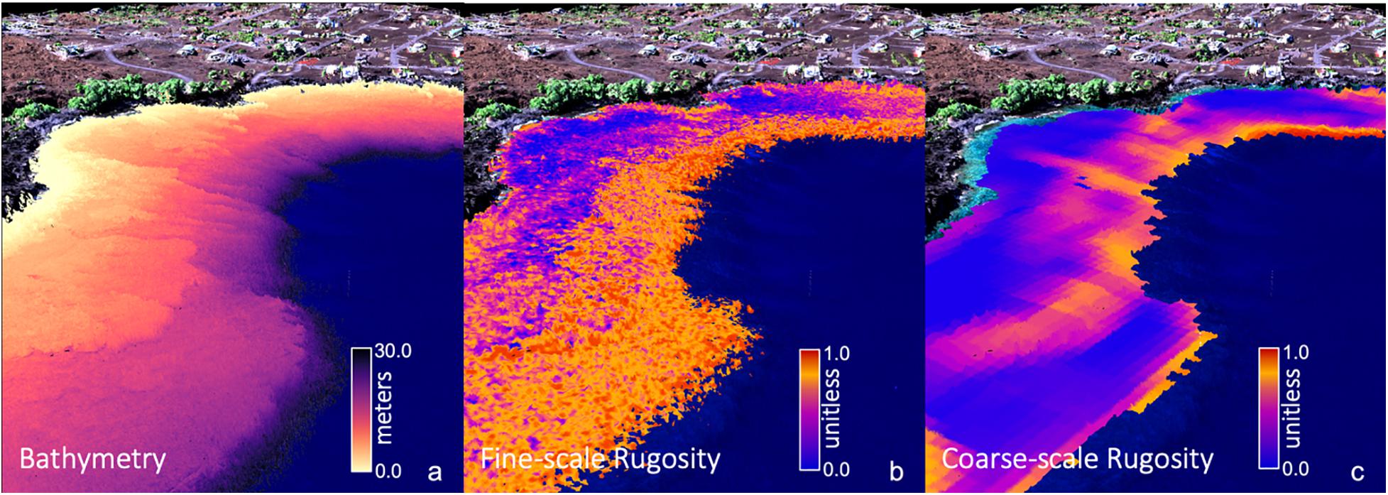
Figure 1. Global Airborne Observatory (GAO) mapping of three-dimensional (a) reef bathymetry, (b) fine-scale rugosity, and (c) coarse-scale rugosity for an embayment along the coast of Hawai‘i Island. Water depth and fine-scale rugosity were mapped at 2 m spatial resolution. Coarse-scale rugosity was mapped at 6 m resolution. Background provides 3D coastline terrain, vegetation and infrastructure as visual reference.

Geospatial Analyses

We assessed the spatial patterning of fine and coarse rugosity both between and within the MHIs using empirical variograms. To overcome computer memory and time limits, we broke the rugosity maps for each island into a grid of 1 × 1 km cells, made up of 500 × 500 pixels for fine rugosity and 167 × 167 pixels for coarse rugosity. Because of the additive nature of the variogram variances, we could compute one for each island using sample-size weighted averages of the individual lag variances across grid cells into a single variogram. This methodology provided the additional benefit of generating information about the variation in spatial patterning within each island.

For each grid cell, the associated square region was extracted from the rugosity map along with a buffer of 500 m (250 pixels for fine-scale maps and 83 pixels for coarse-scale maps) on all sides. The empirical variogram for each grid cell was computed with the GeoStats package (Hoffimann, 2018) in the Julia programming language (Bezanson et al., 2012), using 40 lag steps and a maximum lag of 500 m. A variogram model was fit to the empirical variogram for each grid cell, with the fitting software iterating over eight model forms to find the optimal form as well as the associated optimal estimates for the model parameters: sill, nugget, and range parameters. By storing the sill, nugget, and range value for each parcel, we were able to aggregate these into a 1 × 1 km resolution map of each parameter for each island. The island-wide empirical variogram was computed as a weighted average of the variograms from all grid cells, where the weight for each cell was the number of valid rugosity observations separated by the given lag distance within that cell.

Land-Sea Driver Modeling

We used multiple land-sea environmental maps available for the MHI to assess the relative importance of environmental and human factors that may contribute to the mapped distribution of fine- and coarse-scale rugosity (Table 1). For example, reef depth, slope, and distance to coastline vary with island geologic stage, thereby affecting erosion, subsidence, and other factors known to shape larger benthic structures (Fletcher et al., 2008; Gove et al., 2015). Abiotic drivers also play a role in shaping rugosity, either via physical impacts of waves and wind action (Li et al., 2016), or via the impacts of temperature on calcareous organisms like corals that contribute to rugosity (Ignatov, 2010; Wedding et al., 2018). Finally, nearshore development may have an effect on reef rugosity via sedimentation and/or removal of reef structures (Center for International Earth Science Information Network-Ciesin, 2018). We checked for driver variable co-variance and utilized a combination of drivers each with less than 50% correlation.

TABLE 1

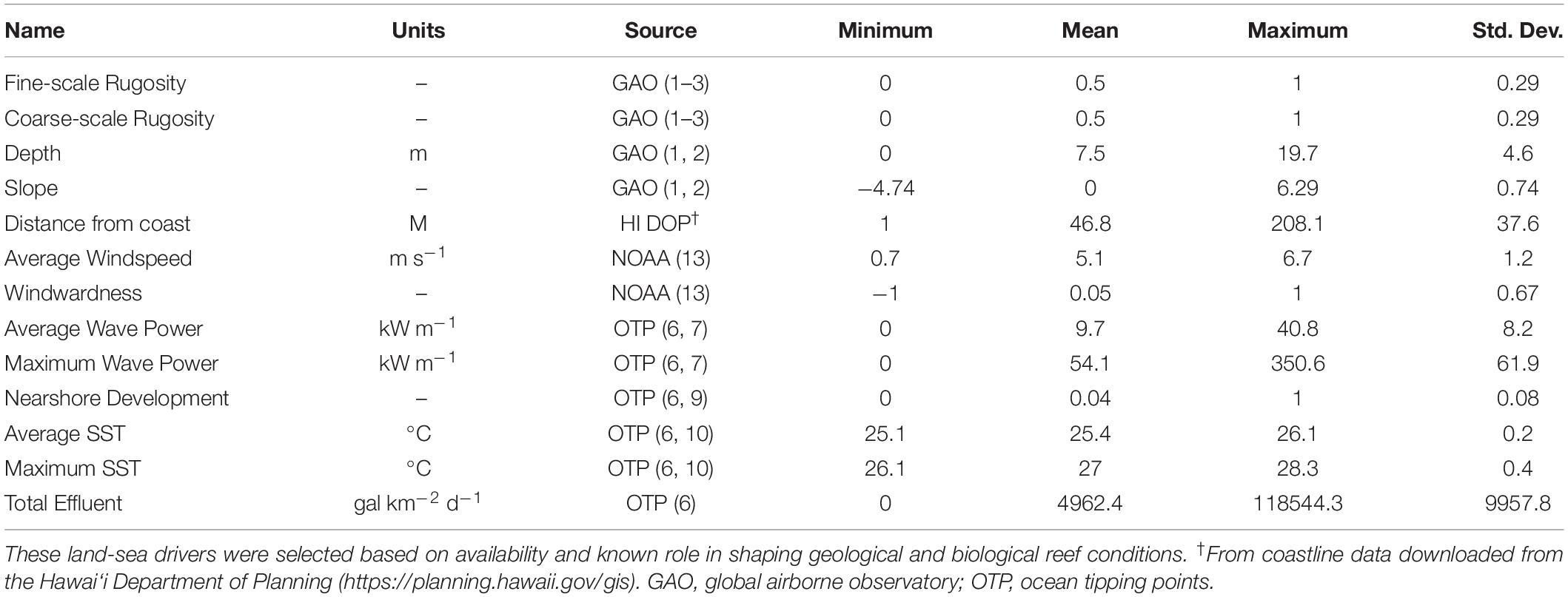
Table 1. Summary statistics for the two mapped rugosity scales as well as 11 factors used in the land-sea driver modeling assessment.

While the GAO fine- and coarse-scale rugosity maps have a resolution of 2 and 6 m, respectively, many of the environmental maps in Table 1 are provided only at resolutions of 30 m or coarser. The GAO rugosity maps were therefore coarsened to 30 m resolution using a mean filter, because we determined this resolution to sufficiently balance the finer and coarser datasets in this analysis. Similarly, all input factors were resampled to match this resolution, using cubic spline interpolation for maps requiring upscaling and a mean filter for maps requiring downscaling. These input factor maps included the GAO bathymetry map used to compute rugosity, as well as slope computed from the 30 m depth map.

We sought to analyze the relative importance and influence of each of these factors on each of the two scales of rugosity at two levels: once separately for each individual island and once for all islands combined. By separating these analyses, we assessed whether drivers of rugosity differ by island while simultaneously revealing general patterns that apply to all islands. We randomly selected 80,000 pixels from the 30 m resampled maps for each individual island and, separately, randomly selected 100,000 pixels across all islands. Modeling was carried out using a Random Forest Machine Learning (RFML) approach (Breiman, 2001) with the Scikit-Learn python package version 0.22.1 (Pedregosa et al., 2011). Optimal settings for the RFML metaparameters defining the number of trees in the forest (“nest”) were discovered through a grid search approach separately for each island (Table 2). We manually specified several metaparameters: four as the maximum tree depth, 1 as the minimum number of samples per leaf, two as the minimum number of samples per split, and four as the maximum number of features scanned at each split. All other meta parameters were left at the default settings. The final model was a descriptive machine learning model, fit to better understand the system rather than be applied to any new data. Because the risk of overfitting is negligible in these circumstances, the idea of parsimony is not applicable and no model simplification procedure was required. With the RF model-fitting procedure, unimportant factors are simply not selected as splitting criteria for many of the node splits that make up each component regression tree. Thus, these factors will have little influence over model capacity to fit the data, and this lack of influence will show as low values in any following assessments of individual factor importance.

TABLE 2

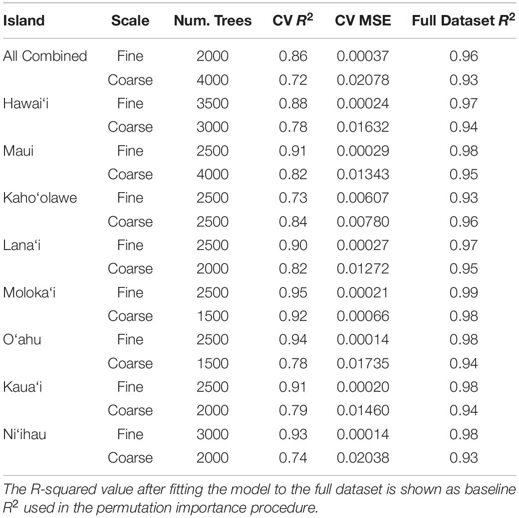
Table 2. Optimized random forest metaparameters used in each individual and combined model from the land-sea driver modeling along with resulting fit statistics, R-squared and Mean square error (MSE), as estimated by the cross-validation fitting procedure.

We assessed the importance of each variable using a permutation-based, correlation coefficient (R²)-reduction metric. To reduce the complexity of the permutation procedure, the baseline R² value used for this analysis was first obtained by re-fitting the final model for each island and rugosity scale using the full dataset (no train/test split) and comparing the predictions of this full model against the map value of rugosity for all samples in the dataset (Table 2). Next, the following permutation importance analysis was performed for each of the island-level models and the combined models at each scale of rugosity: For each input variable and for each of five iterations, the values for this variable were randomly shuffled, keeping values of all other variables intact. During each iteration, predictions were again obtained using the model on the full dataset containing the permuted variable, and we retained the difference between the original R² and the R² computed from this permutation. The five difference values were averaged for each variable to get a single importance value, where larger positive values indicate greater reduction in R² and, equivalently, greater variable importance.

In addition to the importance of each variable, we measured the marginal trends between each of the input variables and modeled rugosity values. These trends help understand why and how the individual input variables are important, a difficult task considering the high dimensionality of these systems. As with the importance analysis, this analysis was done for each input variable for each of the models in Table 2. For each model trained with the full dataset, the predicted rugosity values for the entire dataset were computed and stored. Next, the full range of each input variable was split into 100 equally sized bins based on percentiles of the input variable. For each of these partitions, the mean model-predicted rugosity value was computed along with the median value of the input variable within the partition. Plotting the predicted rugosity against median input variable values provides a view of rugosity response relative to the variable, inclusive of all correlations with other variables in the model. Where importance can inform as to how strongly rugosity shifts with a variable, the marginal plots can show whether the relationship is positive or negative and linear or curvilinear.

Results

Inter-Island Reef Rugosity

Across the MHI, the total shallow reef area mapped was 98,344 ha, covering about 95% of all known reefs to a depth of 22 m Figure 2 and Appendix Figure A1). On a whole-island basis, Hawai‘i and Kaho‘olawe contained reefs with the greatest 3D habitat complexity, with relative rugosity values in the 0.8–0.9 range (Table 3). O‘ahu had the lowest reef complexity overall, at 0.55 or nearly half that of the structurally most complex island-scale reefs. Fine- and coarse-scale rugosity roughly tracked one another at the island level.

FIGURE 2

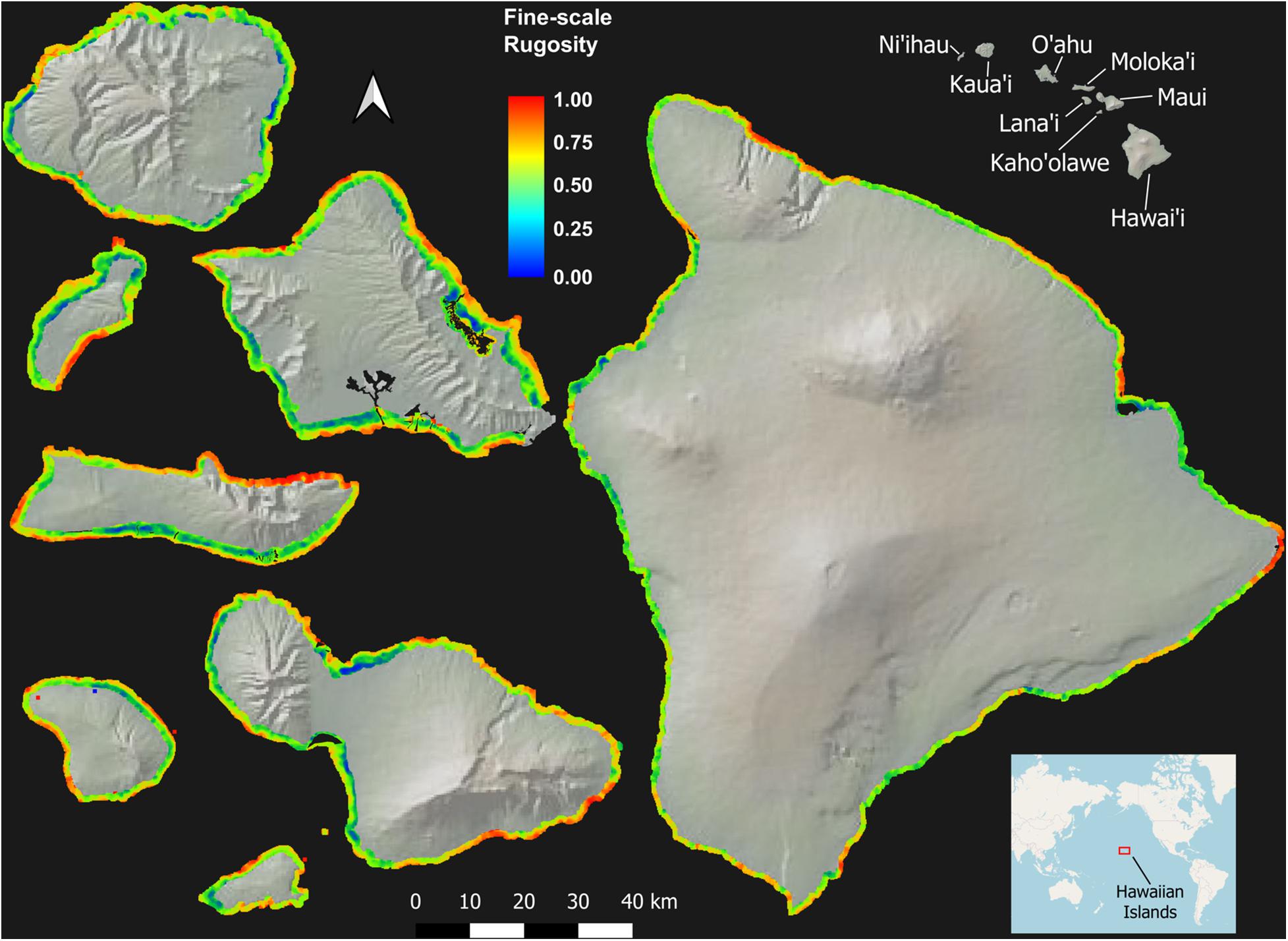
Figure 2. Fine-scale rugosity of the eight Main Hawaiian Islands at 2 m spatial resolution to a depth of 22 m. Values are relative from 0.0 to 1.0. Coarse-scale rugosity is provided in Appendix Figure A1.

TABLE 3

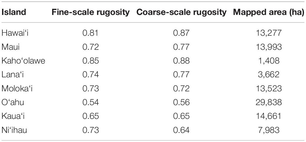
Table 3. Mean fine-scale and coarse-scale rugosity, and the total reef mapping area, of each island in the Main Hawaiian Islands.

Geospatial Variation in Reef Complexity

Despite strong inter-island differences in 3D habitat complexity, any given local reef area displayed a wide range of rugosity values (Figure 3 and Appendix Figure A2). Sandy areas with low rugosity are shown in blue, while highly complex coral and rock reef patches are expressed in yellow to red colors. Relative to shoreline, the location and spatial distribution of high-rugosity benthic surfaces was highly variable, although rugosity can be seen to broadly increase with distance to shore (Figure 3).

FIGURE 3

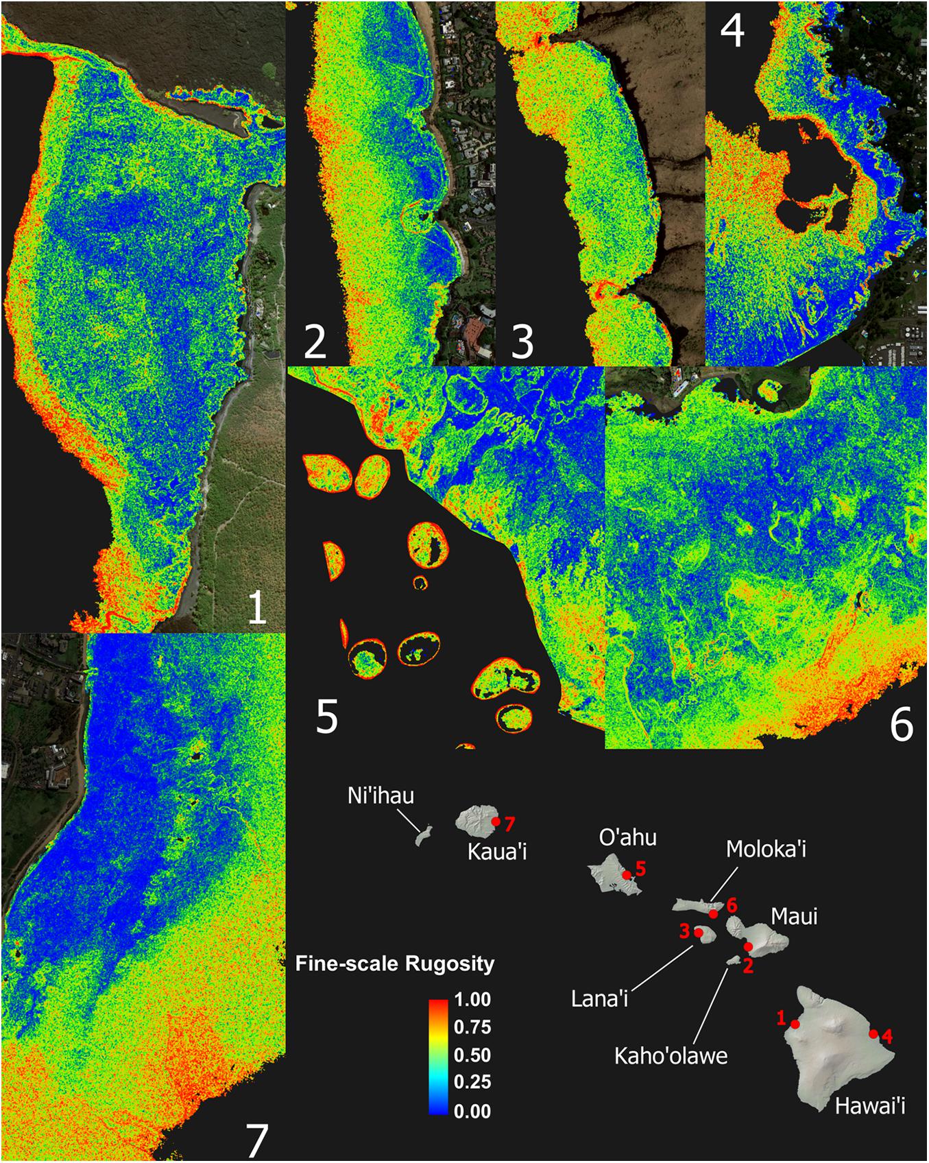
Figure 3. Zoom images from maps shown in Figure 2 demonstrating high spatial frequency variation and pattern in the fine-scale rugosity. These seven example reefs encompass the range of conditions among high-rugosity sites. Coarse-scale rugosity is provided in Appendix Figure A2.

At the individual island level, both fine- and coarse-scale rugosity values were non-normally distributed (Figure 4). Hawai‘i and Kaho‘olawe were highly skewed in the positive direction, indicating the widespread presence of structurally complex benthic surfaces. Field observations indicated that these areas are dominated by rock and/or coral. By contrast, O‘ahu was largely comprised of low-rugosity substrate, with few rocks and coral colonies, and large swaths of sand- and algal-covered surfaces (see Asner et al., 2020b). These contrasting distributions are both an expression of island age, size, and stage as well as how much live coral can be found in each reef ecosystem. Notably, Moloka‘i displayed a bi-modal rugosity distribution, with high values dominating the windward north coast and lower values found along the leeward south coast (Figure 2).

FIGURE 4

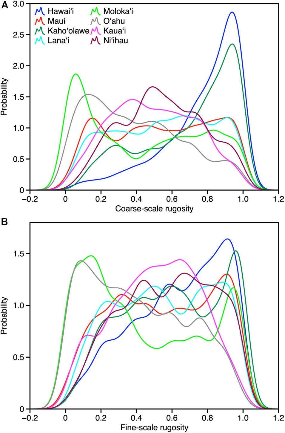
Figure 4. Frequency distributions of (A) coarse-scale and (B) fine-scale rugosity by island.

Reef rugosity showed a highly variable spatial arrangement at intra- and inter-island scales (Figure 5 and Appendix Figure 3). Variogram-range maps reveal that, on geologically older islands such as Ni‘ihau, Kaua‘i and O‘ahu, reef rugosity mostly varied at low spatial frequency, often more than 100 m, indicated by high variogram-range values (Figure 5a and Appendix Figure 3a). However, this background condition was punctuated by reef locations with relatively high spatial frequency changes in rugosity. By contrast, on geologically younger islands such as Hawai‘i, Lana‘i and Maui, low variogram-range values indicated high-frequency variability in rugosity over large tracks of reef. Variogram-sills represent the baseline variation in rugosity between areas on an island that are far enough apart to lack any shared local environmental controls. Again, geologically older islands were largely uniform (Figure 5b and Appendix Figure 3b), whereas younger islands were far more variable. Overall, based on island-level semi-variograms, Lana‘i and Hawai‘i were among the most variable in terms of fine- or coarse-scale rugosity (Figure 5c and Appendix Figure 3c).

FIGURE 5

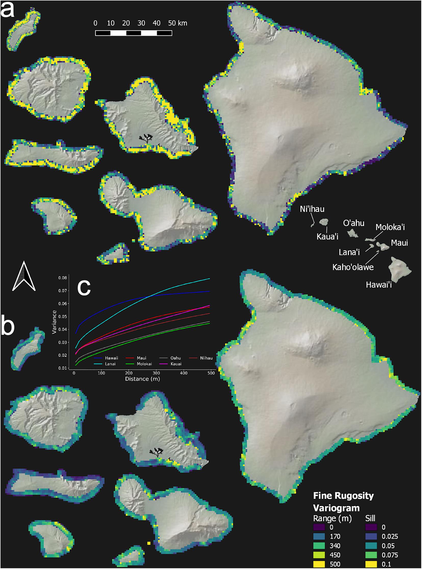
Figure 5. Geospatial variation in fine-scale rugosity for the eight main Hawaiian Islands. Semi-variogram (a) range and (b) sill are shown at the top and bottom, respectively. (c) Island-scale semi-variograms in the inset graph. Coarse-scale rugosity is provided in Appendix Figure A3.

Drivers of Habitat Complexity

Machine learning analyses revealed a heirarchical set of contributors to the spatial variability of fine- and coarse-scale rugosity throughout the MHI (Figure 6). Fine and coarse models accounted for 86 and 73%, respectively, of the overall mapped geospatial variation, indicating that the driver variables used in the model were appropriate in assessing rugosity at both resolutions. Water depth and reef slope exerted the strongest influences on the spatial variation in rugosity as evidenced in model permutation reduction R²-values of up to 0.88 and 0.69, respectively, among all islands combined for fine- and/or coarse-scale rugosity (Figure 6). Secondarily, nearshore development and distance from coast exerted a detectable effect (R² up to 0.31). Other variables such as sea surface temperature, wind speed, total land effluent, and substrate age accounted for far less variation in rugosity (R² < 0.11).

FIGURE 6

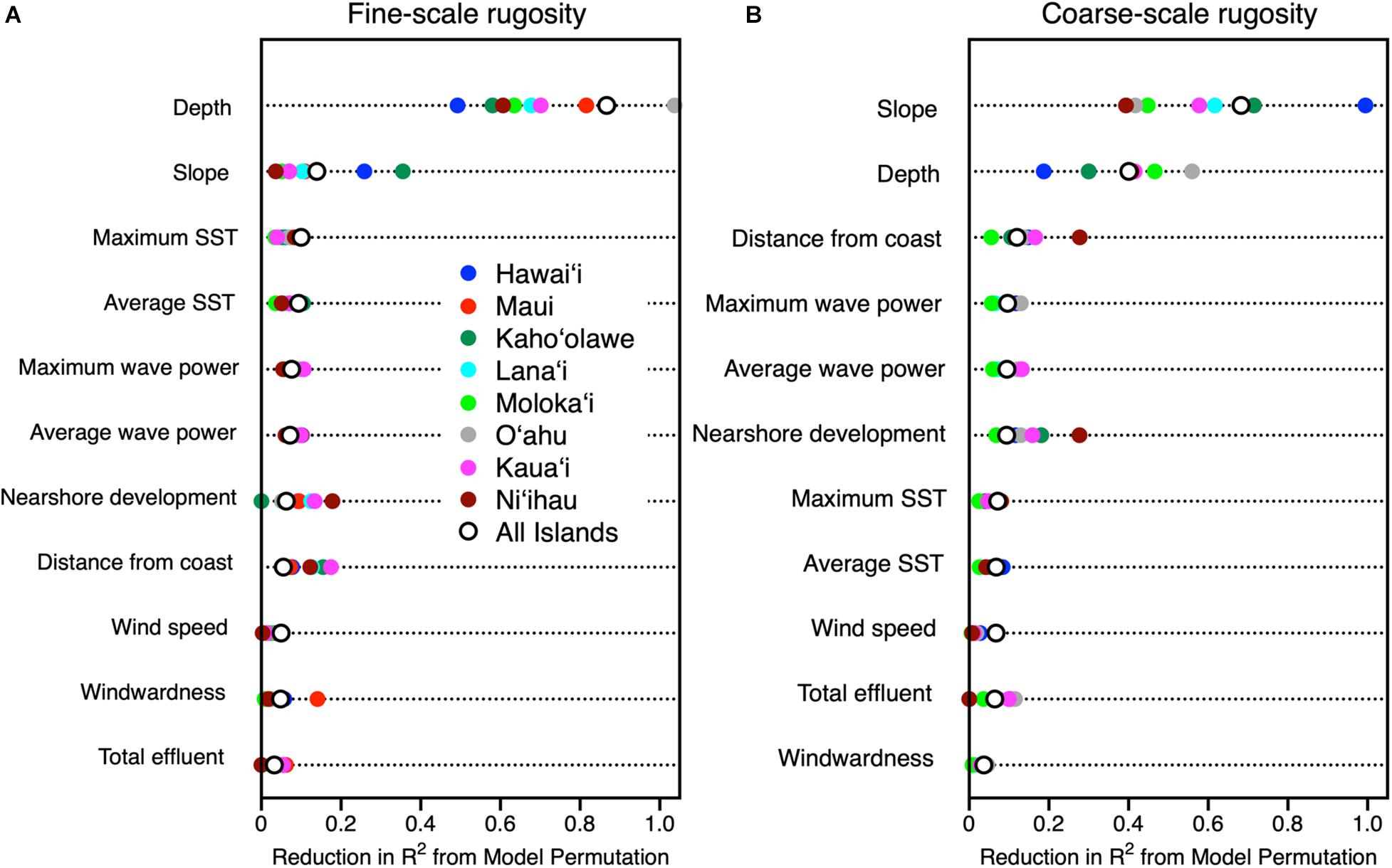
Figure 6. Relative importance of potential contributing variables evaluated using machine learning to drive spatial variation in (A) fine-scale and (B) coarse-scale reef rugosity throughout the eight Main Hawaiian Islands. Colored dots indicate relative importance by island, and open circles indicate relative importance for all islands combined.

There was a wide inter-island range of influence of each major driver on 3D habitat complexity. First, depth was far more important than reef slope in driving fine-scale rugosity, but depth alone ranged in relative importance from low on Hawai‘i to extremely high on O‘ahu (Figure 6a). In contrast, reef slope effect on fine-scale rugosity was minimal on Ni‘ihau but much higher on Hawai‘i. For coarse-scale rugosity, slope exerted the greatest influence on Hawai‘i and the lowest on Ni‘ihau and O‘ahu (Figure 6b). The opposite was true for water depth. Here we note the apparent positive relationship between nearshore development and reef rugosity off Ni‘ihau: Investigation of the mapping data indicated a highly localized spatial correlation between a small area of development and reef presence and rugosity relative to other sandy and cliff-like access points to the coastline.

Examination of model partial dependency indicated that water depth and reef slope had a positive linear relationship with fine-scale rugosity at the scale of the eight MHI (Figure 7). However, coarse-scale rugosity showed an asymptotic relationship with depth and slope (Appendix Figure 4). Moreover, while average fine-scale rugosity across all islands was fairly flat relative to distance to coast and all other factors (Figure 7), distance and wave power did show relationships with coarse-scale rugosity (Appendix Figure 4). We note an especially poor relationship between sea surface temperature and rugosity at either resolution.

FIGURE 7

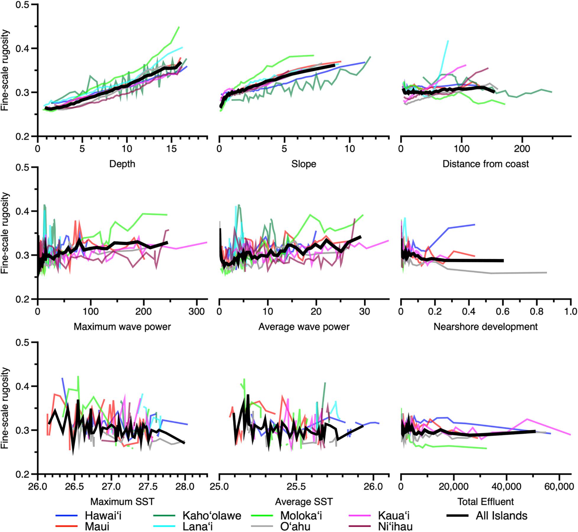
Figure 7. Partial dependence plots indicating the relationship between fine-scale rugosity and the top nine variables presented in Figure 6. Colored lines indicate relationships by island, and thick black lines indicate relationships for all islands combined. Coarse-scale rugosity is provided in Appendix Figure A4.

Discussion

Reef complexity, as indicated by maps of rugosity at 2 and 6 m resolutions, revealed a nested set of 3D habitat patterns across and within the eight MHIs. Coarse-scale rugosity was largely driven by reef slope and secondarily by depth; the opposite was true for fine-scale rugosity (Figure 6). Taken together, these two indicators suggest that geologic stage dominates the broader habitat structure of reefs across the archipelago. Younger islands harbor reefs on steep basaltic slopes, often with rapid drop-offs to extreme depths (Fletcher et al., 2008). During their formation via lava flows, these rock-dominated reefs resemble complex canyon, spire, tube, and spur-and-groove type patterns. As islands age, subside and undergo surficial erosional processes, nearshore shallow (<22 m depth) slopes become smoother (Fletcher et al., 2008), are reduced in rugosity, and show weakening relationships with coarse-scale rugosity (Figure 6).

In contrast to coarse-scale rugosity, the distribution and patterning of fine-scale features were far more driven by water depth than by reef slope (Figure 6), where inter-island differences in rugosity track differently with island age and stage. For example, the youngest island, Hawai‘i, has the steepest nearshore slopes, where depth has relatively little effect on fine-scale rugosity as compared to O‘ahu. For the latter, fine-scale rugosity tracks water depth, largely due to the prevalent role of live coral along forereef locations in the 15+ m range (see Asner et al., 2020b). Shallower inshore areas on O‘ahu are largely devoid of rock or coral needed to drive fine-scale rugosity patterns. It is notable that spatial variation in fine-scale rugosity peaks in the middle-aged islands associated with the conglomerate geologic structure of Maui Nui (Figure 5), comprised of the islands of Maui, Lana‘i, Kaho‘olawe, and Moloka‘i (Price and Elliott-Fisk, 2004). On these islands, reefs undergo large spatially explicit swings in fine-scale rugosity, which we hypothesize to be associated with highly variable coral habitat conditions moderated by substrate availability, currents, depth, and other sub-regional factors (Asner et al., 2020b). Such high-frequency variability in fine-scale rugosity is far less prevalent on older (Kaua‘i, O‘ahu) and younger (Hawai‘i) islands (Figure 5).

Overlain on these geologically driven patterns, there may be an emerging set of 3D habitat conditions associated with nearshore development and other direct human impacts, but the signal remains variable by island (Figure 6). On islands with developed land-based infrastructure like O‘ahu, fine-scale rugosity appears suppressed in areas of nearshore development (Figure 7), perhaps related to the suppression of live coral cover in these locations (Asner et al., 2020b). On other less developed islands like Hawai‘i, fine-scale rugosity was positively related to nearshore development, perhaps because the relationship between land and reef patterns has not yet been sufficiently altered (Wedding et al., 2018). Repeat flights are required to identify areas with changing rugosity for subsequent mitigation actions related to nearshore development.

Beyond the drivers of reef complexity, our rugosity maps have revealed a nested set of patterns ranging in scale from local to archipelago. In a recent study across the MHI, the rugosity maps presented here were a primary determinant of resource fish, herbivore fish, and total fish biomass (Donovan et al., 2020). They also showed that the recovery potential for reef fish was strongly mediated by reef rugosity. These findings amplify both the importance of high-resolution reef complexity mapping and monitoring as well as the way that management can integrate habitat mapping into plans and actions to protect and restore reef fisheries (Nowlis and Friedlander, 2005; Wedding et al., 2008).

Two major limits to our study involve spatial resolution and maximum achieved depth. In our companion study describing the methods and validation for mapping 3D habitat complexity used here, Asner et al. (2020a) found that rugosity maps could be generated at 40–60 cm resolution, thereby revealing the location of smaller coral colonies and rock outcrops. These smaller features may be key to understanding a host of other reef patterns and processes such as fish and invertebrate dynamics, coral larval settlement, and disease (Hata et al., 2017; Eggertsen et al., 2020). The current study cannot resolve these ultra-fine rugosity issues due to the practicalities of mapping an entire archipelago at high altitude and thus lower (2 m) spatial resolution.

Our maximum achieved mapping depth was 22 m (72 fsw). While much of the biological diversity of Hawaiian reefs is contained within our mappable depth range, critically important habitat in the lower euphotic and mesophotic zones are missed by our current approach (Rooney et al., 2010; Baldwin et al., 2018). While we continue to push the limits of spectroscopy-based depth and rugosity mapping, with some indications of 30 m penetrability in clear waters (G.P. Asner, unpub. data), this is not likely to become operational in the near future due to the limits of solar photon flux at such depths paired with limits of our high-fidelity imaging spectrometers. While these current spectrometer-based approaches are limited to a very few manned aircraft platforms, the technology is downsizing and could become UAV (drone) based in the coming years. Additionally, these types of high-fidelity spectrometers are being prepared for low Earth orbit, such as the NASA Surface Biology and Geology mission (Schneider et al., 2019). Although the planned spatial resolution of 30 m will remain coarse for reef applications, the quality of the spectroscopic measurement will be analogous to the airborne capability today, perhaps allowing for coarse-scale rugosity mapping worldwide with the ecological fidelity proven here at an archipelago scale.

We found that water depth and reef slope are dominant drivers of both fine- and coarse-scale rugosity, where the greatest variation in rugosity occurred on middle-aged islands (e.g., Maui) in comparison to young and older islands (e.g., Hawai‘i, Kaua‘i). Nearshore development is an emerging secondary driver of decreasing rugosity, for example on O‘ahu, the most highly developed island. Our rugosity maps are a tool that can be used by fisheries management and reef practitioners to prioritize areas for conservation and to design marine managed areas for greater resilience and recovery potential.

Data Availability Statement

The datasets presented in this study can be found in online repositories. The names of the repository/repositories and accession number(s) can be found in Asner et al. (2020c).

Author Contributions

GA conceived and funded the study, collected the data, provided the analysis, and wrote the manuscript. NV and JH collected the data, provided the analysis, and contributed to the writing of the manuscript. SF, ES, and RM provided the analysis and contributed to the writing of the manuscript. All authors contributed to the article and approved the submitted version.

Funding

This study was supported by the Lenfest Ocean Program and The Battery Foundation. The Global Airborne Observatory is made possible with support of private foundations, visionary individuals, and Arizona State University.

Conflict of Interest

The authors declare that the research was conducted in the absence of any commercial or financial relationships that could be construed as a potential conflict of interest.

Supplementary Material

The Supplementary Material for this article can be found online at: https://www.frontiersin.org/articles/10.3389/fmars.2021.631842/full#supplementary-material

References

Alvarez-Filip, L., Dulvy, N. K., Gill, J. A., Côté, I. M., and Watkinson, A. R. (2009). Flattening of Caribbean coral reefs: region-wide declines in architectural complexity. Proc. R. Soc. B 276, 3019–3025. doi: 10.1098/rspb.2009.0339

PubMed Abstract | CrossRef Full Text | Google Scholar

Asner, G. P., Knapp, D. E., Boardman, J., Green, R. O., Kennedy-Bowdoin, T., Eastwood, M., et al. (2012). Carnegie Airborne Observatory-2: Increasing science data dimensionality via high-fidelity multi-sensor fusion. Remote Sens. Environ. 124, 454–465. doi: 10.1016/j.rse.2012.06.012

CrossRef Full Text | Google Scholar

Asner, G. P., Vaughn, N. R., Balzotti, C., Brodrick, P. G., and Heckler, J. (2020a). High-resolution reef bathymetry and coral habitat complexity from airborne imaging spectroscopy. Remote Sens. 12:310. doi: 10.3390/rs12020310

CrossRef Full Text | Google Scholar

Asner, G. P., Vaughn, N. R., Heckler, J., Knapp, D. E., Balzotti, C., Shafron, E., et al. (2020b). Large-scale mapping of live corals to guide reef conservation. Proc. Natl. Acad. Sci. 117, 33711–33718. doi: 10.1073/pnas.2017628117

PubMed Abstract | CrossRef Full Text | Google Scholar

Asner, G. P., Vaughn, N. R., and Heckler, J. (2020c). Global airborne observatory: hawaiian islands reef rugosity 2019+2020 (Version 1.0) [Data set]. Zenodo. doi: 10.5281/zenodo.4294332

CrossRef Full Text | Google Scholar

Aston, E. A., Williams, G. J., Green, J. A. M., Davies, A. J., Wedding, L. M., Gove, J. M., et al. (2019). Scale-dependent spatial patterns in benthic communities around a tropical island seascape. Ecography 42, 578–590. doi: 10.1111/ecog.04097

CrossRef Full Text | Google Scholar

Baldwin, C. C., Tornabene, L., and Robertson, D. R. (2018). Below the mesophotic. Sci. Reports 8:4920.

Google Scholar

Bezanson, J., Karpinski, S., Shah, V. B., and Edelman, A. (2012). Julia: A Fast Dynamic Language for Technical Computing. ArXiv 2012, 1209.51451.

Google Scholar

Breiman, L. (2001). Random forests. Machine Learn. 45, 5–32.

Google Scholar

Burns, J., Delparte, D., Gates, R., and Takabayashi, M. (2015). Integrating structure-from-motion photogrammetry with geospatial software as a novel technique for quantifying 3D ecological characteristics of coral reefs. PeerJ. 3:e1077. doi: 10.7717/peerj.1077

PubMed Abstract | CrossRef Full Text | Google Scholar

Center for International Earth Science Information Network-Ciesin, C. U. (2018). “Gridded Population of the World, Version 4 (GPWv4): Population Count,” in NASA Socioeconomic Data and Applications Center (SEDAC), (Palisades, NY: Columbia University).

Google Scholar

Cinner, J. E., Mcclanahan, T. R., Daw, T. M., Graham, N. A. J., Maina, J., Wilson, S. K., et al. (2009). Linking social and ecological systems to sustain coral reef fisheries. Curr. Biol. 19, 206–212. doi: 10.1016/j.cub.2008.11.055

PubMed Abstract | CrossRef Full Text | Google Scholar

Donovan, M. K., Counsell, C. W. W., Lecky, J., and Donahue, M. J. (2020). Estimating indicators and reference points in support of effectively managing nearshore marine resources in Hawai‘i, Report by Hawai: Monitoring and Reporting Collaborative.

Google Scholar

Eggertsen, M., Chacin, D. H., Van Lier, J., Eggertsen, L., Fulton, C. J., Wilson, S., et al. (2020). Seascape configuration and fine-scale habitat complexity shape parrotfish distribution and function across a coral reef lagoon. Diversity 12:391. doi: 10.3390/d12100391

CrossRef Full Text | Google Scholar

Engelen, A. H., Åberg, P., Olsen, J. L., Stam, W. T., and Breeman, A. M. (2005). Effects of wave exposure and depth on biomass, density and fertility of the fucoid seaweed Sargassum polyceratium (Phaeophyta. Sargassaceae). Eur. J. Phycol. 40, 149–158. doi: 10.1080/09670260500109210

CrossRef Full Text | Google Scholar

Figueira, W., Ferrari, R., Weatherby, E., Porter, A., Hawes, S., and Byrne, M. (2015). Accuracy and precision of habitat structural complexity metrics derived from underwater photogrammetry. Remote Sens. 7, 16883–16900. doi: 10.3390/rs71215859

CrossRef Full Text | Google Scholar

Fletcher, C. H., Bochicchio, C., Conger, C. L., Engels, M. S., Feirstein, E. J., Frazer, N., et al. (2008). “Geology of Hawaii Reefs,” in Coral Reefs of the USA, eds B. M. Riegl and R. E. Dodge (Dordrecht: Springer Netherlands), 435–487.

Google Scholar

Gao, B.-C., and Goetz, A. F. H. (1990). Column atmospheric water vapor and vegetation liquid water retrievals from airborne imaging spectrometer data. J. Geophys. Res. 95, 3549–3564. doi: 10.1029/jd095id04p03549

CrossRef Full Text | Google Scholar

Gove, J., Williams, G., Mcmanus, M., Clark, S., Ehses, J. S., and Wedding, L. (2015). Coral reef benthic regimes exhibit non-linear threshold responses to natural physical drivers. Mar. Ecol. Prog. Series 522, 33–48. doi: 10.3354/meps11118

CrossRef Full Text | Google Scholar

Graham, N. A. J., and Nash, K. L. (2012). The importance of structural complexity in coral reef ecosystems. Coral Reefs 32, 315–326. doi: 10.1007/s00338-012-0984-y

CrossRef Full Text | Google Scholar

Graham, N. A. J., Wilson, S. K., Pratchett, M. S., Polunin, N. V. C., and Spalding, M. D. (2009). Coral mortality versus structural collapse as drivers of corallivorous butterflyfish decline. Biodiver. Conserv. 18, 3325–3336. doi: 10.1007/s10531-009-9633-3

CrossRef Full Text | Google Scholar

Gratwicke, B., and Speight, M. R. (2005). The relationship between fish species richness, abundance and habitat complexity in a range of shallow tropical marine habitats. J. Fish Biol. 66, 650–667. doi: 10.1111/j.0022-1112.2005.00629.x

CrossRef Full Text | Google Scholar

Grigg, R. W. (1998). Holocene coral reef accretion in Hawaii: a function of wave exposure and sea level history. Coral Reefs 17, 263–272. doi: 10.1007/s003380050127

CrossRef Full Text | Google Scholar

Grober-Dunsmore, R., Frazer, T. K., Lindberg, W. J., and Beets, J. (2007). Reef fish and habitat relationships in a Caribbean seascape: the importance of reef context. Coral Reefs 26, 201–216. doi: 10.1007/s00338-006-0180-z

CrossRef Full Text | Google Scholar

Harborne, A. R., Mumby, P. J., and Ferrari, R. (2012). The effectiveness of different meso-scale rugosity metrics for predicting intra-habitat variation in coral-reef fish assemblages. Environ. Biol. Fishes 94, 431–442. doi: 10.1007/s10641-011-9956-2

CrossRef Full Text | Google Scholar

Harborne, A. R., Mumby, P. J., Żychaluk, K., Hedley, J. D., and Blackwell, P. G. (2006). Modeling the beta diversity of coral reefs. Ecology 87, 2871–2881.

Google Scholar

Hata, T., Madin, J. S., Cumbo, V. R., Denny, M., Figueiredo, J., Harii, S., et al. (2017). Coral larvae are poor swimmers and require fine-scale reef structure to settle. Sci. Reports 7:2249.

Google Scholar

Hoffimann, J. (2018). GeoStats.jl – High-performance geostatistics in Julia. J. Open Source Software 3:692. doi: 10.21105/joss.00692

CrossRef Full Text | Google Scholar

Ignatov, A. (2010). GOES-R Advanced Baseline Imager (ABI) algorithm theoretical basis document for sea surface temperature. Washington, D.C: NOAA NESDIS Center for Satellite Applications and Research.

Google Scholar

Jenness, J. S. (2004). Calculating landscape surface area from digital elevation models. Wildlife Soc. Bulletin 32, 829–839. doi: 10.2193/0091-7648(2004)032[0829:clsafd]2.0.co;2

CrossRef Full Text | Google Scholar

Jennings, S., Boullé, D. P., and Polunin, N. V. C. (1996). Habitat correlates of the distribution and biomass of Seychelles’ reef fishes. Env. Biol. Fishes 46, 15–25. doi: 10.1007/bf00001693

CrossRef Full Text | Google Scholar

Lechene, M. A. A., Haberstroh, A. J., Byrne, M., Figueira, W., and Ferrari, R. (2019). Optimising sampling strategies in coral reefs using large-area mosaics. Remote Sens. 11:2907. doi: 10.3390/rs11242907

CrossRef Full Text | Google Scholar

Li, N., Cheung, K. F., Stopa, J. E., Hsiao, F., Chen, Y.-L., Vega, L., et al. (2016). Thirty-four years of Hawaii wave hindcast from downscaling of climate forecast system reanalysis. Ocean Model. 100, 78–95. doi: 10.1016/j.ocemod.2016.02.001

CrossRef Full Text | Google Scholar

Madin, J. S., Baird, A. H., Dornelas, M., and Connolly, S. R. (2014). Mechanical vulnerability explains size-dependent mortality of reef corals. Ecol. Lett. 17, 1008–1015. doi: 10.1111/ele.12306

PubMed Abstract | CrossRef Full Text | Google Scholar

Moravec, H., and Elfes, A. (1985). “High resolution maps from wide angle sonar,” in Proceedings of the 1985 IEEE International Conference on Robotics and Automation. Missouri. 116–121.

Google Scholar

Mumby, P. J., Skirving, W., Strong, A. E., Hardy, J. T., Ledrew, E. F., Hochberg, E. J., et al. (2004). Remote sensing of coral reefs and their physical environment. Mar. Pollut. Bull. 48, 219–228.

Google Scholar

Neall, V. E., and Trewick, S. A. (2008). The age and origin of the Pacific islands: a geological overview. Philosoph. Transac. R. Soc. B 363, 3293–3308. doi: 10.1098/rstb.2008.0119

PubMed Abstract | CrossRef Full Text | Google Scholar

Nowlis, J. S., and Friedlander, A. (2005). Marine reserve function and design for fisheries management. Washington, D.C: Island Press.

Google Scholar

Pedregosa, F., Varoquaux, G., Gramfort, A., Michel, V., Thirion, B., Grisel, O., et al. (2011). Scikit-learn: Machine learning in Python. J. Machine Learn. Res. 12, 2825–2830.

Google Scholar

Price, J. P., and Elliott-Fisk, D. (2004). Topographic History of the Maui Nui Complex, Hawai‘i, and Its Implications for Biogeography. Pacific Sci. 58, 27–45. doi: 10.1353/psc.2004.0008

CrossRef Full Text | Google Scholar

Purkis, S. J., Graham, N. A. J., and Riegl, B. M. (2008). Predictability of reef fish diversity and abundance using remote sensing data in Diego Garcia (Chagos Archipelago). Coral Reefs 27, 167–178. doi: 10.1007/s00338-007-0306-y

CrossRef Full Text | Google Scholar

Risk, M. J. (1972). Fish diversity on a coral reef in the Virgin Islands. Atoll Res. Bull 153, 1–7. doi: 10.5479/si.00775630.153.1

CrossRef Full Text | Google Scholar

Rogers, A., Blanchard, J., and Mumby, P. (2014). Vulnerability of Coral Reef Fisheries to a Loss of Structural Complexity. Curr. Biol. 24, 1000–1005. doi: 10.1016/j.cub.2014.03.026

PubMed Abstract | CrossRef Full Text | Google Scholar

Rooney, J., Donham, E., Montgomery, A., Spalding, H., Parrish, F., Boland, R., et al. (2010). Mesophotic coral ecosystems in the Hawaiian Archipelago. Coral Reefs 29, 361–367. doi: 10.1007/s00338-010-0596-3

CrossRef Full Text | Google Scholar

Schneider, F. D., Ferraz, A., and Schimel, D. (2019). Watching Earth’s interconnected systems at work. Eos, 100. doi: 10.1029/2019EO136205

CrossRef Full Text | Google Scholar

Sebens, K. P. (1991). “Habitat structure and community dynamics in marine benthic systems,” in Habitat Structure: The physical arrangement of objects in space, eds S. S. Bell, E. D. Mccoy, and H. R. Mushinsky (Dordrecht: Springer Netherlands), 211–234. doi: 10.1007/978-94-011-3076-9_11

CrossRef Full Text | Google Scholar

Storlazzi, C. D., Brown, E. K., Field, M. E., Rodgers, K., and Jokiel, P. L. (2005). A model for wave control on coral breakage and species distribution in the Hawaiian Islands. Coral Reefs 24, 43–55. doi: 10.1007/s00338-004-0430-x

CrossRef Full Text | Google Scholar

Thompson, D. R., Hochberg, E. J., Asner, G. P., Green, R. O., Knapp, D. E., Gao, B.-C., et al. (2017). Airborne mapping of benthic reflectance spectra with Bayesian linear mixtures. Remote Sens. Environ. 200, 18–30. doi: 10.1016/j.rse.2017.07.030

CrossRef Full Text | Google Scholar

Wedding, L. M., Friedlander, A. M., Mcgranaghan, M., Yost, R. S., and Monaco, M. E. (2008). Using bathymetric lidar to define nearshore benthic habitat complexity: Implications for management of reef fish assemblages in Hawaii. Remote Sens. Environ. 112, 4159–4165. doi: 10.1016/j.rse.2008.01.025

CrossRef Full Text | Google Scholar

Wedding, L. M., Lecky, J., Gove, J. M., Walecka, H. R., Donovan, M. K., Williams, G. J., et al. (2018). Advancing the integration of spatial data to map human and natural drivers on coral reefs. PLoS One 13:e0204760. doi: 10.1371/journal.pone.0204760

PubMed Abstract | CrossRef Full Text | Google Scholar

Williams, G. J., Gove, J. M., Eynaud, Y., Zgliczynski, B. J., and Sandin, S. A. (2015). Local human impacts decouple natural biophysical relationships on Pacific coral reefs. Ecography 38, 751–761. doi: 10.1111/ecog.01353

CrossRef Full Text | Google Scholar