Optimal Spatiotemporal Scales to Aggregate Satellite Ocean Color Data for Nearshore Reefs and Tropical Coastal Waters: Two Case Studies

Introduction

Good water quality is essential for healthy coastal ecosystems and recent increases in land-based sources of pollution (LBSP) threaten the persistence of many ecologically important nearshore species. Water quality is defined by several factors such as the turbidity, productivity, salinity, amount of sediment, nutrients, dissolved oxygen, and other pollutants present within the water column. Human expansion has dramatically increased coastal LBSP and negatively affected water quality in nearshore environments impacting most of the world’s coral reefs (Fabricius, 2005; Sheridan et al., 2014; Otaño-Cruz et al., 2017). Climate change, sea level rise, and the increasing frequency of hurricanes and other natural disasters exacerbate the impacts of anthropogenic LBSP through increased runoff, coastal erosion, and sediment resuspension (Nearing et al., 2005). Excess sediment and nutrients that lead to eutrophication can degrade coastal ecosystem health by limiting light availability necessary for photosynthetic organisms and disrupting oligotrophic ecosystems.

Coral reef ecosystems are particularly sensitive to changes in water quality. There have been substantial ecosystem declines in reef regions around the world (Pandolfi et al., 2003; Burke et al., 2011; Hughes et al., 2018), and increased sediment and nutrient loads indirectly threaten one-third of remaining reef-building corals by disrupting reef biological processes and increasing coral disease (Rogers, 1990; Carpenter et al., 2008; Thompson et al., 2014; UNEP, 2017). In tropical nearshore waters, structure-building corals provide the underlying habitat that supports the high biodiversity of coral reefs and the many ecosystem services they provide. Tropical corals live close to their upper light and temperature tolerance thresholds (Rodolfo-Metalpa et al., 2014) and, as sessile organisms, they are highly sensitive to changes in water quality, which modifies temperature, light, and availability of both beneficial and detrimental nutrients (Lesser et al., 2009). Turbid water from sedimentation, nutrient input, and other LBSP can impair reef growth and lead to degradation of existing reefs. For example, suspended sediment decreases the light available to zooxanthellate corals for photosynthesis, and deposited sediment limits coral recruitment and is energetically costly for corals to remove (Fabricius, 2005; Weber et al., 2012). Sediment resulting from coastal dredging has similar deleterious impacts and may also act as a catalyst for the spread of coral disease (Pollock et al., 2014). High nutrient input from terrestrial runoff can cause eutrophication that leads to phytoplankton and algae blooms, further reducing light availability.

Quantifying water quality in coastal ecosystems has largely depended on highly accurate but small-scale in situ measurements and less accurate but larger-scale complementary data from remotely sensed ocean color instruments. While in situ water quality measurements can be highly accurate, they are time-consuming, labor-intensive, and often expensive and therefore difficult to collect over regional scales (Duan et al., 2013). These measurement methods are also limited in their ability to track the spatial and temporal variability in water quality in large water bodies (Gholizadeh et al., 2016). Weather conditions may also inhibit in situ measurement collection, and in the case of Hurricane Maria in Puerto Rico, destroy existing monitoring infrastructure (Hernández et al., 2020). As such, previous studies have used remotely sensed ocean color data to estimate water quality parameters in coastal environments (Thompson et al., 2014; Gholizadeh et al., 2016; Hernández et al., 2020). These data provide complementary information to in situ measurements and are useful for estimating water quality parameters over broad areas.

One such satellite-derived parameter is the diffuse attenuation coefficient at 490 nm, K_d(490) (Lee et al., 2005; Morel et al., 2007; Wang et al., 2009). K_d(490) is an apparent optical property that acts as a proxy for turbidity in the water column and can be used to quantify light availability for benthic ecosystems such as coral reefs (Kirk, 2011; Hernández et al., 2020). Two limitations of ocean color algorithms for remotely sensed water quality observations over coral reefs are the frequent presence of clouds along tropical shorelines (Gholizadeh et al., 2016), and the confounding of water column measurements due to bottom reflectance in clear, shallow water (Reichstetter et al., 2015). The presence of clouds increases when using instruments aboard an afternoon-overpass satellite like Suomi-National Polar-orbiting Partnership (NPP) or NOAA-20. Optically shallow waters can confound algorithms due to bottom reflectance, interfering with measurement of near-coast turbidity (McKinna and Werdell, 2018). Waters are considered optically shallow when the physical depth of the measurement location is less than the depth to which penetrating light would be optically significant (Bailey and Werdell, 2006). While previous work to improve algorithms for optically shallow waters and minimize bottom reflectance issues has been tested in Florida and the Gulf of Mexico (Barnes et al., 2013; Hu et al., 2014; Barnes et al., 2018), these algorithms have not been implemented operationally by NOAA or NASA. In addition to cloud presence and bottom reflectance, the practice of using only the highest quality satellite data affects the quantity of data available due to quality control flags, which account for perturbations such as stray light and sun glint, further removing data from consideration (Feng and Hu, 2015; Hu et al., 2020). Multi-satellite approaches can reduce data gaps, but are limited by the insufficient frequency of polar-orbiting satellite overpasses and prove difficult to implement due to instrument and algorithm differences across sensors (Sathyendranath et al., 2019). NOAA has been using Data Interpolating Empirical Orthogonal Functions (DINEOF) on single-sensor and merged-sensor datasets to successfully fill gaps and capture meso- and large-scale ocean features, highlighting the need for gapless datasets, but this method has not been tested at resolutions less than 9 km (Liu and Wang, 2018, 2019). Aggregating data from one instrument over space and time scales is routinely done by NOAA and NASA to produce a more complete time series (e.g, 3-, 8-days, monthly, and seasonal averages at 4 and 9 km globally). However, aggregating over space and time has the potential to smooth out small-scale features that are of interest to coastal managers. Globally standardized aggregation scales may not be optimal for all locations due to localized small-scale episodic changes in water quality.

This study investigated the relationship of in situ data with space and time aggregations of corresponding satellite K_d(490) to determine how well satellite data describe environmental variability at scales applicable to coral reefs. Data from the Visible Infrared Imaging Radiometer Suite (VIIRS) instrument (nominal spatial resolution of 750 m) aboard the Suomi-NPP satellite at several coral reef locations in Maui, Hawai‘i and southwestern Puerto Rico were compared with in situ measurements of K_d(490) and turbidity. The performance of aggregated satellite data was assessed in terms of how well the data correspond to in situ data to describe acute and chronic water quality, both of which are ecologically important to coral reefs. Improving the data availability of satellite-derived water quality while maintaining a robust relationship with in situ measurements will enhance the utility and reliability of satellite data for use in the monitoring and management of events that affect water quality, as well as understanding of the ecological implications of such events.

Materials and Methods

This study compares the globally available satellite remote sensing dataset from VIIRS with two types of in situ data in Maui, Hawai‘i and Puerto Rico (Figure 1). In Maui, the focus is on spatial dynamics and aggregated VIIRS data are compared with (i) in situ nearshore optical data collected at 11 sites over three days and (ii) in situ onshore turbidity measurements collected at 51 sites over three years. In Puerto Rico, the focus is on temporal dynamics and aggregated VIIRS data are compared with a four-year in situ time series of nearshore optical data at a single location. The following sections describe the data sources and collection methods in more detail.

FIGURE 1

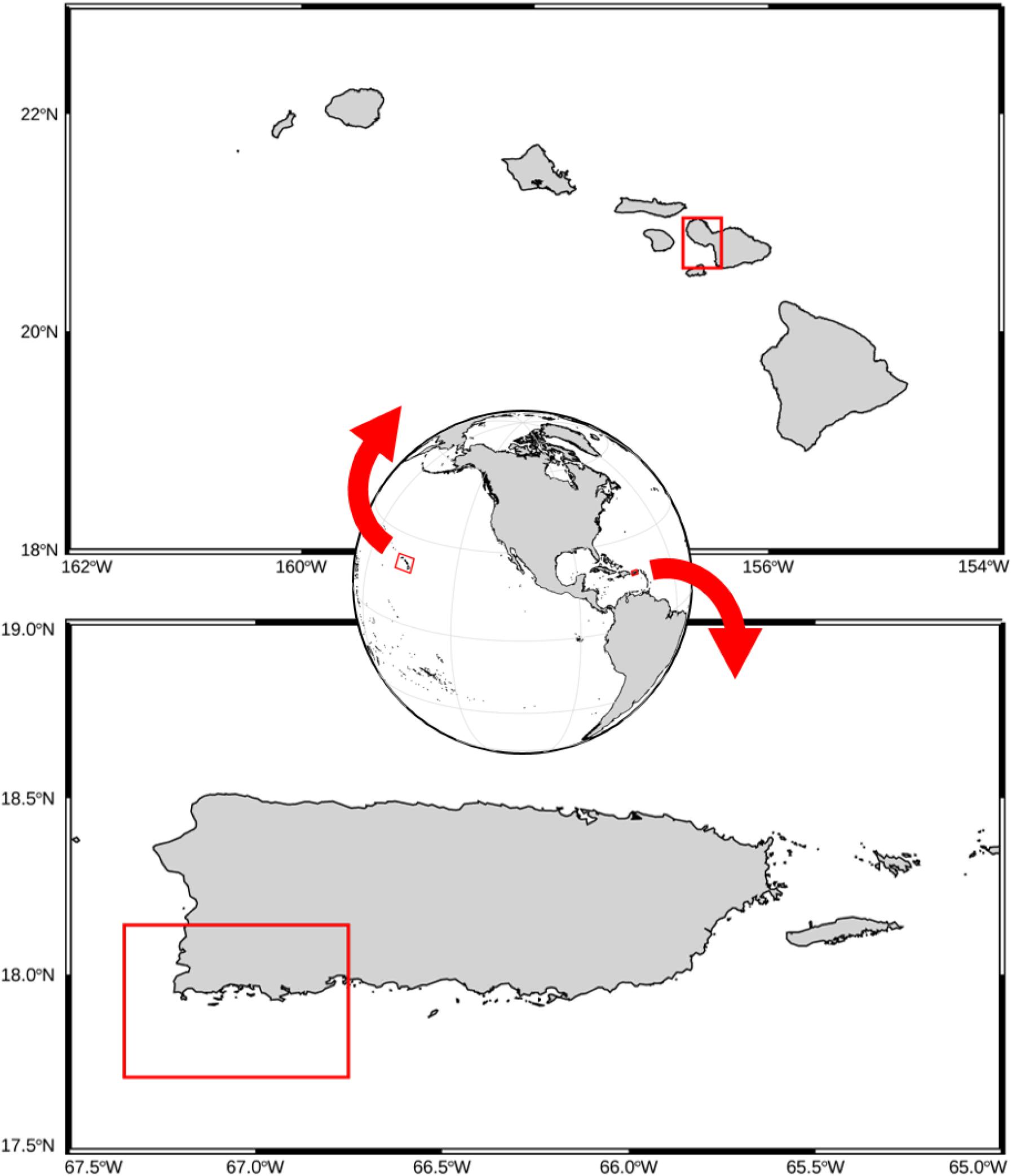
Figure 1. Location of study areas (red boxes) in West Maui, Hawai‘i (top) and southwestern Puerto Rico (bottom).

Nearshore Optical Data Collection—Maui and Puerto Rico

Nearshore optical data in Maui and Puerto Rico were collected using a Sea-Bird Scientific HyperPro II optical profiler (Satlantic) in free-falling mode over the side of a boat, while avoiding ship-shadowing errors (Mueller et al., 2003; Ondrusek et al., 2012). The raw instrument data were processed in Satlantic Prosoft software (v8.0) with calibrated reference data to obtain the attenuation coefficient of downward irradiance at 490 nm, K_d(490) (Lee et al., 2013; Wei et al., 2016). The Maui data consisted of 11 measurements taken at different nearshore sites covering a broad spatial domain (∼17 km²) during November 26 and 28, 2018 (Figure 2). Nine of the nearshore sites in Maui were ∼750 m off the coast (one satellite pixel) and two were more than 750 m off the coast. The Puerto Rico data consisted of 22 measurements taken at one site in the La Parguera Natural Reserve during 2016–2019 (Figure 3). The site in Puerto Rico was more than 750 m off the coast, but within the shelf break. At each measurement site (across both study locations), three instrument casts were taken and collectively used to determine the attenuation coefficient (Supplementary Figure 1). In Maui, four sites can be considered optically shallow at the time of measurement using a conservative measure of apparent optical depth (AOD = 1.3/K_d; Bailey and Werdell, 2006); everywhere else the waters were optically deep (i.e., the apparent optical depth less than the physical depth; Supplementary Table 1).

FIGURE 2

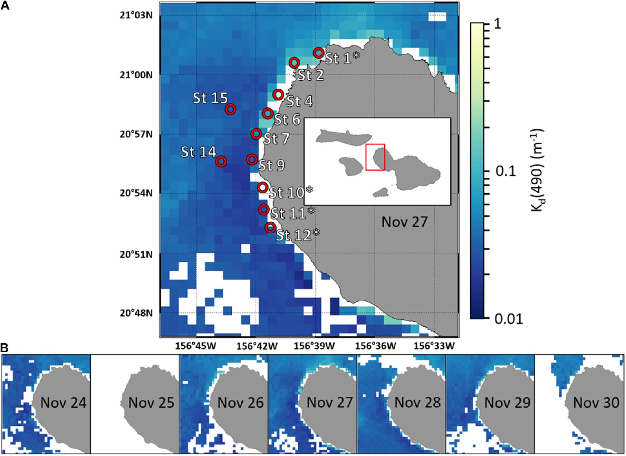
Figure 2. Maps of VIIRS K_d(490) for West Maui, HI for (A) November 27, 2018 (750 m pixel resolution). White areas are missing data due to cloud cover or flagged due to poor quality. The red circles show the locations where 11 in situ optical data measurements were taken on November 26 or November 28, 2018 using a Sea-Bird Scientific HyperPro II; and (B) the 7-days period from November 24–30, 2018, illustrating the variability in satellite data coverage. Sites marked with a white asterisk were considered optically shallow during the time of measurement (see Supplementary Table 1).

FIGURE 3

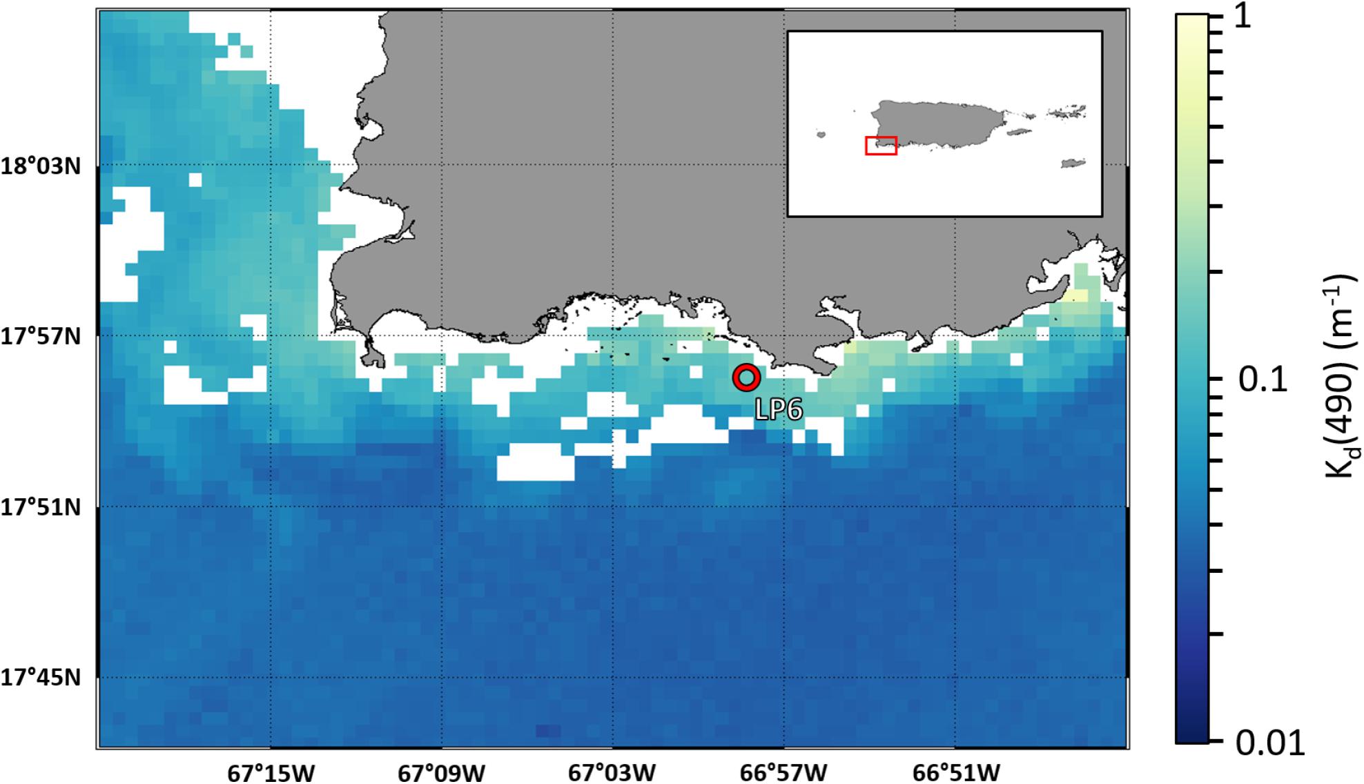
Figure 3. Map of VIIRS K_d(490) for southwestern Puerto Rico for November 9, 2016 (750 m pixel resolution). White areas are missing data due to cloud cover or flagged due to poor quality. The red circle shows the location where 22 in situ optical data measurements were taken between 2016 and 2019 using a Sea-Bird Scientific HyperPro II.

Onshore Turbidity Data Collection—Maui

Onshore turbidity data were collected using a Hach 2100Q turbidimeter in < 1 m deep water along the west and south Maui coasts at 51 fixed sites (±3 m of accuracy) that are representative of water quality types along the stretch of coastline. Data were collected between June 15, 2016 and June 15, 2019 (Figure 4). Sites were chosen to be adjacent to but not directly in front of surface water discharges. The turbidimeter reports measurements in Nephelometric Turbidity Units (NTU). These measurements are an ongoing effort in collaboration with Hui o Ka Wai Ola, a local water quality-monitoring group (http://huiokawaiola.com), and the Hawai‘i State Department of Health. The number of NTU measurements and dates they were collected varies between sites (Supplementary Table 2).

FIGURE 4

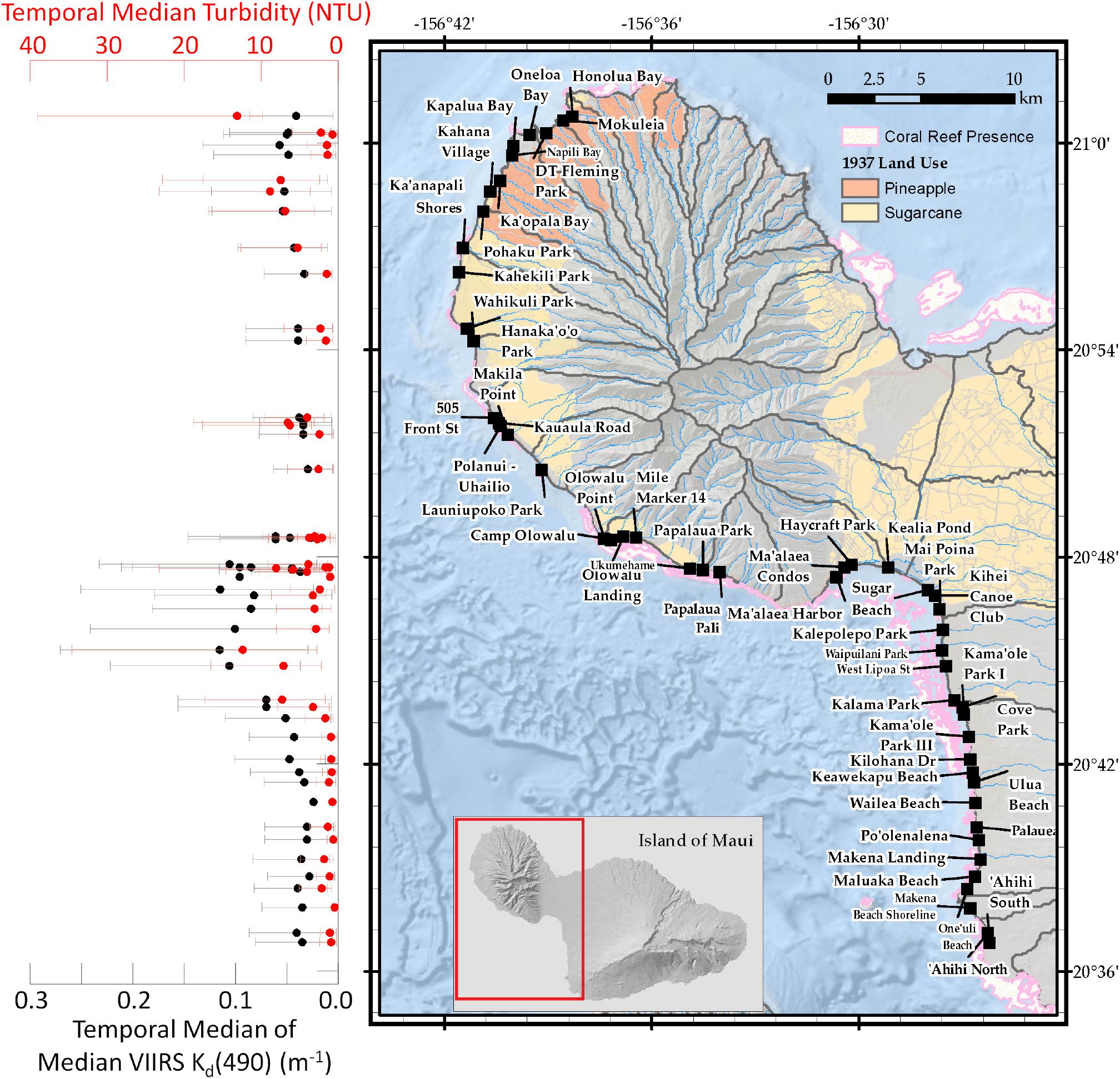
Figure 4. (Left) Temporal median of the time series of (red, upper axis) in situ turbidity (NTU) and (black, lower axis) spatiotemporal (median of 5-pixels, 7-days cube) satellite K_d(490) (m^–1) for each site by latitude in West Maui, HI. In situ turbidity measurements were taken using a Hach 2100Q turbidimeter. Data were included in the analysis only when in situ observations and satellite observations (in a 5-pixels, 7-days cube) were both available. Whiskers represent the 1st and 3rd quartiles of underlying time series data for each dataset, respectively. (Right) Map of collection sites along the West Maui coast. The 1937 land use layer shows areas historically used for pineapple (orange) and sugarcane (yellow) production. The pink with yellow pattern area shows coral reef presence along the coast.

VIIRS K_d(490) Ocean Color Data—Maui and Puerto Rico

Ocean color data are from the Visible Infrared Imaging Radiometer Suite (VIIRS) sensor aboard the Suomi-NPP satellite. Data are available for download as science-quality, Level-2 swaths (nominal resolution 750 m) from NOAA CoastWatch (NOAA, 2021). The NOAA Center for Satellite Applications and Research Ocean Color Team has been routinely producing ocean color products for VIIRS since its launch on October 28, 2011 using the NOAA Multi-Sensor Level-1 to Level-2 Processing System (NOAA-MSL12 v1.2) (Wang et al., 2009, 2017). The algorithms that produce K_d(490) are a weighted combination of clear open ocean and turbid water algorithms (Wang et al., 2017; Eqs. 12–16). Algorithm validation was undertaken using the predecessor to VIIRS (Moderate Resolution Imaging Spectroradiometer, MODIS) for which the mean ratio of satellite to in situ K_d(490) was 1.037 (Wang et al., 2009). Subsequent comparison of VIIRS and MODIS data demonstrated consistent K_d(490) values (Wang et al., 2017). For this study, Level-2 swath data for Hawai‘i and Puerto Rico were binned to a geographic projection with pixel size of 0.0075 degrees (∼750 m) using CoastWatch Utilities software (v3.6.0). VIIRS overpasses occur once daily with an afternoon orbit. Swath data within 4 h before or after the average overpass time were temporally binned into daily images. For Hawai‘i, which is near the International Date Line, this method prevented swaths that were sometimes greater than 22 h apart from being temporally binned into the same “day.” Level-2 quality flags were applied during the spatial binning process to mask out potentially poor quality data as defined by the MSL12 process (Supplementary Table 3). The flags applied follow the current default flags used by NOAA to produce daily Level-3 global products (NOAA, 2021). Data using this process were previously used to investigate water quality impacts following Hurricanes Irma and Maria in Puerto Rico (Hernández et al., 2020). The daily, 750 m K_d(490) imagery over Hawai‘i and Puerto Rico produced following this process were used to test different aggregation methods in this study.

Aggregating VIIRS Data for Comparison With in situ Data

To evaluate the performance of different aggregations of satellite data, K_d(490) values from every combination of six spatial and seven temporal scales were compiled for comparison with in situ data. Spatial scales were defined using a rosette-shaped buffer that incremented from the central pixel (containing the in situ data measurement) by one 750 m satellite pixel in every direction. This resulted in total potential pixels considered for the spatial dimension of 1, 5, 13, 25, 41, and 61 (effective resolutions ∼0.75, 2.25, 3.75, 5.25, 6.75, and 8.25 km). For in situ measurements close to shore, the number of pixels considered in the spatial buffer was less than the potential maximum (typically around half of the maximum, depending on shape of the coastline) due to the buffer expanding over land. The temporal scales for the satellite data were centered on the date of the in situ data measurement, incrementing by one day before and after, that resulted in time scales of 1, 3, 5, 7, 9, 11, and 13 days centered on the in situ measurement date. The resulting spatiotemporal cubes of satellite data ranged in size from one pixel (1-pixel, 1-day) to 793-pixels (61-pixels, 13-days).

For each spatiotemporal cube of satellite data, the median value was determined (where an even number of satellite data values occurred, the mean of the two middle values was used). This statistic was chosen (e.g., instead of the mean) for comparison with in situ data to preserve a “real” measurement from the satellite data and to remove any influence of extreme values, which may be erroneous and indicate bottom reflectance in optically shallow near-shore environments (McKinna and Werdell, 2018). As distributions of K_d(490) data are typically skewed toward low values, both in situ and satellite K_d(490) data were log-transformed to reduce skew before comparison.

Results

Comparing Aggregated VIIRS K_d(490) With Nearshore in situ K_d(490)—Maui

For the 11 sites in West Maui (Figure 2A), a week of satellite K_d(490) values illustrates the variability in satellite data coverage (Figure 2B). On average, the 11 satellite pixels containing these sites had data on only 18% of days in 2018. In situ and satellite K_d(490) values ranged within 0.022 and 0.223 m^–1. Median values from each spatiotemporal cube of VIIRS K_d(490) were compared with in situ K_d(490) measurements, and linear regressions of log-transformed data resulted in R² values ranging from 0.289 to 0.911 (Figure 5). The highest R² resulted from the 5-pixels, 1-day combination; however, this combination yielded satellite data for only nine out of 11 in situ sites. The next highest R² of 0.843 resulted from the 5-pixels, 7-days combination, which yielded matching satellite data for all 11 of the in situ measurements in Maui (Figure 5B). For this spatiotemporal cube, a total of 136 satellite values contributed to the 11 medians (6–21 gray dots for each black dot, Figure 5B) that were compared with in situ measurements. In general, increasing the spatial scale beyond the 5-pixels buffer and the 7–9-days time scale led to reduced R² values. Consideration of model fit using relative root mean square error (RRMSE) produced similar outcomes (Supplementary Figure 3). Due to sparse satellite data coverage, R² values for smaller and shorter spatiotemporal aggregation scales were more variable and, for the smallest aggregations, did not include all sites. Applying the 5-pixels, 7-days aggregation to site 15 resulted in an increase from 28 to 88% data coverage with an RMS difference of 0.005 m⁻¹ between the two time series (Figure 6).

FIGURE 5

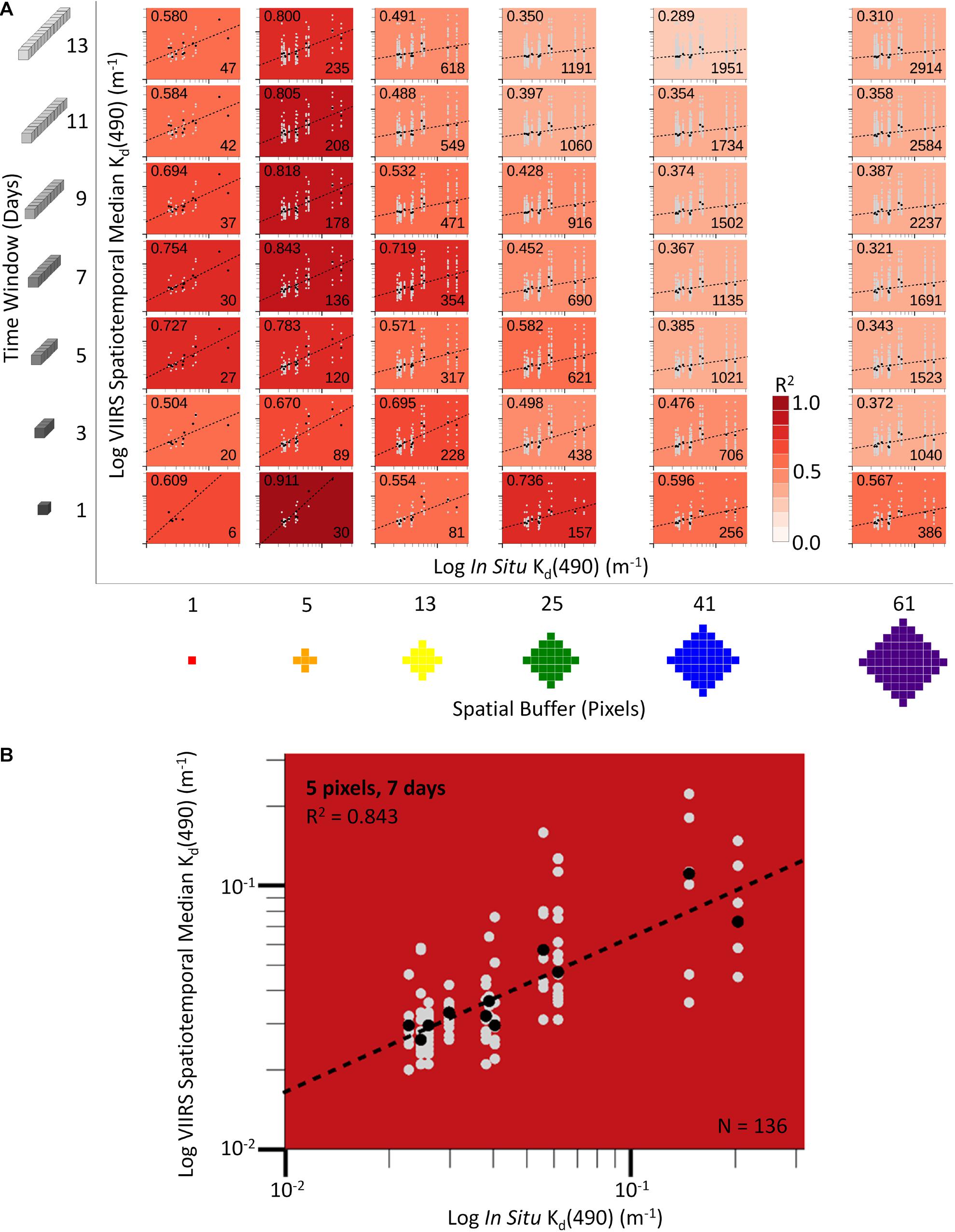
Figure 5. (A) Correlation matrix of in situ and VIIRS measures of log-transformed K_d(490) over a three-days in situ measurement period at 11 West Maui locations (Figure 2) for a range of spatial buffers and time windows applied to the satellite data. The outer horizontal axis indicates the spatial buffer and the outer vertical axis represents the time window, with icons on each representing the space (or time) domain. Together, the time window and spatial buffer make the spatiotemporal cube of satellite data from which values are compiled (gray circles) and the median of those is calculated (black circles). Shading of each plot represents the R² value of individual regression lines between the median satellite observation and the in situ observations. For each scatterplot, the horizontal axis values are the in situ observations from the sites in Figure 2, all of which were taken during November 26–28, 2018, and the vertical axis values are all satellite observations associated with that in situ measurement within the time window and space buffer indicated. The number in the upper left corner is the R² value for that plot; the number in the bottom right corner is the total number of satellite observations (gray circles) displayed in the plot. (B) Enlarged scatterplot for recommended spatiotemporal aggregation (5-pixels, 7-days). Axis tick values in (B) are the same as all scatterplots in (A) and major tick marks are bold for all scatterplots.

FIGURE 6

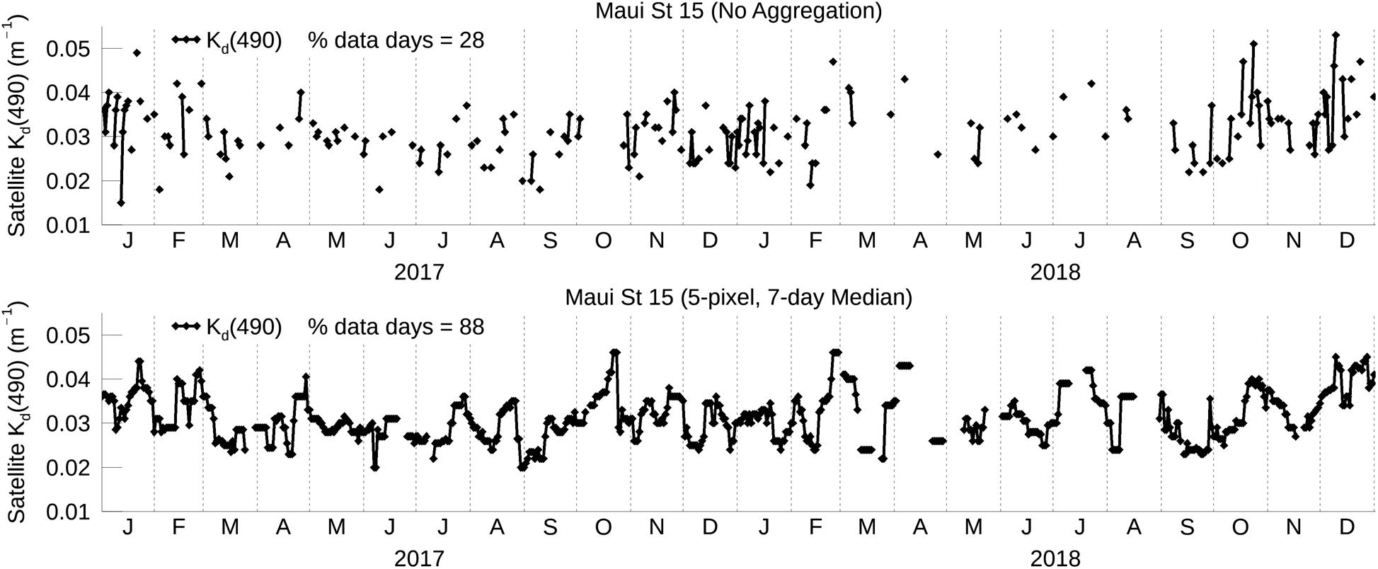
Figure 6. Time Series of K_d(490) from 2017 to 2018 at Maui Station 15 before aggregation (top) and after taking the median from a rolling 5-pixels, 7-days spatiotemporal window centered on the date (bottom) demonstrating improved data coverage. The RMS difference between the non-aggregated and aggregated time series is 0.005 m⁻¹.

Comparing Aggregated VIIRS K_d(490) With Onshore in situ Turbidity (NTU)—Maui

Having determined from the nearshore analysis that the 5-pixels, 7-days spatiotemporal aggregation was optimal, this aggregation scale was applied to VIIRS K_d(490) values for comparison with the onshore turbidity measurements. While some of the 51 onshore sites fell within the same 750 m pixel, the sampling dates were unique to each site. From the resulting matched sets of satellite and in situ data, the chronic or long-term turbidity at each site was determined using the median value through time to investigate variation with latitude (Figure 4). The left panel of Figure 4 illustrates the chronic spatial pattern of measured turbidity and K_d(490). Along the southern sector of the Maui coast, both measures increased from south to north until reaching Kalepolepo Park (∼20°46.6′ N). Variability in turbidity (as indicated by the interquartile whiskers), also increased along this section of the coast. In the middle latitudes, the coastline runs from east to west, from Kalepolepo Park around the bight to Mā'alaea Harbor, which means the values are difficult to distinguish by latitude alone (Figure 4). Considering the sites by index (Supplementary Figure 2 and Supplementary Table 2) this region experienced low turbidity values, while K_d(490) values remained high (index 19–23). Additionally, Mā'alaea Condos, Keālia Pond, and Haycraft Park (index 27–29), also within the bight, had low turbidity and high K_d(490) values. Along the northern sector of the Maui coast, turbidity (together with variability) increased heading north to Kā'opala Bay, although to a lesser extent than the southern sector. The northernmost site, Honolua Bay, had the highest variability in turbidity. Despite the differences in the measured quantities (in situ turbidity of particulates, and remotely sensed attenuation coefficient, which measures the effect of both particulates and dissolved matter), there is a consistency in the spatial pattern, indicating either that the components co-vary or that the satellite measurement is predominated by particulates. The R² between the long-term median K_d(490) and turbidity values was 0.056. While spatial patterns in the chronic conditions appeared consistent for the two datasets, there was little to no relationship between turbidity values and VIIRS K_d(490) when examined for each time and location. This was likely due to the inability of the satellite to measure changes in turbidity within tens of meters of the coast where turbidity samples were taken (typically <1 m deep water).

Comparing Aggregated VIIRS K_d(490) With in situ K_d(490)—Puerto Rico

We matched 22 in situ K_d(490) measurements spanning four years from a single nearshore site in Puerto Rico with spatiotemporal aggregations of satellite data (Figure 3, which shows satellite K_d(490) coverage for one matchup date). In situ and satellite K_d(490) values ranged between 0.03 and 0.33 m^–1. Median values from each spatiotemporal cube of VIIRS K_d(490) were compared with in situ K_d(490) measurements, and linear regressions of log-transformed data resulted in R² values ranging from 0.003 to 0.547 (Figure 7). Every spatiotemporal cube smaller than 13-pixels and/or shorter than nine days resulted in an R² less than 0.35. The highest R² of 0.547 (to three decimal places) resulted from the 13-pixels, 13-days and the 25-pixels, 13-days combinations (the latter was higher in the 5th decimal place). There was little difference in R² between the regressions that fell within the 13–41 pixels and 9–13 days range of the matrix (ranging 0.45–0.547). The 13-pixels, 13-days matchup yielded the highest R² with the more parsimonious spatial scale (Figure 7B). In contrast to the West Maui dataset, the in situ values here represent measurement dates at the same location rather than measurements across different sites. The matrix in Figure 7 shows little pattern between R² and increasing time and space scales, but it could be argued that increasing the time scale had a greater (positive) effect on R² than increasing the spatial scale. Evaluation of model fit using the RRMSE statistic (RRMSE < 15%) supported the selection of the 13-pixels, 13-days aggregation (using R²) to balance the desired improvement to data coverage (number of dates matched) while maintaining representation of the in-water measurements (Supplementary Figure 4). No spatiotemporal aggregation resulted in all in situ sampling dates having matched satellite data (the largest cube, 61-pixels and 13-days, matched with 19 out of 22 dates; the selected 13-pixels, 13-days cube matched with 17). Applying the 13-pixels, 13-days aggregation to Site LP6 resulted in an increase from 11 to 82% data coverage with an RMS difference of 0.025 m⁻¹ between the two time series (Figure 8).

FIGURE 7

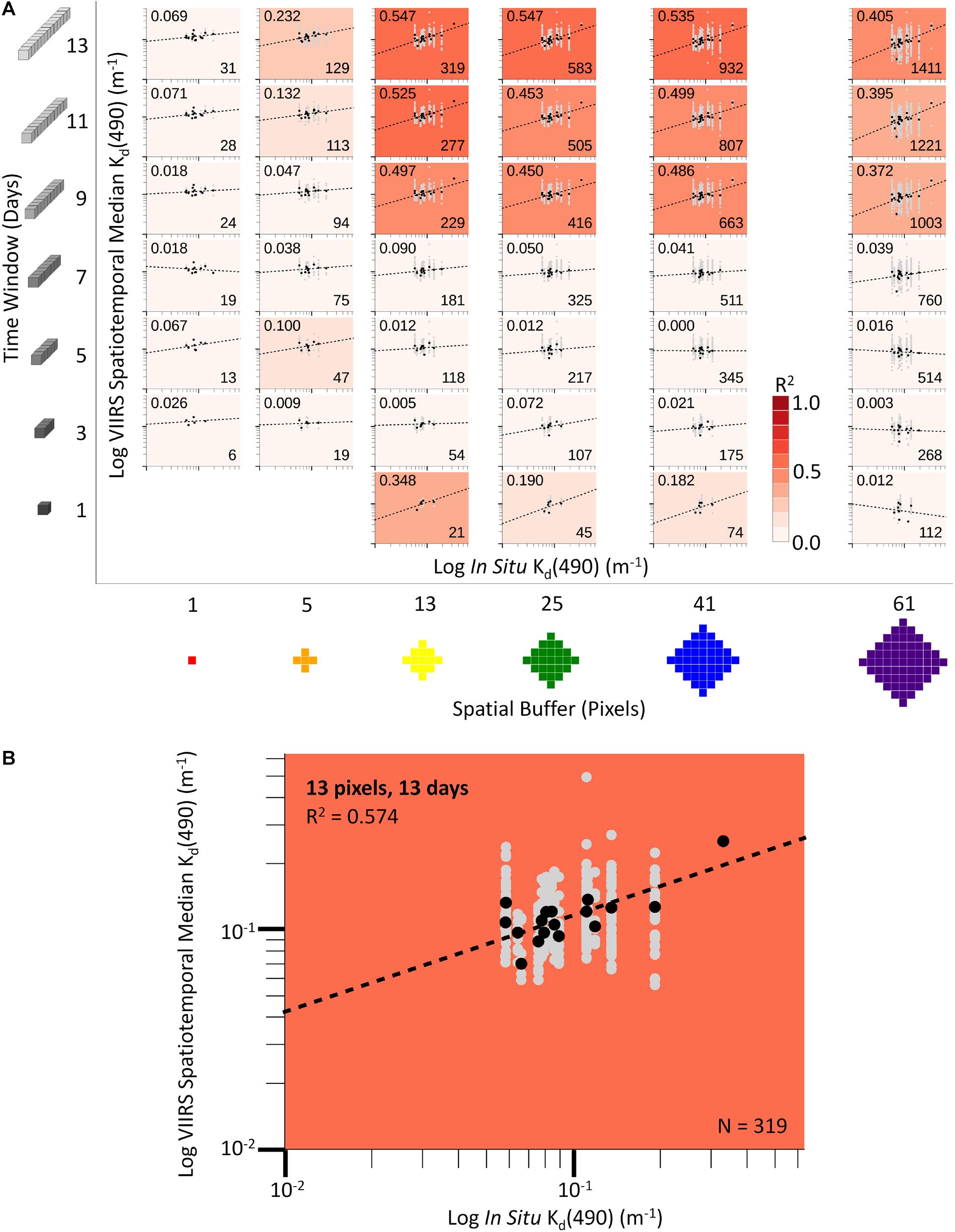
Figure 7. (A) Correlation matrix of in situ and VIIRS measures of log-transformed K_d(490) over a 4-years in situ measurement period at one southwest Puerto Rico location (Figure 5) for a range of spatial buffers and time windows applied to the satellite data. The outer horizontal axis indicates the spatial buffer and the outer vertical axis represents the time window, with icons on each representing the space (or time) domain. Together, the time window and spatial buffer make the spatiotemporal cube of satellite data from which satellite values are compiled (gray circles) and the median of those is calculated. Shading of each plot represents the R² value of individual regression lines between the median satellite observation and the in situ observations. Scatterplots with two or fewer matchups are excluded. For each scatterplot, the horizontal axis values are the in situ observations from the site in Figure 3, which were taken between 2016 and 2019, and the vertical axis values are all satellite observations associated with that in situ measurement within the time window and space buffer indicated. The number in the upper left corner is the R² value for that plot; the number in the bottom right corner is the total number of satellite observations (gray circles) displayed in the plot. (B) Enlarged scatterplot for recommended spatiotemporal aggregation (13-pixels, 13-days). Axis tick values in (B) are the same as all scatterplots in (A) and major tick marks are bold for all scatterplots.

FIGURE 8

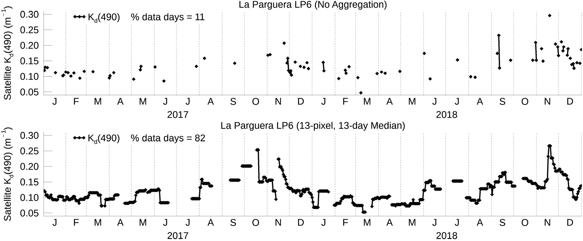
Figure 8. Time Series of K_d(490) from 2017 to 2018 at La Parguera, Puerto Rico Station LP6 before aggregation (top) and after taking the median from a rolling 13-pixels, 13-days spatiotemporal window centered on the date (bottom). The RMS difference between the non-aggregated and aggregated time series is 0.025 m⁻¹.

Discussion

Understanding the long- and short-term variations in water quality are essential to enhance related management of marine ecosystems. We found that aggregated VIIRS K_d(490) data adequately captures this variability in coastal waters, allowing characterization of water quality over broad regions. Researchers and managers can leverage the long time domain of satellite measures of water quality that are now available to assess both historical trends and variability, and to evaluate temporal dynamics. Our method of optimizing satellite data aggregation in nearshore areas, which are typically of low data density, successfully represented in situ measurements, supporting the use of this type of data for coral reefs and other coastal marine environments.

The nearshore Maui dataset—collected in a three-days snapshot at 11 sites—captured K_d(490) data over the West Maui region. The relationship between in situ K_d(490) and median VIIRS K_d(490) from a 5-pixels, 7-days spatiotemporal cube was robust at differentiating observations even across these small space and time domains. Many of the nearshore in situ K_d(490) measurement locations in Maui were within the satellite pixel directly adjacent to the VIIRS dataset land mask. This affected the overall number of pixels that had valid data and effectively reduced the total possible pixels in the spatiotemporal cubes by approximately half. Rather than attempting to shift the buffer to include additional water pixels and capture the maximum possible pixels for each buffer size, we chose instead to use a consistent method for all in situ sites. Time series using the 5-pixels, 7-days spatiotemporal cube at site 15 in Maui highlight the improvement in data coverage, while maintaining features of the non-aggregated data (Figure 7).

The robustness of the methodology also was apparent in the Puerto Rico analysis, which considered a single location over a longer time period (four years). However, the optimal spatiotemporal cube dimension (13-pixels, 13-days) was notably different. Aggregating satellite data over longer time and broader spatial scales yielded better correlation with in situ data, with a preference for longer time scales. This is consistent with previous uses of VIIRS monthly K_d(490) and chlorophyll-a data to monitor prolonged degradation of water quality after Hurricanes Maria and Irma in Puerto Rico (Hernández et al., 2020). Of the 22 in situ measurements, less than half had matching satellite data at combinations less than a 25-pixels spatial buffer or a 7-days time window. This can be explained by the typical occurrence of cloud cover at the time of the satellite overpass (Mikelsons and Wang, 2019; Hernández et al., 2020). However, the strength of the relationship between satellite and in situ data for larger spatiotemporal cubes suggests the persistence of water quality features in this region typically aligns with the scale selected for the aggregation. Importantly, and similar to the spatial analysis in Maui, VIIRS data seem capable of effectively capturing temporal dynamics in turbidity in Puerto Rico. Time series using the 13-pixels, 13-days spatiotemporal cube at site LP6 in La Parguera, Puerto Rico highlight the improvement in data coverage, while maintaining features of the non-aggregated data (Figure 8).

VIIRS K_d(490) also appear to be useful for monitoring and characterizing chronic states along the Maui coast where sediment input is known to be high and extends far offshore. The onshore turbidity dataset for Maui provided a spatially well-distributed dataset spanning three years, reflecting the commitment of both local organizations and state agencies to ongoing water quality monitoring. While turbidity and K_d(490) are measures of different in-water constituents (turbidity measures particles and K_d(490) measures both particles and dissolved matter), K_d(490) has been previously used to estimate turbidity levels in the Great Lakes (Son and Wang, 2019), and may act as a proxy for turbidity in particle-dominated waters. The similar spatial patterns of long-term conditions between in situ and satellite measures across south and west Maui suggest that nearshore patterns reflect those in shallow onshore waters. This provides confidence in the application of satellite data to inform likely onshore spatial patterns. Notably, the increase in both chronic VIIRS K_d(490) and turbidity from south to north follows known sedimentation patterns in Maui related to historic agricultural land use practices, as shown in the map in Figure 4. Historical pineapple plantations were common in the northern West Maui watersheds and best management practices were typically poor, such as terrace creation leading to movement of soil into the adjacent stream gulch (Stock et al., 2015). Along the northern coast, the turbidity gradient is also related to an increase in rainfall moving north to Honolua Bay. In the southern sector, large sugar plantations were in cultivation up until 2016, and were developed using an extensive network of ditches that also deliver sediment and nutrients to the coast. The effects were concentrated in the Mā'alaea area, which may partially explain the south-to-north increase in turbidity along the southern sector. It is of note that while spatial patterns in long-term characteristics were similar, individually paired turbidity values and VIIRS K_d(490) showed little to no relationship (maximum R² = 0.013 across all spatiotemporal cubes tested). This may be attributed to aforementioned differences in the in-water constituents satellite K_d(490) and in situ turbidity are measuring and the resolution and onshore coverage limitations of the satellite. Sediment resuspension with wind or wave action may also affect onshore samples differently from nearshore patterns we see in the satellite data. Although broad spatial patterns are captured by satellite data, the temporal variability of particular sites is not well captured, emphasizing the independent value of in situ sampling.

Importantly, these results together indicate the complementary value of using both remotely sensed and in situ data on water quality. Satellite products can provide continuity of information between field excursions, while in-water measurements are invaluable during extended periods of cloud cover that usually correlate with storms and occur close to shore, where bottom reflectance and land masking prevent consistently available satellite data. In the shallow coastal zone, satellite products may best inform long-term conditions (e.g., baseline data) for water quality that couple with in situ data used to monitor short-term events. For some sites, it may be possible to develop satellite tools that alert managers and other stakeholders to unusual conditions nearshore, which trigger response monitoring onshore. Similarly, in situ measurements can be useful to inform the development of satellite algorithms in complex waters.

It is common practice to average satellite data over longer time scales of weeks and months to understand seasonal patterns and fill data gaps. It is less common to increase the spatial buffer used, especially near the coast, due to the potential of introducing more noise into the signal. However, for monitoring changes over an area, such as coastal coral reefs, this method of determining the optimal spatiotemporal scale may capture nearby events that can have ecological impacts, such as a sediment plume moving along the coast. While they can be informed by the analyses presented here, optimizing the dimensions of the spatiotemporal aggregation should ideally be undertaken for each geographic region of study using appropriate in situ measurements. This is especially important since satellite data coverage can vary greatly from location to location. Spatial buffer size may ultimately affect the correlation between satellite and in situ data when trying to track acute events; however, it can be useful for characterizing the chronic state of a location when looking for anomalies. Our relationships between satellite data and in situ data in Maui and Puerto Rico suggest that aggregating over longer time scales produces better correlations with in situ data than increasing spatial buffer size; however, further analysis would be required to categorically state this.

Enhancing the availability of temporally dense, long-term satellite data to managers opens up new possibilities for application and calibration/validation. The application of methods to maximize satellite data availability should include fine-tuning with in situ measurements at each new location. Ecological models that require regular data input to generate predicted changes in environmental conditions, such as seagrass habitat loss or coral disease occurrence, could utilize this method. We suggest testing this method with other remotely sensed metrics such as chlorophyll-a or colored dissolved organic matter (CDOM) where in situ data are readily available. Longer time series of in situ water quality data in nearshore and onshore environments would benefit the validation and applicability of this method.

Conclusion

Remotely sensed ocean color data from satellites provide useful information for characterizing and tracking changes in water quality over broad regions. Many challenges exist when creating management tools using these data, the most prevalent of which are data gaps due to clouds and capturing events that occur at small spatial and temporal scales close to the coast (e.g., tens of meters, less than one day in duration). In this study, we addressed the issue of overcoming data gaps by testing space and time aggregation methods on VIIRS data in Maui Hawai‘i and southwestern Puerto Rico to determine when the correlation with corresponding in situ measurements is optimal. We found that this method worked well in nearshore waters of Maui for optimizing the correlation with in situ data and increasing the overall number of satellite matchups. In onshore waters in Maui, VIIRS data aggregated with this method follow similar climatological patterns as in situ turbidity measurements over a 3-years period. In Puerto Rico, the overall correlations between VIIRS data and in situ data were lower, but R² and matchups were maximized at longer time and space scales. The complementary nature of satellite and in situ water quality measurements enhance our understanding of coastal ecosystems and should continue to be used together in management plans and other applications.

Data Availability Statement

The raw data supporting the conclusions of this article will be made available by the authors, without undue reservation.

Author Contributions

EFG, SFH, WJH, JMC, MJD, and ALG contributed to conception and design of the study. WJH, RAA, KF, and TC provided in situ data. EFG, SFH, MJD, JMC, WJH, CME, and ALG conceptualized and/or performed the statistical analysis. EFG wrote the first draft of the manuscript with WJH, KF, and SFH contributing sections of the manuscript. EFG, SFH, WJH, JMC, KF, TC, ALG, GL, JLD, RAA, MJD, and CME contributed to manuscript revision, read, and approved the submitted version.

Funding

Funding for this study is from the NASA Ecological Forecasting program grant NNX17AI21G. Coral Reef Watch staff and this study were partially supported by NOAA grant NA19NES4320002 (Cooperative Institute for Satellite Earth System Studies) at the University of Maryland/ESSIC. The in situ optical measurements (WJH and RAA) were supported in part by the National Oceanic and Atmospheric Administration-Cooperative Science Center for Earth System Sciences and Remote Sensing Technologies (NOAA-CESSRST) under Cooperative Agreement Grant # NA16SEC4810008, as well as via funding from the NOAA Product Development, Readiness and Application (PDRA, Ocean Remote Sensing). The in situ turbidity data were collected with support from the County of Maui, National Fish and Wildlife Foundation, the Makana Aloha Foundation, Fred Baldwin Memorial Foundation, Honua Kai West Maui Community Fund, Inc., Napili Bay and Beach Foundation, Lush Cosmetics Charity Pot, and the State of Hawai‘i, Department of Health.

Conflict of Interest

EFG, WJH, GL, JLD, and CME were employed by, and SFH subcontracted to, the company Global Science and Technology, Inc.

The remaining authors declare that the research was conducted in the absence of any commercial or financial relationships that could be construed as a potential conflict of interest.

Acknowledgments

We would like to acknowledge the University of Puerto Rico, Mayagüez (with special thanks to Suhey Ortiz-Rosa) and the support of the University of Hawai‘i at Manoa in the acquisition of in situ optical measurements in Puerto Rico and/or West Maui; Hui o Ka Wai Ola volunteers, funders and supporting organizations (The Nature Conservancy, Maui Nui Marine Resource Council and the West Maui Ridge to Reef Initiative) for providing in situ turbidity measurements for West Maui; and the NOAA Center for Satellite Applications and Research CoastWatch and Ocean Color Teams for providing VIIRS satellite data. Our thanks to Jordan Dennis for undertaking initial exploratory analysis of the onshore data. The scientific results and conclusions, as well as any views or opinions expressed herein, are those of the author(s) and do not necessarily reflect the views of NOAA or the Department of Commerce.

Supplementary Material

The Supplementary Material for this article can be found online at: https://www.frontiersin.org/articles/10.3389/fmars.2021.643302/full#supplementary-material

Supplementary Figure 1 | Range of normalized E_d(490) from three separate casts using a Sea-Bird Scientific HyperPro II optical profiler at (A) Station 15 in West Maui on November 28, 2018 and (B) Station LP6 in La Parguera, Puerto Rico on December 6, 2017.

Supplementary Figure 2 | Temporal median of the time series of (red, right axis) in situ turbidity (NTU) and (black, left axis) spatiotemporal (median of 5-pixels, 7-days cube) satellite K_d(490) (m^–1) for each site by index number in West Maui, HI. Site latitude increases from left to right with index number (see Figure 4, left panel).

Supplementary Figure 3 | (A) Correlation matrix of in situ and VIIRS measures of log-transformed K_d(490) over a 3-days in situ measurement period at 11 West Maui locations (Figure 2) for a range of spatial buffers and time windows applied to the satellite data. The outer horizontal axis indicates the spatial buffer and the outer vertical axis represents the time window, with icons on each representing the space (or time) domain. Together, the time window and spatial buffer make the spatiotemporal cube of satellite data from which values are compiled (gray circles) and the median of those is calculated (black circles). Shading of each plot represents the RRMSE value of individual regression lines between the median satellite observation and the in situ observations. For each scatterplot, the horizontal axis values are the in situ observations from the sites in Figure 2, all of which were taken during November 26–28, 2018, and the vertical axis values are all satellite observations associated with that in situ measurement within the time window and space buffer indicated. The number in the upper left corner is the RRMSE value for that plot; the number in the bottom right corner is the total number of satellite observations (gray circles) displayed in the plot. (B) Enlarged scatterplot for recommended spatiotemporal aggregation (5-pixels, 7-days). Axis tick values in (B) are the same as all scatterplots in (A) and major tick marks are bold for all scatterplots.

Supplementary Figure 4 | (A) Correlation matrix of in situ and VIIRS measures of log-transformed K_d(490) over a 4-years in situ measurement period at one southwest Puerto Rico location (Figure 5) for a range of spatial buffers and time windows applied to the satellite data. The outer horizontal axis indicates the spatial buffer and the outer vertical axis represents the time window, with icons on each representing the space (or time) domain. Together, the time window and spatial buffer make the spatiotemporal cube of satellite data from which satellite values are compiled (gray circles) and the median of those is calculated. Shading of each plot represents the RRMSE value of individual regression lines between the median satellite observation and the in situ observations. Scatterplots with two or fewer matchups are excluded. For each scatterplot, the horizontal axis values are the in situ observations from the site in Figure 3, which were taken between 2016 and 2019, and the vertical axis values are all satellite observations associated with that in situ measurement within the time window and space buffer indicated. The number in the upper left corner is the RRMSE value for that plot; the number in the bottom right corner is the total number of satellite observations (gray circles) displayed in the plot. (B) Enlarged scatterplot for recommended spatiotemporal aggregation (13-pixels, 13-days). Axis tick values in (B) are the same as all scatterplots in (A) and major tick marks are bold for all scatterplots.

Supplementary Table 1 | Site names, locations, and average depths of in situ measurement sites. The date the Maui samples were taken is November 28, 2018 and the date of the La Parguera sample is December 6, 2017. Apparent optical depth was calculated using the formula 1.3/K_d (Bailey and Werdell, 2006). Rows with a gray background are considered optically shallow since the apparent optical depth exceeds the site average depth.

Supplementary Table 2 | West Maui, HI sites where in situ turbidity samples were taken sorted by descending latitude as they appear in Figure 4. N Observations is the total number of in situ observations, Matched Pairs is the number of in situ observations with corresponding satellite observations (within the 5-pixels, 7-days data cube), and Distance to Satellite Pixel is the distance of the in situ observation to the center point of the 750 m satellite pixel containing the sampling site (decimal degrees).

Supplementary Table 3 | List of Level-2 flags used for quality control during the binning process and corresponding bit values that make up the bitmask for flagging data.

References

Bailey, S. W., and Werdell, P. J. (2006). A multi-sensor approach for the on-orbit validation of ocean color satellite data products. Remote Sens. Environ. 102, 12–23. doi: 10.1016/j.rse.2006.01.015

CrossRef Full Text | Google Scholar

Barnes, B. B., Garcia, R., Hu, C., and Lee, Z. (2018). Multi-band spectral matching inversion algorithm to derive water column properties in optically shallow waters: An optimization of parameterization. Remote Sens. Environ. 204, 424–438. doi: 10.1016/j.rse.2017.10.013

CrossRef Full Text | Google Scholar

Barnes, B. B., Hu, C., Schaeffer, B. A., Lee, Z., Palandro, D. A., and Lehrter, J. C. (2013). MODIS-derived spatiotemporal water clarity patterns in optically shallow Florida Keys waters: A new approach to remove bottom contamination. Remote Sens. Environ. 134, 377–391. doi: 10.1016/j.rse.2013.03.016

CrossRef Full Text | Google Scholar

Burke, L., Reytar, K., Spalding, M., and Perry, A. (2011). Reefs at Risk Revisited. Washington, DC: World Resources Institute.

Google Scholar

Carpenter, K. E., Abrar, M., Aeby, G., Aronson, R. B., Banks, S., Bruckner, A., et al. (2008). One-third of reef-building corals face elevated extinction risk from climate change and local impacts. Science 321, 560–563.

Google Scholar

Duan, W., He, B., Takara, K., Luo, P., Nover, D., Sahu, N., et al. (2013). Spatiotemporal evaluation of water quality incidents in japan between 1996 and 2007. Chemosphere 93, 946–953. doi: 10.1016/j.chemosphere.2013.05.060

PubMed Abstract | CrossRef Full Text | Google Scholar

Fabricius, K. E. (2005). Effects of Terrestrial Runoff on the Ecology of Corals and Coral Reefs: Review and Synthesis. Mar. Pollut. Bull. 50, 125–146. doi: 10.1016/j.marpolbul.2004.11.028

PubMed Abstract | CrossRef Full Text | Google Scholar

Feng, L., and Hu, C. (2015). Comparison of Valid Ocean Observations Between MODIS Terra and Aqua Over the Global Oceans. IEEE Transact. Geosci. Remote Sens. 54, 1–11. doi: 10.1109/TGRS.2015.2483500

CrossRef Full Text | Google Scholar

Gholizadeh, M. H., Melesse, A. M., and Reddi, L. A. (2016). Comprehensive Review on Water Quality Parameters Estimation Using Remote Sensing Techniques. Sensors 16:1298. doi: 10.3390/s16081298

PubMed Abstract | CrossRef Full Text | Google Scholar

Hernández, W. J., Ortiz-Rosa, S., Armstrong, R. A., Geiger, E. F., Eakin, C. M., and Warner, R. A. (2020). Quantifying the Effects of Hurricanes Irma and Maria on Coastal Water Quality in Puerto Rico using Moderate Resolution Satellite Sensors. Remote Sens. 12:964. doi: 10.3390/rs12060964

CrossRef Full Text | Google Scholar

Hu, C., Barnes, B. B., Feng, L., Wang, M., and Jiang, L. (2020). On the Interplay Between Ocean Color Data Quality and Data Quantity: Impacts of Quality Control Flags. IEEE Geosci. Remote Sens. Lett. 17, 745–749. doi: 10.1109/LGRS.2019.2936220

CrossRef Full Text | Google Scholar

Hu, C., Barnes, B. B., Murch, B., and Carlson, P. (2014). Satellite-based virtual buoy system (VBS) to monitor coastal water quality. Optic. Engine. 53:051402. doi: 10.1117/1.OE.53.5.051402

CrossRef Full Text | Google Scholar

Hughes, T. P., Anderson, K. D., Connolly, S. R., Heron, S. F., Kerry, J. T., Lough, J. M., et al. (2018). Spatial and temporal patterns of mass bleaching of corals in the Anthropocene. Science 359, 80–83. doi: 10.1126/science.aan8048

PubMed Abstract | CrossRef Full Text | Google Scholar

Kirk, J. T. O. (2011). Light and photosynthesis in aquatic ecosystems. Cambridge: Cambridge University Press.

Google Scholar

Lee, Z. P., Du, K., and Arnone, R. (2005). A model for the diffuse attenuation coefficient of downwelling irradiance. J. Geophys. Res. 110: 2275.

Google Scholar

Lee, Z., Pahlevan, N., Ahn, Y., Greb, S., and O’Donnell, D. (2013). Robust approach to directly measuring water-leaving radiance in the field. Appl. Opt. 52, 1693–1701. doi: 10.1364/ao.52.001693

PubMed Abstract | CrossRef Full Text | Google Scholar

Lesser, M. P., Slattery, M., and Leichter, J. J. (2009). Ecology of Mesophotic Coral Reefs. J. Exp. Mar. Biol. Ecol. 1, 1–8. doi: 10.1016/j.jembe.2009.05.009

CrossRef Full Text | Google Scholar

Liu, X., and Wang, M. (2018). Gap Filling of Missing Data for VIIRS Global Ocean Color Products Using the DINEOF Method. IEEE Transact. Geosci. Remote Sens. 56, 4464–4476. doi: 10.1109/TGRS.2018.2820423

CrossRef Full Text | Google Scholar

Liu, X., and Wang, M. (2019). Filling the Gaps of Missing Data in the Merged VIIRS SNPP/NOAA-20 Ocean Color Product Using the DINEOF Method. Remote Sens. 11:178. doi: 10.3390/rs11020178

CrossRef Full Text | Google Scholar

McKinna, L., and Werdell, J. (2018). Approach for identifying optically shallow pixels when processing ocean-color imagery. Opt. Express 26, A915–A928.

Google Scholar

Mikelsons, K., and Wang, M. (2019). Optimal satellite orbit configuration for global ocean color product coverage. Opt. Express 27, A445–A457.

Google Scholar

Morel, A., Huot, Y., Gentili, B., Werdell, P. J., Hooker, S. B., and Franz, B. A. (2007). Examining the consistency of products derived from various ocean color sensors in open ocean (Case 1) waters in the perspective of a multi-sensor approach. Remote Sens. Environ. 111, 69–88. doi: 10.1016/j.rse.2007.03.012

CrossRef Full Text | Google Scholar

Mueller, J., Morel, A., Frouin, R., Davis, C., Arnone, R., Carder, K., et al. (2003). Ocean Optics Protocols for Satellite Ocean Color Sensor Validation, Revision 4, Volume III: Radiometric Measurements and Data Analysis Protocols. Washington, D.C: NASA, 78.

Google Scholar

Nearing, M. A., Jetten, V., Baffaut, C., Cerdan, O., Couturier, A., et al. (2005). Modeling response of soil erosion and runoff to changes in precipitation and cover. CATENA 61, 131–154. doi: 10.1016/j.catena.2005.03.007

CrossRef Full Text | Google Scholar

NOAA (2021). NOAA Coastwatch. Washington, D.C: NOAA.

Google Scholar

Ondrusek, M., Stengel, E., Kinkade, C., Vogel, R., Keegstra, P., Hunter, C., et al. (2012). The development of a new optical total suspended matter algorithm for the Chesapeake Bay. Remote Sens. Environ. 119, 243–254. doi: 10.1016/j.rse.2011.12.018

CrossRef Full Text | Google Scholar

Otaño-Cruz, A., Montañez-Acuña, A. A., Torres-López, V., Hernández-Figueroa, E. M., and Hernández-Delgado, E. A. (2017). Effects of Changing Weather, Oceanographic Conditions, and Land Uses on Spatio-Temporal Variation of Sedimentation Dynamics along Near-Shore Coral Reefs. Front. Mar. Sci. 4:249. doi: 10.3389/fmars.2017.00249

CrossRef Full Text | Google Scholar

Pandolfi, J. M., Bradbury, R. H., Sala, E., Hughes, T. P., Bjorndal, K. A., Cooke, R. G., et al. (2003). Global trajectories of the long-term decline of coral reef ecosystems. Science 301.5635, 955–958. doi: 10.1126/science.1085706

PubMed Abstract | CrossRef Full Text | Google Scholar

Pollock, F. J., Lamb, J. B., Field, S. N., Heron, S. F., Schaffelke, B., Shedrawi, G., et al. (2014). Sediment and Turbidity Associated with Offshore Dredging Increase Coral Disease Prevalence on Nearby Reefs. PLoS One 9:e102498. doi: 10.1371/journal.pone.0102498

PubMed Abstract | CrossRef Full Text | Google Scholar

Reichstetter, M., Fearns, P. R. C. S., Weeks, S. J., McKinna, L. I. W., Roelfsema, C., and Furnas, M. (2015). Bottom Reflectance in Ocean Color Satellite Remote Sensing for Coral Reef Environments. Remote Sens. 7, 16756–16777. doi: 10.3390/rs71215852

CrossRef Full Text | Google Scholar

Rodolfo-Metalpa, R., Hoogenboom, M. O., Rottier, C., Ramos-Esplá, A., Baker, A. C., Fine, M., et al. (2014). Thermally tolerant corals have limited capacity to acclimatize to future warming. Glob. Change Biol. 20, 3036–3049. doi: 10.1111/gcb.12571

PubMed Abstract | CrossRef Full Text | Google Scholar

Rogers, C. S. (1990). Responses of coral reefs and reef organisms to sedimentation. Mar. Ecol. Prog. Ser. 62, 185–202. doi: 10.3354/meps062185

CrossRef Full Text | Google Scholar

Sathyendranath, S., Brewin, R. J., Brockmann, C., Brotas, V., Calton, B., Chuprin, A., et al. (2019). An Ocean-Colour Time Series for Use in Climate Studies: The Experience of the Ocean-Colour Climate Change Initiative (OC-CCI). Sensors 19:4285. doi: 10.3390/s19194285

PubMed Abstract | CrossRef Full Text | Google Scholar

Sheridan, C., Baele, J. M., Kushmaro, A., Fréjaville, Y., and Eeckhaut, I. (2014). Terrestrial runoff influences white syndrome prevalence in SW Madagascar. Mar. Environ. Res. 101, 44–51. doi: 10.1016/j.marenvres.2014.08.003

PubMed Abstract | CrossRef Full Text | Google Scholar

Son, S., and Wang, M. (2019). VIIRS-Derived Water Turbidity in the Great Lakes. Remote Sens. 11:1448. doi: 10.3390/rs11121448

CrossRef Full Text | Google Scholar

Stock, J. D., Falinski, K. A., and Callender, T. (2015). Reconnaissance sediment budget for selected watersheds of West Maui, Hawai‘i, USA. Hawai‘i: US Geological Survey, 44.

Google Scholar

Thompson, A., Schroeder, T., Brando, V. E., and Schaffelke, B. (2014). Coral community responses to declining water quality: Whitsunday Islands, Great Barrier Reef, Australia. Coral Reefs 33, 923–938. doi: 10.1007/s00338-014-1201-y

CrossRef Full Text | Google Scholar

UNEP (2017). Frontiers 2017: Emerging issues of environmental concern. Nairobi: United Nations Environment Programme, 36–37.

Google Scholar

Wang, M., Liu, X., Jiang, L., and Son, S. (2017). The VIIRS Ocean Color Products, in Algorithm Theoretical Basis Document Version 1.0. 68.

Google Scholar

Wang, M., Son, S., and Harding, L. W. Jr. (2009). Retrieval of diffuse attenuation coefficient in the Chesapeake Bay and turbid ocean regions for satellite ocean color applications. J. Geophys. Res. 114:5286.

Google Scholar

Weber, M., De Beer, D., Lott, C., Polerecky, L., Kohls, K., Abed, R. M., et al. (2012). Mechanisms of Damage to Corals Exposed to Sedimentation. Proc. Natl. Acad. Sci. 109, E1558–E1567. doi: 10.1073/pnas.1100715109

PubMed Abstract | CrossRef Full Text | Google Scholar

Wei, J., Lee, Z., and Shang, S. (2016). A system to measure the data quality of spectral remote-sensing reflectance of aquatic environments. J. Geophys. Res. Oceans 121:2016JC012126.

Google Scholar