Complementary Approaches to Assess Phytoplankton Groups and Size Classes on a Long Transect in the Atlantic Ocean

Introduction

Given present climate change scenarios, improved understanding of biogeochemical cycles, notably carbon, is crucial. The CO₂ cycle is affected greatly by primary production by plants on land and algae in the oceans. Chlorophyll a (Chla) has traditionally been used as a proxy for phytoplankton biomass and can be assessed by Earth Observation (EO) on synoptic spatial scales and over an increasing timespan (currently, 1997–2022).

Phytoplankton is a complex and diverse community constituted by several taxonomic classes, with cell sizes spanning from 0.6 to 200 μm, with different ecological roles and nutrient requirements. Phytoplankton size structure is acknowledged as a fundamental property controlling the ecological and biogeochemical functioning of pelagic ecosystems (Chisholm, 1992; Cermeño and Figueiras, 2008; Dutkiewicz et al., 2020). However, the identification and enumeration of taxa by microscopy is a time-consuming procedure, highly dependent on expertise, and impossible to undertake at the temporal and spatial resolution needed to assess the state of the oceans. Hence, there has been a strong focus on estimating phytoplankton community structure by measuring diagnostic pigments (Vidussi et al., 2001), whilst establishing the link with phytoplankton size classes (PSCs) (Uitz et al., 2006). Typically, three size classes have been described for phytoplankton: picoplankton (diameter <2 μm), nanoplankton (diameter from 2 to 20 μm) and microplankton (diameter >20 μm) (Sieburth et al., 1978), and their occurrence is strongly linked with oceanographic conditions.

Models relating PSC to the Chla concentration estimated by EO are well established (e.g., Hirata et al., 2008; Brewin et al., 2010; amongst others), and used in operational EO services such as the United Kingdom NERC EO Data Analysis and AI Service (NEODAAS¹) and the Copernicus Marine Environment Monitoring Service (CMEMS²). These models have been extensively validated with in situ data of photosynthetic pigments concentration from High Performance Liquid Chromatography (HPLC) in the water column (Brewin et al., 2012, 2017a; Brotas et al., 2013; Brito et al., 2015; Lamont et al., 2018; Liu et al., 2021; amongst others).

However, as Sathyendranath et al. (2020) pointed out, achieving a good estimation of phytoplankton global biomass and size structure in terms of carbon is paramount to our understanding of oceanic geological cycles. These authors stress that monitoring both Chla and carbon concentration in the ocean is mandatory to improve our knowledge of phytoplankton dynamics, stressing that it is not a matter of choice between Chla or carbon. Assessing carbon phytoplankton dynamics by EO is challenging, and in a review paper by Brewin et al. (2021), there is an increasing interest in satellite phytoplankton carbon products. This work notes that only a few approaches for detecting phytoplankton carbon products from space are available (Kostadinov et al., 2016; Jackson et al., 2017; Roy et al., 2017). In addition to PSCs, interest has also focused on retrieving phytoplankton functional group (PFT) abundance (see Nair et al., 2008; Hirata et al., 2011; Losa et al., 2017; amongst others) and is presently considered a priority in ocean colour remote sensing (see IOCCG, 2014; Bracher et al., 2017 for a review). The above goals are strongly connected, requiring a better understanding of the correspondence of PSC and PFT, on one side, and the possibility of assessment of phytoplankton size structure in terms of Carbon by EO, on the other side.

To address these questions, we used data collected along a transect in the Atlantic Ocean, covering a wide geographic range with distinct oceanographic environmental conditions. The Atlantic Meridional Transect (AMT³) is a long-term multidisciplinary research programme studying the Atlantic biogeochemistry and oceanography from ∼50° N to 50° S. The AMT programme constitutes one of the few long-term studies over the Atlantic Ocean, collecting data on wide variety of physical and biogeochemistry properties over a very large geographical range (Aiken et al., 2016). It was initiated in 1995 with biannual cruises, and after 2000 with annual cruises, sailing from the United Kingdom to the Falkland Islands, South Africa, or Chile (Rees et al., 2015). These authors describe the evolution of the objectives during the several phases of the programme. Two key AMT aims have been quantifying causes of variability in planktonic ecosystems and delivering ground-truth data for satellite missions. The phytoplankton community taxonomic composition has been studied in the AMT programme using Flow Cytometry (FC) (Tarran et al., 2001, 2006), FC and FlowCAM for the microplankton community groups Fileman et al. (2017), or by filter examination by Scanning Electronic Microscopy focusing only on Coccolithophores (Poulton et al., 2017). However, there is a lack of studies quantifying the cell numbers of the whole phytoplankton community, in particular, species with cell diameter >10 μm. Published results with species identification and enumeration only target the period between 1996 and 2000 (Sal et al., 2013); these data have been used in several works, such as Marañón et al. (2014) and Dutkiewicz et al. (2020).

The present work assesses phytoplankton community size structure using both pigments and carbon concentration (converted from cell enumeration) and applies the Brewin et al. (2010) model to both datasets, making this work the first attempt to apply the model to carbon data: this provides the basis to infer size fractionated carbon from EO data.

The main objectives of this study were the following: (i) to analyse and compare PSCs with two methodological approaches: the pigment approach and cell enumeration converted into carbon; (ii) to apply the abundance size class model of Brewin et al. (2010) to a size class abundance based on carbon, (iii) to study the biomass and composition of phytoplankton communities along distinct environmental conditions of the Atlantic Ocean, discussing the links between phytoplankton taxonomic groups, size classes, and functional types. The ultimate goal aims to contribute to strengthening the capability of assessing phytoplankton community structure and phytoplankton carbon budgets by satellite EO.

Materials and Methods

Sampling

This work was conducted on board the Royal Research Ship James Clark Ross within the AMT programme. The cruise took place from September 15th to November 3rd, 2015,⁴ along a track spanning from 50.033° N and 4.375° W to 49.777° S and 54.509° W. Figure 1 plots the cruise track over images of SST (Sea Surface Temperature) and Chla obtained for the whole cruise period.

FIGURE 1

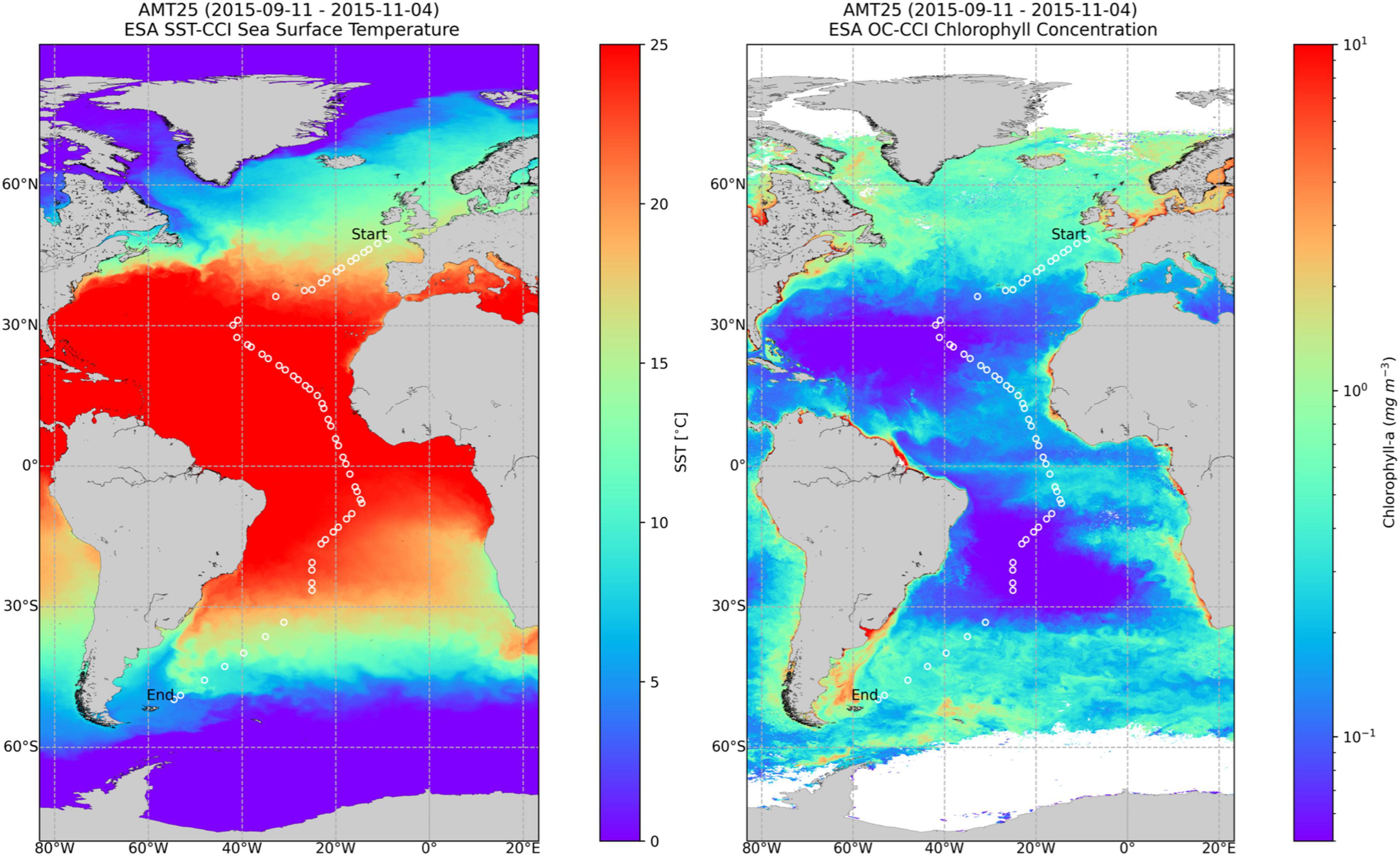
Figure 1. Composite images of Sea Surface Temperature (SST), left, and Chla, right, obtained from September 11, 2015 until November 4, 2015, showing the cruise track with the sampling stations. Chla image was obtained from the OC-CCI portal (www.oceancolour.org). Courtesy of NEODAAS.

Seawater samples were taken from 24 × 20 L OTE (Ocean Test Equipment) CTD bottles mounted on a stainless steel rosette frame and a Seabird CTD system. The samples were taken from the predawn and noon CTD casts.

For microscopic and flow cytometric enumeration of phytoplankton, and HPLC, only surface samples, taken from a water depth between 2 and 5 m were analysed. Nutrient samples were collected at every depth from each CTD cast according to GO-SHIP protocols.

Nutrients and Mixed Layer Depth

To determine nutrients content, water samples taken at each CTD cast were sub-sampled into clean (acid-washed) 60 mL HDPE (Nalgene) sample bottles, which were rinsed three times with sample seawater prior to filling and capping. The samples were analysed on the ship as soon as possible after sampling and were not stored or preserved.

Micro-molar nutrient analysis was carried out on board using a four channel SEAL analytical AAIII segmented flow nutrient auto-analyser. The colorimetric analysis methods used were: Nitrate (Brewer and Riley, 1965, modified), Nitrite (Grasshoff, 1976), and Phosphate and Silicate (Kirkwood, 1989). Sample handling and protocols were carried out where possible according to GO-SHIP protocols (Becker et al., 2020).

Mixed Layer Depth (MLD) was determined following the temperature criterion (Levitus, 1982), which defines the mixed layer as the depth at which temperature change from the surface value is 0.5°C.

Microscope Cell Identification and Counting

Samples were collected at 57 stations, at 2 or 5 m depth. For each sampling site, two samples of 200 mL were put in amber glass bottles; one fixed with neutral Lugol’s iodine solution (2% final concentration) and the other with formaldehyde (2% final concentration). In the laboratory, observations were carried out with a Zeiss Axiovert 200 inverted microscope. Cells >10 μm were counted in a 50 mL chamber, following the Utermöhl method (Utermöhl, 1958). Species from the following divisions/classes were identified and counted from Lugol’s-fixed samples: Bacillaryophyceae (Diatoms), Dinophyceae, separated into ADinos and heterotrophic dinoflagellates (HDinos), Prasinophyceae; furthermore the genus Phaeocystis and filamentous cyanobacteria belonging to three genera were also quantified. These groups were defined according to work carried out on AMTs 1 to 10, from which a database of taxa identified by microscopy is presented (Sal et al., 2013). The distinction between autotrophic and heterotrophic dinoflagellate species followed the same database.

For the formaldehyde bottle, only coccolithophore species >10 μm were identified and enumerated (due to coccolith degradation in Lugol’s-fixed samples).

Species identifications were checked against species records of AMTs 1, 3, 5, and 7, which occurred in Boreal Autumn, in common with the 25th Atlantic Meridional Transect (AMT25) cruise.

Flow Cytometer Cell Analysis

Samples were collected in clean 250 mL polycarbonate bottles from the CTD system, stored in a refrigerator and analysed within 3 h of collection. Fresh samples were analysed using a Becton Dickinson FACSort flow cytometer. Within the analysis window it was possible to resolve six different groups: Prochlorococcus spp., Synechococcus spp., pico-eukaryotes (PEUK), coccolithophores within 5–8 μm (COCCOS), cryptophytes (CRYPTO), and other nanophytoplankton (NEUK), following the methodology described in Tarran et al. (2006).

Flow cytometer targets the smaller component of phytoplankton cells, from equivalent spherical diameter (ESD) of <1 μm up to ca 10 μm, whereas microscopy may identify cells with ESD ≥10 μm.

Cell Carbon Estimates

In order to compare all components of the phytoplankton community, cell abundance of each taxa was converted into carbon content (mg carbon m^–3).

For phytoplankton cells counted by microscopy, the cell carbon content was obtained mainly from the AMT database published by Sal et al. (2013). For species absent in the AMT database, biovolume was converted to cell carbon using the conversion factors presented by Menden-Deuer and Lessard (2000). Species biovolume was calculated either from measurements using photographic images taken during this study, using the geometrical forms indicated by Hillebrand et al. (1999), Sun and Liu (2003), and Olenina et al. (2006), or if not possible, from the species biovolume indicated by Olenina et al. (2006). It should be noted that the estimation of carbon content through biovolume implies a certain bias in the data, as in larger cells the carbon content is probably overestimated in comparison to smaller cells, where the cellular content is more tightly packed.

For filamentous and colonial species, the total number of cells was estimated by measuring the cell dimension, and the length of the filament or colony. Then, biovolume and carbon conversion factors were applied.

For cells measured by flow cytometry, cell numbers of Prochlorococcus and Synechococcus were converted to cell carbon by applying conversion factors of 32 and 110 fg carbon cell^–1, respectively, following Tarran et al. (2001). Cell carbon content factors for PEUK, NEUK, CRYPTO, and COCCOS, were 0.44, 3.53, 23.66, and 33.37 pg carbon cell^–1 respectively (Tarran et al., 2006).

Due to a malfunction with the flow cytometer during the first week of the cruise, NEUK, CRYPTO, and COCCOS were counted only from south of 37° N.

Photosynthetic Pigments and the Three Size Class Pigment Approach

A volume of 1–4 L of seawater was vacuum-filtered through 25 mm diameter GF/F filters. Filters were folded into 2 mL cryovials and stored immediately in the −80°C freezer. For each station, duplicate samples were taken.

Phytoplankton pigments were determined later in the laboratory using HPLC, following the method of Zapata et al. (2000) with adaptations described in (Brewin et al., 2017a).

Pigments were extracted from the sample filters into 2 mL 90% acetone using an ultrasonic probe (50 W) for 35 s. Extracts were clarified by filtration and analysed by reversed-phase HPLC using a Thermo Accela Series HPLC system with chilled autosampler (4°C) and photodiode array detector. The column used was a Waters C8 Symmetry; 150 × 2.1 mm; 3.5 μm particle size, with a flow rate of 200 μL min^–1. The HPLC was calibrated using a suite of standards purchased from DHI (Denmark). Pigments were identified based on retention time and spectral match using a photo-diode array.

A quality control filter was applied to all pigment data, following Aiken et al. (2009), which uses the relationship of accessory pigments (i.e., all carotenoids plus chlorophylls b and c) and total Chla (the sum of monovinyl chlorophyll-a, divinyl chlorophyll-a and chlorophyllide a) to accept or eliminate particular samples.

The three size classes abundances were estimated according to Uitz et al. (2006), and this method is designated hereafter as the pigment approach. The fraction of each size class is given by the ratio of the diagnostic pigments characteristic of the algal groups contributing to that size class, to the sum of all seven diagnostic pigments. Hence, the weighted sum of all diagnostic pigments, equivalent to total chlorophyll-a is computed from the expression C = Σ W_iP_i, where W (weight) = {1.51, 1.35, 0.95, 0.85, 2.71, 1.27, 0.93}, and P (pigments) = {fucoxanthin, peridinin, 19′hexanoyloxyfucoxanthin, 19′butonoyloxyfucoxanthin, alloxanthin, chlorophyll b + divinyl chlorophyll b, and zeaxanthin}. The weight of each diagnostic pigment was proposed by Brewin et al. (2015), after investigating the influence of ambient light on a vast dataset.

The fractions were then multiplied by the in situ total chlorophyll-a concentration (TChla) to derive size-specific chlorophyll-a concentrations.

Several of the diagnostic pigments considered above are shared by different phytoplankton taxonomic groups; hence, further developments of the size-class approach have been proposed after Uitz et al. (2006), namely in relation to the pigments 19′hexanoyloxyfucoxanthin (HF) and fucoxanthin (FUCO). We used the corrections proposed by Brewin et al. (2010) to account for the presence of HF in both nano- and pico-plankton, when total Chla concentration was lower than 0.08 mg m^–3. For example, the pigment HF is also abundant in pelagophytes, a group which spans from pico- to nanoplankton (Jeffrey et al., 2011).

Concerning FUCO, a common pigment in several classes allocated to both micro- and nanoplankton fractions, Devred et al. (2011) proposed an adjustment, defining a factor P_fuco which represents the sum of FUCO from microplankton (P_fuco,m) and from nanoplankton (P_fuco,n). Later, Brewin et al. (2015) combined the method of Brewin et al. (2010) and of Devred et al. (2011) to estimate the fraction of nanoplankton (their equation 5), refining the factor W_fucoP_fuco,n with coefficients obtained from a wide pigments database; this factor is subtracted in the microplankton equation and added in the nanoplankton one. This approach was followed in the present work.

Size Class Classification From Cell Carbon Content

We used the three size classes defined above for the pigment approach. However, regarding cell enumeration, we divided the whole community into five size classes, in order to account for the large diversity of cell morphology and characteristics of all nanoplankton components, as well as for the smaller diatoms and dinoflagellates. This resulted in splitting the nanoplankton size class into three subcategories. To avoid confusion, we will identify the size classes as pigment approach size classes or carbon approach size classes.

Each species/taxon was allocated to one class, in accordance with the value of carbon content per cell. The five classes were as follows: class 1: <2 pg carbon cell^–1; class 2: 2–10 pg carbon cell^–1; class 3: 10–50 pg carbon cell^–1; class 4: 50–180 pg carbon cell^–1; and class 5: >180 pg carbon cell^–1.

Table 1 presents the carbon class boundaries defined above, with the corresponding biovolume, and ESD. The boundaries of the smallest and largest classes correspond to picoplankton and microplankton, respectively, but the three intermediate classes represent what is typically classified as nanoplankton, with an ESD between 2.7 and 17.5 μm. The correspondence between taxonomical classes/entities with both PSC and PFTs, to be discussed later, is presented in the Table 2.

TABLE 1

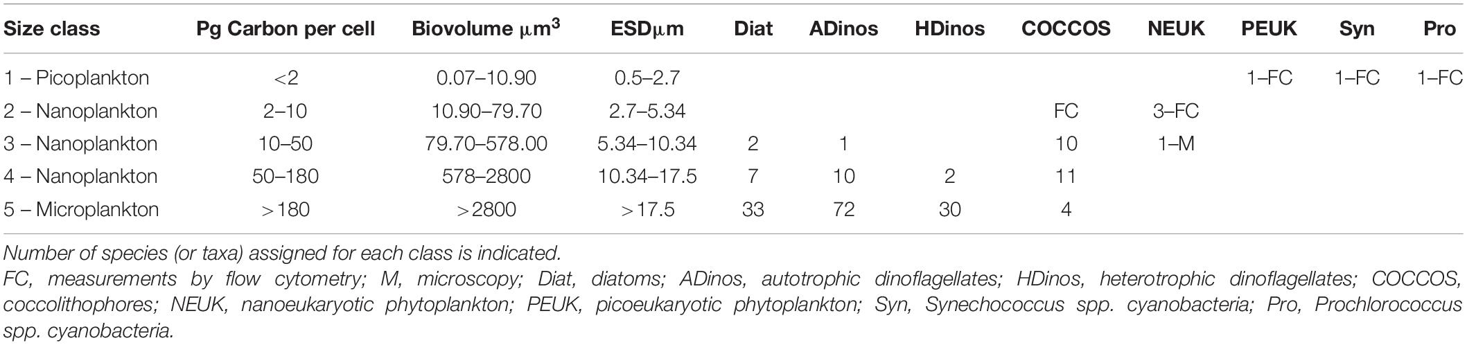
Table 1. List of the five plankton classes defined according to: Carbon per cell content, biovolume, and size as equivalent spherical diameter (ESD).

TABLE 2

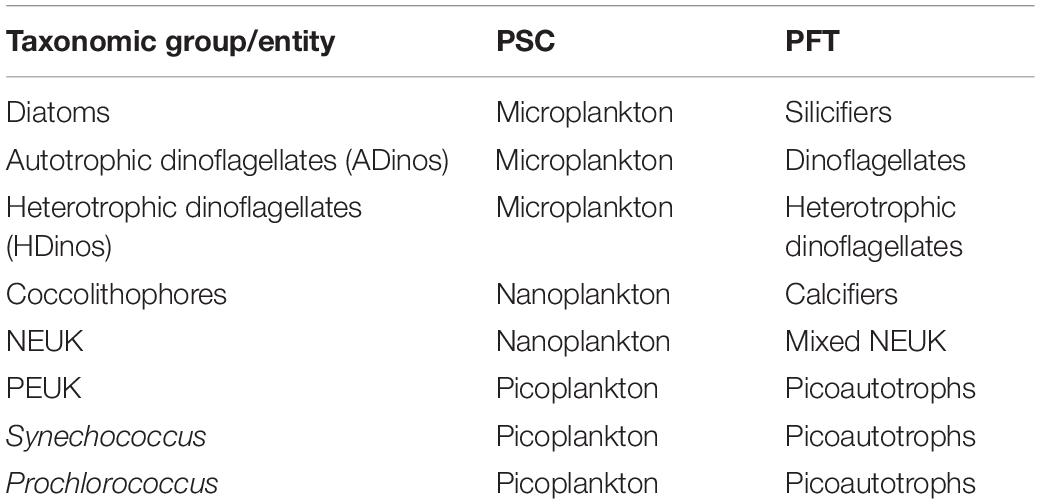
Table 2. Relation between taxonomic group or entity, phytoplankton size classes (PSCs), and phytoplankton functional groups (PFTs).

The upper limit for picoplankton is not agreed in the literature, varying between 2 μm (Jeffrey et al., 2011) and 3 μm (Buitenhuis et al., 2012), who note that the size range is a source of ambiguity for estimating carbon budget. By establishing 2.7 μm we are near the value indicated by Buitenhuis et al. (2012).

It should be stressed that diatoms and dinoflagellates have a wide variety of forms; hence, for any cell with a non-spherical shape, at least one of the dimensions is bigger than the ESD. For example, the smallest diatom species observed in this work, Cylindrotheca closterium, with a cell carbon content of 15 pg, and a biovolume of 200 μm³, has a rotational ellipsoid form, where the width is 2.8–5.5 μm and length 20–35 μm (Olenina et al., 2006). Hence, establishing the carbon class 4, with ESD from 10.3 to 17.5 μm is relevant to estimate the contribution of smaller diatoms and dinoflagellates.

Three-Component Model of Phytoplankton Size Class

The three-component model of PSCs of Brewin et al. (2010), was fitted to the Chla data as well as to the carbon data. The model estimates the fractional contribution of the three PSCs (micro-, nano-, and picoplankton), defined from the pigment content as a function of total Chla, as described above. The model has been successfully applied to widespread datasets (Brewin et al., 2015, 2017a) and to specific oceanic regions (Brotas et al., 2013; Brito et al., 2015; Brewin et al., 2017b; Corredor-Acosta et al., 2018). The model assumes that TChla derives from the sum of Chla from the three PSCs, and uses two exponential functions to calculate C_p,n (Chla of nano + picoplankton), and C_p (Chla from picoplankton), as a function of TChla (denoted C in the equations below), according to the following equations from Brewin et al. (2015):

$$C_{p,n}=C_{p,n}^m\left[1-exp\left(-\frac{D_{p,n}}{C_{p,n}^m}C\right)\right]$$

$$C_p=C_p^m\left[1-exp\left(-\frac{D_p}{C_p^m}C\right)\right]$$

$C_{\mathrm{p},\mathrm{n}}^m$ and $C_p^m$ are the asymptotic maximum values of Chla for the two size classes (<20 μm and <2 μm, respectively). The Chla concentration of nanophytoplankton (C_n) and micro-phytoplankton (C_m) are simply calculated as C_n = C_p,n−C_p and C_m = C−C_p,n.

D_p,n and D_p reflect the fraction contributed by each size class to TChla as TChla tends to zero, and they should take values in the range between 0 and 1 to ensure size-fractionated Chla does not increase faster than TChla. Also, D_p should never exceed D_p,n, as the fraction of cells <2 μm must obviously be smaller than the fraction of cells <20 μm.

Here, we also fitted the same set of equations to the carbon data, where in this case C becomes carbon, and the set of parameters ($C_{\mathrm{p,n}}^m$, $C_p^m$, D_p,n, and D_p) are with respect to carbon biomass.

Results

Nutrients and Mixed Layer Depth

The concentrations of nitrate + nitrite, phosphate and silicate, from surface to 200 m depth, as well as the depth of the mixed layer is illustrated in Figure 2. Concentration of nitrate + nitrite and phosphate in the surface were below quantification limits in most stations. MLD was from 50 to 11 m in the Northern hemisphere, reaching values higher than 90 m in the southern hemisphere (from latitudes 30 to 38° S), with a maximum value of 187 m at 36° S.

FIGURE 2

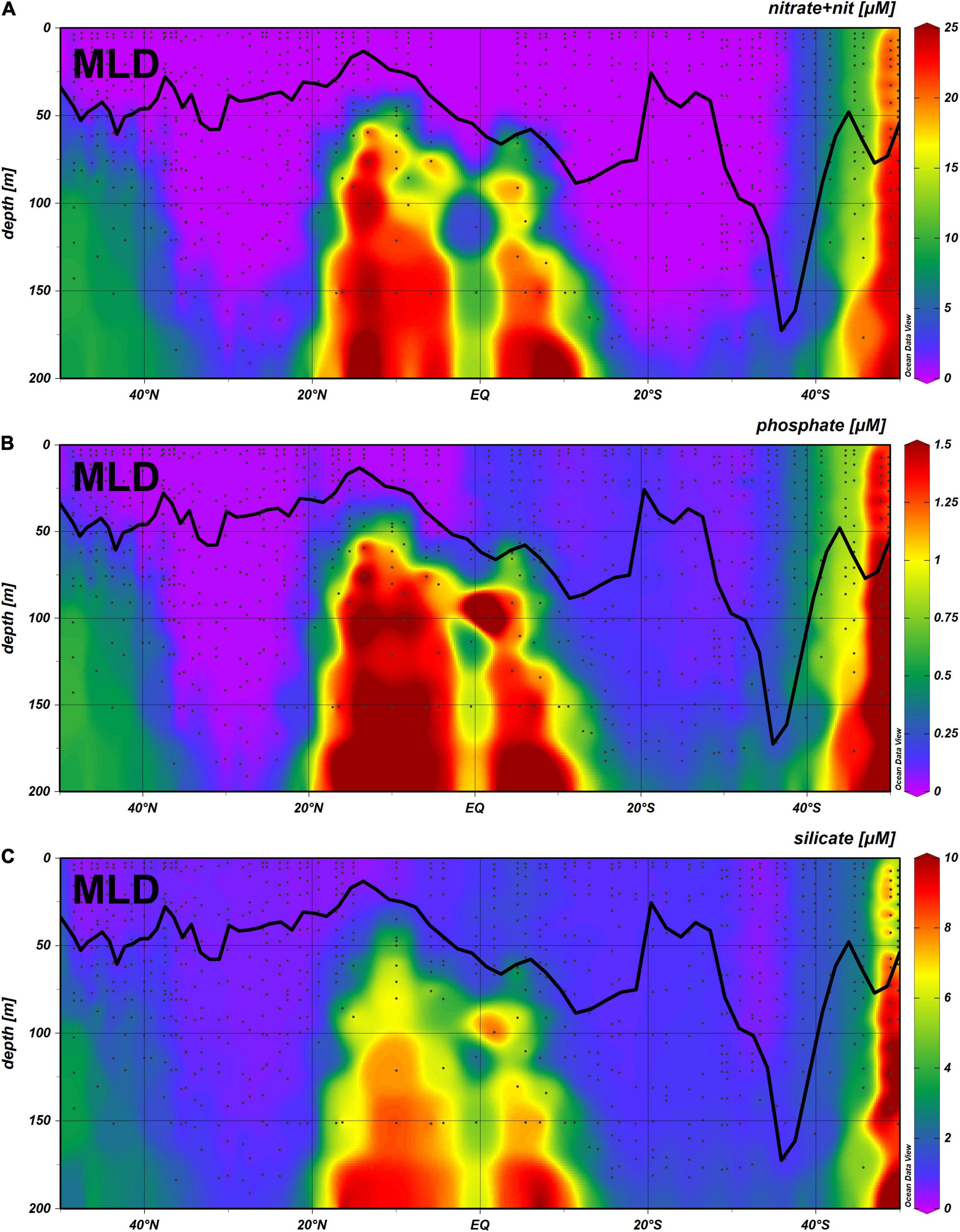
Figure 2. Concentration of nitrate + nitrite (A), phosphate (B) and silicate (C), from surface to 500 m depth, along the AMT25 transect, with the Mixed Layer Depth plotted along the transect.

High nutrient values throughout the water column up to the surface were present only south of 40° S. The low concentration of nutrients down to 200 m in the North Atlantic Gyre (NAG) and South Atlantic Gyre (SATL) is clearly visible.

Nitrate + nitrite values within the MLD were above quantification limit only in three distinct areas, within a narrow range of latitudes, namely from 50 to 44° N, from 0 to 8° S, and from 35 to 49° S. Values for silicate within the MLD were always above quantification limit, whereas for phosphate values were below quantification limit in NAG but not in SATL.

Phytoplankton Community Composition

Microscopy and Flow Cytometer Analysis

Using the cell carbon content allowed comparison of the biomass contribution of all phytoplankton classes/divisions in the Atlantic transect, considering both the cell counts done by microscopy and by FC. By microscopy, taxa from the following groups were enumerated: bacillaryophyceae (diatoms, 43 taxa), ADinos (84 taxa), HDinos (32), coccolithophores > 10 μm (25 taxa), filamentous cyanobacteria (5 taxa), prasinophyceae (7 taxa), and the haptophyte Phaeocystis spp. Taxa were identified at the species level, whenever possible. By flow cytometer, six groups were enumerated, Prochlorococcus spp., Synechococcus spp., picoeukaryotes (PEUK), coccolithophores <10 μm (COCCOS), cryptophytes (CRYPTO), and nanoeukaryotes (NEUK).

The relative abundance of the various phytoplankton groups, expressed in cell carbon content per volume is displayed in Figure 3, whereas the absolute values are detailed in Figure 4. There was a dominance of prokaryotic picoplankton groups throughout the latitudinal gradient, except for the stations located between 48–47° N and 48–49° S. The contribution of Prochlorococcus to total cell carbon m^–3 (Figure 4A) was higher than 50% from 43° N to 26.5° S, with the exception of the region influenced by the equatorial upwelling south of the equator (0° to 8° S); its biomass decreased sharply with decreasing temperatures (Figures 1, 3), south of 35° S. Synechococcus biomass increased in the Southern latitudes, and in the equatorial upwelling region (Figures 3, 4B). The group PEUK encompassed various taxa, poorly known; its biomass attained values above 5 mg carbon m^–3 only in a few stations of high northern and southern latitudes, as well as in the equatorial upwelling region, with values of 2–4 mg carbon m^–3.

FIGURE 3

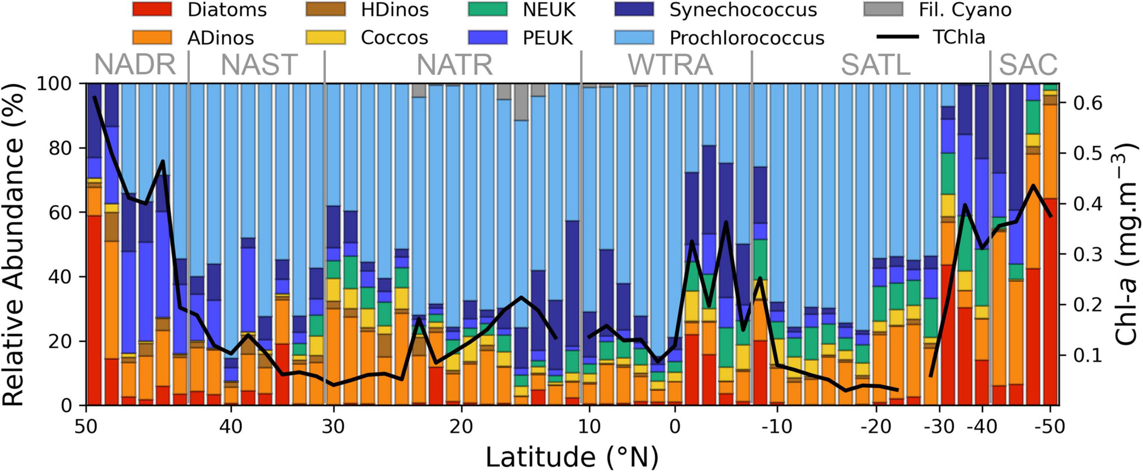
Figure 3. Relative abundance of major phytoplankton groups, enumerated by FC or microscopy and estimated in mg carbon m^–3, along the AMT transect (N-S), Chla value is also plotted. The correspondence between groups and size classes is given by the colour code: Picoplankton, blue tones; Nanoplankton, yellow and green; Microplankton, red and brown. Longhurst provinces are indicated. NADR, North Atlantic Drift; NAST, North Atlantic Subtropical Gyre; NATR, North Atlantic Tropical Gyre; WTRA, Western Tropical Atlantic; SATL, South Atlantic Gyre; SAC, South Atlantic Convergence.

FIGURE 4

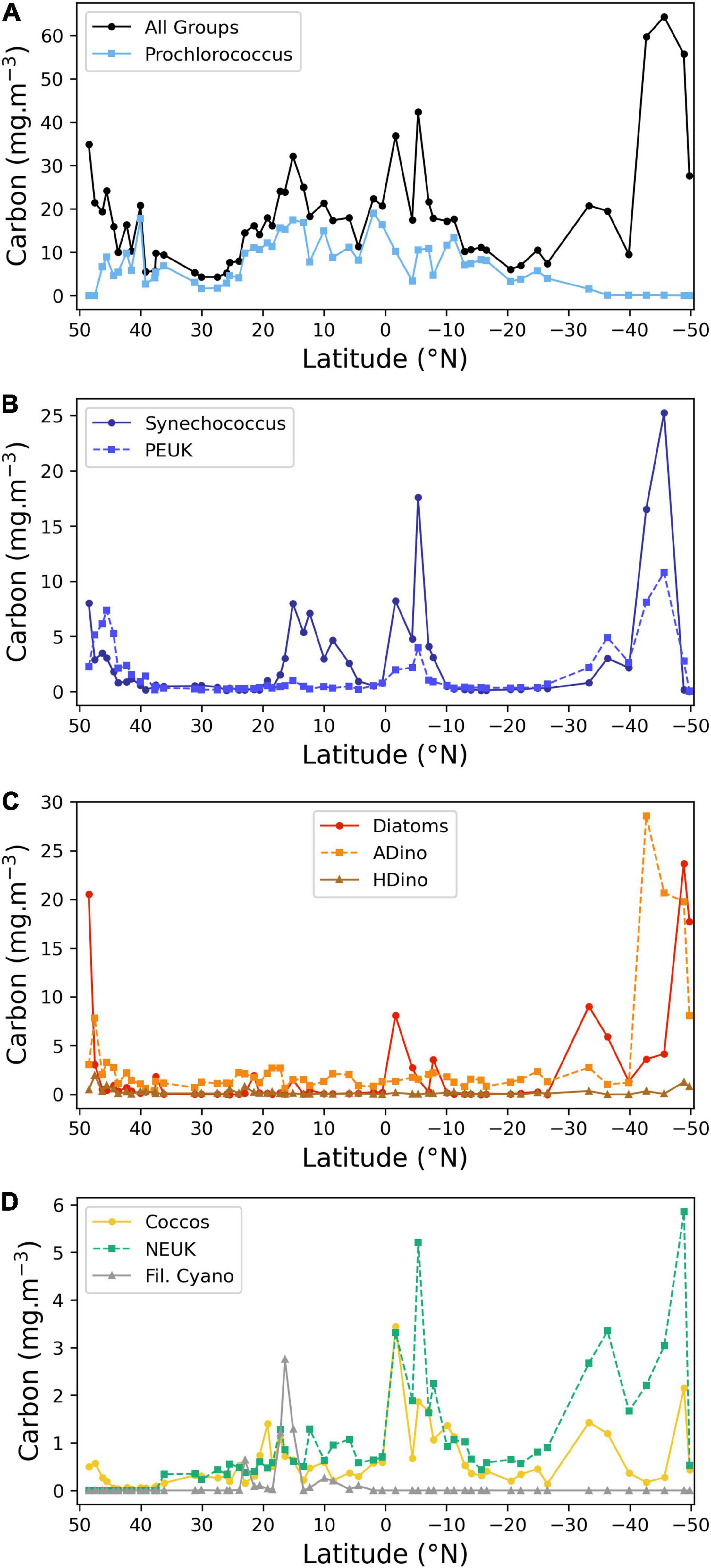
Figure 4. Latitudinal distribution of the carbon biomass (mg carbon m^–3) of the main phytoplankton groups, determined by FC or microscopy. (A) Total carbon of all groups and Prochlorococcus spp.; (B) Synechococcus spp. and picoeukaryotes (PEUK); (C) autotrophic and heterotrophic dinoflagellates and diatoms; (D) coccolithophores, other nanoplankton and filamentous cyanobacteria. Note different scales on Y-axes.

Diatoms were present at the majority of stations. High biomass values were found in the English Channel and southern latitudes, reaching a maximum value at most southern station (49° S), where the genus Pseudonitzschia and the large species Proboscia alata were dominant. Diatom biomass also increased between 1.7 and 8° S, due to the following taxa: Thalassiothrix, Rhizosolenia, Pseudonitzschia, and small pennate diatoms. Diazotrophic diatoms, belonging to the genus Hemiaulus, with Hemiaulus hauckii as the more abundant species, attained significant concentrations at latitude 15° N, near, but not coincident with the Trichodesmium peak.

Autotrophic and heterotrophic dinoflagellates are presented separately, as each group has very different ecological requirements. Autotrophic small unchained species were present at low abundance along the transect. From latitudes 45.6° to 41.5° N, the small toxic species Prorocentrum cordatum was abundant (from 0.8 to 2.4 × 10³ cells L^–1) In the South Atlantic, a sharp increase in ADinos occurred at 42.7° S, attaining 4 × 10⁴ cells L^–1, corresponding to 28.6 mg carbon m^–3, with a clear dominance of Oxytoxum spp. as well as the large-cell Karenia genus.

Heterotrophic dinoflagellates had very low abundance throughout the transect, with median and maximum values of 0.11 and 1.92 mg carbon m^–3, respectively. The maximum value was recorded at latitude 47.52° N, with the species Protoperidinium divergens.

The category “NEUK” (Figure 4D) includes cells counted under the microscope, namely Prasinophyceae and the genus Phaeocystis (haptophyta) as well as cells enumerated using the flow cytometer such as cryptophytes and other nanoeukaryotes. It should be underlined that cryptophytes and nanoeukaryotes enumerated by FC accounted, on average, for 99% of total carbon of the total “NEUK” category, and never less than 95%. This discrepancy is due to the difficulty in identifying small (<10 μm) flagellated cells by microscopy, as well as to the different order of magnitude of multiplying factors used in microscopy, 20 for a 50 mL Utermöhl chamber, versus 1250–2000 for the 500–800 μL of a sample analysed by FC, to a final result for both with cell abundance expressed per litre. Due to malfunctioning of the flow cytometer during the first week of the cruise, NEUK, CRYPTO, and COCCOS <10 μm diameter were not recorded in the northern latitudes. For this reason, the plot only displays “NEUK” from 37° N southwards, showing a biomass increase south of the equator and in the Southern Ocean.

Coccolithophores include cells identified and counted by microscopy (>10 μm diameter) and cells enumerated by FC (<10 μm diameter). The percentage of species with >10 μm diameter in relation to the total is higher than 20% in the majority of the transect, attaining a maximum of 93% at latitude 19.3° N, due to the species Umbilicosphaera cf sibogae, with cell diameters of 20–30 μm; the total coccolithophore biomass also increased in the equatorial upwelling and southern latitudes (>30° S), reaching a maximum at 1.7° S, due to high cell numbers of the same species. The species Emiliania huxleyi was present throughout the transect, confirming its ubiquity, peaking in 48.9° S.

Nitrogen fixing filamentous cyanobacteria, namely Oscillatoria, Planktothrix, and principally Trichodesmium were present between 30° N and 4° N, attaining values >1 mg carbon m^–3 between 15 and17° N, where MLD was shallower and surface nitrate + nitrite values negligible, but absent at all the other stations.

Phytoplankton Functional Types Dominance on the Different Oceanic Regions

The definition of Phytoplankton Functional Types (PFT) varies depending on the aim of the research, hence, there is no straightforward correspondence to taxonomical classes/divisions (Le Quéré et al., 2005). We were able to quantify the following functional groups, directly from FC and microscope counting: picoautotrophs, calcifiers (coccolithophores), silicifiers (diatoms), diazotrophs (filamentous cyanobacteria and symbiontic diatoms), ADinos, HDinos and mixed nanoeukaryotes (which exclude coccolithophores, and include cryptophytes and mixed NEUK counted using FC as well as prasinophytes and Phaeocystis spp. enumerated by microscopy), see Table 2.

The regions along the transect where each PFT presented positive or negative anomalies in relation to the mean are depicted in Figure 5. For each group, the value plotted represents the value of cells in mg carbon m^–3 for each sampling station divided by the average of that group for all stations, and normalized to the maximum value for that group. All groups registered lower biomass in the northern (39° N – 23° N) and southern (13° S – 27° S) gyres. Diazotrophs showed a sharp positive anomaly from 17 to 15° N. In higher latitudes and in equatorial region south of equator, all other groups presented positive anomalies. Table 3, displays the average value of carbon biomass per region. The overall average value was 18 mg carbon m^–3, within a range from a minimum of 4 in the Northern gyre (NAST) to a maximum of 64 mg carbon m^–3 in South Atlantic Convergence (SAC). Table 3 also shows that the maximum number of taxa observed in the regions with biomass growth, which was similar, between 57 and 68, whereas the regions of the northern and southern gyres registered a maximum of 45 and 48.

FIGURE 5

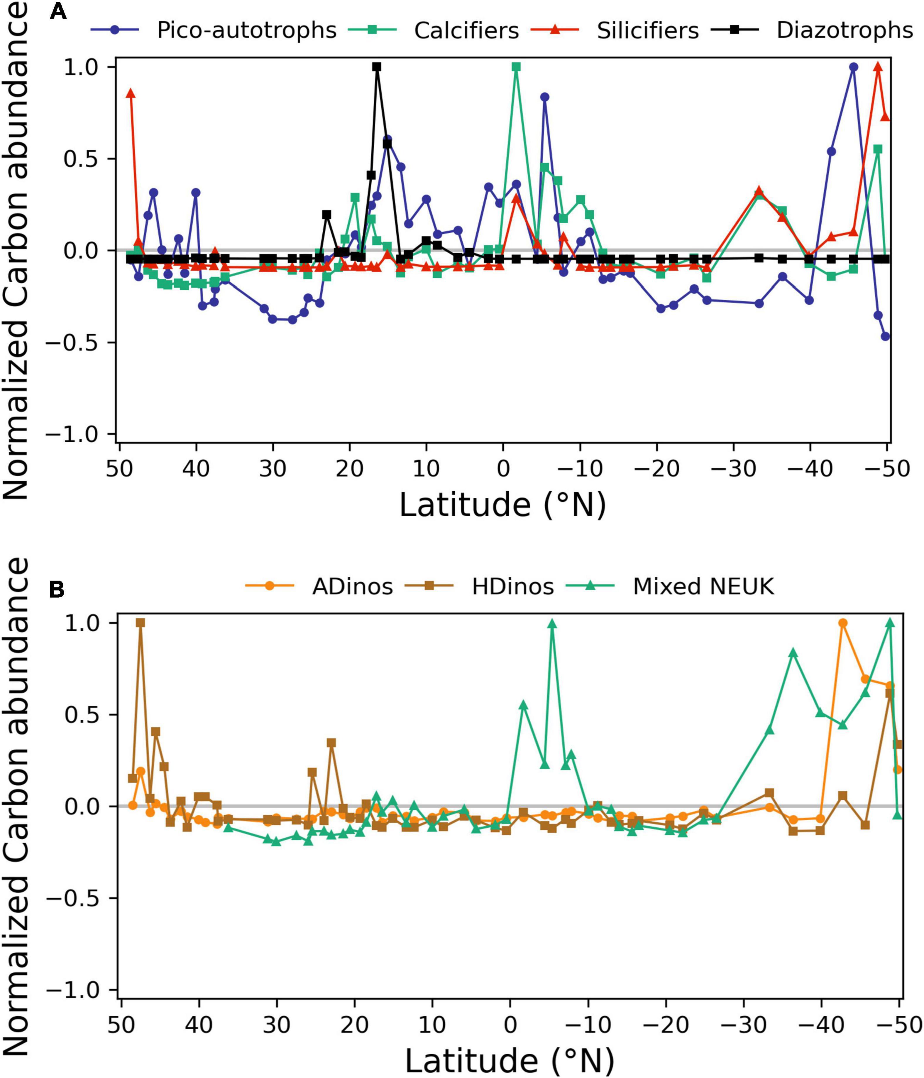
Figure 5. Normalised carbon abundance distribution (mg carbon m^–3) of phytoplankton functional types (PFTs) along the transect, determined by FC or microscopy. (A) Picoautotrophs, calcifiers, silicifiers, and diazotrophs; (B) autotrophic dinoflagellates (ADinos), heterotrophic dinoflagellates (HDinos), and mixed nanoeukaryotes (NEUK). Positive and negative anomalies observed for each PFT and normalised to its maximum value.

TABLE 3

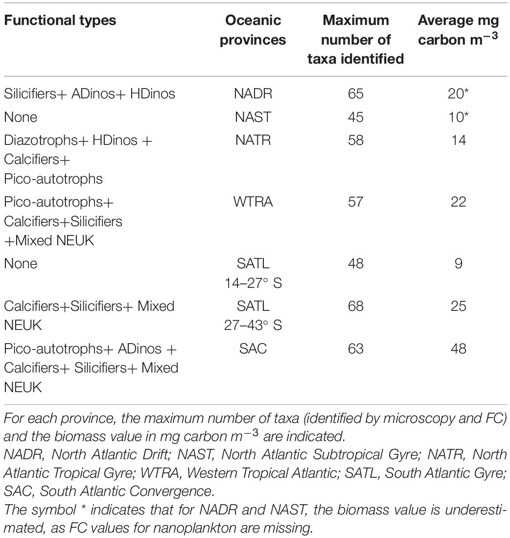
Table 3. Phytoplankton functional types contributing to biomass increase along the transect.

The dynamics of picoautotrophs, depicted in Figure 5, can be complemented with results from Figure 4: Prochlorococcus were the dominant taxa in both gyres, a shift from Prochlorococcus to Synechococcus occurred near more nutrient-rich or colder regions, and finally at highest latitudes, PEUK responded positively to nutrient increase.

As showed in Figure 2, the nutrients concentration in surface waters, were very low (often below quantification limit), thus preventing statistical analyses. The exception was the concentration of silicate, where a significant correlation was found with diatom carbon cell abundance (r² = 0.49, p < 0.05; model II regression).

The temperature along the transect (Figure 1) spanned from 5°C in the two southern stations, to 29°C at 12° N, being higher than 20°C in the large region from 40° N to 26° S. It should be highlighted that whilst in the northern hemisphere this study corresponds to autumn, in the southern hemisphere represents spring. A further analysis of the different species dominance in these regions is beyond the scope of this work, and will be done in the future.

Size Class Abundances Estimated According to the Pigment Approach and Cell Carbon Approach

Figure 6 illustrates the distribution of three size classes (pico-, nano-, and microplankton) according to both the pigment approach and the cell/carbon approach. Figure 6A shows the value of mg Chla m^–3 allocated to each size class, as well as the TChla concentration along the transect. The TChla median value is 0.13 mg m^–3, with higher values in the northern and southern stations, and between 0 and 8° S. Along the transect, higher values of TChla were due to higher Chla values estimated for all the 3 size classes. The sharp increase of nanoplankton Chla occurring north of latitude 44° N, is not possible to characterize in detail, due to the lack of FC results.

FIGURE 6

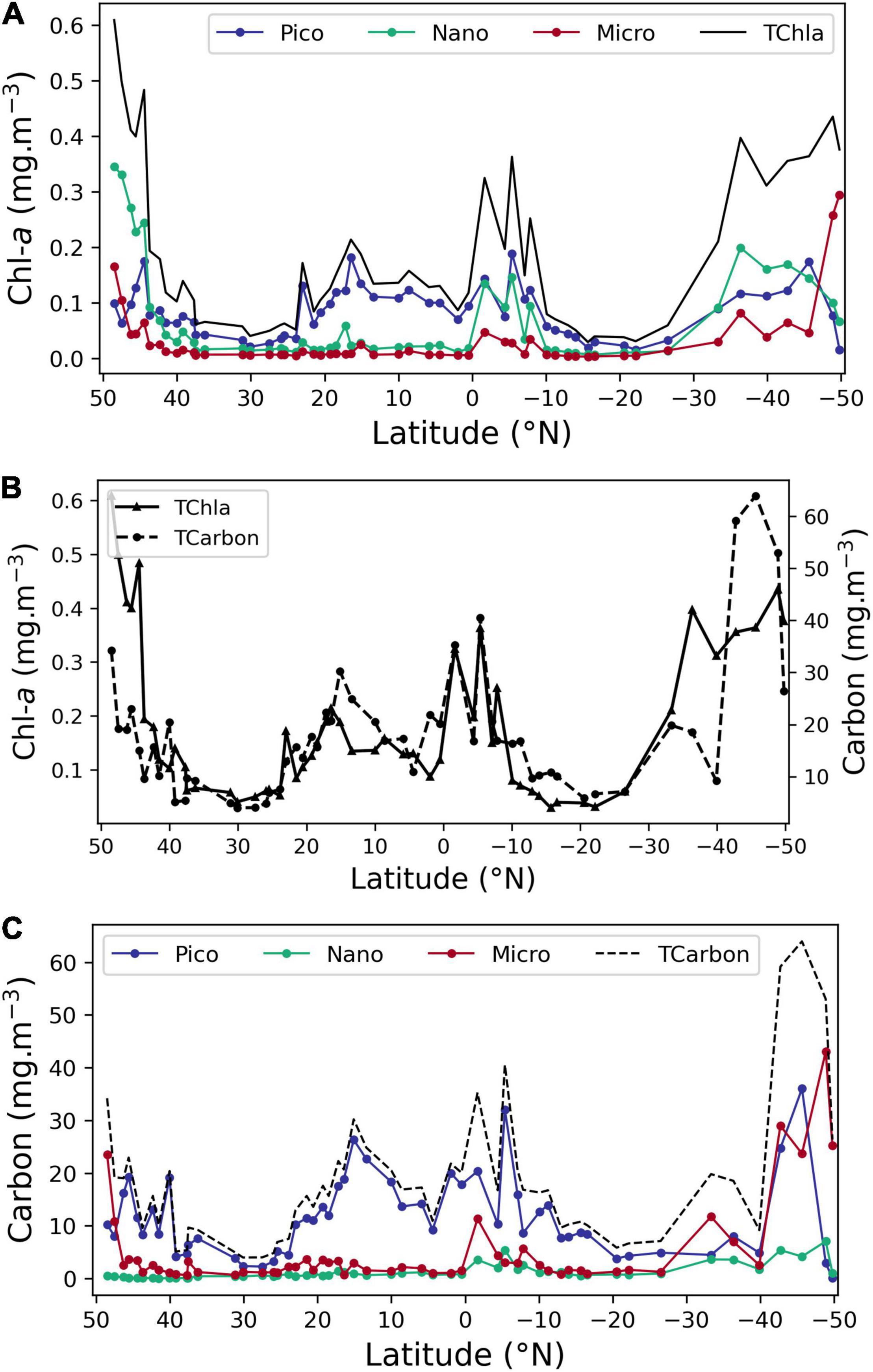
Figure 6. Distribution of size classes pico-, nano-, and microplankton obtained by pigment (determined by pigments’ concentration) and carbon approaches (determined by cell enumeration). (A) Chla concentration (mg Chla m^–3) observed along the transect using the pigment approach for the pico-, nano-, and microplankton, as well as Total Chla. (B) Total Chla and total carbon (mg m^–3); (C) mg carbon m^–3 for 3 size classes pico-, nano-, and microplankton, as well as total carbon. Note that total carbon values in (B) and nano-values in (C) north of 37° N are underestimated due to the lack of NEUK FC data.

Figure 6B shows total carbon (mg carbon m^–3) and TChla (mg Chla m^–3) along the transect; although there is a general agreement of the two, there are notable differences in higher latitudes. At northern stations, this mismatch is undoubtedly due to the lack of flow cytometer cell values for NEUK, CRYPTO, and COCCOS <10 μm diameter from 49 to 37° N, implying that these taxa must be an important component of the phytoplankton community in this region. In fact, cell counts by microscopy registered high values for prasinophytes, coccolithophores and for the genus Phaeocystis in this region, justifying the assumption that FC counts for the above groups would also have showed high biomass levels. In the Southern latitudes, the community is dominated by diatoms, with ESD from 30 to 100 μm and by ADinos, with ESD above 20 μm. The linear increase in diameter corresponds to an exponential increase in cell volume and consequently in cell carbon content, which may be biased by the volume-carbon equations used, as it would be expected that larger cells have a less dense cell content, and, hence, less carbon per unit volume.

Figure 6C shows the distribution of the phytoplankton community, expressed in mg carbon m^–3, and also divided into three size classes, where each class was established according to the carbon content per cell (Table 1). Carbon nano class includes classes 2, 3, and 4 of Table 1, so that the carbon classes are equivalent to the pico-, nano-, and microplankton classification of the pigment approach. The most abundant was the smallest class, corresponding to organisms with less than 2 pg carbon cell^–1, i.e., picoplanktonic organisms, followed by the largest class, organisms with more than 180 pg carbon cell^–1, corresponding to cells with a diameter of 17.5 μm or more. As referred to above, micro carbon class (larger cells) stands out because of the dominance of large diatom and dinoflagellate species at high latitude which make up the biomass peaks. The lower contribution of nanoplankton class to total carbon, in relation to the results from the pigments approach is observed by comparing Figures 6B,C.

The carbon nano class, corresponding to organisms with ESD between 2.7 and 17.5 μm, had low biomass throughout the latitudinal transect (Figure 6C). Within this cell size range, the contribution of three intermediate carbon classes was compared (data not shown): class 2, which is estimated exclusively by FC, presented the highest biomass, with a median value of 80% of the total carbon nano class.

As neither oceanic Chla concentration nor species cell size follow a normal distribution, in order to perform a statistical analysis on the two size class approaches, carbon mg m^–3 and Chla mg m^–3, data were log₁₀ transformed. Type II regression analyses were performed for the total value of Chla and carbon values along the transect, as well as for matching size classes estimated by both approaches. The regression analysis was computed as log₁₀Carbon = m.log₁₀Chla + b. The equation coefficients and correlation values for the relationships with significant Pearson correlation values are shown in Table 4. Chla-microplankton was matched with carbon size class 5 (cells with >180 pg carbon cell^–1) and also with the sum of carbon classes 4 and 5, corresponding to cells with >50 pg carbon cell^–1 and ESD >10 μm, so as to account for the strong shape variability of diatoms and dinoflagellates. Both correlations gave the same equation coefficients and r² value. Concomitantly, Chla-nanoplankton was matched with carbon size classes 2 (cells 2–10 pg carbon cell^–1), the sum of classes 2 and 3 (cells 2–50 pg carbon cell^–1) and the sum of classes 2, 3, and 4, corresponding to cells from 2 to 180 pg carbon cell^–1, with a range of ESD from 2.7 to 17.5 μm. A significant correlation was obtained for the smallest cells and for the sum of the three carbon size classes defined within nanoplankton. This result is not surprising, due to the methodological issues regarding identification and enumeration of cells within an ESD range of 10–17.5 μm, already discussed. Moreover, it reflects the dominance of small species in nanoplankton size class.

TABLE 4

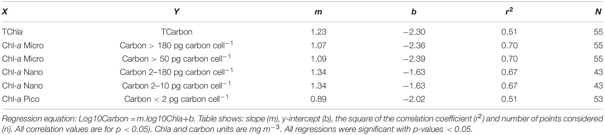
Table 4. Results of linear regression Type II of log10-transformed carbon and log10-transformed Chla for the total data set, as well as for the matching size classes estimated by the pigment or carbon approaches.

Three Component Model of Size Classes Applied to Chla and Carbon Data

The three-component size class model of Brewin et al. (2010) was applied to TChla and, for the first time, also to TCarbon (Figure 7).

FIGURE 7

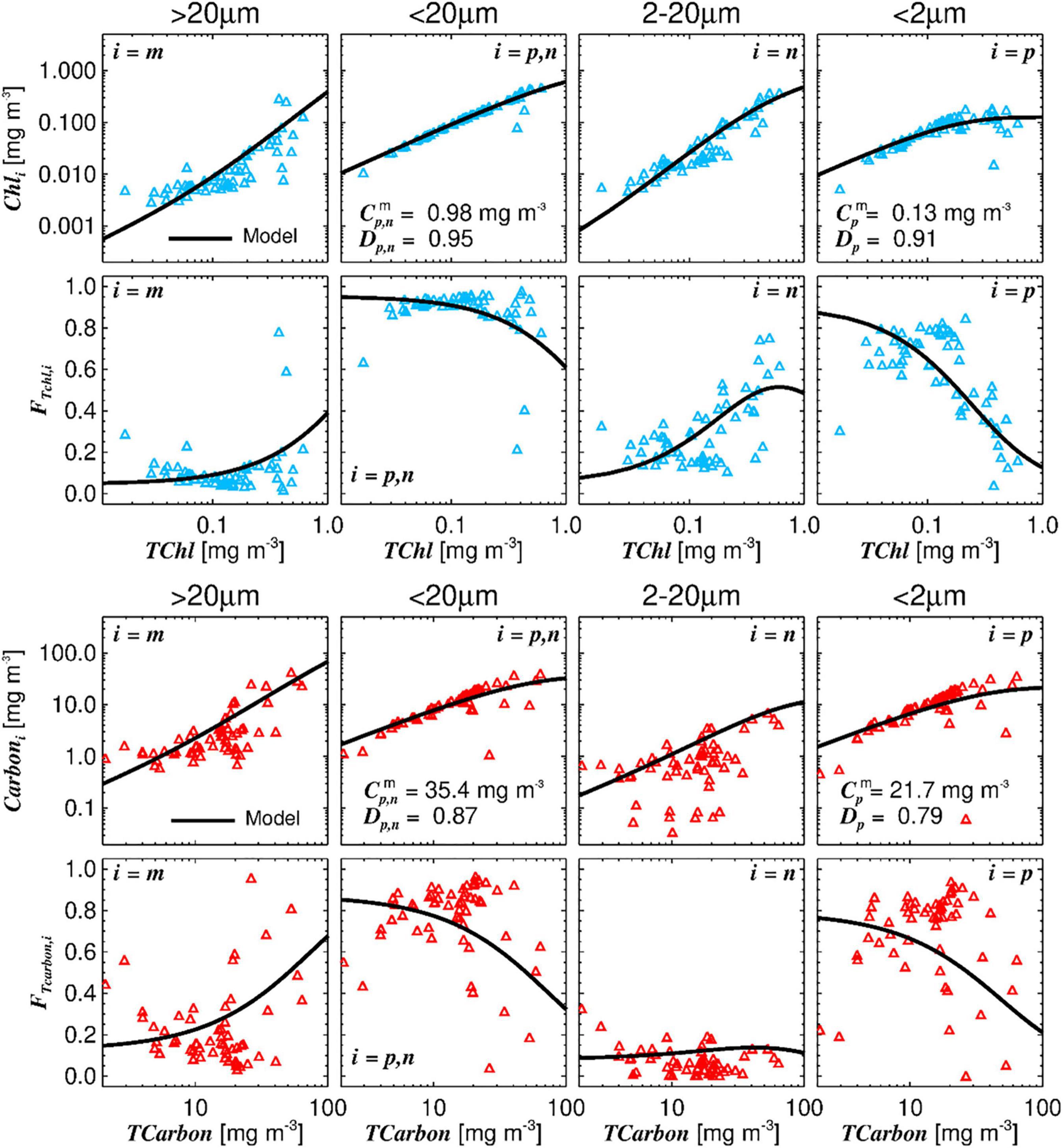
Figure 7. Three component model applied to TChla and TCarbon. Top row: the three component model fitted to chlorophyll-a values associated with the different size classes: microplankton (Cm), picoplankton, and nanoplankton combined (Cp,n), nanoplankton by itself (Cn), and picoplankton by itself (Cp); Dp,n and Dp reflect the fraction contributed by size-class pico and pico+nano to TChla as TChla tends to zero. Second row: the size-specific fractional contributions of microplankton (Fm), nano+picoplankton (Fn,p), nanoplankton (Fn), and picoplankton (Fp), plotted according to the model as a function of total Chla. Third row: the model applied to TCarbon values (assessed by cell enumeration converted into carbon) associated with class 5 (im), classes 2, 3, 4 (in), and class 1 (ip) (see Table 1). Fourth row: size-specific fractional contributions to Fm, Fn,p, Fn, Fp, obtained from the carbon dataset.

Total chlorophyll-a is plotted in the top six graphs (blue markers), and TCarbon on the six bottom graphs (red markers). The general pattern of the model fitted to TCarbon is in accordance with the one obtained with TChla. With the exception of the graph showing the fraction of nanoplankton as a function of TChla (third graph second row) or TCarbon (third graph fourth row), which is due to the methodological issues regarding the estimation of nanoplankton cells mentioned above. The ratio of the parameters ($C_{\mathrm{p,n}}^m$ and $C_p^m$) obtained for TChla and TCarbon give a value for Carbon:Chla of 170 for picoplankton and 36 for nano plus picoplankton classes, which are reasonable, as picoplankton cells have higher carbon content per μm³ cell volume. The overall median Carbon:Chla ratio estimated from the in situ data was 112, presenting a wide variability, most pronounced in microplankton fraction.

However, it should be noted that $C_{\mathrm{p,n}}^m$ and $C_p^m$ parameters have a high uncertainty as the phytoplankton biomass concentrations along the AMT are low (TChla maximum was 0.7 mg m^–3 and TCarbon maximum was 70 mg m^–3). The D_p,n and D_p parameters are slightly higher for TChla than for TCarbon, but both highlight the dominance of picoplankton at low total biomass.

Discussion

Complementarity and Knowledge Gaps Between the Pigment and Carbon Approaches

This work has showed that both approaches give a similar general picture in terms of biomass size distribution and composition in the Atlantic, although with poorer results for the nanoplankton fraction.

Microplankton size class in the pigment approach is estimated by only two diagnostic pigments: fucoxanthin, the primary pigment for diatoms, and peridinin, the primary pigment for dinoflagellates. Brewin et al. (2017a) further split the microplankton class into the fraction of diatoms to total Chla (F_diat) and also the fraction for dinoflagellates to total Chla (F_dino). The same computation was applied in this study. The total diatom carbon biomass showed a significant correlation with F_diat (r² = 0.70, n = 56, p < 0.05). However, no correlation was found for F_dino and ADinos; and this can be explained because ADinos attained their maximum values in the three southern stations (42.72–49.78° S, Figure 4C), due to high cell abundances of Karenia and Oxytoxum spp. The genus Karenia does not contain peridinin (Roy et al., 2011), hence the lack of correlation between carbon values and Chla (F_dino). This observation aims to provide an alert to the diversity of pigment composition found in some taxonomic groups, which might be considered flaws in the pigment approach for some regions/occasions. However, disadvantages of microscopy should also be remembered, namely, the stronger dependence of the operator expertise for species identification, as well as the longer time consuming of microscopy in comparison with pigments analysis by HPLC.

Additionally, our results, whilst supporting the strength of the chemotaxonomic approach, also show that the absence of an association between dinoflagellates and F_dino, evidences the fragility of the pigment approach when applied regionally, due to the variability of pigment composition in some taxonomic classes. This is mostly relevant for the division Dinophyta, with five different types, and for class Coccolithophyceae within the division Haptophyta, with six different types (Roy et al., 2011).

The Uitz et al. (2006) equation to estimate nanoplankton uses three diagnostic pigments: 19′hexanoyloxyfucoxanthin (HF), 19′butonoyloxyfucoxanthin (BF), and alloxanthin; the first two are a proxy for coccolithophores and the third for cryptophytes. However, these three pigments can be present in other divisions/classes from micro- and picoplankton, for example, dinoflagellates (Dinos type 2 for HF and BF and Dinos type 4 for alloxanthin) as well as small flagellates belonging to the PEUK (Roy et al., 2011). In fact, the group PEUK comprises classes with high molecular phylogenetic diversity and multiple ecological roles (Worden and Not, 2008). Our results gave significant correlations between both HF and BF with coccolithophore carbon biomass, but also with PEUK, suggesting the existence of small Prymnesiophyceae and Pelagophyceae in PEUK.

This work showed that the pigment approach overestimated the nanoplankton fraction compared to enumerating methods. The nanoplankton fraction is especially diverse in terms of taxonomic classes, and consequently pigment composition. Cell identification and counting methods are probably underestimating nanoplankton, in particular for the size class with ESD 5–10 μm. Hence, it is not surprising to find that the nanoplankton fraction bears poorer results in terms of comparison of carbon concentration, to the pigment approach. The use of diagnostic pigments to determine PSC relative abundance still constitutes a debate in recent literature, where conflicting conclusions can be found. Brewin et al. (2014) used a large database from AMT cruises (ca 460 samples from 1996 to 1998) to compare size fractionated filtration with HPLC pigment quantification and found that diagnostic pigment approach (DPA) overestimated nanoplankton fraction and underestimated picoplankton. Likewise, Dutkiewicz et al. (2020), also focusing on an early AMT data set concluded that allocated Chla for picoplankton size class in the pigment approach is potentially slightly too low and the nano-size class too high, suggesting that the satellite product derived from this division might not be exact. In contrast, Chase et al. (2020), studying samples from the western North Atlantic showed that the DPA overestimated microplankton and picoplankton when compared to Imaging FlowCytobot (IFCB) data, and subsequently underestimated the contribution of nanoplankton to total biomass. These opposing findings might also be related to the studied regions, as Chase et al. (2020) study focus on the western North Atlantic Ocean, i.e., a meso-eutrophic region, whereas the vast majority of samples in Brewin et al. (2014) and Dutkiewicz et al. (2020) originated from oligotrophic and mesotrophic Atlantic regions. It is relevant here to quote the statement in Chase et al. (2020) that DPA involves the division of phytoplankton into distinct limits, whereas phytoplankton cell size displays a continuum. But it is also important to underline the common conclusion of the above three studies, reinforcing the need for complementary methodological approaches, to better characterize the taxa within each size class. We certainly agree with this statement, in particular regarding the nanoplankton fraction.

Size Classes Model for Carbon and Chlorophyll a

The model of Brewin et al. (2010) was applied to results obtained by both methods, showing for the first time that it can be applied to carbon data obtained from cell enumeration with success, albeit with a poorer fit to the nanoplankton fraction (Figure 7). The maximum value for Carbon:Chla obtained by applying Brewin et al. (2010) to both carbon and Chla estimates of size classes (Figure 7) was 170 for picoplankton and 36 for nano + picoplankton classes, these values are logical considering the relation between higher package effect and larger size cells (Bricaud et al., 2004).

From the estimation of F_diat, and the diatom carbon biomass, the average Carbon:Chla value of 60 was obtained, close to the value found by Sathyendranath et al. (2009) for diatoms in northwest Atlantic; however, a wide variation of this ratio was observed, which is related to the wide biovolume and shape variability of diatom cells.

Achieving a better understanding of the Carbon:Chla ratio for phytoplankton communities is paramount to our understanding of oceanic biogeochemical cycles, and as Sathyendranath et al. (2020) pointed out, estimating both Chla and carbon concentration is mandatory to improve our understanding of phytoplankton dynamics. Retrieval of size classes or functional groups by EO has been fundamentally based and validated with the information from photosynthetic pigments concentration (Brewin et al., 2021 and references herein). The results obtained in our work show a generally good agreement between the use of pigments and use of species/entities identification and enumeration converted into carbon biomass. Hence, this work can contribute to the capability of assessing phytoplankton carbon budgets by satellite remote sensing in future studies.

Phytoplankton Community Structure Along the Transect in the Atlantic

The AMT program started in 1995, comprising 30 cruises up to 2019, and provides an immense and extremely valuable set of scientific data (Rees et al., 2015; Aiken et al., 2016). During the first 10 AMTs (1995–2000), data on phytoplankton species was assessed and published as a database by Sal et al. (2013). Focusing only on the coccolithophore community, Poulton et al. (2017) published a comprehensive work based on four AMT cruises in Spring and Autumn between 2003 and 2005. Fileman et al. (2017) quantified flagellates, diatoms and dinoflagellates cells (without separating into species or genera) using FlowCAM on AMT10 (which occurred in 2000). During AMT22, phytoplankton cells were sorted and processed by a cell sorter flow cytometer, where each sample was up to 4 mL (Graff et al., 2015). Dutkiewicz et al. (2020) published their work on phytoplankton diversity with data from AMT 1 to 4 (1997–1997). Hence, to our knowledge, the classical phytoplankton species microscopy identification data presented in this article are the first from AMT after a 15 years gap.

The cell carbon approach allowed for the comparison of all groups, counted by microscopy or FC. The pattern of spatial distribution of total biomass of the phytoplankton community shows a strong relation with nutrient availability within the MLD, in accordance with the observations of Marañón et al. (2012) that resource availability and not temperature is the key factor explaining the relative success and abundance of different algal size classes.

The change observed in size class abundance is considerable. Higher carbon biomass values occurred in temperate/cold regions, attaining a maximum value of 65.5 mg carbon m^–3 in the SAC region (Figure 6C), where nutrients in surface waters reached a maximum, with nitrate + nitrite values of 20 μM. A significant biomass increase in all classes occurred in the equatorial upwelling (0–8° S), except for Diazotrophs and HDinos, due to their capability of atmospheric nitrogen fixing and heterotrophic behaviours, respectively. Very low values were registered in the Atlantic core gyres [defined following Polovina et al. (2008) as the regions where Chla was below 0.07 mg m^–3] with an average of 7.4 mg carbon m^–3, and ranging from 4.0 to 10. Fileman et al. (2017), who also converted cell abundances into carbon units using the equations of Menden-Deuer and Lessard (2000), reported a biomass range of 4–68 mg carbon m^–3, with the lowest values recorded in the gyres and maximum value in temperate regions, very similar to our results. However, Fileman et al. (2017) concluded that the microplankton size fraction (which included diatoms and dinoflagellates) comprised of only a very low proportion (1–15%) of total phytoplankton biomass, whereas our results indicate percentages >50% in most of north and southern Atlantic stations, reaching 94% at latitude of 49.78° S; we think that this difference is due by the higher detail of our measurements.

The community composition results were consistent with the general pattern reported in AMT cruises 1, 3, 5, and 7 (which occurred in boreal autumn/austral spring), with higher abundance and diversity of diatom and dinoflagellate species at higher latitudes and reduced numbers of cells, with ESD >20 μm in the Atlantic gyres. Marañón et al. (2007) (with a data set including the 1996 AMT cruise), had reported as well the dominance of larger phytoplankton in nutrient-rich waters. Similarly, Tilstone et al. (2017), using size fractionated filtration in five AMT cruises, registered higher microplankton production fraction in the SAC and Western Tropical Atlantic (WTRA) provinces. However, our results also indicate that there is not a shift between size classes, in absolute values, as all carbon size classes showed a positive and significative increase with higher TCarbon values (Figure 8), meaning that taxa from all sizes respond positively to nutrient increase. This finding is in accordance with Yentsch and Phinney (1989), who postulated that cell size structure in eutrophic waters is modified by adding larger cells without any apparent loss of the small-sized cells, and with Brotas et al. (2013) who suggested that all size classes are more abundant in more productive areas along a trophic gradient in the eastern Atlantic. Additionally, the ubiquitous survival of picoplankton in all oceanic environments is explained by Dutkiewicz et al. (2020) due to their capacity of steady state survival with minimum values of resources.

FIGURE 8

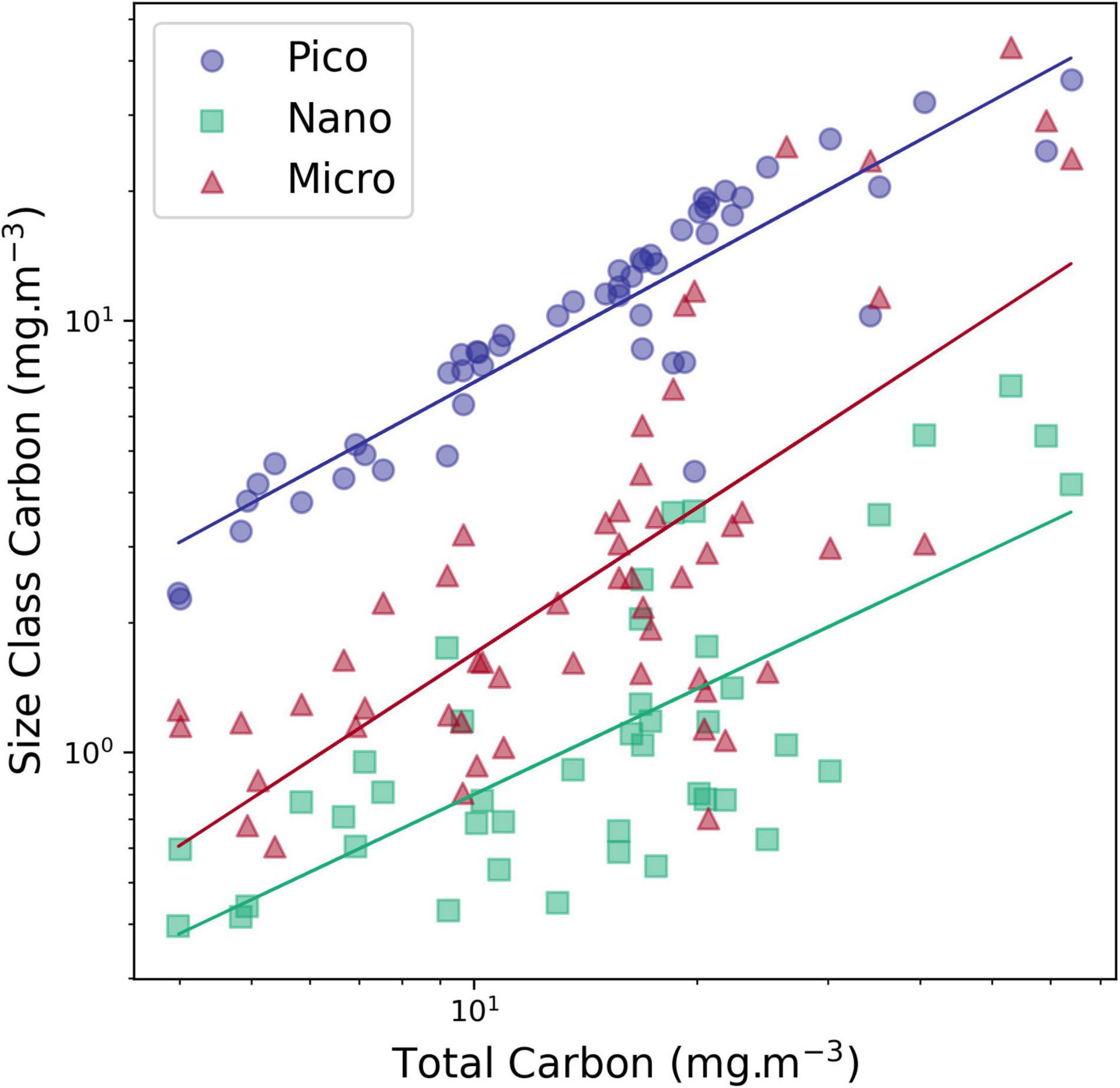
Figure 8. Carbon concentration of each size class versus total carbon concentration (determined by FCor microscopy). picoplankton carbon (Pico Carbon, <2 pg carbon cell^–1), nanoplankton, sum of carbon sizes 2, 3 and 4 (>2 <180 pgC cell^–1) and microplankton carbon (Micro > 180 Carbon, >180 pgC cell^–1). The correlation between each size class and TCarbon was significant (p > 0.01).

As mentioned in section “Introduction,” AMT programme delivers ground-truth information for satellite validation, hence, it is worthwhile in the present work to discuss the main features concerning the distribution of phytoplankton groups along the transect, as this information will likely be relevant for future works. The diatom species reaching a concentration of 1 mg carbon m^–3 per station, or above, had ESD between 30 and 100 μm, and 30% of them had a carbon content >1000 pg carbon cell^–1 (Supplementary Table 1). The sharp biomass peaks observed are always due to the presence of these larger cells. Smaller diatom species peak at stations from NADR, NATR, and SATL (NADR, North Atlantic Drift; NATR, North Atlantic Tropical Gyral; and SATL, South Atlantic Gyre), but always with values below 0.8 mg carbon m^–3. The distinction made in this work (in accordance with Sal et al., 2013), between autotrophic and heterotrophic (non-pigmented) dinoflagellates showed that HDinos were always present in very low abundance throughout the transect, but increased where diatoms were abundant, mostly through the dominance of five different Protoperidinium species (Figure 5B). This finding is in accordance with Sherr and Sherr (2007), who indicated that HDinos, ubiquitous in marine environments, seem to be able to survive at low food abundance, preying on diatoms, giving the example of Protoperidinium as a diatom predator. Concerning coccolithophores, the complementary enumeration in FC and microscopy was important to find out that the biomass of sizes within coccolithophores <10 and >10 μm is equivalent. The presence of E. huxleyi in all provinces with a distinct peak in the Southern temperate region was also observed by Poulton et al. (2017), on AMT14, who also concluded that coccolithophore cell numbers were highest in temperate waters. Filamentous cyanobacteria counts were not included in the size classes results (Figures 6, 8), as they are not accounted for in the microplankton fraction in the pigment approach; but their abundance is shown in Figures 3–5. It should be noted that diazotroph functional types include both filamentous cyanobacteria and diatoms with endosymbiotic cyanobacteria (which were present only at very low abundance). Filamentous cyanobacteria, with Trichodesmium being by far the most abundant genus, showed a distinct peak in the North Tropical Gyre. Previous northern hemisphere Autumn AMT cruises (i.e., AMT 1, 3, 5, and 7) reported maximum values between 9° and 20° N (Sal et al., 2013). Schlosser et al. (2013) also observed Trichodesmium maxima in this region, justifying it with a selective advantage for diazotrophic organisms in inorganic nitrogen depleted zones; moreover, these authors showed that activity of diazotrophs can in turn be controlled by the availability of other potentially limiting nutrients, including phosphorus (P) and iron (Fe).

Currently, PFT products are available through the CMEMS, using the approach of Xi et al. (2020). These authors used nine reflectance bands and a large and widespread diagnostic pigment database, defining six PFTs: diatoms, haptophytes, dinoflagellates, green algae, Prochlorococcus, and Synechococcus-like cyanobacteria (SLC). The relative dominance of PFTs they estimated for October (their Figure 12) can be compared with our results. The dominance of SLC in the gyres and WTRA and the dominance of Prochlorococcus does not correspond to our observations, agreeing with their own conclusion of a low performance for these two PFTs. The dominance of diatoms off the Patagonian coast is in agreement with our results, but not the dominance of haptophytes in temperate regions. Therefore, we would argue that there is still a great need for ground-truth validation of EO-based PFT retrievals.

The roadmap for a future successful discrimination of PFTs, lies in a multi-disciplinary approach which includes in situ measurements of phytoplankton groups (with an array of existing methodologies) and corresponding optical properties, observable by satellites (Bracher et al., 2017). Our work is a contribution to this goal, by providing results for the whole phytoplankton community in the Atlantic.

Conclusion

This work showed a good agreement between complementary assessments of phytoplankton structure, the widespread chemotaxonomic approach and the less used, more time consuming cell carbon approach. Using a varied set of data, collected along a transect in the Atlantic Ocean, from 50° N to 50° S, covering a wide range of oceanic provinces, allowed us to quantify phytoplankton taxonomic groups, and discuss their classification within a size class and functional types framework.

We applied, for the first time, the Brewin et al. (2010) model to in situ carbon data to assess phytoplankton size structure. The results obtained encourage the application of this model to cell carbon data, hence, establishing the link between PSC assessment by EO, and carbon.

Additionally, this study presents a comprehensive assessment of all phytoplankton groups in the Atlantic ocean, contributing to a better knowledge of phytoplankton community, providing biomass values for the various regions, as well as the number of taxa present, whilst identifying knowledge gaps, namely the composition of the picoeukaryote and nanoplankton fractions.

Relevant aspects to be considered in the future have also been pointed out by this work: notably regarding the nanoplankton fraction, which is overestimated by the pigment approach, and poorly evaluated by the combination of microscopy and FC. Nonetheless, the correspondence of nanoplankton measured by FC only and the nanoplankton in the pigment approach, validates the use of FC to quantify nanoplankton cells. Our results also evidence the importance of enumerating coccolithophores with ESD >10 μm, as the percentage of species with this dimension were at least 40% of the total coccolithophores concentration.

Data Availability Statement

The original contributions presented in the study are included in the article/Supplementary Material, further inquiries can be directed to the corresponding author.

Author Contributions

All authors contributed to the conceptual development of the manuscript. GT, RB, and CB contributed to cruise participation. RA contributed to HPLC pigment analysis. VV contributed to microscope identification and enumeration. EW contributed to nutrient analysis. AF contributed to figures and statistics. All authors contributed to manuscript revision, read, and approved the submitted version.

Funding

VB received a sabbatical grant from FCT (SFRH/BSAB/142981/2018). This work received funding from the European Union’s Horizon 2020 Research and Innovation Programme under grant agreement n° 810139 Project Portugal Twinning for Innovation and Excellence in Marine Science and Earth Observation – PORTWIMS. It also received support by national funds through FCT – Fundação IP, under the project UIDB/04292/2020. This work was also a contribution to ESA project Ocean Colour Climate Change Initiative, and Interreg Project Innovation in the Framework of the Atlantic Deep Ocean (iFADO). RB was supported by a UKRI Future Leader Fellowship (MR/V022792/1).

Conflict of Interest

The authors declare that the research was conducted in the absence of any commercial or financial relationships that could be construed as a potential conflict of interest.

Publisher’s Note

All claims expressed in this article are solely those of the authors and do not necessarily represent those of their affiliated organizations, or those of the publisher, the editors and the reviewers. Any product that may be evaluated in this article, or claim that may be made by its manufacturer, is not guaranteed or endorsed by the publisher.

Acknowledgments

This is contribution number 360 of the AMT programme. The Atlantic Meridional Transect is funded by the UK Natural Environment Research Council through its National Capability Long-term Single Centre Science Programme, Climate Linked Atlantic Sector Science (grant number NE/R015953/1). This study contributes to the international IMBeR project. We thank the officers and crew of the British Antarctic Survey vessel James Clark Ross. We are indebted to NEODAAS for processing the satellite imagery, we would like to thank Daniel Clewley for providing Figure 1, and we also acknowledge John Stephens for providing us the MLD data for the AMT25. We are also indebted to the three reviewers who improved the manuscript.

Supplementary Material

The Supplementary Material for this article can be found online at: https://www.frontiersin.org/articles/10.3389/fmars.2021.682621/full#supplementary-material

Supplementary Table 1 | List of species found and their abundances per sampling station (cell abundances determined by microscopy, and expressed in carbon). The codes of column A are the same as indicated by Sal et al. (2013).

Footnotes

1. ^ www.neodaas.ac.uk
2. ^ https://marine.copernicus.eu/
3. ^ www.amt-uk.org
4. ^ https://www.amt-uk.org/Cruises/AMT25

References

Aiken, J., Brewin, R. J. W., Dufois, F., Polimene, L., Hardman-Mountford, N. J., Jackson, T., et al. (2016). A synthesis of the environmental response of the North and South Atlantic sub-tropical gyres during two decades of AMT. Prog. Oceanogr. 158, 236–254. doi: 10.1016/j.pocean.2016.08.004

CrossRef Full Text | Google Scholar

Aiken, J., Pradhan, Y., Barlow, R., Lavender, S., Poulton, A., Holligan, P., et al. (2009). Phytoplankton pigments and functional types in the Atlantic Ocean: a decadal assessment, 1995–2005. AMT Special Issue. Deep Sea Res. 2 Top. Stud. Oceanogr. 56, 899–917. doi: 10.1016/j.dsr2.2008.09.017

CrossRef Full Text | Google Scholar

Becker, S., Aoyama, M., Woodward, E. M. S., Bakker, K., Coverly, S., Mahaffey, C., et al. (2020). GO-SHIP repeat hydrography nutrient manual: the precise and accurate determination of dissolved inorganic nutrients in seawater, using continuous flow analysis methods. Front. Mar. Sci. 7:581790. doi: 10.3389/fmars.2020.581790

CrossRef Full Text | Google Scholar

Bracher, A., Bouman, H., Brewin, R. J. W., Bricaud, A., Brotas, V., Ciotti, A. M., et al. (2017). Obtaining phytoplankton diversity from ocean color: a scientific roadmap for future development. Front. Mar. Sci. 4:55. doi: 10.3389/fmars.2017.00055

CrossRef Full Text | Google Scholar

Brewer, P. G., and Riley, G. P. (1965). The automatic determination of nitrate in seawater. Deep Sea Res. 12, 765–772. doi: 10.1016/0011-7471(65)90797-7

CrossRef Full Text | Google Scholar

Brewin, R. J. W., Ciavatta, S., Sathyendranth, S., Jackson, T., Tilstone, G., Curran, K., et al. (2017a). Uncertainty in ocean-colour estimates of chlorophyll for phytoplankton groups. Front. Mar. Sci. 4:104. doi: 10.3389/fmars.2017.00104

CrossRef Full Text | Google Scholar

Brewin, R. J. W., Tilstone, G., Jackson, T., Cain, T., Miller, P., Lange, P., et al. (2017b). Modelling size-fractionated primary production in the Atlantic Ocean from remote sensing. Prog. Oceanogr. 158, 130–149. doi: 10.1016/j.pocean.2017.02.002

CrossRef Full Text | Google Scholar

Brewin, R. J. W., Hirata, T., Hardman-Mountford, N. J., Lavender, S. J., Sathyendranath, S., and Barlow, S. R. (2012). The influence of the Indian Ocean Dipole on interannual variations in phytoplankton size structure as revealed by Earth Observation. Deep Sea Res. 2 Top. Stud. Oceanogr. 77–80, 117–127. doi: 10.1016/j.dsr2.2012.04.009

CrossRef Full Text | Google Scholar

Brewin, R. J. W., Sathyendranath, S., Hirata, T., Lavender, S., Barciela, R. M., and Hardman-Mountford, N. J. (2010). A three-component model of phytoplankton size class for the Atlantic Ocean. Ecol. Model. 221, 1472–1483. doi: 10.1016/j.ecolmodel.2010.02.014

CrossRef Full Text | Google Scholar

Brewin, R. J. W., Sathyendranath, S., Jackson, T., Barlow, R., Brotas, V., Airs, R., et al. (2015). Influence of light in the mixed-layer on the parameters of a three-component model of phytoplankton size class. Remote Sens. Environ. 168, 437–450. doi: 10.1016/j.rse.2015.07.004

CrossRef Full Text | Google Scholar

Brewin, R. J. W., Sathyendranath, S., Lange, P. K., and Tilstone, G. H. (2014). Comparison of two methods to derive the size-structure of natural populations of phytoplankton. Deep Sea Res. 1 Oceanogr. Res. Pap. 85, 72–79. doi: 10.1016/j.dsr.2013.11.007

CrossRef Full Text | Google Scholar

Brewin, R. J. W., Sathyendranath, S., Platt, P., Bouman, H., Ciavatta, S., Dall’Olmo, G., et al. (2021). Sensing the ocean biological carbon pump from space: a review of capabilities, concepts, research gaps and future developments. Earth Sci. Rev. 217:103604. doi: 10.1016/j.earscirev.2021.103604

CrossRef Full Text | Google Scholar

Bricaud, A., Claustre, H., Ras, J., and Oubelkheir, K. (2004). Natural variability of phytoplanktonic absorption in oceanic waters: influence of the size structure of algal populations. J. Geophys. Res. 109, 1–12. doi: 10.1029/2004JC002419

CrossRef Full Text | Google Scholar

Brito, A. C., Sá, C., Brotas, V., Brewin, R. J., Vitorino, J., Platt, T., et al. (2015). Understanding bio-optical properties of phytoplankton in the western Iberian coast: application of theoretical models. Remote Sens. Environ. 156, 537–550. doi: 10.1016/j.rse.2014.10.020

CrossRef Full Text | Google Scholar

Brotas, V., Brewin, B., Sá, C., Brito, A. C., Silva, A., Mendes, R., et al. (2013). Deriving phytoplankton size classes from satellite data: validation along a trophic gradient in the Eastern Atlantic. Remote Sens. Environ. 134, 66–77. doi: 10.1016/j.rse.2013.02.013

CrossRef Full Text | Google Scholar

Buitenhuis, E. T., Li, W. K. W., Vaulot, D., Lomas, M. W., Landry, M. R., Partensky, F., et al. (2012). Picophytoplankton biomass distribution in the global ocean. Earth Syst. Sci. Data 4, 37–46. doi: 10.5194/essd-4-37-2012

CrossRef Full Text | Google Scholar

Cermeño, P., and Figueiras, F. G. (2008). Species Richness and cell-size distribution: size structure and phytoplankton communities. Mar. Ecol. Prog. Ser. 357, 79–85. doi: 10.3354/meps07293

CrossRef Full Text | Google Scholar

Chase, A. P., Kramer, S. J., Haëntjens, N., Boss, E. S., Karp-Boss, L., Edmondson, M., et al. (2020). Evaluation of diagnostic pigments to estimate phytoplankton size classes. Limnol. Oceanogr. Methods 18, 570–584. doi: 10.1002/lom3.10385

PubMed Abstract | CrossRef Full Text | Google Scholar

Chisholm, S. (1992). “Phytoplankton size,” in Primary Productivity and Biogeochemical Cycles in the Sea, eds P. G. Falkowski and A. D. Woodhead (New York, NY: Plenum Press), 213–237. doi: 10.1007/978-1-4899-0762-2_12

CrossRef Full Text | Google Scholar

Corredor-Acosta, A., Morales, C., Brewin, R. J. W., Auger, P.-A., Pizarro, O., Hormazabal, S., et al. (2018). Phytoplankton size structure in association with mesoscale eddies off central-southern chile: the satellite application of a phytoplankton size-class model. Remote Sens. 10:834. doi: 10.3390/rs10060834

CrossRef Full Text | Google Scholar

Devred, E., Sathyendranath, S., Stuart, V., and Platt, T. (2011). A three component classification of phytoplankton absorption spectra: application to ocean-colour data. Remote Sens. Environ. 115, 2255–2266. doi: 10.1016/j.rse.2011.04.025

CrossRef Full Text | Google Scholar

Dutkiewicz, S., Cermeno, P., Jahn, O., Follows, M. J., Hickman, A. E., Taniguchi, D. A. A., et al. (2020). Dimensions of marine phytoplankton diversity. Biogeosciences 17, 609–634. doi: 10.5194/bg-17-609-2020

CrossRef Full Text | Google Scholar

Fileman, E. S., White, D. A., Harmer, R. A., Aytan, U., Tarran, G. A., Smyth, T. J., et al. (2017). Stress of life at the ocean’s surface: latitudinal patterns of UV sunscreens in plankton across the Atlantic. Prog. Oceanogr. 158, 171–184. doi: 10.1016/j.pocean.2017.01.001

CrossRef Full Text | Google Scholar

Graff, J. R., Westberry, T. K., Milligan, A. J., Brown, M. B., Dall’Olmo, G., van Dongen-Vogels, V., et al. (2015). Analytical phytoplankton carbon measurements spanning diverse ecosystems. Deep Sea Res. 1 Oceanogr. Res. Pap. 102, 16–25. doi: 10.1016/j.dsr.2015.04.006

CrossRef Full Text | Google Scholar

Grasshoff, K. (1976). Methods of Sea-Water Analysis. Weiheim: Verlag Chemie, 317.

Google Scholar

Hillebrand, H., Duerselen, C. D., Kirschtel, D., Pollingher, U., and Zohary, T. (1999). Biovolume calculation for pelagic and benthic microalgae. J. Phycol. 35, 403–424. doi: 10.1046/j.1529-8817.1999.3520403.x

CrossRef Full Text | Google Scholar

Hirata, T., Aiken, J., Hardman-Mountford, N. J., Smyth, T. J., and Barlow, R. (2008). An absorption model to determine phytoplankton size classes from satellite ocean colour. Remote Sens. Environ. 112, 3153–3159. doi: 10.1016/j.rse.2008.03.011

CrossRef Full Text | Google Scholar

Hirata, T., Hardman-Mountford, N. J., Brewin, R. J. W., Aiken, J., Barlow, R., Suzuki, K., et al. (2011). Synoptic relationships between surface Chlorophyll-a and diagnostic pigments specific to phytoplankton functional types. Biogeosciences 8, 311–327. doi: 10.5194/bg-8-311-2011

CrossRef Full Text | Google Scholar

IOCCG (2014). “Phytoplankton functional types from space,” in Reports of the International Ocean Color Coordinating Group No. 15, eds S. Sathyendranath and V. Stuart (Dartmouth, NS: IOCCG).

Google Scholar

Jackson, T., Sathyendranath, S., and Platt, T. (2017). An exact solution for modeling photoacclimation of the carbon-to-chlorophyll ratio in phytoplankton. Front. Mar. Sci. 4:283. doi: 10.3389/fmars.2017.00283

CrossRef Full Text | Google Scholar

Jeffrey, S. W., Wright, S. W., and Zapata, M. (2011). ““Microalgal classes and their signature pigments. Phytoplankton pigments. Characterization, chemotaxonomy and applications in oceanography,” in Phytoplankton Pigments: Characterization and Applications in Oceanography, eds S. Roy, C. A. Llewellyn, E. S. Egeland, and G. Johnsen (Cambridge: Cambridge University Press), 1–77. doi: 10.1017/CBO9780511732263.004

CrossRef Full Text | Google Scholar

Kirkwood, D. S. (1989). Simultaneous Determination of Selected Nutrients in Seawater, ICES CM 1989/C. Washington, DC: ICES, 29.

Google Scholar

Kostadinov, T. S., Milutinovic, S., Marinov, I., and Cabré, A. (2016). Carbon-based phytoplankton size classes retrieved via ocean color estimates of the particle size distribution. Ocean Sci. 12, 561–575. doi: 10.5194/os-12-561-2016

CrossRef Full Text | Google Scholar

Lamont, T., Brewin, R. J. W., and Barlow, R. G. (2018). Seasonal variation in remotely-sensed phytoplankton size structure around southern Africa. Remote Sens. Environ. 204, 617–631. doi: 10.1016/j.rse.2017.09.038

CrossRef Full Text | Google Scholar

Le Quéré, C., Harrison, S. P., Prentice, I. C., Buitenhuis, E. T., Aumont, O., Bopp, L., et al. (2005). Ecosystem dynamics based on plankton functional types for global ocean biogeochemistry models. Glob. Chang. Biol. 11, 2016–2040.

Google Scholar

Levitus, S. (1982). Climatological Atlas of the World Ocean, NOAA Professional Paper 13. Washington, DC: U.S. Govt. Printing Office, 173.

Google Scholar

Liu, H., Liu, X., Xiao, W., Laws, E. A., and Huang, B. (2021). Spatial and temporal variations of satellite-derived phytoplankton size classes using a three-component model bridged with temperature in Marginal Seas of the Western Pacific Ocean. Prog. Oceanogr. 191:102511. doi: 10.1016/j.pocean.2021.102511

CrossRef Full Text | Google Scholar

Losa, S., Soppa, M. A., Dinter, T., Wolanin, A., Brewin, R. J. W., Bricaud, A., et al. (2017). Synergistic exploitation of hyper- and multispectral precursor Sentinel measurements to determine phytoplankton functional types at best spatial and temporal resolution (SynSenPFT). Front. Mar. Sci. 4:203. doi: 10.3389/fmars.2017.00203

CrossRef Full Text | Google Scholar

Marañón, E., Cermeño, P., Huete-Ortega, M., López-Sandoval, D. C., Mouriño Carballido, B., and Rodriìguez-Ramos, T. (2014). Resource supply overrides temperature as a controlling factor of marine phytoplankton growth. PLoS One 9:e99312. doi: 10.1371/journal.pone.0099312

PubMed Abstract | CrossRef Full Text | Google Scholar

Marañón, E., Cermeño, P., Latasa, M., and Tadonléké, R. M. (2012). Temperature, resources, and phytoplankton size structure in the ocean. Limnol. Oceanogr. 57, 1266–1278. doi: 10.4319/lo.2012.57.5.1266

CrossRef Full Text | Google Scholar

Marañón, E., Cermeño, P., Rodriguez, J., Zubkov, M. V., and Harris, R. P. (2007). Scaling of phytoplankton photosynthesis and cell size in the ocean. Limnol. Oceanogr. 52, 2190–2198. doi: 10.4319/lo.2007.52.5.2190

CrossRef Full Text | Google Scholar

Menden-Deuer, S., and Lessard, E. J. (2000). Carbon to volume relationships for dinoflagellates, diatoms, and other protist plankton. Limnol. Oceanogr. 45, 569–579. doi: 10.4319/lo.2000.45.3.0569

CrossRef Full Text | Google Scholar

Nair, A., Sathyendranath, S., Platt, T., Morales, J., Stuart, V., Forget, M.-H., et al. (2008). Remote sensing of phytoplankton functional types. Remote Sens. Environ. 112, 3366–3375. doi: 10.1016/j.rse.2008.01.021

CrossRef Full Text | Google Scholar

Olenina, I., Hajdu, S., Edler, L., Andersson, A., Wasmund, N., Busch, S., et al. (2006). Biovolumes and size-classes of phytoplankton in the Baltic Sea. HELCOM Balt. Sea Environ. Proc. 106:144.

Google Scholar

Polovina, J. J., Howell, E. A., and Abecassis, M. (2008). Ocean’s least productive waters are expanding. Geophys. Res. Lett. 35:L03618. doi: 10.1029/2007GL031745

CrossRef Full Text | Google Scholar

Poulton, A. J., Holligan, P. M., Charalampopoulou, A., and Adey, T. R. (2017). Coccolithophore ecology in the tropical and subtropical Atlantic Ocean: new perspectives from the Atlantic meridional transect (AMT). Prog. Oceanogr. 158, 150–170. doi: 10.1016/j.pocean.2017.01.003

CrossRef Full Text | Google Scholar

Rees, A. P., Robinson, C., Smyth, T. J., Aiken, J., Nightingale, P. D., and Zubkov, M. V. (2015). 20 years of the Atlantic meridional transect. Limnol. Oceanogr. Bull. 24, 101–107. doi: 10.1002/lob.10069

CrossRef Full Text | Google Scholar

Roy, S., Llewellyn, C., Egelend, E. S., and Johnsen, G. (2011). Phytoplankton Pigments: Characterization and Applications in Oceanography. Cambridge: Cambridge University Press, 845. doi: 10.1017/CBO9780511732263

CrossRef Full Text | Google Scholar

Roy, S., Sathyendranath, S., and Platt, T. (2017). Size-partitioned phytoplankton carbon and carbon-to-chlorophyll ratio from ocean colour by an absorption-based bio-optical algorithm. Remote Sens. Environ. 194, 177–189. doi: 10.1016/j.rse.2017.02.015

CrossRef Full Text | Google Scholar

Sal, S., López-Urrutia, Á, Irigoien, X., Harbour, D. S., and Harris, R. P. (2013). Marine microplankton diversity database. Ecology 94:1658. doi: 10.1890/13-0236.1

CrossRef Full Text | Google Scholar

Sathyendranath, S., Platt, T., Kovac, Z., Dingle, J., Jackson, T., Brewin, R. J. W., et al. (2020). Reconciling models of primary production and photoacclimation. Appl. Opt. 59, C100–C114. doi: 10.1364/AO.386252

PubMed Abstract | CrossRef Full Text | Google Scholar

Sathyendranath, S., Stuart, V., Nair, A., Oka, K., Nakane, T., Bouman, H., et al. (2009). Carbon-to-chlorophyll ratio and growth rate of phytoplankton in the sea. Mar. Ecol. Progr. Ser. 383, 73–84. doi: 10.3354/meps07998

CrossRef Full Text | Google Scholar

Schlosser, C., Klar, J. K., Wake, B., Snow, J., Honey, D., Woodward, E. M. S., et al. (2013). Seasonal ITCZ migration dynamically controls the location of the (sub-)tropical Atlantic biogeochemical divide. Proc. Natl. Acad. Sci. U.S.A. 111, 1438–1442. doi: 10.1073/pnas.1318670111

PubMed Abstract | CrossRef Full Text | Google Scholar

Sherr, E. B., and Sherr, B. (2007). Heterotrophic dinoflagellates: a significant component of microzooplankton biomass and major grazers of diatoms in the sea. Mar. Ecol. Prog. Ser. 352, 187–197. doi: 10.3354/meps07161

CrossRef Full Text | Google Scholar

Sieburth, J. M., Smetacek, V., and Lenz, J. (1978). Pelagic ecosystem structure: heterotrophic compartments of the plankton and their relationship to plankton size fractions. Limnol. Oceanogr. 23, 1256–1263. doi: 10.4319/lo.1978.23.6.1256

CrossRef Full Text | Google Scholar

Sun, J., and Liu, D. (2003). Geometric models for calculating cell biovolume and surface area for phytoplankton. J. Plankton Res. 25, 1331–1346. doi: 10.1093/plankt/fbg096

PubMed Abstract | CrossRef Full Text | Google Scholar

Tarran, G. A., Heywood, J. L., and Zubkov, M. V. (2006). Latitudinal changes in the standing stocks of nano- and picoeukaryotic phytoplankton in the Atlantic Ocean. Deep Sea Res. 2 Top. Stud. Oceanogr. 53, 1516–1529. doi: 10.1016/j.dsr2.2006.05.004

CrossRef Full Text | Google Scholar

Tarran, G. A., Zubkov, M. V., Sleigh, M. A., Burkill, P. H., and Yallop, M. (2001). Microbial community structure and standing stocks in the NE Atlantic in June and July of 1996. Deep Sea Res. 2 Top. Stud. Oceanogr. 48, 963–985. doi: 10.1016/S0967-0645(00)00104-1

CrossRef Full Text | Google Scholar

Tilstone, G., Lange, P. K., Misra, A., Brewin, R. J. W., and Cain, T. (2017). Micro-phytoplankton photosynthesis, primary production and potential export production in the Atlantic Ocean. Prog. Oceanogr. 158, 109–129. doi: 10.1016/j.pocean.2017.01.006

CrossRef Full Text | Google Scholar

Uitz, J., Claustre, H., Morel, A., and Hooker, S. B. (2006). Vertical distribution of phytoplankton communities in open ocean: an assessment based on surface chlorophyll. J. Geophys. Res. 111:CO8005. doi: 10.1029/2005JC003207

CrossRef Full Text | Google Scholar

Utermöhl, H. (1958). Zur vervolkommung der quantitativen phytoplankton: methodik. mitteilungen internationale vereinigung für theoretische und angewandte. Limnologie 9, 1–38. doi: 10.1080/05384680.1958.11904091

CrossRef Full Text | Google Scholar

Vidussi, F., Claustre, H., Manca, B. B., Luchetta, A., and Marty, J. C. (2001). Phytoplankton pigment distribution in relation to upper thermocline in the eastern Mediterranean Sea during winter. J. Geophys. Res. 106, 19939–19956. doi: 10.1029/1999JC000308

CrossRef Full Text | Google Scholar

Worden, A. Z., and Not, F. (2008). “Ecology and diversity of picoeukaryotes,” in Microbial Ecology of the Oceans, 2nd Edn, ed. D. L. Kirchman (Hoboken, NJ: John Wiley & Sons), 159–205. doi: 10.1002/9780470281840.ch6

CrossRef Full Text | Google Scholar

Xi, H., Losa, S. N., Mangin, A., Soppa, M. A., Garnessonc, P., Demaria, J., et al. (2020). Global retrieval of phytoplankton functional types based on empirical orthogonal functions using CMEMS GlobColour merged products and further extension to OLCI data. Remote Sens. Environ. 240:111704. doi: 10.1016/j.rse.2020.111704

CrossRef Full Text | Google Scholar

Yentsch, C. S., and Phinney, D. A. (1989). A bridge between ocean optics and microbial ecology. Limnol. Oceanogr. 34, 1694–1705. doi: 10.4319/lo.1989.34.8.1694

CrossRef Full Text | Google Scholar

Zapata, M., Rodriguez, F., and Garrido, J. L. (2000). Separation of chlorophylls and carotenoids from marine phytoplankton: a new HPLC method using a reversed phase C8 column and pyridine-containing mobile phases. Mar. Ecol. Prog. Ser. 195, 29–45. doi: 10.3354/meps195029

CrossRef Full Text | Google Scholar