Sediment Exchange Between the Created Saltmarshes of Living Shorelines and Adjacent Submersed Aquatic Vegetation in the Chesapeake Bay

Introduction

Human populations are concentrated in the coastal zone, with three-quarters of the global population living within 50 km of the sea and 50% of the US population living within 50 miles of the sea. More than one-third of the US gross national product is generated in the coastal zone (Marra et al., 2007). Recent catastrophic events such as Hurricanes Katrina in 2005, Sandy in 2012, and Florence in 2018 have shown that coastal communities are at great risk of coastal inundation caused by storm surges and sea-level rise (Li et al., 2020).

Traditional coastal engineering interventions such as breakwaters and sea walls are increasingly challenged by these environmental changes, as their preservation may become unmaintainable (Temmerman et al., 2013). Moreover, as artificial structures, they do not take ecological aspects into account and result in generally, but not exclusively, negative ecosystem impacts (Bilkovic and Mitchell, 2013). In contrast to these interventions, the “living shoreline” technique takes ecology into account by incorporating natural habitat features, such as saltmarshes, into shoreline stabilization. The approach aims to provide the same erosion-control functions of armored structures, while also maintaining the ecological benefits of nature-based solutions (Davis et al., 2015; Scyphers et al., 2015; Gittman et al., 2016a). In this study, we defined a “living shoreline” as a narrow marsh fringe with or without adjacent structures (Burke et al., 2005). Recent studies of living shorelines have highlighted the importance and effectiveness of these nature-based solutions in providing ecosystem services and enhancing coastal resilience by reducing wave energy and facilitating sedimentation (Currin et al., 2010; Manis et al., 2015; Sutton-Grier et al., 2015; Palinkas and Lorie, 2018; Bolton, 2020; Safak et al., 2020).

Saltmarshes and submersed aquatic vegetation (SAV) are key components of the ecosystems in intertidal and subtidal regions, respectively. Saltmarshes are well-recognized for supporting critical ecosystem functions and services such as biological production, nutrient cycling, water quality, and nursery habitats (for examples, see Boorman, 1999, Barbier et al., 2011; Grabowski et al., 2012). Saltmarshes also help protect shorelines against erosion, since they can work as natural barriers that dissipate wave energy and reduce sediment re-suspension. They also promote sediment deposition through trapping and in situ production, which provides a mechanism by which the marsh platform can gain elevation to sustain itself in the face of sea-level rise (SLR) (Bricker-Urso et al., 1989; Schuerch et al., 2018). On the other hand, SAV provides food, shelter, and breeding areas for waterfowl, fish, invertebrates, and many other species of aquatic life (Catling et al., 1994; Heck et al., 1995; Noordhuis et al., 2002). It is also widely recognized as an important habitat and indicator of water quality in large rivers and estuaries (Barko et al., 1991; Carter et al., 1994; Short and Wyllie-Echeverria, 1996). Submersed aquatic vegetation also has a well-established impact on water flow and sediment dynamics, wherein flow velocity is significantly reduced within plant stands that facilitates sediment deposition (Cotton et al., 2006; Wharton et al., 2006).

Although the beneficial effect of living shorelines on supporting biodiversity and related ecosystem services is well-documented in the literature (for example, see Gittman et al., 2016b), the effect on adjacent benthic communities, such as SAV, is still unclear. In particular, the synergies between the created saltmarshes of living shorelines and SAV are not well-understood. Both plant communities trap sediment, which is critical for their resilience to environmental change. However, how sediment might be exchanged between the two communities has rarely been investigated (Donatelli et al., 2018; Zhu et al., 2021). A sediment budget is a useful tool for examining this exchange, as it accounts for both the losses and gains of sediment and can help assess whether a planned restoration of a tidal marsh has a high probability of success (Ganju et al., 2013, 2019).

In this study, we examined the interaction between the created saltmarshes of living shorelines and SAV in adjacent waters in terms of sediment transport. We used a numerical modeling approach with an aim to provide a sediment budget that encompasses both intertidal and subtidal regions, building on previous work to examine the effect of artificial structures such as breakwaters on sediment transport within marsh platforms (Vona et al., 2020).

Beyond the definition of the sediment budget, this work also analyzed different living shoreline configurations to optimize their realization and make them more efficient. A living shoreline composed solely of saltmarshes is more sensitive to the action of external forcing, and its efficiency may be compromised by extreme conditions. The presence of an adjacent SAV bed may help improve the living shoreline efficacy, and the further addition of an artificial structure such as rip-rap could also counter the threat of extreme events.

Materials and Methods

Model Description

In this study, we used a double numerical approach to investigate the sediment balance between SAV and saltmarshes. First, we developed a model with Delft3D (Deltares, Netherlands) to validate the deposition rate at three study sites in Broad Creek, within the Choptank River (Maryland, USA). After that, through an idealized model, by coupling Delft3D and SWAN (Simulating Waves Nearshore, Delft University of Technology, Netherlands), we studied the interchange of sediments between the two vegetation communities under different wave height, wave period, and basin slope condition.

Delft3D (Roelvink and Van Banning, 1995; Lesser et al., 2004) is an open-source numerical model system that allows the simulation of hydrodynamic flows, wave generation and propagation, sediment transport, and morphological changes. Its main advantage is that its hydrodynamic and morphodynamic modules are fully coupled, so when the bed topography changes, the flow field adjusts in real-time. The FLOW module (Delft3D) then performs hydrodynamic, sediment transport, and morphological changes by discretizing the related equations on a 3D curvilinear finite-difference grid, solved by an alternating direction implicit scheme. For our simulations, we used the 3D formulation of the hydrodynamic and morphodynamic models implemented in Delft3D. The generation and propagation of random and short-crested waves in shallow and deep waters were computed by SWAN, by taking into account processes such as wave–wave interactions, wave refraction and dissipation (which included bottom friction; Hasselmann et al., 1973), and wave breaking (Battjes and Janssen, 1978). Below, we present the essential governing equations for the model. Further details can be found in the study by Lesser et al. (2004). For notations, refer to Table 1.

TABLE 1

Table 1. Notation of Delft3D governing equations.

Governing Equations

Delft3D solved the mass-balance equation in Cartesian coordinates for an incompressible fluid, under the assumption of shallow water and the Boussinesq approximation:

$\begin{array}{ll}\frac{\partial U}{\partial x}+\frac{\partial V}{\partial y}+\frac{\partial W}{\partial z}=0& (1)\end{array}$

where U, V, and W are the averaged fluid velocity along x, y, and z directions, respectively.

The horizontal and vertical momentum equations for unsteady, incompressible, and turbulent flows are:

$\begin{array}{l}\left(\frac{\partial U}{\partial t}+U\frac{\partial U}{\partial x}+V\frac{\partial U}{\partial y}+W\frac{\partial U}{\partial z}\right)-fV\\ =-\frac{1}{\rho }\left[\frac{\partial p}{\partial x}+\left(\frac{\partial {\tau }_{xx}}{\partial x}+\frac{\partial {\tau }_{yx}}{\partial y}+\frac{\partial {\tau }_{zx}}{\partial z}\right)\right]+g_x& (2)\end{array}$

$\begin{array}{l}\left(\frac{\partial V}{\partial t}+U\frac{\partial V}{\partial x}+V\frac{\partial V}{\partial y}+W\frac{\partial V}{\partial z}\right)-fU\\ =-\frac{1}{\rho }\left[\frac{\partial p}{\partial y}+\left(\frac{\partial {\tau }_{xy}}{\partial x}+\frac{\partial {\tau }_{yy}}{\partial y}+\frac{\partial {\tau }_{zy}}{\partial z}\right)\right]+g_y& (3)\end{array}$

$\begin{array}{l}\left(\frac{\partial W}{\partial t}+U\frac{\partial W}{\partial x}+V\frac{\partial W}{\partial y}+W\frac{\partial W}{\partial z}\right)\\ =-\frac{1}{\rho }\left[\frac{\partial p}{\partial z}+\left(\frac{\partial {\tau }_{xz}}{\partial x}+\frac{\partial {\tau }_{yz}}{\partial y}+\frac{\partial {\tau }_{zz}}{\partial z}\right)\right]+g_z& (4)\end{array}$x

where p is the fluid pressure, f is the Coriolis parameter, ρ is the density, τ_xx are fluid shear stresses, and g is the gravity acceleration. Because of the shallow-water assumption, the vertical momentum equation was reduced to the hydrostatic pressure equation. The vertical eddy viscosity was computed by the standard k-ε closure model (Rodi and Scheuerer, 1984).

The suspended sediment transport is calculated by solving the three-dimensional advection-diffusion equation:

$\begin{array}{l}\frac{\partial C}{\partial t}+U\frac{\partial C}{\partial x}+V\frac{\partial C}{\partial y}=\frac{\partial }{\partial x}\left({\epsilon }_s\frac{\partial C}{\partial x}\right)+\frac{\partial }{\partial y}\left({\epsilon }_s\frac{\partial C}{\partial y}\right)\\ +\frac{C_{eq}-C}{T_s}& (5)\end{array}$

where C is the mass concentration of the sediment fraction, ε_s is the eddy diffusivities of the sediment fraction, T_s is an adaptation timescale, C_eq is the local equilibrium depth-averaged suspended-sediment concentration. In case of erosion and deposition, the exchange between the water column and the bed for cohesive sediments was calculated with the Partheniades–Krone formulation (Partheniades, 1965), while the Van Rijn method was used for the non-cohesive fraction (Van Rijn, xbib1993). As already mentioned, the evolution of wave motion was computed by SWAN by solving the spectral action balance equation:

$\begin{array}{ll}\frac{\partial }{\partial t}N+\frac{\partial }{\partial x}{c}_{x}N+\frac{\partial }{\partial y}{c}_{y}N+\frac{\partial }{\partial \sigma }{c}_{\sigma }N+\frac{\partial }{\partial \theta }{c}_{\theta }N=\frac{S}{{\sigma }^{\prime }}& (6)\end{array}$

where the left-hand side is the kinematic part of the equation. N represents the action density. The first term represents the local density variation over time. The second and the third ones represent the action propagation in geographical space (along the x–y direction with velocity c_x and c_y, respectively). The fourth term describes the relative frequency shifting due to variations in depths and currents, while the fifth is the depth-induced and current-induced refraction. Variables c_σ and c_θ are the velocity propagations in the spectral space. The S in the right-hand side of the equation is the non-conservative source/sink term that represents physical processes such as generation, dissipation, or wave energy redistribution. σ is the wave frequency.

Vegetation Model

The impact of vegetation on hydrodynamics was modeled as an effect on bed roughness and flow resistance. In Delft3D, this was accomplished by using the formulation in the study by Baptist (Baptist, 2005), which modeled vegetation as rigid cylinders characterized by stem diameter (D), height (H_v), drag coefficient (C_D), and density (m). The expression of the Chézy coefficient has been derived in the study by Baptist et al. (2007), building on the results of a 1DV k-ε turbulence model developed in the study by Uittenbogaard (2003), which solved a simplification of the 3D Navier–Stokes equation for horizontal flow conditions with additional assumptions to include the effect of vegetation in the k–ε turbulence closure. The vertical flow velocity profile was assumed to be divided into two zones due to the presence of vegetation: constant (u_v) inside the vegetated patch and logarithmic above.

In the case of fully submerged vegetation, the total shear stress τ_t was given by the sum of the bed shear stress τ_b and the component due to the vegetation τ_v:

$\begin{array}{ll}{\tau }_t=\rho ghi={\tau }_b+{\tau }_v& (7)\end{array}$

$\begin{array}{ll}{\tau }_b=\frac{\rho g}{C_b^2}{u}_v^2& (8)\end{array}$

$\begin{array}{ll}{\tau }_v=\frac{1}{2}\rho C_{D}m{H}_v{u}_v^2& (9)\end{array}$

$\begin{array}{ll}m=nD& (10)\end{array}$

where ρ is the water density, g is the gravitational acceleration, h is the water depth, i is the water surface slope, C_b is the drag coefficient of the vegetation, u_v is the uniform velocity component, C_D is the bottom Chézy coefficient, H_v is the vegetation height, n is the number of stems per unit area, D is the stem diameter, and u_v is the uniform velocity component defined as:

$\begin{array}{ll}{u}_v=\sqrt{\frac{hi}{C_b^{-2}+{(2g)}^{-1}{C}_{D}m{H}_v}}& (11)\end{array}$

The vegetated bed bottom shear stress was given by:

$\begin{array}{ll}{\tau }_{bv}=f_s{\tau }_t& (12)\end{array}$

defined as a function of the total shear stress and the reduction factor f_s, which is obtained by replacing Equations (11) in (8):

$\begin{array}{ll}{f}_s=\frac{1}{1+\frac{C_D{H}_v{C}_b^2}{2g}}& (13)\end{array}$

By combining Equations (7) and (12), the vegetated bed bottom shear stress became:

$\begin{array}{ll}{\tau }_{bv}=f_s\frac{\rho g}{C_{rs}^2}{\overline{u}}^2& (14)\end{array}$

where the Chézy friction C_rs value is given by:

$\begin{array}{ll}{C}_{rs}=\sqrt{\frac{1}{C_b^{-2}+{(2g)}^{-1}{C}_{D}m{H}_v}}+\frac{\sqrt{g}}{k}ln\left(\frac{h}{H_v}\right)& (15)\end{array}$

in which k is the Von Karman constant (k = 0.41). At the transition from submerged to emergent vegetation, the second term of the equation becomes zero.

Baptist's equation has been largely evaluated through field data and laboratory experiments and the predicted results have been compared by several studies with experimental data, finding a good fit (Arboleda et al., 2010; Crosato and Saleh, 2011).

Model Set Up

The first numerical approach consisted of modeling the Broad Creek area within the Choptank River. The sediment deposition rates measured in three study areas within the creek, namely, Oppenheim (OPP), Hatton Garden (HG), and Ruesch (RU) (Figure 1) by Bolton (2020) were used as validation data for the model. The numerical domain was composed of 266 cells in the x-direction and 565 in the y-direction, each ~15 m × 15 m. Bathymetry was obtained from the National Ocean Service 30 m resolution Digital Elevation Model (https://ngdc.noaa.gov/mgg/bathymetry/estuarine/index.html) of the National Oceanic and Atmospheric Administration and was manually adjusted at the validation sites by adding vegetation to replicate the created saltmarshes of the living shorelines (Figure 2). The initial condition set in the models was a fixed water level at 0.5 m with 5 m of an erodible bed level, composed of 50% sandy and 50% muddy sediment. Non-cohesive sediments were characterized by a specific density of 2,650 kg/m³, a dry bed density of 1,600 kg/m³, and a mean diameter of 100 μm, while characteristics of the cohesive sediment were chosen in agreement with values provided in the study by Berlamont et al. (1993), wherein specific density was 2,650 kg/m³, dry bed density was 500 kg/m³, and setting velocity was 0.25 mm/s. In the vertical direction, one single layer was used. The initial sediment concentration was equal to 0.03 kg/m³, as found in the study by Ensign et al. (2014) in the oligohaline part of the Choptank River. On the south, west, and east boundaries, water-level variations and suspended-sediment concentrations were inserted. The water level was taken from the Chesapeake Bay Operational Forecast System (CBOFS) at the Choptank River entrance station (just outside the entrance to Broad Creek), from October 18 to November 3 for the years 2017 and 2018. We used two different inputs of water levels to refer to the same timeframe of sediment core samples used in the study by Bolton (2020). The sediment concentration was set at 0.06 kg/m³ (Ensign et al., 2014). On the north1 and north2 borders, Neumann conditions (normal water level derivative equal zero) were inserted. The typical wind conditions within Broad Creek came from S-S/W with maximum intensity at ~10 m/s (Windfinder https://it.windfinder.com). The model was therefore forced by the uniform wind coming from the south with an intensity of 20 m/s (dissipative model effects reduce wind intensity around 10 m/s) in order to propagate the sediments into the creek. The input water level was validated with the water level extracted from the CBOFS at a point near the study sites (Figure 2).

FIGURE 1

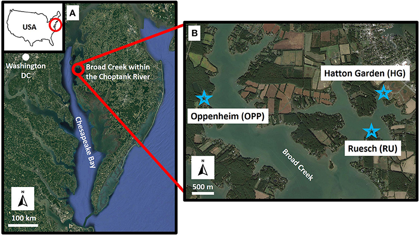
Figure 1. (A) Study area framing within the Chesapeake Bay (US). (B) The Broad Creek study site (Choptank River, MD). The stars mark the sites where deposition rates were measured in the field (Photo credits: Google Earth).

FIGURE 2

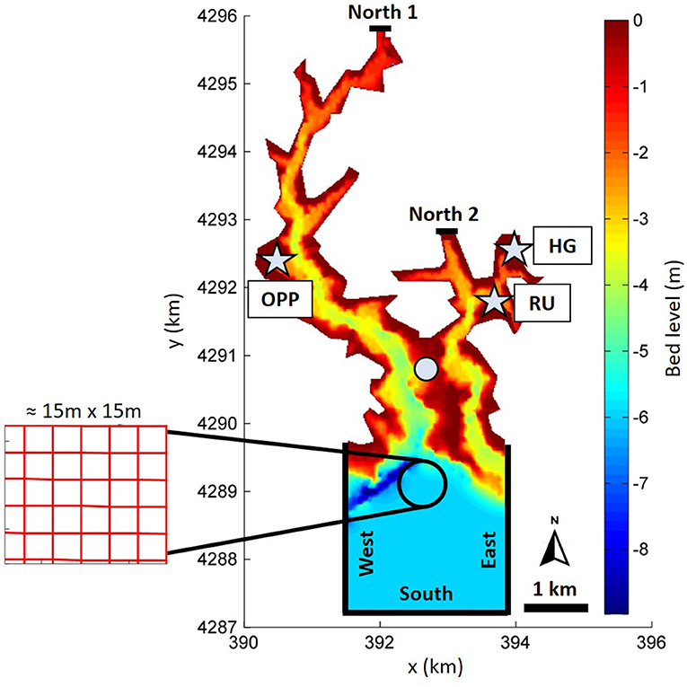
Figure 2. The Broad Creek numerical domain. Model bathymetry with the location of boundary conditions and deposition sites (stars). The white circle denotes the point at which water levels were validated.

The bottom stress was modeled with the formulation in the study by Chézy using a constant value equal to 55 m^1/2/s. The suspended-sediment eddy diffusivities were a function of the fluid eddy diffusivities and were calculated using a horizontal large eddy simulation and grain settling velocity. The horizontal eddy diffusivity coefficient was defined as a combination of the subgrid-scale horizontal eddy viscosity, computed from a horizontal large eddy simulation, and the background horizontal viscosity, which was set equal to 0.001 m²/s² in this study (Edmonds and Slingerland, 2010; Nardin et al., 2016). To satisfy the numerical stability criteria of Courant–Friedrichs–Lewy, we used a time step Δt = 6 s (Lesser et al., 2004). Each run simulates the morphological changes of 150 days under constant conditions during the simulation. To decrease the simulation time, we used a morphological scale factor equal to 10, a user device to multiply the deposition and erosion rates in each Δt. The morphological factor value was chosen to avoid numerical instability. We then multiplied the obtained deposition rate by 2.4 days to calculate the annual deposition.

Starting from the same numerical parameters used in the first modeling approach, we proceeded with the second idealized numerical model, where we varied wave height, wave period, and basin slope. A double nesting grid was used to propagate the wave motion well (Supplementary Figure 1). The outer and coarser wave grid was composed of 51 and 91 cells in the x and y directions, respectively, with a constant resolution of 100 m × 100 m. The flow domain (nested to the wave grid) was 3 km × 2 km, the computational grid was composed of 102 cells in the x-direction and 126 cells in the y-direction, and it was gradually refined from the eastern side (40 m × 40 m) to the western (10 m × 10 m; Figure 3). Sensitivity analyses showed that the resolution of the domain did not considerably impact wave propagation (Supplementary Figure 2). We simulated three different scenarios, which were (1) marsh only, (2) marsh and SAV, and (3) marsh, SAV, and rip-rap.

FIGURE 3

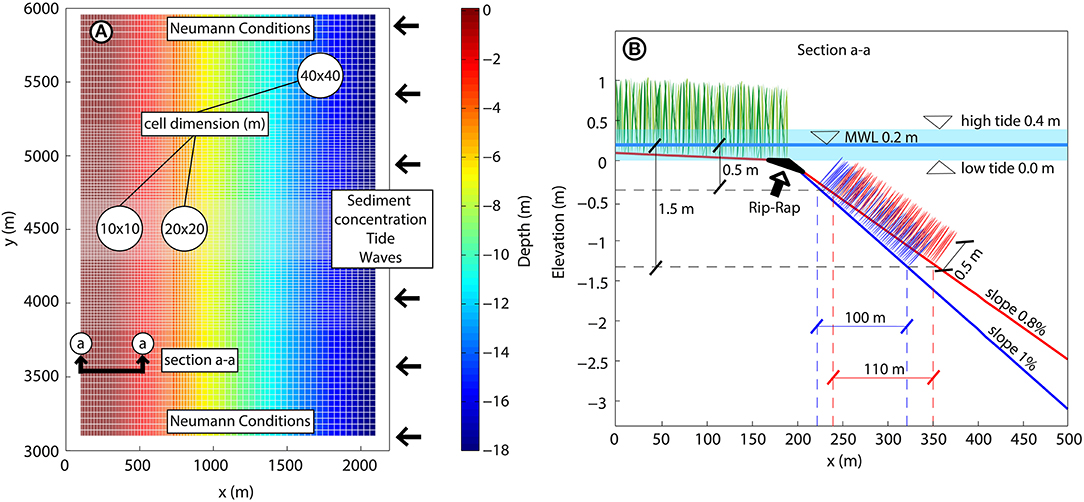
Figure 3. Flow domain configuration. (A) Planimetry of the model with cell dimensions and boundary conditions on the north/south side (Neumann condition) and east side (waves, tide, and suspended-sediment concentration). (B) Longitudinal profile (section a-a) of the domain with the two different slopes (blue line = 1% and red line = 0.8%) and related position of the submersed aquatic vegetation (SAV) bed [placed between 0.5 and 1.5 m below the mean water level (MWL), typical SAV depth in the Chesapeake Bay]. The top and the bottom limits of the area shaded in light blue represent high and low tides, respectively, and the dark blue line in the middle corresponds to the MWL.

To incorporate rip-rap into the simulations, we inserted a non-erodible bottom (thickness = 0) along the entire seaward boundary of the marsh to represent the rocks comprising the rip-rap. The initial condition set in the models was a fixed water level at 0.4 m with 5 m of an erodible bed level, composed of 50% sandy and 50% of muddy sediment with the same characteristics described above. The boundary conditions we imposed were the Neumann type for the northern and southern boundaries and a combination of water-level variation, incoming waves, and incoming suspended-sediment concentration for the eastern boundary. In the vertical direction, five non-homogeneous sigma layers were used, decreasing the layer thickness (%) of the local water depth for each layer going down to the bottom.

We varied the wave height (0.2, 0.3, 0.4, 0.5, 0.7, and 1 m), wave period (2, 3, 4, and 5 s), and basin slope (0.8 and 1%, as found by Koskelo et al., 2018 within the Choptank watershed and (Wiberg et al., 2019) at the Virginia Coastal Reserve), while the suspended-sediment concentration was fixed to 0.1 kg/m³. Wave parameters (H_s and T_p) were selected to simulate waves generated in the Chesapeake Bay (Lin et al., 2002) and were directed orthogonally to the shoreline. We imposed these values at the eastern boundary of the wave grid. Wave reflection was not accounted for in the wave model, so wave energy was dissipated at the coastline. To satisfy the numerical stability criteria of Courant–Friedrichs–Lewy we used a time step Δt = 3 s (Lesser et al., 2004). Each run simulated the morphological changes for 10 days under constant conditions during the simulation. To decrease the simulation time, we used a morphological scale factor equal to five. Aside from the Broad Creek model, the morphological factor value was chosen to avoid numerical instability.

The simulations were carried out by maintaining a constant wave height while everything else varied, for all simulated wave heights, then a constant wave period with everything else variable, and so on (Table 2). We completed 144 simulations in total.

TABLE 2

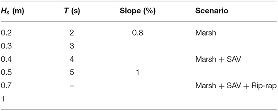
Table 2. Parameters for run combination.

Results

Our focus was on understanding the sediment exchange between the created marshes of living shorelines and adjacent SAV beds using the coupled Delft3D-SWAN model. In this section, we first compare the model results to field observations for validation, then present the hydrodynamic and morphodynamic results from the idealized model.

Model Validation

The estimation of the deposition rate made in the study by Bolton (2020) (performed along predefined transects) was carried out in the field from October 18, 2017 (HG and RU) to October 19, 2018 (OPP) for about 2 months. Then, annual deposition was extracted using lab techniques [see Bolton (2020) for further details]. Model validation was performed using the same timeframe as the sediment core samples. We ran two simulations for both years 2017 and 2018, from October 18 to November 3. The duration of the simulations was chosen in order to represent real conditions, but, at the same time, to have a reasonable computational time. The validation of the deposition rates was carried out along transects corresponding to 10 model cells, placed in correspondence with the measurement areas used in the study by Bolton (2020) (Figure 4). The obtained values were equal to the average obtained along the transects. The model predicted the deposition rates well in both years. Overall, deposition was underestimated for the three study sites but was still close to the real rate. Hatton Garden was more underestimated in 2017 but was closer to the real value in 2018, while OPP and RU were close in both years (Figure 5A).

FIGURE 4

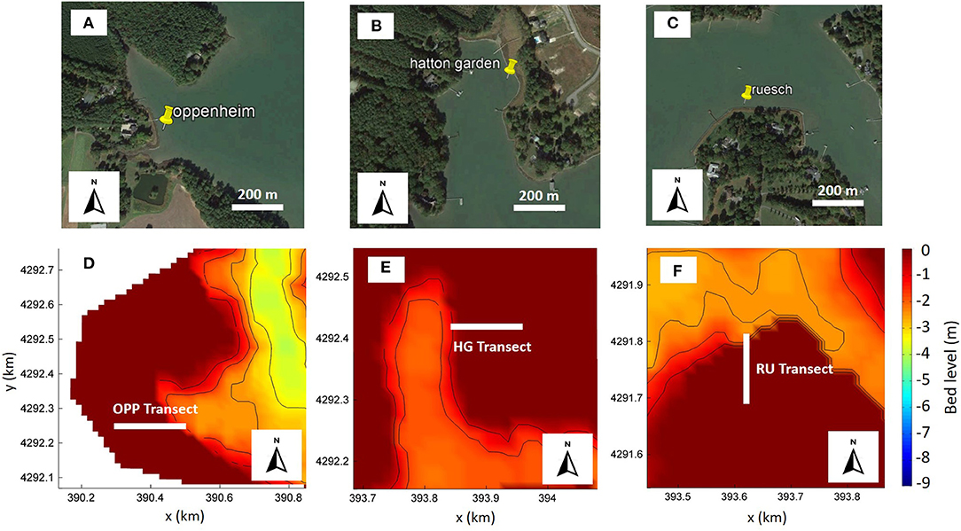
Figure 4. Study sites with the respective transects considered in the model. (A) Oppenheim site with (D) the corresponding transect used in the model to validate the deposition rate. (B) Hatton garden with (E) the corresponding transect used in the model to validate the deposition rate. (C) Ruesch with (F) the corresponding transect used in the model to validate the deposition rate (Photo credits: Google Earth).

FIGURE 5

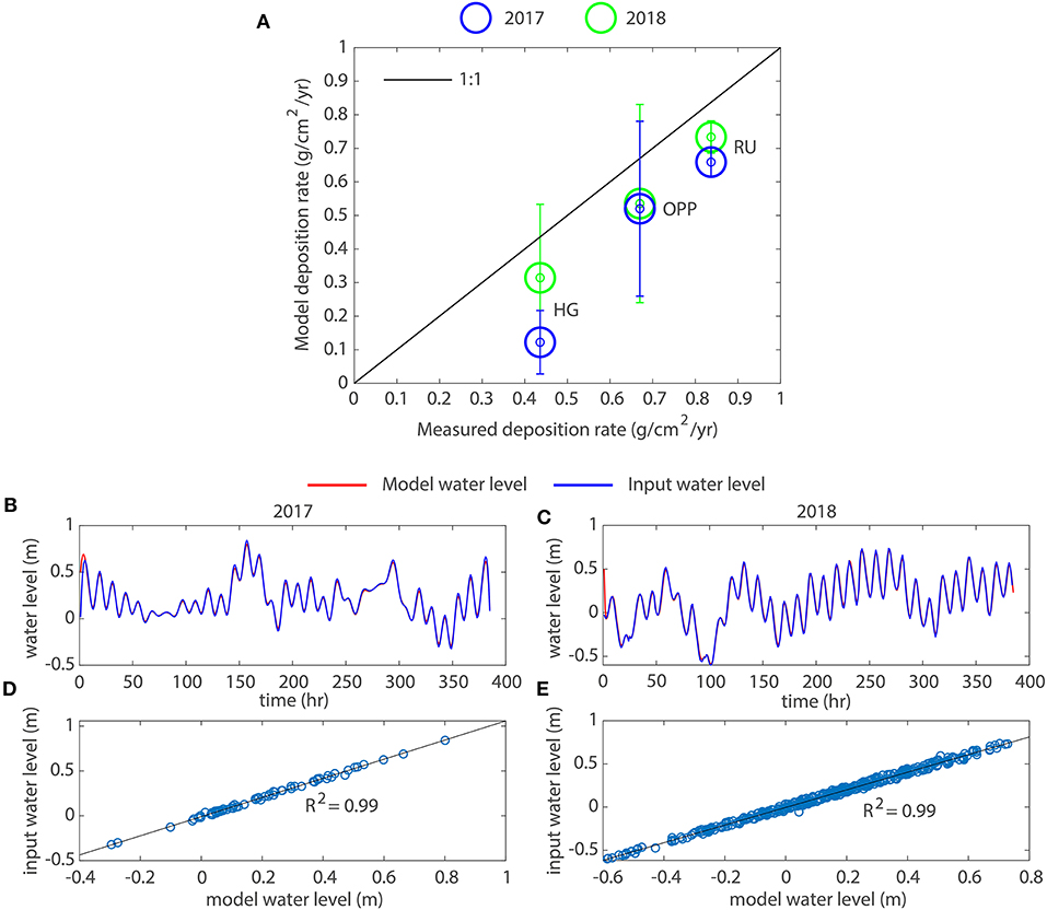
Figure 5. (A) Deposition rate validation obtained from the model. Error bars refer to above and below an SD. (B,D) Water level validation for the year 2017. (C,E) Water level validation for the year 2018.

The SD showed significant variability of the deposition rate along the OPP transect and more contained variation along the HG and RU transects.

The underestimation of the deposition rate was likely attributable to the lack of waves in the modeling. Waves within the Chesapeake Bay are of the order of 20–30 cm under normal conditions and reach 1 m in height in extreme events (Lin et al., 2002), allowing and amplifying solid transport.

The water level extracted from the CBOFS was well-predicted by the model for both simulated years, showing high correlation coefficients (Figures 5B–E).

Hydrodynamic Results

Model results showed an average wave reduction between 10 and 80% in incoming wave heights (Figure 6). Wave damping was similar for the three different configurations. The addiction of the SAV did not induce particular changes in wave height reduction compared with the marsh only scenario, while the presence of rip-rap resulted in a slight but greater wave height reduction for higher wave heights (Figure 6A). Wave damping was positively correlated with wave height following a linear law (Figure 6A), while shorter waves were dampened more than longer ones, which suffered a slight increase in height due to the shoaling effect (Figure 6B). The slope of the seabed did not particularly affect wave reduction; in contrast, it was more important for shear stress. Higher slopes led to greater shear stress values (Supplementary Figure 3). The shear stress at the bottom was significantly reduced within the SAV bed, but then rapidly increases before being drastically dampened by the marsh on the shore (Figure 7A). The shear stress at the beginning of the marsh (x = 200), for the configuration with only marsh on the shore, did not differ much from the scenario that also included the SAV, while the addition of rip-rap resulted in a reduction of shear stress values (Figures 7B,C) compared with both previous cases. Within the SAV bed, the marsh-only scenario produced the highest shear stress values (there was no SAV bed in the marsh-only scenario and, thus, less resistance to the flow), which were significantly reduced in the scenario that also included SAV. The addition of rip-rap resulted in shear stress values very close to the case with marsh and SAV (Figures 7D,E) and, thus, were lower than the marsh-only scenario. Shear stress was positively correlated with slope, wave height, and period following a power law. Wave height, however, appeared to have a greater impact on shear stress than wave period, as evidenced by the higher values of the correlation coefficient R² (Figures 7D,E).

FIGURE 6

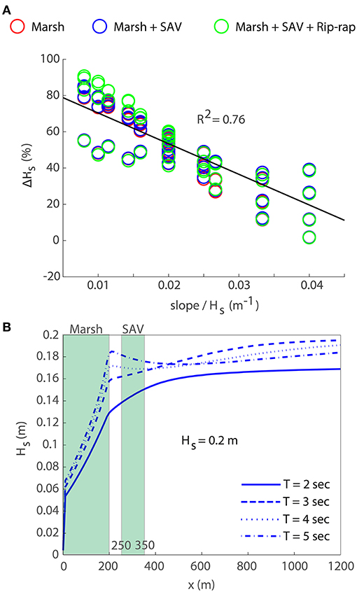
Figure 6. (A) The wave damping for all runs as a function of the variable slope/Hs. (B) Example of wave damping for the configuration with marsh and SAV, slope = 0.8%.

FIGURE 7

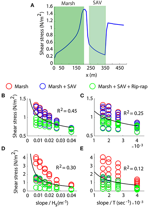
Figure 7. (A) Example of shear stress along the longitudinal direction for the simulation with both vegetation communities but no rip-rap, H_s = 0.3m, T = 4 s, and slope = 0.8%. (B) Shear stress value at the beginning of the marsh (x = 200 m) for the slope = 0.8%, as functions of the variable slope/Hs and (C) slope/T. (D) Average shear stress value within the SAV bed for the slope = 0.8%, as functions of the variable slope/Hs and (E) slope/T.

Morphodynamic Results

The sedimentation within the marsh was proportional to wave height and period for all simulated scenarios. The sedimentation for the marsh-only configuration was almost the same as the case with marsh and SAV, which did not significantly impact the deposition in the marsh. The marsh, SAV, and rip-rap scenario resulted in a slightly higher deposition for larger waves and slightly lower deposition for smaller waves (Figures 8A–C).

FIGURE 8

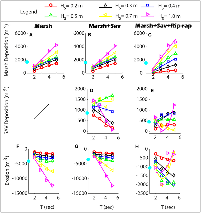
Figure 8. Summary of marsh and SAV deposition, and erosion for the different simulated scenarios with slope = 0.8%. (A,F) refer to the case with the only marsh. (B,D,G) refers to the case with marsh and SAV. (C,E,H) refer to the case with both vegetation communities and the rip-rap. The light blue dot on the y-axis denotes the mean value.

The deposition within the SAV bed varied according to the considered scenario. The case with the marsh only did not include any submerged vegetation and resulted in erosion within the location of the SAV bed, without any accumulation. The configuration with marsh and SAV, on the other hand, allowed the sedimentation inside the SAV bed to be proportional to wave height and inversely proportional to the period up to wave heights equal to 0.4 m. For wave heights equal to 0.5 m, deposition was also proportional to the period. Higher waves showed a decrease in deposition associated with greater shear stress values, which caused the erosion of the space in between marsh and SAV that we defined as “scarp,” also including part of the SAV bed (Figure 8D). The scenario with marsh, SAV, and rip-rap showed less deposition in the SAV compared with the case with marsh and SAV, but it was greater than the marsh-only scenario. The accumulation within the SAV bed was proportional to wave height and period up to wave heights equal to 0.4 m. Higher wave heights and periods led to higher shear stress values and wave reflection due to rip-rap, which resulted in less deposition. However, wave heights equal to 1 m were able to transport the greatest amount of sediment when accompanied by longer periods, thanks to the sediment resuspension caused by the high shear stress values (Figure 8E).

We calculated the erosion as the negative difference between the initial and final bed level (this included the marsh, the SAV, and the “scarp”). The erosion was proportional to both period and wave height for scenarios with marsh only and both marsh and SAV (Figures 8F,G). The scenario that also included the rip-rap reduced the erosion by an order of magnitude when compared with the other two cases. Erosion was proportional to wave height and period up to wave heights equal to 0.5 m. Higher wave heights (0.7 and 1 m) were capable of decreasing erosion since more deposition was associated with these conditions. Extreme events were capable of resuspension and transport the highest amount of sediments thanks to their high shear stress values, which allowed the replenishment of the shoreline with sediment, subsequently reducing erosion down to values close to zero (Figure 8H).

On average, marsh deposition was similar for all simulated scenarios, wherein there was slightly higher deposition for the marshy-only scenario compared with the other two. The deposition in the SAV was reduced by the presence of rip-rap compared with the case with marsh and SAV. Erosion was slightly reduced in the marsh + SAV scenario compared with the marsh only, while it was drastically reduced in the case that also included rip-rap. The structure protected the marsh edge from being eroded, resulting in less erosion than the two cases without rip-rap but increased wave reflection, further resulting in the greater erosion of the SAV bed (Figure 8).

The increase in basin slope resulted in less deposition within the marsh, greater deposition in the SAV, and higher erosion compared with the gentler slope (Supplementary Table 1).

We then estimated the percentage of deposition in the marsh, in the SAV, and erosion for each of the three examined configurations with respect to the sum of deposition (marsh + SAV) and the absolute value of erosion of each scenario (Figure 9). We distinguished erosion according to whether it was a marsh, SAV or scarp (we defined scarp as the space in between the marsh edge and the SAV bed). The marsh-only scenario resulted in 31% deposition and 69% erosion (Figure 9A). The 45% of the deposition in the marsh was caused by storms, while the erosion affected the marsh for 53% and the scarp for the remaining 47% (Figure 9D). The marsh and SAV scenario reduced erosion and increased deposition compared with the marsh only case. It resulted in 28% deposition in the marsh, 15% deposition in the SAV, and 57% of the erosion (Figure 9B). The 44% of the deposition in the marsh was caused by storms, extreme events impacted the deposition in the SAV for only 34%, and erosion was divided into 60% marsh, 30% scarp, and 10% SAV (Figure 9E). The marsh, SAV, and rip-rap scenario reduced erosion and increased deposition compared with the other two cases. It resulted in 50% deposition in the marsh, 16% deposition in the SAV, and 34% of the erosion (Figure 9C). The 60% of the deposition in the marsh was caused by storms, the extreme events impacted the deposition in the SAV by 27%, and erosion was divided into 70% scarp and 30% SAV (Figure 9F).

FIGURE 9

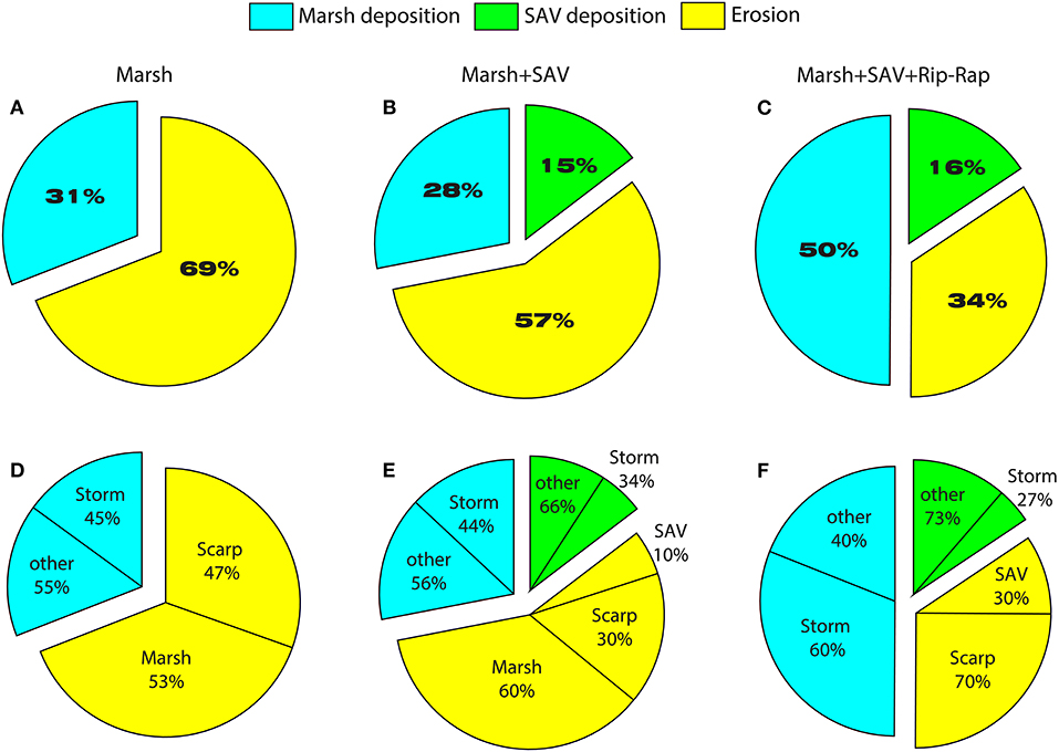
Figure 9. Deposition and erosion rates for each scenario. (A,D) refers to the case with the only marsh; (B,E) refers to the case with marsh and SAV; (C,F) refers to the case with marsh, SAV, and rip-rap. (A) Percentage of erosion and deposition in the marsh and (D) subdivision of the deposition depending on whether it was caused by storm or other and erosion depending on whether it was marsh or scarp. (B) Percentage of deposition in the marsh, in the SAV, erosion and (E) subdivision of the deposition according to whether it was caused by storm or other and erosion depending on whether it was a marsh, SAV or scarp. (C) Percentage of deposition in the marsh, in the SAV, erosion and (F) subdivision of the deposition according to whether it was caused by storm or other and erosion depending on whether it was a marsh, SAV or scarp.

We calculated, starting from erosion and deposition results, the sediment balance that occurred between marsh and SAV among all simulated scenarios. The sediment balance was defined as deposition into marsh + deposition into SAV – erosion, and it was calculated using the control domain shown in Figure 10. The sediment budget quantification is shown in Figure 11 for the different wave heights. Results were averaged over the period.

FIGURE 10

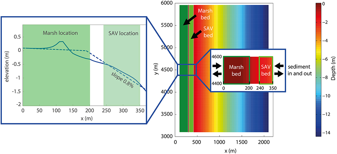
Figure 10. Domain for sediment budget calculation for the scenario with basin slope = 0.8%.

FIGURE 11

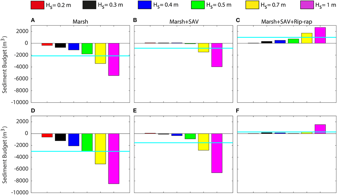
Figure 11. Sediment balance between the various simulated scenarios averaged over the wave period. (A–C) show the sediment budget for the scenario with slope = 0.8%, while (D–F) refer to slope = 1%. Left column (A,D) refers to the case with the only marsh; mid column (B,E) to the case with marsh and SAV; right column (C,F) to the case with both vegetations and rip-rap. The light blue line denotes the mean value.

The sediment balance was negative for the configuration that only included the marsh on the shore, indicating a net loss of sediment that was higher for the increased slope (Figures 11A,D). The sediment balance with both vegetation communities drastically reduced sediment loss for low-energy and slope scenarios but still had a higher amount of sediment loss for higher energy and slope scenarios. The sediment budget was positive (close to zero) for almost all of the simulated cases with a low slope, except for the extreme wave heights, 0.7 and 1 m. The balance was negative at the higher slope even for waves equal to 0.3, 0.4, and 0.5 m (Figures 11B,E). The configuration with marsh, SAV, and rip-rap resulted in a higher sediment retainment for all wave conditions. The sediment budget was slightly positive under the action of ordinary external forcing. For higher wave heights, which caused the greatest loss of sediments in the other two configurations, the sediment balance was strongly positive for gentle slopes, while it resulted in less accentuation for greater slopes (Figures 11C,F).

The effect of increasing the wave period was an increase in the loss of sediments (scenario with marsh only and both marsh and SAV) while allowing greater gains in the scenario that also included rip-rap. Extreme events were associated with larger wave heights, but also with larger periods (Supplementary Figure 4).

A meaningful summary of the effect of the three different configurations on sediment balance is shown in Table 3, where the budget values were averaged over the different wave heights and periods. The marsh + SAV configuration greatly reduced sediment loss compared with the marsh only scenario, and the aspect was made even more evident when rip-rap was also included.

TABLE 3

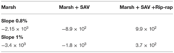
Table 3. Average sediment budget for the three different scenarios.

Discussion

Comparison With Previous Studies

Our numerical experiment, which couples Delft3D–SWAN, revealed the pivotal role of sediment interchange between the created saltmarsh of a living shoreline and its adjacent SAV. Simulation results demonstrated the efficacy of the vegetated shoreline in absorbing wave motion, thereby reducing incoming wave height by up to 80% according to a study by Manis et al. (2015), which found a wave energy reduction by Crassostrea virginica (eastern oyster) and Spartina alterniflora up to 67% in a wave tank experiment. Longer waves undergo an increase in height due to the shoaling effect, and according to a study by Battjes et al. (2004), they are nearly fully reflected at the shoreline, while higher-frequency components are subject to significant dissipation in narrow inshore zones including swash zones. Our model neglected wave reflection, so wave energy was all dissipated at the coast, which may result in greater erosion caused by longer waves. The model lacked the sensitivity to capture the SAV effect on wave height attenuation, which was mainly absorbed by the marsh, as well as by the friction at the bottom and wave breaking. However, previous studies have shown that submerged vegetation can attenuate wave height when vegetation height is comparable to water depth (Ward et al., 1984; Fonseca and Cahalan, 1992) and when wave orbital velocities and the seagrass canopy interact with each other (Chen et al., 2007). However, a study by Chen et al. (2007) highlighted that, to adequately assess the effect of SAV in coastal protection, its spatial and seasonal variability should be considered, together with the random variability of extreme events that mostly shape the coast and the spectral or directional distributions of wave energy. Our model kept the same wave direction orthogonal to the coastline for all simulations and the same vegetation density and height; thus, our results are limited to our study cases. Nevertheless, our model provided insight into the fundamental physical forces and principles underlying sediment transport and fate.

The higher shear stress values within the two vegetations were associated with longer periods, greater wave heights and basin slope, as found by Vona et al. (2020) regarding marshes and breakwaters interaction.

The modeling results showed the key role of waves in sedimentation and erosion. Extreme waves, with greater heights and periods, are capable of transporting the greatest amount of sediment within the marsh, but also have the greatest erosive power at the same time (Figure 8). Extreme events are also harmful to the SAV. The deposition was allowed more as the wave height increases, but storm conditions (wave height equal 0.7 and 1 m) erode the scarp mostly involving part of the SAV bed. However, the presence of rip-rap allowed deposition in the marsh as it greatly reduced erosion in case of extreme events, allowing the vegetation to obtain sediment supplies without suffering any losses. On the other hand, the artificial structure resulted in less deposition in the marsh in the case of normal external forcing. Studies in the literature have shown a similar behavior in waves when allowing sedimentation into the marsh (Castagno et al., 2018; Duvall et al., 2019; Nardin et al., 2020; Vona et al., 2020), also underlining the important role of other factors such as the alongshore current and the tide role in sediment retention within shallow coastal bays. On average, rip-rap resulted in a marked decrease in erosion. The marsh edge was protected by the structure and did not suffer any loss, but the rip-rap reflected incoming waves more, causing more erosion in the scarp and the SAV bed, which resulted in less deposition (Supplementary Table 1). Our model did not take into account the permeability of the break walls constituting rip-rap, since the structure was implemented in the model as an integral part of the bathymetry with a non-erodible bottom. The dissipative effects of the structure on transmitted waves were calculated using the wave transformation implemented in SWAN (wave–wave interactions, wave refraction, and wave dissipation by bottom friction and wave breaking), which did not take the effect of porosity into account. However, a study by Safak et al. (2020) investigated the effect of wave transmission through living shoreline break walls, finding that well-engineered semi-porous living shorelines act as buffers against human-mediated boat traffic and waves. They further underlined the benevolent aspects of coupling between natural and artificial solutions when studied correctly.

Our results highlighted the crucial role of SAV in coastal protection, as it reduces sediment export from the bay and allows sediment retention. This is in agreement with Donatelli et al. (2018), who highlighted the benevolent ability of seagrasses to the increase sediment storage capacity within shallow coastal bays. On the other hand, a decrease in seagrasses reduced the ability of the system to retain sediments, as our model shows when only the marsh occupies the shoreline, always determining a negative sedimentary balance. Donatelli et al. (2018) also pointed out that the presence of seagrasses reduces the suspended sediment concentration available for the marsh, with this aspect being slightly captured by our model as the deposition in the marsh was slightly higher in the absence of the SAV bed (Supplementary Table 1). However, a study by Chen et al. (2007) pointed out that, in order to fully understand the sediment retention mechanisms by the SAV, different sediment concentration inputs and transport within the bed due to currents should be taken into account. Our model maintained a constant inlet concentration of 0.1 kg/m³. A higher concentration would lead to more sedimentation in the marsh, as evidenced in the study by Vona et al. (2020), while deposition in the SAV would require further studies.

The presence of a non-erodible structure such as rip-rap slightly affected the sediment budget in the case of normal external forcing while helping stabilize the shoreline under extreme events. In storm conditions, solids transport in coastal wetlands was magnified, which implies the presence of rip-rap can be crucial in avoiding greater damage while allowing extreme events to replenish marshes and vegetated shorelines with sediments, as found in the studies by Castagno et al. (2018) and Vona et al. (2020).

The modeling results showed that hybrid infrastructures harnessed the benefits of both natural and built solutions to improve shoreline resilience. Moreover, by including vegetated features, hybrid systems are not likely to lose their effectiveness over time due to SLR, as in the case of submerged breakwaters for instance. This is because they can adapt themselves to SLR as long as they receive the right sediment replenishment, as shown in the study by Sutton-Grier et al. (2015).

Another important aspect to consider to improve the living shoreline configuration and make it more natural, while maintaining its efficiency, is the possibility of replacing the break walls constituting the rip-raps with oyster reefs. The advantage of integrating in-water infrastructure with oysters is that these reefs have the ability to grow with SLR (Rodriguez et al., 2014; Ridge et al., 2017), providing greater guarantees in terms of coastal protection even after the gray structure may become ineffective.

Interactions between vegetation species will play a key role in determining coastal wetlands responding to SLR and extreme events, and it will be crucial to keep understanding and monitoring feedback between different plant communities to better safeguard our coastal environments.

However, the evolution of vertical and horizontal marshes over time is a topic that still requires future research. Vertically, marshes need to accumulate sediments to contrast SLR, while horizontally, they need landward expansion to compensate for erosion (Fagherazzi et al., 2020). The dynamics of marsh evolution will require future studies to provide us with tools to safeguard our coasts.

Model Limitations

Delft3D-SWAN is a three dimensional, depth-averaged software for hydrodynamic computation. Hydraulic roughness due to vegetation is modeled, for rigid vegetation, by Baptist equations (Baptist, 2005), while for flexible vegetation, Delft3D assumes a greater degree of roughness (Lera et al., 2019).

However, models did provide useful insights on sediment transport and fate. In fact, we were able to model the mass balance of sediment distribution by coupling the hydrodynamic module with the vegetation model in the study of Baptist, with the possibility of adding different sediment characteristics (Nardin et al., 2020; Vona et al., 2020).

Baptist's equation has been widely tested with field and laboratory experiments, such as in the Allier River (France), the Volga River (Russia), and the Rhine River (Netherlands), with natural and artificial vegetation, coming to the conclusion that the model predicted sedimentation differences caused by vegetation well. Many experiments, compared with the results in the study of Baptist, gave back comparable outcomes. Recently, the study of Crosato and Saleh (2011) provided another validation of the Baptist equation with field observations applied to the Allier River in France. Moreover, the study of Baptist et al. (2007) used the results of the depth-averaged kappa–epsilon turbulence model, which accounts for vegetation in a genetic programming framework, to obtain an expression for roughness in the presence of vegetation, using a variety of input parameters to find the dimensionally consistent, symbolic equation.

Guidelines for “Living Shoreline” Implementation and Success

Coastal communities face ever harder challenges due to the rise of extreme events and SLR. Coastal stabilization solutions do not only require the implementation of engineering techniques, such as breakwaters or bulkheads, since new stabilization options, such as the living shoreline, can reduce erosion and man-made structures while providing ecosystem services such as food production, nutrient removal, and water quality improvement (NOAA, 2015).

However, the success of vegetation planting for coastal protection is not always guaranteed, as it depends on various factors that can affect plant resilience. One of the most important factors is wave climate. Wave climate is influenced by factors such as fetch, wind speed and duration, water depth, basin slope, and the orientation of the site. When a shoreline is facing the storm wind direction, it is more likely to be damaged, while a shallow water environment with a gentle slope is more capable of reducing wave energy and protecting plant species. Other important factors for the living shoreline survival are constant sediment supply, given by periodic tidal flooding, nutrient supply and salinity, and many others that can be found in the study of Broome et al. (1992). Given the dependence of the planting success on the geographical site, the study results highlighted how the ideal conditions are found for living shoreline installation, as the simultaneous presence of marsh and SAV greatly helps to reduce the sediment loss outgoing coastal wetlands. This improves the resilience and ensures the better stabilization of the shore, while rip-rap considerably helps with storm conditions (Figure 12). Our work can give good indications on the implementation of coastal recovery and maintenance plans in shallow coastal bays, given wave climate and bathymetric conditions, through natural solutions that look at both the protection and the ecology of coastal environments.

FIGURE 12

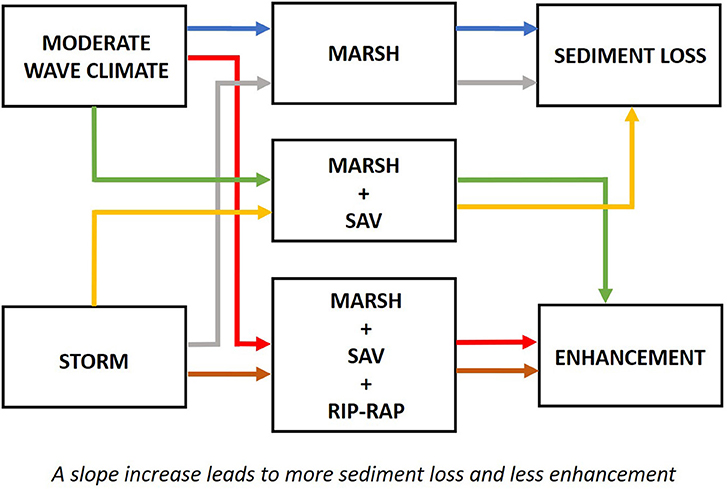
Figure 12. Feedback between wave climates and living shoreline configuration in the sediment budget.

Conclusion

Understanding sediment transport dynamics is crucial for coastal protection. Our study provided references for decision makers working in coastal wetland restoration. In this study, we investigated the sediment interchange between saltmarshes and SAV to better quantify the synergy between the two plant communities. The SAV certainly helped enhance shoreline resilience, reducing sediment loss by retaining the sediments outgoing the marsh and allowing deposition. The presence of non-erodible structures such as rip-rap, which is often an integral part of the living shoreline, protects against extreme events and allows sediment replenishment inside the marsh, especially under storm conditions. The delicate balance between the supply and loss of sediments is crucial in coastal wetland restoration. Artificial structures make it possible to avoid greater damage in extreme events, which also has a significant economic impact. Living shorelines certainly offer a valid and green solution to coastal protection, which, if coupled with man-made or natural structures, such as oyster reefs rather than rip-rap, can strengthen the resilience and the vitality of the coast.

Data Availability Statement

The original contributions presented in the study are included in the article/Supplementary Material, further inquiries can be directed to the corresponding author/s.

Author Contributions

IV took part in most works of this research, including writing the manuscript, designing the model experiments, running the model, and analyzing the results. WN and CP revised the article and gave advice on the manuscript structure. All authors contributed to the article and approved the submitted version.

Conflict of Interest

The authors declare that the research was conducted in the absence of any commercial or financial relationships that could be construed as a potential conflict of interest.

The handling Editor declared a past co-authorship with one of the authors WN.

Publisher's Note

All claims expressed in this article are solely those of the authors and do not necessarily represent those of their affiliated organizations, or those of the publisher, the editors and the reviewers. Any product that may be evaluated in this article, or claim that may be made by its manufacturer, is not guaranteed or endorsed by the publisher.

Acknowledgments

This is contribution 6044 of the University of Maryland Center for Environmental Science - Horn Point Laboratory.

Supplementary Material

The Supplementary Material for this article can be found online at: https://www.frontiersin.org/articles/10.3389/fmars.2021.727080/full#supplementary-material

References

Arboleda, A. M., Crosato, A., and Middelkoop, H. (2010). Reconstructing the early 19th-century Waal River by means of a 2D physics-based numerical model. Hydrol. Process. 24, 3661–3675. doi: 10.1002/hyp.7804

CrossRef Full Text | Google Scholar

Baptist, M. J. (2005). Modelling Floodplain Biogeomorphology Baptist 2005. Delft: Delft University Press.

Google Scholar

Baptist, M. J., Babovic, V., Rodríguez Uthurburu, J., Keijzer, M., Uittenbogaard, R. E., Mynett, A., et al. (2007). On inducing equations for vegetation resistance. J. Hydraul. Res. 45, 435–450. doi: 10.1080/00221686.2007.9521778

CrossRef Full Text | Google Scholar

Barbier, E. B., Hacker, S. D., Kennedy, C., Koch, E. W., Stier, A. C., and Silliman, B. R. (2011). The value of estuarine and coastal ecosystem services. Ecol. Monogr. 81, 169–193. doi: 10.1890/10-1510.1

CrossRef Full Text | Google Scholar

Barko, J. W., Gunnison, D., and Carpenter, S. R. (1991). Sediment interactions with submersed macrophyte growth and community dynamics. Aquat. Bot. 41, 41–65. doi: 10.1016/0304-3770(91)90038-7

CrossRef Full Text | Google Scholar

Battjes, J. A., Bakkenes, H. J., Janssen, T. T., and van Dongeren, A. R. (2004). Shoaling of subharmonic gravity waves. J. Geophys. Res. 109:C02009. doi: 10.1029/2003JC001863

CrossRef Full Text | Google Scholar

Battjes, J. A., and Janssen, J. P. F. M. (1978). “Energy loss and set-up due to breaking of random waves,” in Coastal Engineering, 569–587.

Google Scholar

Berlamont, J., Ockenden, M., Toorman, E., and Winterwerp, J. (1993). The characterisation of cohesive sediment properties. Coast. Eng. 21, 105–128. doi: 10.1016/0378-3839(93)90047-C

CrossRef Full Text | Google Scholar

Bilkovic, D. M., and Mitchell, M. M. (2013). Ecological tradeoffs of stabilized salt marshes as a shoreline protection strategy: effects of artificial structures on macrobenthic assemblages. Ecol. Eng. 61, 169–481. doi: 10.1016/j.ecoleng.2013.10.011

CrossRef Full Text | Google Scholar

Bolton, M. (2020). Evaluating Feedbacks between Vegetation and Sediment Dynamics in Submersed Aquatic Vegetation (SAV) Beds and Created Marshes of Living Shorelines in Chesapeake Bay [MS Thesis]. University of Maryland, College Park. MD.

Google Scholar

Boorman, L. A. (1999). Salt marshes-present functioning and future change. Mangroves Salt Marshes 3, 227–241.

Google Scholar

Bricker-Urso, S., Nixon, S. W., Cochran, J. K., Hirschberg, D. J., and Hunt, C. (1989). Accretion rates and sediment accumulation in Rhode Island salt marshes. Estuaries 12, 300–317. doi: 10.2307/1351908

CrossRef Full Text | Google Scholar

Broome, S. W., Rogers, S. M. Jr., and Seneca, E. D. (1992). Shoreline Erosion Control Using Marsh Vegetation and Low-Cost Structures. UNC-SG-92-12. North Carolina Sea Grant Program Publication.

Google Scholar

Burke, D. G., Koch, E. W., and Stevenson, J. C. (2005). Assessment of Hybrid Type Shore Erosion Control Projects in Maryland's. Chesapeake Bay: Phases I and II. Maryland Department of Natural Resources.

Google Scholar

Carter, V., Rybicki, N. B., Landwehr, J. M., and Turtora, M. (1994). Role of weather and water quality in population dynamics of submersed macrophytes in the tidal Potomac River. Estuaries 17, 417–426. doi: 10.2307/1352674

CrossRef Full Text | Google Scholar

Castagno, K. A., Jiménez-Robles, A. M., Donnelly, J. P., Wiberg, P. L., Fenster, M. S., and Fagherazzi, S. (2018). Intense storms increase the stability of tidal bays. Geophys. Res. Lett. 45, 5491–5500. doi: 10.1029/2018GL078208

CrossRef Full Text | Google Scholar

Catling, P. M., Spicer, K. W., Biernachi, M., and Lovett Doust, J. (1994). The biology of Canadian weeds: 103. Can. J. Plant Sci. 74, 883–897. doi: 10.4141/cjps94-160

CrossRef Full Text | Google Scholar

Chen, S. N., Sanford, L. P., Koch, E. W., Shi, F., and North, E. W. (2007). A nearshore model to investigate the effects of seagrass bed geometry on wave attenuation and suspended sediment transport. Estuaries Coasts 30, 296–310. doi: 10.1007/BF02700172

CrossRef Full Text | Google Scholar

Cotton, J. A., Wharton, G., Bass, J. A. B., Heppell, C. M., and Wotton, R. S. (2006). The effects of seasonal changes to in-stream vegetation cover on patterns of flow and accumulation of sediment. Geomorphology 77, 320–324. doi: 10.1016/j.geomorph.2006.01.010

CrossRef Full Text | Google Scholar

Crosato, A., and Saleh, M. S. (2011). Numerical study on the effects of floodplain vegetation on river planform style. Earth Surf. Process. Landforms 36, 711–720 doi: 10.1002/esp.2088

CrossRef Full Text | Google Scholar

Currin, C. A., Chappell, W. S., and Deaton, A. (2010). “Developing alternative shoreline armoring strategies: the living shoreline approach in North Carolina,” in Puget Sound Shorelines and the Impacts of Armoring-Proceedings of a State of the Science Workshop (U.S. Geological Survey), 92–102.

Google Scholar

Davis, J. L., Currin, C. A., O'Brien, C., Raffenburg, C., and Davis, A. (2015). Living shorelines: coastal resilience with a blue carbon benefit. PLoS One 10:e0142595. doi: 10.1371/journal.pone.0142595

PubMed Abstract | CrossRef Full Text | Google Scholar

Donatelli, C., Ganju, N. K., Fagherazzi, S., and Leonardi, N. (2018). Seagrass impact on sediment exchange between tidal flats and salt marsh, and the sediment budget of shallow bays. Geophys. Res. Lett. 45, 4933–4943. doi: 10.1029/2018GL078056

CrossRef Full Text | Google Scholar

Duvall, M. S., Wiberg, P. L., and Kirwan, M. L. (2019). Controls on sediment suspension, flux, and marsh deposition near a bay-marsh boundary. Estuaries Coasts 42, 403–424. doi: 10.1007/s12237-018-0478-4

CrossRef Full Text | Google Scholar

Edmonds, D. A., and Slingerland, R. L. (2010). Significant effect of sediment cohesion on delta morphology. Nat. Geosci. 3, 105–109. doi: 10.1038/ngeo730

CrossRef Full Text | Google Scholar

Ensign, S. H., Noe, G. B., and Hupp, C. R. (2014). Linking channel hydrology with riparian wetland accretion in tidal rivers. J. Geophys. Res. Earth Surf. 119, 28–44. doi: 10.1002/2013JF002737

CrossRef Full Text | Google Scholar

Fagherazzi, S., Mariotti, G., Leonardi, N., Canestrelli, A., Nardin, W., and Kearney, W. S. (2020). Salt marsh dynamics in a period of accelerated sea level rise. J. Geophys. Res. Earth Surf. 125:e2019JF005200. doi: 10.1029/2019JF005200

CrossRef Full Text | Google Scholar

Fonseca, M. S., and Cahalan, J. A. (1992). A preliminary evaluation of wave attenuation by four species of seagrass. Estuar. Coast. Shelf Sci. 35, 565–576. doi: 10.1016/S0272-7714(05)80039-3

CrossRef Full Text | Google Scholar

Ganju, N. K., Defne, Z., Elsey-Quirk, T., and Moriarty, J. M. (2019). Role of tidal wetland stability in lateral fluxes of particulate organic matter and carbon. J. Geophys. Res. 124, 1265–1277. doi: 10.1029/2018JG004920

CrossRef Full Text | Google Scholar

Ganju, N. K., Nidzieko, N. J., and Kirwan, M. L. (2013). Inferring tidal wetland stability from channel sediment fluxes: Observations and a conceptual model. J. Geophys. Res. Earth Surf. 118, 2045–2058. doi: 10.1002/jgrf.20143

CrossRef Full Text | Google Scholar

Gittman, R. K., Peterson, C. H., Currin, C. A., Fodrie, F. J., Piehler, M. F., and Bruno, J. F. (2016a). Living shorelines can enhance the nursery role of threatened estuarine habitats. Ecol. Appl. 26, 249–263 doi: 10.1890/14-0716

PubMed Abstract | CrossRef Full Text | Google Scholar

Gittman, R. K., Scyphers, S. B., Smith, C. S., Neylan, I. P., and Grabowski, J. H. (2016b). Ecological consequences of shoreline hardening: a meta-analysis. Bioscience 66, 763–773. doi: 10.1093/biosci/biw091

PubMed Abstract | CrossRef Full Text | Google Scholar

Grabowski, J. H., Brumbaugh, R. D., Conrad, R. F., Keeler, A. G., Opaluch, J. J., Peterson, C. H., et al. (2012). Economic valuation of ecosystem services provided by oyster reefs. Bioscience 62, 900–909. doi: 10.1525/bio.2012.62.10.10

CrossRef Full Text | Google Scholar

Hasselmann, K. F., Barnett, T. P., Bouws, E., Carlson, H., Cartwright, D. E., Eake, K., et al. (1973). Measurements of Wind-Wave Growth and Swell Decay During the Joint North Sea Wave Project (JONSWAP). Ergaenzungsheft zur Deutschen Hydrographischen Zeitschrift, Reihe A.

Google Scholar

Heck, K., Able, K. W., Roman, C. T., and Fahay, M. P. (1995). Composition, abundance, biomass, and production of macrofauna in a New England estuary: comparisons among eelgrass meadows and other nursery habitats. Estuaries 8, 379–389. doi: 10.2307/1352320

CrossRef Full Text | Google Scholar

Koskelo, A. I., Fisher, T. R., Sutton, A. J., and Gustafson, A. B. (2018). Biogeochemical storm response in agricultural watersheds of the Choptank River Basin, Delmarva Peninsula, USA. Biogeochemistry 139, 215–239. doi: 10.1007/s10533-018-0464-8

CrossRef Full Text | Google Scholar

Lera, S., Nardin, W., Sanford, L., Palinkas, C., and Guercio, R. (2019). The impact of submersed aquatic vegetation on the development of river mouth bars. Earth Surf. Process. Landforms 44, 1494–1506. doi: 10.1002/esp.4585

CrossRef Full Text | Google Scholar

Lesser, G. R., Roelvink, J. A., van Kester, J. A. T. M., and Stelling, G. S. (2004). Development and validation of a three-dimensional morphological model. Coast. Engl. 51, 883–915. doi: 10.1016/j.coastaleng.2004.07.014

CrossRef Full Text | Google Scholar

Li, M., Zhang, F., Barnes, S., and Wang, X. (2020). Assessing storm surge impacts on coastal inundation due to climate change: case studies of Baltimore and Dorchester County in Maryland. Nat. Hazards 103, 2561–2588. doi: 10.1007/s11069-020-04096-4

CrossRef Full Text | Google Scholar

Lin, W., Sanford, L. P., and Suttles, S. E. (2002). Wave measurement and modeling in Chesapeake Bay. Cont. Shelf Res. 22, 2673–2686. doi: 10.1016/S0278-4343(02)00120-6

CrossRef Full Text | Google Scholar

Manis, J. E., Garvis, S. K., Jachec, S. M., and Walters, L. J. (2015). Wave attenuation experiments over living shorelines over time: a wave tank study to assess recreational boating pressures. J. Coast. Conserv. 19, 1–11. doi: 10.1007/s11852-014-0349-5

CrossRef Full Text | Google Scholar

Marra, J., Allen, T., Easterling, D., Fauver, S., Karl, T., Levinson, D., et al. (2007). An integrating architecture for coastal inundation and erosion program planning and product development. Mar. Technol. Soc. J. 41, 62–75. doi: 10.4031/002533207787442321

CrossRef Full Text | Google Scholar

Nardin, W., Edmonds, D. A., and Fagherazzi, S. (2016). Influence of vegetation on spatial patterns of sediment deposition in deltaic islands during flood. Adv. Water Resour. 93, 236–248. doi: 10.1016/j.advwatres.2016.01.001

CrossRef Full Text | Google Scholar

Nardin, W., Lera, S., and Nienhuis, J. (2020). Effect of offshore waves and vegetation on the sediment budget in the Virginia Coast Reserve (VA). Earth Surf. Process. Landforms 45, 3055–3068. doi: 10.1002/esp.4951

CrossRef Full Text | Google Scholar

NOAA, L. (2015). Guidance for Considering the Use of Living Shorelines.

Google Scholar

Noordhuis, R., Van Der Molen, D. T., and Van Der Berg, M. S. (2002). Response of herbivorous waterbirds to the return of Chara in Lake Veluwemeer, the Netherlands. Aquat. Bot. 72, 349–367. doi: 10.1016/S0304-3770(01)00210-8

CrossRef Full Text | Google Scholar

Palinkas, C. M., and Lorie, S. (2018). “Promoting living shorelines for shoreline protection: understanding potential impacts to and ecosystem trade-offs with adjacent submersed aquatic vegetation (SAV),” Presented at the AGU Fall Meeting 2018.

Google Scholar

Partheniades, E. (1965). Erosion and deposition of cohesive soils. J. Hydraul. Div. 91, 105–139. doi: 10.1061/JYCEAJ.0001165

CrossRef Full Text | Google Scholar

Ridge, J. T., Rodriguez, A. B., and Fodrie, F. J. (2017). Evidence of exceptional oyster-reef resilience to fluctuations in sea level. Ecol. Evol. 7, 10409–10420. doi: 10.1002/ece3.3473

PubMed Abstract | CrossRef Full Text | Google Scholar

Rodi, W., and Scheuerer, G. (1984). “Scrutinizing the k-epsilon-model under adverse pressure gradient conditions,” in 4th Symposium on Turbulent Shear Flows (Berlin; Heidelberg: Springer), 2–8.

Google Scholar

Rodriguez, A. B., Fodrie, F. J., Ridge, J. T., Lindquist, N. L., Theuerkauf, E. J., Coleman, S. E., et al. (2014). Oyster reefs can outpace sea-level rise. Nat. Clim. Chang. 4, 493–497. doi: 10.1038/nclimate2216

CrossRef Full Text | Google Scholar

Roelvink, J. A., and Van Banning, G. K. F. M. (1995). Design and development of DELFT3D and application to coastal morphodynamics. Oceanogr. Lit. Rev. 11:925.

Google Scholar

Safak, I., Angelini, C., Norby, P. L., Dix, N., Roddenberry, A., Herbert, D., et al. (2020). Wave transmission through living shoreline breakwalls. Cont. Shelf Res. 211:104268. doi: 10.1016/j.csr.2020.104268

CrossRef Full Text | Google Scholar

Schuerch, M., Spencer, T., Temmerman, S., Kirwan, M. L., Wolff, C., Lincke, D., et al. (2018). Future response of global coastal wetlands to sea-level rise. Nature 561, 231–234. doi: 10.1038/s41586-018-0476-5

PubMed Abstract | CrossRef Full Text | Google Scholar

Scyphers, S. B., Gouhier, T. C., Grabowski, J. H., Beck, M. W., Mareska, J., and Powers, S. P. (2015). Natural shorelines promote the stability of fish communities in an urbanized coastal system. PLoS One 10:e0118580. doi: 10.1371/journal.pone.0118580

PubMed Abstract | CrossRef Full Text | Google Scholar

Short, F. T., and Wyllie-Echeverria, S. (1996). Natural and human induced disturbance of seagrasses. Environ. Conserv. 23, 17–27. doi: 10.1017/S0376892900038212

CrossRef Full Text | Google Scholar

Sutton-Grier, A. E., Wowk, K., and Bamford, H. (2015). Future of our coasts: the potential for natural and hybrid infrastructure to enhance the resilience of our coastal communities, economies and ecosystems. Environ. Sci. Policy 51, 137–148. doi: 10.1016/j.envsci.2015.04.006

CrossRef Full Text | Google Scholar

Temmerman, S., Meire, P., Bouma, T. J., Herman, P. M., Ysebaert, T., and De Vriend, H. J. (2013). Ecosystem-based coastal defence in the face of global change. Nature 504, 79–83. doi: 10.1038/nature12859

PubMed Abstract | CrossRef Full Text | Google Scholar

Uittenbogaard, R. (2003). “Modelling turbulence in vegetated aquatic flows,” in International Workshop on RIParian FORest Vegetated Channels: Hydraulic, Morphological and Ecological Aspects (Trento).

Google Scholar

Van Rijn, L. C. (1993). Principles of Sediment Transport in Rivers, Estuaries and Coastal Seas, Vol. 1006. Amsterdam: Aqua Publications, 11–13.

Google Scholar

Vona, I., Gray, M. W., and Nardin, W. (2020). The impact of submerged breakwaters on sediment distribution along marsh boundaries. Water 12:1016. doi: 10.3390/w12041016

CrossRef Full Text | Google Scholar

Ward, L., Kemp, W., and Boyton, W. (1984). The influence of waves and seagrass communities on suspended particulates in an estuarine embayment. Mar. Geol. 59, 85–103. doi: 10.1016/0025-3227(84)90089-6

CrossRef Full Text | Google Scholar

Wharton, G., Cotton, J. A., Wotton, R. S., Bass, J. A. B., Heppell, C. M., Trimmer, M., et al. (2006). Macrophytes and suspension-feeding invertebrates modify flows and fine sediments in the From and Piddle catchments, Dorset (UK). J. Hydrol. 330, 171–184. doi: 10.1016/j.jhydrol.2006.04.034

CrossRef Full Text | Google Scholar

Wiberg, P. L., Taube, S. R., Ferguson, A. E., Kremer, M. R., and Reidenbach, M. A. (2019). Wave attenuation by oyster reefs in shallow coastal bays. Estuar. Coasts 42, 331–347.

Google Scholar

Zhu, Q., Wiberg, P. L., and Reidenbach, M. A. (2021). Quantifying seasonal seagrass effects on flow and sediment dynamics in a Back-Barrier Bay. J. Geophys. Res. Oceans 126:e2020JC016547. doi: 10.1029/2020JC016547

CrossRef Full Text | Google Scholar