 Daniella Hanf
 Amanda Jane Hodgson
 Halina Kobryn
 Lars Bejder
 Joshua Nathan Smith
- 1O2 Marine, Busselton, WA, Australia
- 2Cetacean Ecology, Behaviour and Evolution Lab, School of Biological Sciences, Flinders University, Adelaide, SA, Australia
- 3Centre for Sustainable Aquatic Ecosystems, Harry Butler Institute, Murdoch University, Murdoch, WA, Australia
- 4Environmental and Conservation Sciences, Murdoch University, Murdoch, WA, Australia
- 5Marine Mammal Research Program, Hawaii Institute of Marine Biology, University of Hawai‘i at Mānoa, Honolulu, HI, United States
- 6Section for Zoophysiology, Department of Bioscience, Aarhus University, Aarhus, Denmark
Understanding species’ distribution patterns and the environmental and ecological interactions that drive them is fundamental for biodiversity conservation. Data deficiency exists in areas that are difficult to access, or where resources are limited. We use a broad-scale, non-targeted dataset to describe dolphin distribution and habitat suitability in remote north Western Australia, where there is a paucity of data to adequately inform species management. From 1,169 opportunistic dolphin sightings obtained from 10 dugong aerial surveys conducted over a four-year period, there were 661 Indo-Pacific bottlenose dolphin (Tursiops aduncus), 191 Australian humpback dolphin (Sousa sahulensis), nine Australian snubfin dolphin (Orcaella heinsohni), 16 Stenella sp., one killer whale (Orcinus orca), one false killer whale (Pseudorca crassidens), and 290 unidentified dolphin species sightings. Maximum Entropy (MaxEnt) habitat suitability models identified shallow intertidal areas around mainland coast, islands and shoals as important areas for humpback dolphins. In contrast, bottlenose dolphins are more likely to occur further offshore and at greater depths, suggesting niche partitioning between these two sympatric species. Bottlenose dolphin response to sea surface temperature is markedly different between seasons (positive in May; negative in October) and probably influenced by the Leeuwin Current, a prominent oceanographic feature. Our findings support broad marine spatial planning, impact assessment and the design of future surveys, which would benefit from the collection of high-resolution digital images for species identification verification. A substantial proportion of data were removed due to uncertainties resulting from non-targeted observations and this is likely to have reduced model performance. We highlight the importance of considering climatic and seasonal fluctuations in interpreting distribution patterns and species interactions in assuming habitat suitability.
Introduction
Understanding the factors and mechanisms that underpin species’ distribution and ecology is critical for biodiversity conservation. Oceanic dolphins (Family: Delphinidae) are the most diverse family of marine mammals, consisting of 16 genera and 37 species (Jefferson and LeDuc, 2018). They have radiated and adapted, behaviourally and physiologically, to occupy a range of habitats and niches. As individuals’ fitness and population viability are directly linked to habitat quality, habitat degradation is recognised as a key cause of diminishing global biodiversity, including for marine mammals (Pimm et al., 1995; Novacek and Cleland, 2001; Ceballos et al., 2015; Avila et al., 2018; Nelms et al., 2021). Habitat loss or diminished habitat integrity can lead to a spatial or temporal shift in populations’ distribution. Species with high site fidelity or with small or restricted ranges, are particularly susceptible to displacement (Reed and Frankham, 2003; Banks et al., 2007; Tuomainen and Candolin, 2011; New et al., 2013; Forney et al., 2017) and although the consequence of displacement (e.g., by human disturbance or extreme environmental events) is difficult to predict, a shift to an area of suboptimal conditions may have negative population-level effects (Heithaus and Dill, 2002; New et al., 2013; Forney et al., 2017; Pirotta et al., 2018). For some populations, sub-lethal effects may have higher consequences and be longer lasting at the population level than direct harm to an individual may have (Forney et al., 2017). However, the mechanisms for such a consequence are not well understood. Identifying important habitats for species is a first step in being able to assess the likelihood and consequence severity of displacement. The shallow coastline of north Western Australia (WA) supports three coastal dolphin species: the Australian humpback (Sousa sahulensis) (“humpback”) dolphin; the Australian snubfin (Orcaella heinsohni) (“snubfin”) dolphin; and the Indo-Pacific bottlenose (Tursiops aduncus) (“bottlenose”) dolphin (Allen et al., 2012; Bejder et al., 2012). Respectively, they are internationally listed as “Vulnerable,” “Vulnerable,” and “Near Threatened” on the International Union for the Conservation of Nature’s Red List of Threatened Species (Parra et al., 2017a,b; IUCN, 2020). Humpback and snubfin dolphins are most at risk from sub-lethal effects of habitat disturbance due to their restricted distribution within northern Australia and small, discrete populations that spatially overlap with human activities (i.e., coastal development; petroleum exploration; commercial fishing; and recreational boating) (Parra et al., 2006a; Parra and Cagnazzi, 2016; Hanf et al., 2016; Bouchet et al., 2021). However, due to inadequate or unavailable information on their distribution, abundance and ecology for most of their range, they are ineligible to be considered as threatened species under Australia’s key biodiversity conservation legislation, the Environment and Biodiversity Protection Act 1999 (“EPBC Act”). Listed as a “Migratory” species by the Bonn Convention, they are recognised as EPBC Act Matters of National Environmental Significance (MNES), therefore requiring special consideration during the environmental impact assessment (EIA) process. Data deficiency in species’ distribution (i.e., exact range, important areas, habitat preferences, or ecological niche) is evident in remote WA, and this hinders the ability to conduct informed EIA (Allen et al., 2012; Bejder et al., 2012; Hanf et al., 2016; Waples and Raudino, 2018). The paradox is that funding is needed to obtain abundance and distribution data for these dolphins to be listed as threatened species, yet there would be a greater chance of funding being allocated for research if they were already designated as threatened.
Robust EIA, conservation programmes and management plans require species distribution data at broad spatial and temporal scales, as well as at the fine scale. Spatially, regional maps can depict species’ ranges, occurrences, biologically important areas, biodiversity hotspots and relative patterns in spatial density and abundance [e.g., Integrated Biodiversity Assessment Tool (IBAT), 2008; Tittensor et al., 2010; Australian Government, 2012a; Hammond et al., 2013; Corrigan et al., 2014; Atlas of Living Australia, 2019]. Information on temporal distribution patterns can be powerful in protecting species from human activity, through implementation of time-area closures (e.g., Tyne et al., 2012), avoidance of sensitive life history phases (Irvine et al., 2018) and the incorporation of seasonal and interannual climatic variation (Sprogis et al., 2017a).
Our study site is situated in the western Pilbara (WA) (Figure 1), within coastal waters of the lower North West Shelf, where biodiversity conservation, industrial development and nature-based tourism are all recognised as government priorities (Australian Government, 2012a,b). To date, the only published dolphin studies from within the region are a preliminary semi-structured boat-based assessment of dolphin species occurrence (Allen et al., 2012) and relatively fine scale boat-based dolphin studies (Hunt et al., 2017, 2020; Raudino et al., 2018a,b; Haughey et al., 2020, 2021). Using dolphin sightings data collected opportunistically during a systematic, four-year dugong (Dugong dugon) aerial survey programme, we apply habitat suitability models to better inform dolphin distribution in the western Pilbara. Our underlying assumption is that habitats frequently visited (according to aerial sightings) are expected to be suitable and important to the species. We explore species’ occurrence, range, potentially important areas, niche partitioning and seasonal variation. In doing so, we highlight the relevance of our findings for conservation and management, recommend research priorities and demonstrate the value and shortfalls of a broad-scale, non-targeted presence-only dolphin sightings dataset.
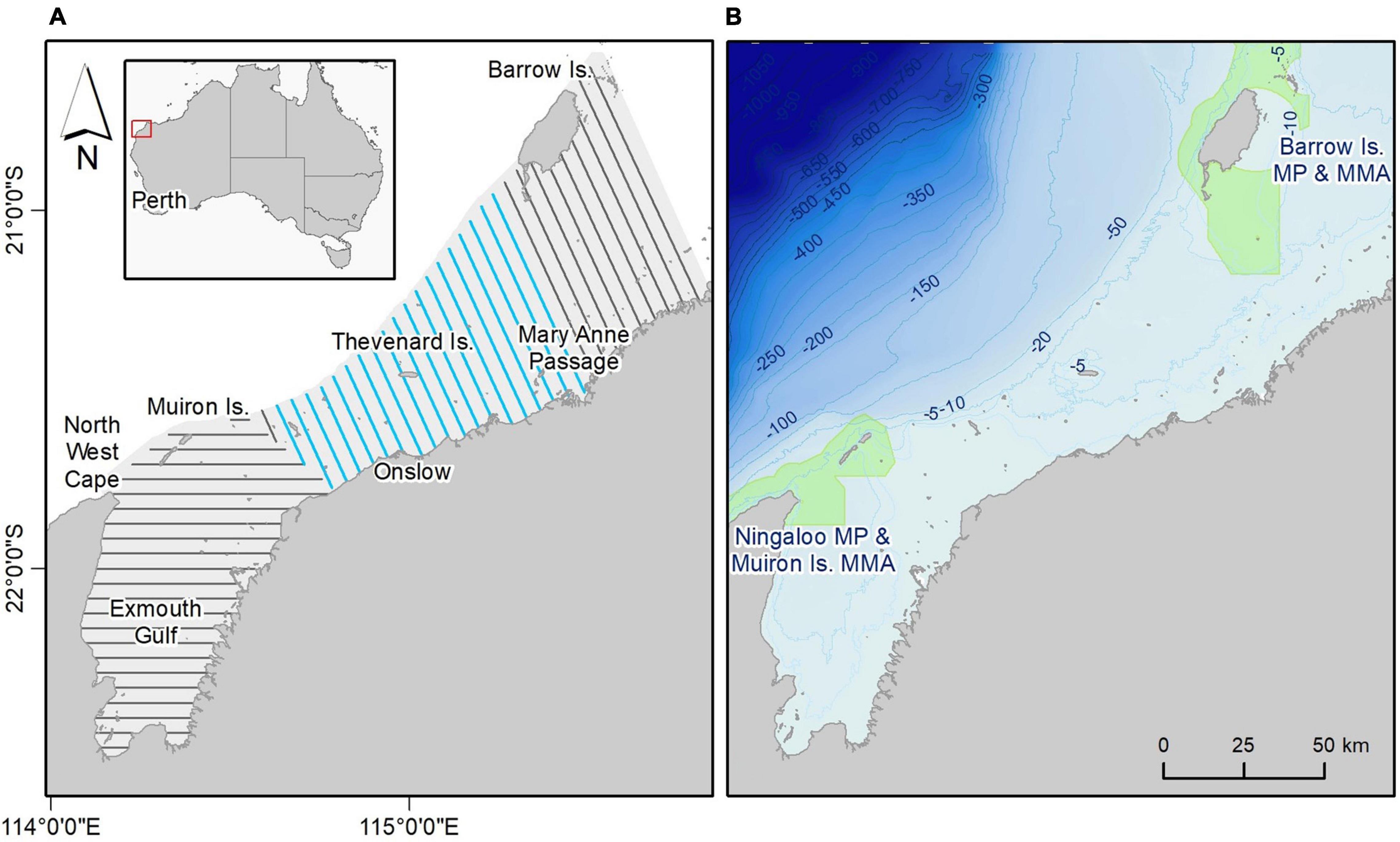
Figure 1. Study area. (A) Location (inset) and study area (shaded) with survey transect lines; repeated transects shown in blue. (B) Bathymetry and Marine Protected Areas (MPAs), shown in green (MP, Marine Park; MMA, Marine Management Area).
Materials and Methods
Study Area
Our study area is approximately 1,200 km north of Perth, in the western Pilbara inshore region (Figure 1). The 10,600 km2 area encapsulates the wide protected embayment of Exmouth Gulf and coastal waters north to the north-east of Barrow Island, and out to the 20 m isobath (Figure 1A). An ancient, submerged coastline (exposed during the Last Glacial Maximum), the study area is situated on the inner shelf and is predominantly flat and shallow (Wilson, 2013). Depth gradually increases at the outer, seaward, edge of the study area with the first drop in depth at the 20 m bathymetric contour (Figure 1B). Habitats in the area include patchy mangroves, broad expanses of intertidal algal mats (in the south), ephemeral seagrasses, and both intertidal (fringing islands and on limestone platforms) and subtidal tropical coral communities. Ningaloo Marine Park (MP) and Muiron Island Marine Management Area (MMA) (both within the Ningaloo Coast World Heritage Area) are in the south-west, and Barrow Island MP and MMA are in the north-east (Figure 1B). Strong tidal currents between the North West Cape and Muiron Islands flush internal waters of Exmouth Gulf, which maintains normal oceanic salinity levels and facilitates an exchange of nutrient rich waters and associated fish assemblages between deep and shallow environments. The major currents that facilitate productivity in the western Pilbara are the Holloway Current and the Leeuwin Current (Wilson, 2013), the former feeding into the latter. The southward flowing Leeuwin Current is WA’s prevailing oceanographic feature. It is strongest in May–July and during La Niña years; weakest between October to March and during El Niño years (D’Adamo et al., 2009). The northward Ningaloo Current is dominant on the inner shelf from September to mid-April and supports the retention of planktonic biomass in the ecosystem (Taylor and Pearce, 1999). Seasonal cyclonic activity is high between October and March and is expected to increase because of climate change (Abbs, 2012).
The study area encompasses a large portion of the newly recognised Ningaloo Reef to Montebello Islands Important Marine Mammal Area (IMMA), identified by the IUCN for cetacean biodiversity including coastal dolphins.
Aerial Survey
Dolphin sightings were opportunistically recorded (as a second priority taxa) during aerial surveys designed for dugongs, following the protocol of Marsh and Sinclair (1989) as refined by Pollock et al. (2006). Ten surveys were conducted over a four-year period: May, July, October, and December 2012, and then May (Austral autumn) and October (Austral spring) in 2013, 2014, and 2015. Survey flights were conducted using a fixed-high-wing, six-seater Partenavia P68B aircraft, at an altitude of 500 ft (152 m) above sea level, and at a groundspeed of 100 knots. The flights were restricted to weather conditions suitable for detecting dugongs and, by default, coastal dolphins (wind speeds ≤10 knots). A systematic, parallel strip transect survey design followed the same transects used for previous dugong studies (Preen et al., 1997; Prince et al., 2001; Hodgson, 2007) (Figure 1A). Three blocks were flown within the study area – Exmouth Gulf, Onslow and a repeated area within the Onslow block that included the development footprint for which the dugong monitoring programme was conducted.
Experienced observers and a double platform approach [i.e., two observers on either side of the aircraft as outlined by Marsh and Sinclair (1989) and Pollock et al. (2006)] were used to maximise accuracy and enable corrections for perception bias in recording dugongs. A block-out curtain and separate intercom systems visually and acoustically isolated observers on the same side of the aircraft so that sightings were made independently. Marker rods attached to pseudo wing struts on both sides of the aircraft delineated 200 m (at ground level) strips consisting of four 50 m zones. Observers focussed on recording sightings within the strip, however, if they saw any animals as well as those inside (i.e., within the narrow space between the aircraft and the first marker rod) and just outside (i.e., beyond) the strip they also recorded those (largely to ensure observers weren’t tempted to record sightings as within the strip when they were not). Sighting data were recorded by observers in real time onto a portable two-track audio recorder and later processed using time stamps and zone information to merge double sightings from the teams of two observers. Sighting conditions (glare, visibility, cloud cover, and sea state) and effort data were entered into a customised iPad app (Marsh, 2015) by the survey team leader approximately every 2 min or whenever conditions changed. The location of the aircraft was recorded by two Garmin eTrex 10 Global Positioning System units every 2 s (up to 15 m positional accuracy).
Dolphin Sightings
For each dolphin sighting, the following data were recorded: taxon (species or genus); taxon identification certainty (as “certain,” “probable,” or “guess”), group size; calf presence; transect zone (“low,” “medium,” “high,” or “very high” – each being a consecutive 50 m further away within the observed strip width); and turbidity on a scale of 1–4 (“1”: clear water, shallow depth and the seafloor is clearly visible; “2”: variable water clarity, variable depth range and the seafloor is somewhat visible; “3”: clear water, depth greater than 5 m and the seafloor is not visible; “4”: turbid water, variable depth range and the seafloor is not visible; adapted from Pollock et al., 2006). Certainty in taxon identification was based on morphological characteristics and surfacing behaviour of the animal, and influenced by the quality of the observation which can be affected by factors including distance, duration of animal availability, aspect and sun reflection. Surveys were conducted in passing mode, meaning that the pilot did not circle back over animals to confirm species or group size estimates. Consistency amongst observers was achieved through pre-survey training and continual peer-moderation. We have considered dolphin species recorded as “unknown” or a “guess,” as unidentified dolphin species. Bottlenose dolphin sightings were assumed to be of Indo-Pacific bottlenose dolphins because the study area was bound to the 20 m bathymetric contour. A genetic investigation off northern WA by Allen et al. (2016) identified Indo-Pacific bottlenose dolphin occurrence within the 50 m bathymetric contour, and common bottlenose dolphin (Tursiops truncatus) occurrence beyond it. It is possible that common bottlenose dolphins were also encountered but in such low proportions that they would be unlikely to skew the data.
Dolphin locations were adjusted from the aircraft’s position on the transect line, to the middle of the zone in which they were recorded, and plotted in ArcGIS v 10.1 (ESRI, 2012), assuming dolphins were directly abeam of the aircraft at the time recorded. Dolphins recorded just “inside” or “outside” of the strip were retained for analysis with their location adjusted to 25 m inside or outside of the strip, accordingly. For each species recorded, we created point distribution maps with depth data at lowest astronomical tide (LAT) (mean tidal range at Onslow = 1.8 m) (Whiteway, 2009) to present sighting locations. We went on to generate habitat suitability models for humpback and bottlenose dolphins, as they had high enough sample sizes to allow us to do so.
Environmental Data
All spatial data processing was carried out using ArcGIS v. 10.1. We generated a series of raster data layers for the study area at 500 × 500 m resolution. This resolution was chosen to keep a fine scale sensitivity when exploring distances from land and islands. Our five static environmental predictors were: depth, seabed slope, distance from the 20 m bathymetric contour, distance from intertidal areas and distance from major water ways (i.e., rivers and creeks). Our six dynamic predictor data layers were sea surface temperature (SST), ocean fronts, and chlorophyll a (chl-a), for both May and October. We assumed that because dolphins are apex predators their distribution is highly influenced by prey availability. In the absence of prey data, we used variables that could act as proxies for prey distribution. For instance, depth affects temperature, light attenuation, salinity, and the presence of benthic primary producers; and associated seabed slope can reflect upwelling areas that attract fish and cephalopods (Cañadas et al., 2002; Hastie et al., 2004; Redfern et al., 2006; Elith and Leathwick, 2009; Garaffo et al., 2011; Blasi and Boitani, 2012; Azzellino et al., 2012). Depth (m LAT) was sourced from the Whiteway (2009) gridded bathymetry data (0.0025 decimal degree resolution). We calculated slope from depth using the “Slope” tool, and distance from the slope at the 20 m contour (an ancient coastal feature, and most prominent bathymetric feature in the study area) using the “Euclidean distance” tool. As others have found, Australian coastal dolphin distribution to be influenced by distance from the mainland coast, islands and river mouths (Corkeron et al., 1997; Parra et al., 2006b; Hunt et al., 2020; Bouchet et al., 2021; Haughey et al., 2021). We calculated these distances at the mean high water mark from Geoscience Australia (2004)’s coastline and Crossman and Li (2015)’s surface hydrology data using the “Euclidean distance” tool. As the resulting “distance to islands” and “distance to the mainland” data were confounded when used separately in preliminary models, we created an alternative single data layer “distance to intertidal areas.” Intertidal areas were derived using the Euclidean Distance tool in GIS and the Geoscience Australia, 2004 “coast” dataset. Intertidal areas refer to areas around the mainland, islands and shoals that are exposed at low tide. Sea surface temperature (SST), ocean fronts (“fronts”) and chl-a are dynamic variables that can reflect seasonal pulses of productivity (Redfern et al., 2006). SST can be highly dynamic in coastal environments, with a seasonal effect on dolphin distribution (Dawson et al., 2008; Becker et al., 2010, 2012; Garaffo et al., 2011). We investigated the influence of SST within and between years because seasonal SST has been suggested as a driver of dolphin distribution in the offshore waters adjacent to our study area (Sleeman et al., 2007), and bottlenose dolphin distribution is influenced by El Niño-Southern Oscillation (ENSO) in southern WA (Sprogis et al., 2017a). We obtained daily SST at 1 km resolution from the JPL MUR MEaSUREs Project (2015), using Marine Geospatial Ecology Tools (MGET) (Roberts et al., 2010) and created a mean raster to represent each survey period. Exploratory analysis showed that SST in May and October 2015 (a strong El Niño year) were anomalous, with lower SST in May compared to other years and a convergence in SST between the 2 months (see Supplementary Material). Based on this, we created a mean of “non-El Niño” year data for May and October of 2012, 2013, and 2014, and kept May and October 2015 separate. Fronts were generated using the “focal statistics” tool calculating standard deviation in SST between grid cells. We sourced chl-a from NASA Goddard Space Flight Center (2014) using MGET (Roberts et al., 2010), while recognising that chl-a data are based on algorithms for the offshore oceanic environment and not validated for coastal waters.
Maximum Entropy Modelling
We created distribution models for humpback and bottlenose dolphins using the Maximum Entropy (“MaxEnt”) software (Phillips et al., 2004, 2006), a machine learning method used in a wide range of ecological applications that performs well in its predictive accuracy (Elith et al., 2006). MaxEnt is a technique that uses presence-only data, along with background data, to model the probability of species presence, conditioned by environmental constraints (Phillips et al., 2004; Elith et al., 2011). We treated our data as presence-only because we knew there to be a high level of pseudo-absences, having removed the unidentified dolphin species sightings. MaxEnt generates background data in place of absence data by sampling environmental variables from random points throughout the landscape. MaxEnt’s underlying theory and assumptions are described in detail elsewhere (Phillips et al., 2006; Phillips and Dudik, 2008; Elith et al., 2011). MaxEnt uses an automatic regularisation setting that has been fine-tuned to suit the number of feature types and sample locations (Phillips et al., 2006). As with other forms of machine learning, regularisation is used to prevent models from being overfit by adding a complexity penalty to the loss function. Through regularisation and optimisation, a series of iterations are run which achieves high model gain. High gain reflects that the model is a good fit to the data, which is like the “deviance” goodness-of-fit measure used in general additive models (Phillips et al., 2004). During this process, MaxEnt generates a probability distribution and populates this information into cells of a geographic grid, based on the sampled background data.
We created a static model (i.e., without dynamic variables) for both humpback and bottlenose dolphins, which we used to compare distribution patterns between the species. In addition, we ran May and October, non-El Niño and El Niño models for bottlenose dolphins to investigate seasonal variation and response to dynamic variables. We were unable to create seasonal models for humpback dolphins, as there were fewer data available for sufficient sample sizes after subsetting. We accounted for greater sampling effort in the repeated “Onslow” block (Figure 1B) by including a spatial bias grid (Phillips et al., 2006, 2009). Cells within the repeated block (which had twice the survey effort) were assigned a value of “2” and all other cells were assigned a value of “1.”
Maximum Entropy default settings can fit features (combinations of environmental variables with alternative transformations and model terms) to the model depending on the training data sample size (Phillips et al., 2004; Elith et al., 2006). While MaxEnt default settings perform well, Merow et al. (2013) suggests that user refine these based on their data to achieve clear and simple models and avoid over-fitting. We incrementally tested various combinations, checking the output curves to see that they were not overly complex for the sample sizes available (as reported in the section “Results”). We chose to specify linear, quadratic and product features for our final models, and deselected threshold and hinge features, which allow for steps in the fitted function. We set the prevalence and regularisation at the default value of 0.5, which represents a 50% chance of species occurrence in any cell (Phillips et al., 2004; Elith et al., 2006). The raw sightings data showed that humpback and bottlenose dolphins were broadly distributed throughout the study area. As such, we deemed the default setting of 0.5 to be appropriate for this preliminary study, with each cell having an equal chance that a humpback or bottlenose dolphin could be present. Each model was run using sampled background data set to a maximum of 10,000 random points over a maximum of 500 iterations for 1,000 bootstrapped replicates. This resampled, with replacement, 25% of dolphin data as test data, thereby conserving the data available for training purposes. Each final model was the mean of all replicates.
Our model outputs consist of estimates of habitat suitability, environmental variable contributions and response curves. Mean relative habitat suitability, as a probability distribution from zero to one based on favourable environmental conditions across the study area, was generated in logistic output. Environmental variable contributions (relative to each other and expressed as a percentage) to the model were determined during regularisation. We used non-marginal response curves which are clearer to interpret than marginal response curves as they reflect the influence of the variable itself, and not the interactions it has with other variables. Diagnostic plots of commission and omission rates were used to assess model performance. The Receiver Operating Characteristic (ROC) curve represents sensitivity (true positive rate) against the specificity (fraction of negative instances) (Phillips et al., 2006) and is reflected by the Area Under the Curve (AUC) metric. The AUC metric ranges from 0 to 1 in presence-absence models. An AUC of 1.0 is unable to be reached by MaxEnt models because they are trained on background (a closely related alternative to pseudo-absence) data (Phillips et al., 2006; Elith et al., 2011). The models present a landscape of potential distribution, rather than a “true” distribution. An AUC score of >0.5 suggests that a model performs better than random (i.e., when it has 50% chance of being correct) (Fielding and Bell, 1997). We judged model performance following Hosmer and Lemeshow (1989): <0.5 = none; 0.5–0.7 = poor; 0.7–0.8 = acceptable; 0.8–0.9 = excellent; >0.9 = outstanding. This aligns with Elith (2000)’s assertion that MaxEnt models >0.75 have potentially useful management applications. The omission plots show training omission rate and predicted area as a function of the cumulative threshold of suitable habitat. A good model, in terms of omission, is indicated by the training data trend line falling below the predicted rate (Phillips et al., 2006).
Results
Effort and Sighting Conditions
We surveyed 21,156 km of transect line during May (9,116 km), July (2,279 km), October (7,482 km), and December (2,279 km) from 2012 to 2015, with July and December surveyed only in 2012 (Table 1). Fewer transects (i.e., those in the repeat block) were flown in October 2014 and 2015 due to weather constraints. The aerial surveys were conducted in good weather conditions (wind speed mode = 5 knots; cloud cover mode = 0 okta; Beaufort sea state mode = 2; visibility mode = >10 km) (Supplementary Table 1). Glare was arguably the most limiting sighting condition (mode = 3 on a scale of 1–4), largely dependent on the time of day.
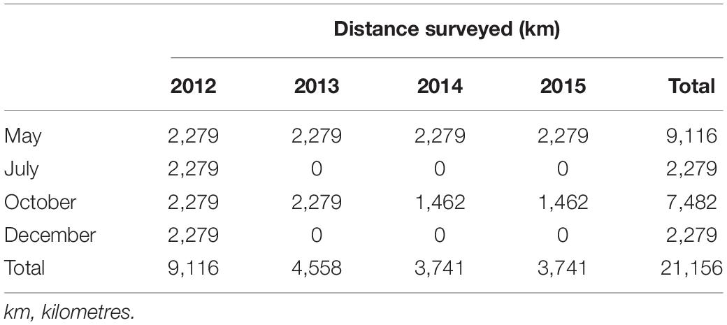
Table 1. Transect effort, by month and year.
Dolphin Sightings
A total of 1,169 dolphin sightings (i.e., groups, which may consist of one or more individual animals) were recorded over the full survey period (Table 2 and Figure 2). Bottlenose dolphins were the most frequently encountered species (n = 661; 55.7%; rate of 2.90 sightings/100 km), seen across all water depths measured at LAT (Geoscience Australia, 2004) (min – max LAT = 0–37 m; mean LAT = 10.5 m). A quarter of all sightings (n = 290; 24.8%; rate of 1.27/100 km) were of unidentified dolphin species, also seen across all water depths. Humpback dolphins constituted 16.3% of the sighting data (n = 191; rate of 0.83/100 km), their locations trending toward shallower water depths (min – max LAT = 0–24 m; mean LAT = 10.5 m).
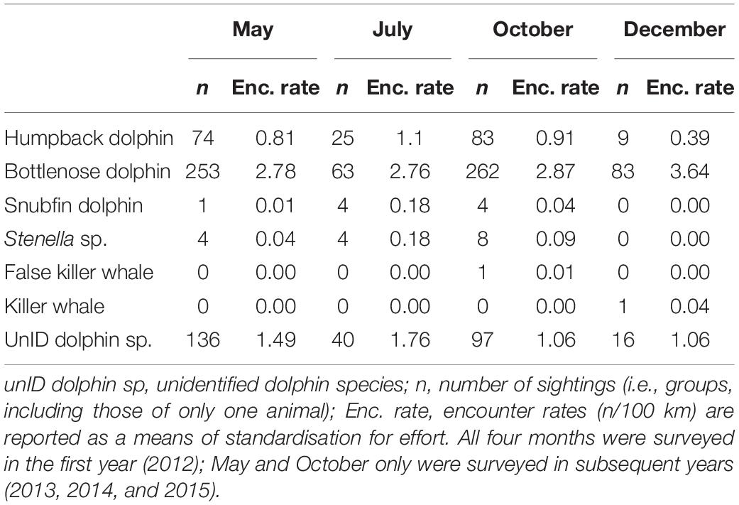
Table 2. Sighting summary for each dolphin species, including those recorded as unknown, across months when surveys were undertaken.
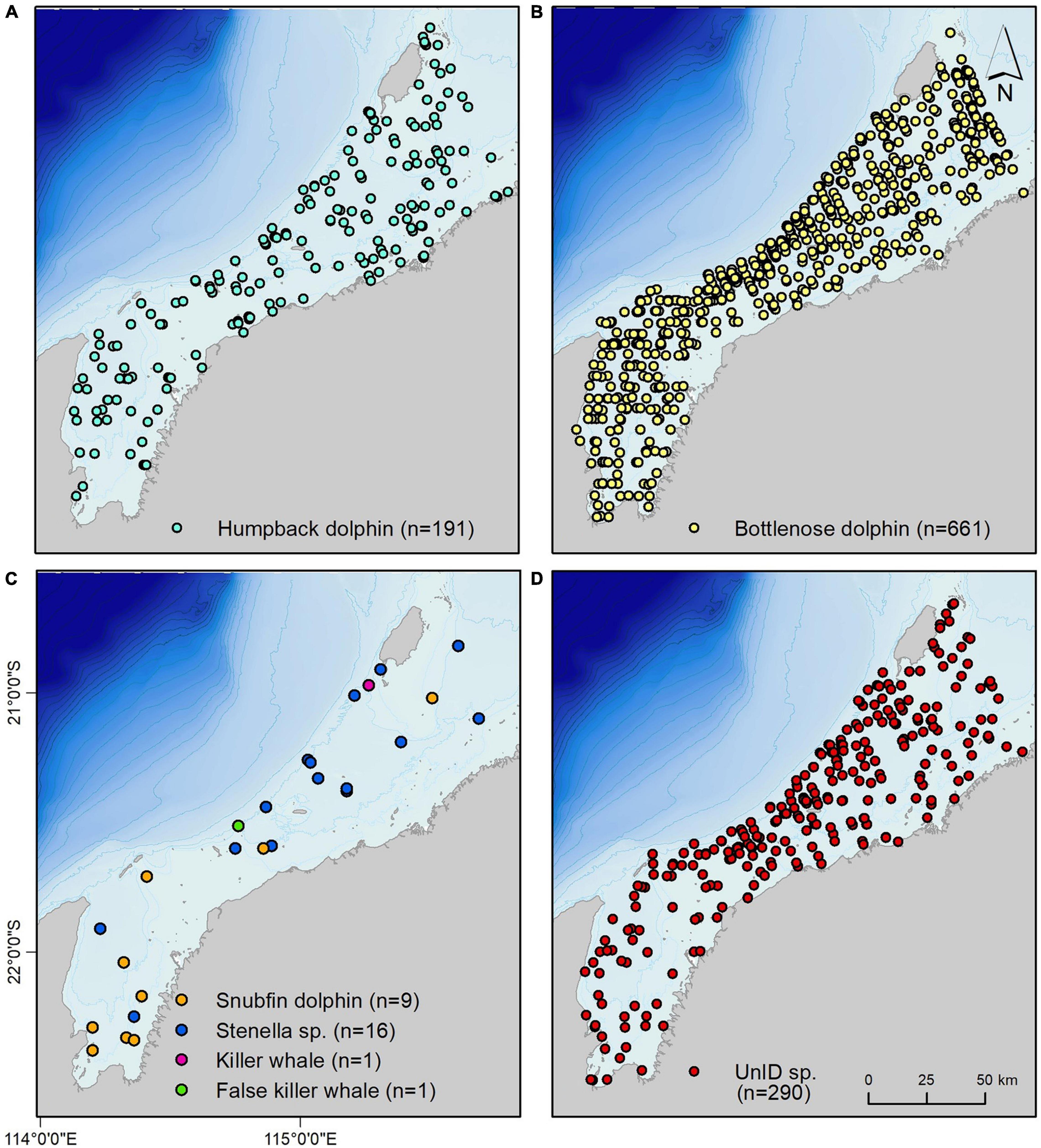
Figure 2. Distribution of (A) humpback dolphins; (B) bottlenose dolphins; (C) less commonly encountered species: snubfin dolphins, Stenella sp; killer whales and false killer whales; and (D) unidentified species (unID sp.), for the full four year survey program. n, number of groups (totalling 1,169). Species were identified with certain or probable levels of certainty (see Table 3).
The remaining sightings were of snubfin dolphin (n = 9; 0 certain; all probable), Stenella sp., (n = 16; 4 certain; 12 probable), killer whale (Orcinus orca, n = 1; certain) and false killer whale (Pseudorca crassidens, n = 1; certain) groups (Tables 2, 3). Snubfin dolphin sightings were mainly within Exmouth Gulf, in depths of 5 m or less (min = 0 m LAT; max = 12 m LAT; mode = 5 m LAT). Most (n = 13). Stenella sp. sightings were in the north-eastern portion of the study, as were killer and false killer whale sightings. A group of two adult killer whales were recorded in December near Barrow Island in 14 m LAT depth. A group of false killer whales (n = 50–60 with calves present) was recorded in October, west of Thevenard Island in 9 m LAT water depth.
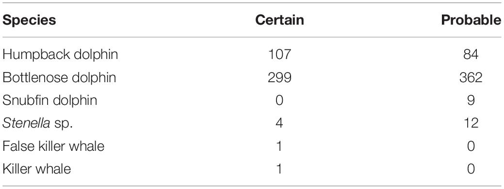
Table 3. Number of sightings that were certain or probable for each species.
Maximum Entropy Models
Model Performance
Models had poor to excellent performance, following Hosmer and Lemeshow (1989). Mean AUCs ranged from 0.63 ± 0.01 (i.e., the bottlenose static model) to 0.82 ± 0.03 (i.e., the bottlenose May El Niño model), with an improvement in model performance when dynamic variables were incorporated (Table 4). ROC plots show AUC trend lines above 0.5 for both training and test data, and mean omission rates align with those predicted (see Supplementary Material) for all models, excluding the bottlenose May El-Niño model for which the rate fell under. These diagnostics reflect the preliminary nature of the models and highlight the need for ground validation.
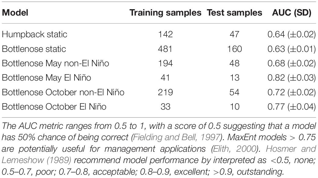
Table 4. Table AUC, area under the curve; SD, standard deviation.
Environmental Variables
The proportion that each variable contributes to the humpback dolphin model is more even compared to that of the static bottlenose dolphin model. “Distance to intertidal areas” had the largest contribution (27.3%), and “slope” had the least (14.6%) (Table 3). Response curves clearly indicated that humpback dolphins were most likely to be present in shallow (<10 m) and flat areas (Figures 3A,B). Which aligns with existing knowledge for the species at other locations. A non-monotonic relationship exists with distances to intertidal areas and waterways (Figures 3C,E). There is a slightly higher probability of humpback dolphin presence nearer to intertidal areas (Figure 3C), which is supported by the maps (Figure 4A). Humpback dolphin presence had a concave response to major water ways (Figure 3E), with highest probability of occurrence at greater distances. The weakest response for humpback dolphin presence was with distance from the 20 m isobath (Figure 3D), indicating that it does not strongly influence their distribution.
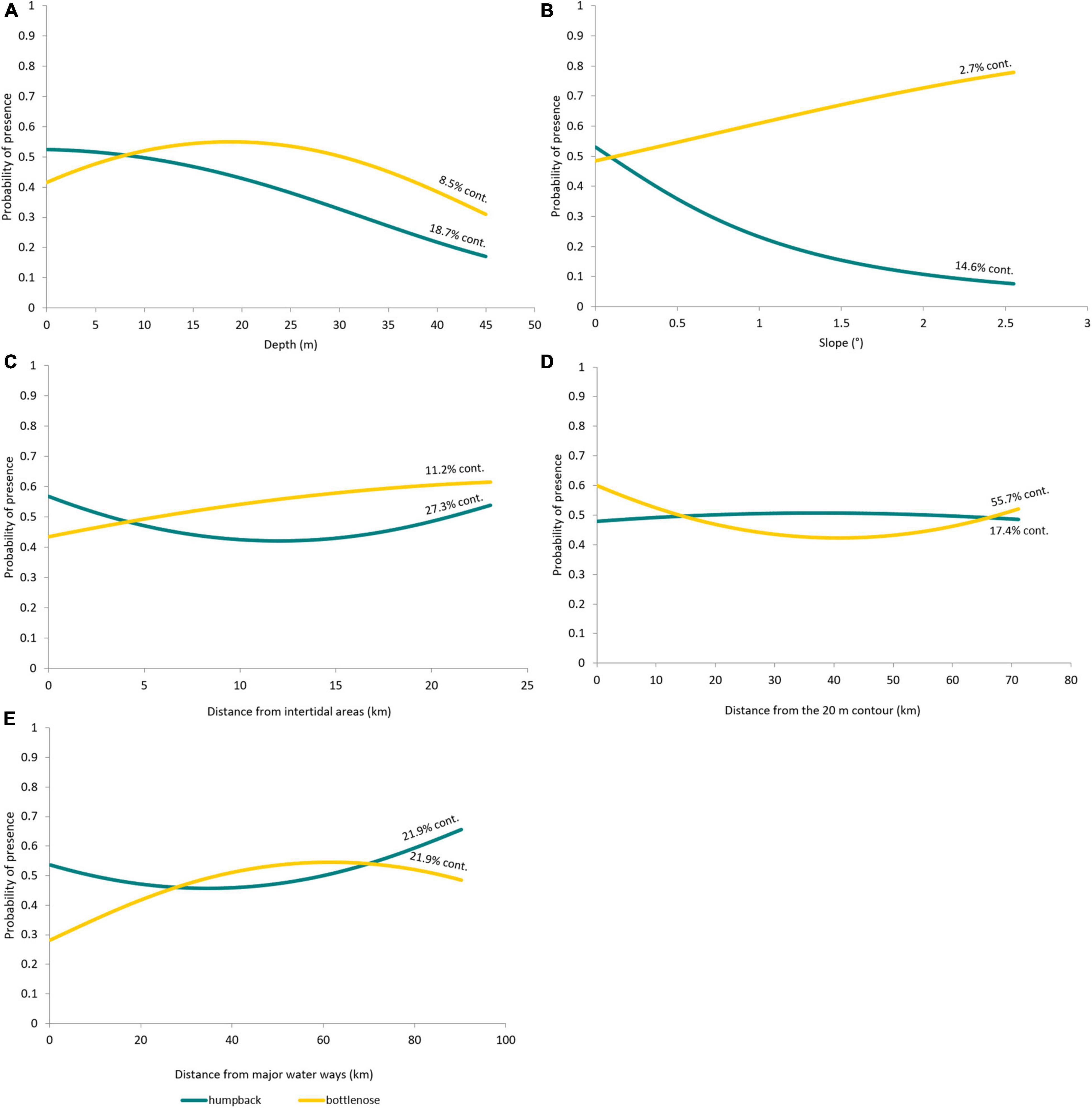
Figure 3. Probability of humpback (teal) and bottlenose (gold) dolphin presence as a response to static environmental variables: (A) Depth; (B) Slope; (C) Distance from intertidal areas; (D) Distance from the 20 m isobath, and (E) Distance from major water ways. m, metres; km, kilometres. Percent contribution (% cont.) of each variable to the humpback and bottlenose models are presented within the figure, alongside each response curve.
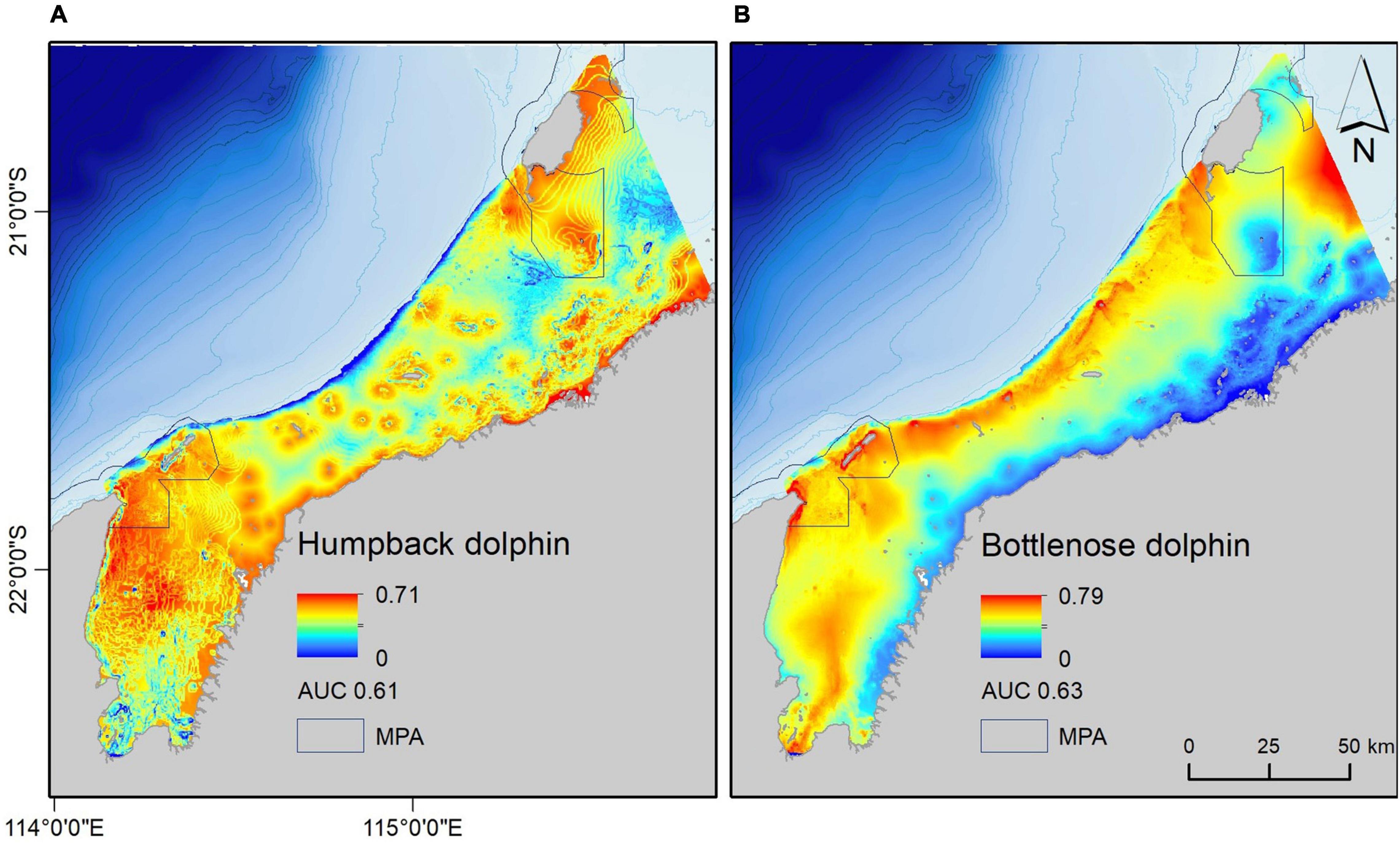
Figure 4. Habitat suitability for (A) humpback and (B) bottlenose dolphins at 500 × 500 m grid cell resolution. Habitat suitability across the study area ranged from 0 to 0.71 for humpback dolphins and 0 to 0.79 for bottlenose dolphins. Area under the curve (AUC) indicates model performance. Marine Protected Areas (MPAs) are outlined.
The static bottlenose dolphin model was influenced most by “distance from the 20 m isobath” (55.7%) and least by “slope” (2.7%) (Figures 3B,D and Table 5). Bottlenose dolphins’ response to distance from the 20 m isobath is non-monotonic, although their probability of presence is highest near to it. The response curves show, in contrast to humpback dolphins, that bottlenose dolphins are more likely in waters that are deeper (10–25 m) and further away from intertidal areas (Figures 3A,C).
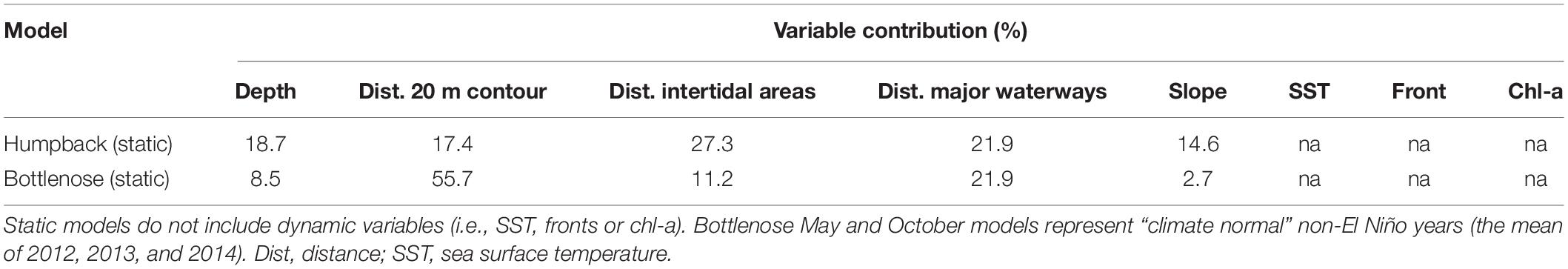
Table 5. Environmental variable contribution, relative to each other and expressed as a percentage, toward each model.
Seasonal and Climatic Variation in Bottlenose Dolphin Distribution Models
The variable contributions to bottlenose dolphin models are inconsistent across seasons and non-El Niño/El Niño years (Table 6). Response curves from the seasonal models supported the theory that SST influences bottlenose dolphin distribution (Figure 5). In May of non-El Niño years, waters are warmer (∼25.5–28.5°C during our study period), and bottlenose dolphins show a positive response to SST and SST fronts (Figures 5A,C). Although May SST is reduced (∼23.5–27°C) when El Niño is in effect, bottlenose dolphins retain this positive response. Conversely, there is a negative response to SST in October when waters are cooler (∼23.5–25.5°C during non-El Niño; ∼24–27°C during El Niño) (Figures 5B,D). While this is reflected by the dolphins’ negative response to SST fronts in non-El Niño October, response to fronts in El Niño October is positive (Figure 5D). Mapped output for El Niño October also diverges by showing the interior of Exmouth Gulf (see Supplementary Material) to be more important than the area near the 20 m isobath.
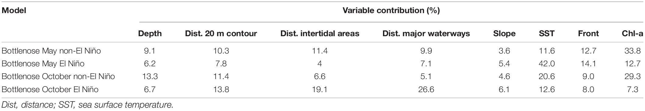
Table 6. Environmental variable contribution, relative to each other and expressed as a percentage, toward each bottlenose dolphin seasonal model.
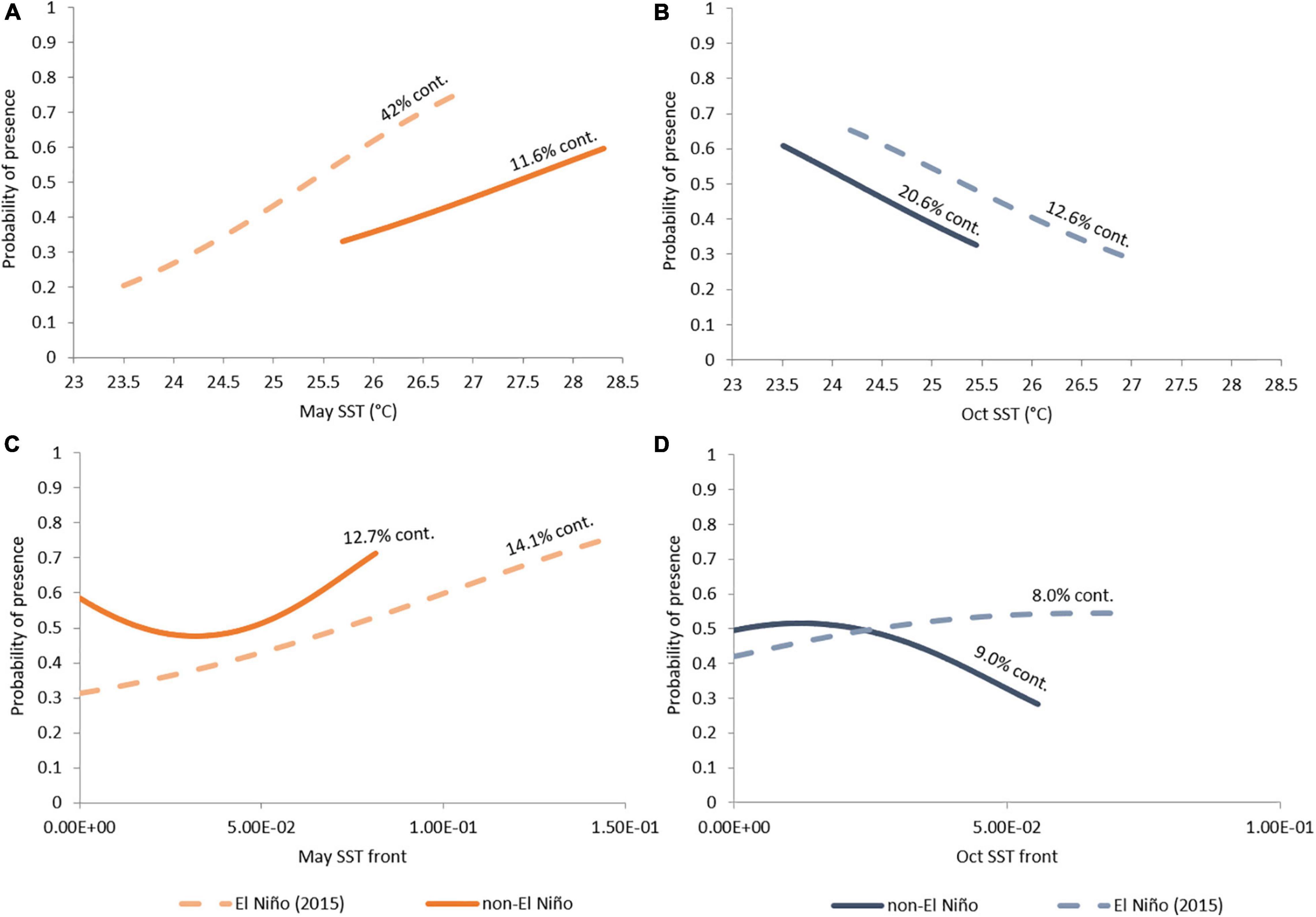
Figure 5. Probability of bottlenose dolphin presence as a response to sea surface temperature (SST) in (A) May and (B) October, and to SST fronts in (C) May and (D) October, during El Nino (2015, dashed line) and non-El Nino years (2012, 2013, and 2014, solid line).
Although chl-a appears to have a strong influence on both seasonal bottlenose dolphin models (May = 33.8%; October = 29.3%), there is a negative response in each instance (Figures 6A,B).
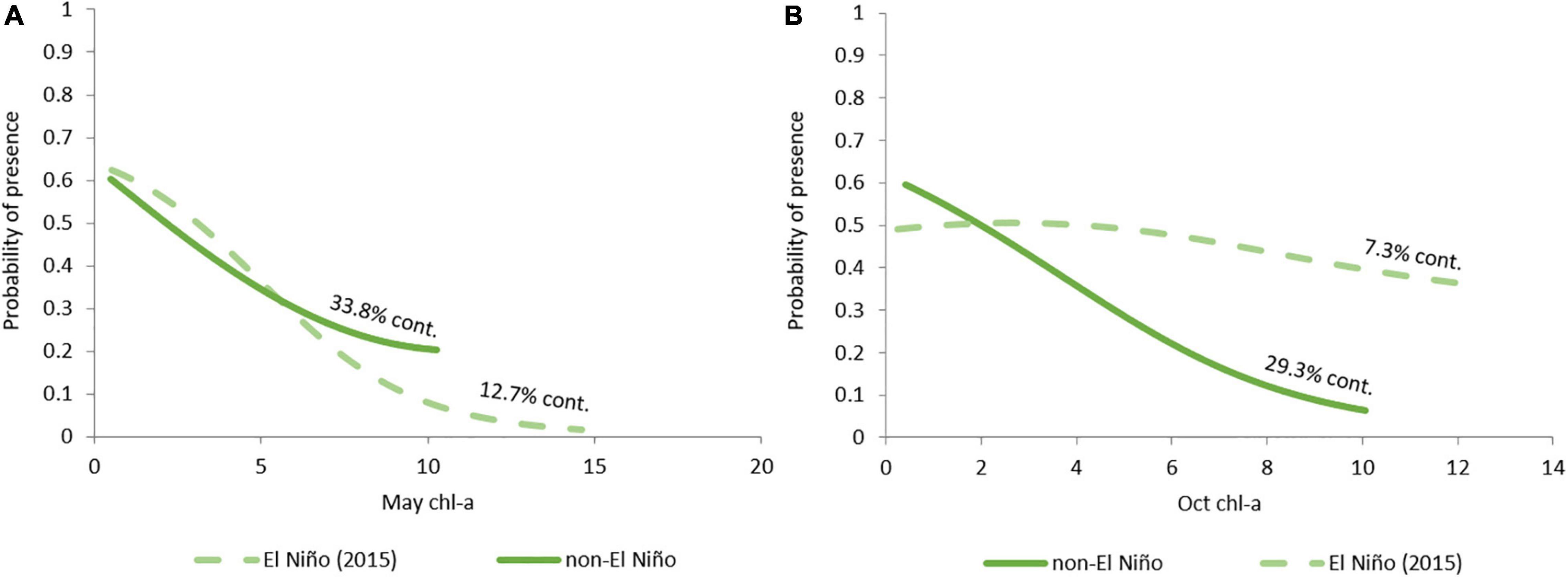
Figure 6. Probability of bottlenose dolphin presence as a response to chl-a in (A) May and (B) October, during El Nino (2015, dashed line) and non-El Nino years (2012, 2013, and 2014, solid line).
Habitat Suitability for Humpback and Bottlenose Dolphins
Mapped output suggested a clear distinction in habitat suitability between humpback and bottlenose dolphins across the area (Figure 4). The only potential areas of overlapping high habitat suitability for the two species was around the North West Cape, Muiron Islands, and south-western Barrow Island. Humpback dolphin habitat suitability was highest in shallower intertidal areas, including the coasts of offshore islands and the mainland, Barrow Island Shoals and Mary Ann Passage (Figure 4A). Most of Exmouth Gulf was also of high habitat suitability for humpback dolphins. In contrast, bottlenose dolphin habitat was most suitable at greater depths, and generally further offshore (Figure 4B).
Discussion
Situated on the inner North West Shelf, the western Pilbara coastline is inhabited by coastal dolphin species with occasional visits by pelagic species. Humpback and bottlenose dolphins are the most commonly occurring species throughout the region, and both have recognised ranges that extend further north and south (Parra and Cagnazzi, 2016; Hunt et al., 2017; Manlik et al., 2019). Partitioning the sightings data by species and season (in the case of bottlenose dolphins) and incorporating environmental variables into MaxEnt models has provided broad-scale baseline data and enabled us to identify various patterns that may guide further field study design, inform project-specific EIA and management and species-specific conservation plans.
Model Interpretation
Model output should always be interpreted with an understanding of the model assumptions and data characteristics on which they are based. Due attention should always be paid to understand model output type, level of certainty and generalisation, spatial resolution, and the accuracy and sample size of both species and predictor variable data on which the model has been based (Redfern et al., 2006; Araújo and Guisan, 2006; Jiménez-Valverde et al., 2008; Elith et al., 2011). Our maps present relative dolphin habitat suitability across the western Pilbara, based on the environmental data available to us to include in the MaxEnt models. They do not present relative density or abundance. MaxEnt maps present a probability distribution across the study area based on favourable environmental conditions (i.e., habitat suitability) (Phillips et al., 2006), in contrast to a relative index of environmental suitability based on species occurrence that can be obtained by presence-absence techniques. Also, they depict a generalised distribution which is broader than the species’ realised niche (Phillips et al., 2006; Araújo and Guisan, 2006; Hirzel and Le Lay, 2008). We also wish to highlight that they cannot be directly compared across models. The AUC score for MaxEnt models will always be penalised because the model is based on background data rather than absence data; it can never reach “1,” and “0” does not indicate absence (Phillips et al., 2006; Elith et al., 2011).
Our models provide new insight into potential humpback and bottlenose dolphin habitat suitability. The performance metrics are not high, and we suggest that the main reason for this is a lack of informative environmental variables across the study area, followed by imperfect sightings data (see section “Study Limitations”). However, at such a broadscale they are still useful for conservation and management planning (Elith, 2000). As outlined by Redfern et al. (2006) habitat models for cetaceans can be useful as a starting point for understanding distribution patterns when knowledge of a species’ ecology is lacking, which we advocate for the coastal dolphins in WA’s Pilbara region.
Important Areas for Humpback Dolphins
Across our broad study area, we have found that humpback dolphins are most likely to inhabit intertidal areas and we suggest that these could represent important habitat requiring research and conservation focus. Most areas of high habitat suitability coincided with shallow waters and coral reefs, even when far from the mainland. This aligns with findings from aerial surveys over the Great Barrier Reef Marine Park (Corkeron et al., 1997) and from smaller scale studies in the region (Raudino et al., 2018a,b; Hunt et al., 2020). Humpback dolphins are listed as conservation values that are protected within Ningaloo MP, Muiron Islands MMA and Barrow Island MMA. Further, the North West Cape, situated within Ningaloo MP, has been identified as being of habitat importance for humpback dolphins (Brown et al., 2012; Hunt et al., 2017, 2020). Our model supports these claims but also suggests that these areas are part of a group of important (and likely connected) humpback dolphin habitats, most of which are outside of protected areas. The region supports a mosaic of tropical coral reefs in shallow areas around islands and on limestone platforms, such as Barrow Island Shoals and Mary Ann Passage, and patch reefs such as those within Exmouth Gulf (Wilson, 2013). We speculate that humpback dolphins in this region prey upon reef-associated fish and cephalopods, but this is yet to be confirmed through behavioural and stable isotope studies. Within the Ningaloo MP, humpback dolphins have been observed foraging and resting near reefs (D. Hanf pers. obs.) They may also benefit from positioning themselves with access to both shallow and deep water around offshore islands and North West Cape, for opportunities to hunt prey associated with offshore currents, whilst being able to use shallow water to avoid or escape predators.
Our findings contrast with those from other areas that indicate that the primary driver of humpback dolphin distribution is proximity to river mouths (Parra et al., 2006b; Palmer et al., 2014; Meager et al., 2018) which may reflect the difference in survey scale, and the different geographic area. Northern WA has dissimilar hydrology to other areas of northern Australia (the Kimberley region of WA is more like Northern Territory and Queensland) and is an example of why that EIA should be based on locally collected species data, rather than surrogate data from other populations. As humpback dolphins have been observed foraging in rivers within the Pilbara region (e.g., Fortescue River, D. Hanf pers. obs.), this habitat could be important at a local scale and used intermittently based on tides, which would not be recorded by broadscale aerial surveys.
The relatively high habitat suitability of western Pilbara coral-fringed islands, Mary Ann Passage and Barrow Island Shoals, in addition to the North West Cape (Hunt et al., 2020), support the recent nomination of the Ningaloo Reef to Montebello IMMA. We recommend that these areas be recognised as biologically important areas (BIAs) (Australian Government, 2012a), and thus be given special attention during EIA and conservation planning. This will aid strategic planning and the development of management strategies (e.g., areas of speed restriction, placement of infrastructure, oil spill contingency planning, and climate change resilience planning).
Niche Partitioning Between Humpback and Bottlenose Dolphins
By comparing broadscale models (i.e., western Pilbara region) for humpback and bottlenose dolphins, we may have been able to recognise distribution patterns not evident at a narrower spatial extent. Resource partitioning, where species live in sympatry by taking advantage of different niches to reduce competitive pressure, has been widely observed amongst dolphins (Bearzi, 2005; Parra, 2006; Kiszka et al., 2011; Fernández et al., 2013; Heithaus et al., 2013; Cremer et al., 2018). As top-order predators, co-existence of sympatric dolphin species is likely to be enabled by spatial-temporal differences in prey preferences, diet composition and foraging strategies (Berta et al., 2015). We found bottlenose dolphin habitat suitability to be high near the slope at the 20 m isobath, whereas humpback dolphin habitat suitability was highest around intertidal areas. Similar spatial separation between the two genera exists elsewhere (Stensland et al., 2006; Palmer et al., 2014). Humpback and snubfin dolphins also exhibit resource partitioning in areas where they co-occur (Parra, 2006). Separation could reflect differences in feeding strategies and risk-taking behaviour, with bottlenose dolphins exhibiting a high level of plasticity throughout their range (Cribb et al., 2013), whereas humpback dolphins have a higher site fidelity (Brown et al., 2016; Meager et al., 2018). Capture-recapture studies at the North West Cape demonstrate that bottlenose dolphins display a low site fidelity, often venturing outside of the study area while humpback dolphins show a high site fidelity with high recapture rates (Hunt et al., 2017; Haughey et al., 2020). Slopes are often important foraging areas because prey is usually in high abundance (Hastie et al., 2004). The 20 m isobath marks the end of the inner shelf after which it gradually descends to 100 m. These waters between 20 and 100 m are deep are open to oceanic currents which transport zooplankton and finfish. Furthermore, cephalopods in high abundance (Jackson et al., 2008), representing an alternative foraging area which bottlenose dolphins may take advantage of to reduce competition with humpback dolphins.
Despite partitioning across the region, there were overlaps of suitable habitat for both species at certain locations. There could be a dietary divergence between the two species at these habitats, which has been found to occur with other dolphin species (Bearzi, 2005). More likely though, it could reflect plentiful prey availability at these sites. These areas of overlap may support higher productivity, greater prey species biomass or diversity at times. For instance, mixed species groups of humpback and bottlenose dolphin groups have been recorded at the North West Cape, where offshore and inshore waters are channelled and mixed (Brown et al., 2012; Hunt et al., 2017). This is plausible as both species are “opportunistic-generalist feeders,” consuming a wide range of benthic and pelagic fish and cephalopod species (Amir et al., 2005; Parra and Jedensjö, 2014; McCluskey et al., 2016; Smith and Sprogis, 2016; Sprogis et al., 2017b). As there are many unresolved questions, targeted observational studies are required to understand foraging strategies and the mechanisms underlying mixed species group formation and behaviour (Syme et al., 2021).
Seasonal Variation in Bottlenose Dolphin Distribution
We found that bottlenose dolphin distribution is influenced by dynamic variables and theorise that response to warmer SST in May represents a shift in prey availability driven by the Leeuwin Current. A similar pattern for bottlenose dolphins was reported by Sleeman et al. (2007), with highest dolphin abundance between March and May in the area immediately offshore to our study area. This could also coincide with Sprogis et al. (2017a)’s finding that bottlenose dolphin distribution shifted offshore, toward the Leeuwin Current, during an El Nino period when the current is suppressed. Such plasticity and responsiveness to changes in environmental conditions may also be a driver of low bottlenose dolphin site fidelity at the North West Cape (Haughey et al., 2020). The response of bottlenose dolphins to SST was largely consistent between non-El Nino and El Nino years, but the mapped output indicates a more marked variation in habitat suitability which could be further explored. It is important to emphasise that the models present general patterns at a broadscale level. Bottlenose dolphins were found throughout the study area, yet the models suggest a potential preference to deeper areas which we suggest is driven by offshore oceanography that influences prey availability. Finer scale studies may find variation within the population. For instance, Sprogis et al. (2018) found female bottlenose dolphins to prefer deeper water depths than males during summer and spring. These hypotheses could be investigated through targeted in situ studies involving the collection of behavioural data and biopsy samples for stable isotope analyses.
Our ability to consider seasonal and annual variability highlights the strength of multi-year studies and cautions on single-year studies as there may be various confounding issues that can affect animal distribution and associated conclusions regarding presence and habitat. Longer-term studies (i.e., decadal) in the future would be preferable, to capture the effects of climatic events such as the La Nina event of 2011, which contributed to a marine heatwave and caused large-scale fish and benthic primary producer die-off, as well as the displacement of tropical species (Pearce and Feng, 2013). Sprogis et al. (2017a) were able to clearly detect abundance decline in their study area during an El Nino winter. Cyclones and associated flooding, prominent in the Pilbara region between October and March, are also set to increase with climate change (Abbs, 2012). As flood events effect coastal dolphin distribution (Cagnazzi et al., 2020), long-term data (ideally and decadal) are needed to build predictive models.
Other Dolphin Species
Snubfin dolphin occurrence in the Pilbara region is a subject of some conjecture and our study has not been able to confirm their presence. This location is approximately 650 km south-west of their recognised range (IUCN SSC Cetacean Specialist Group, 2017; see Supplementary Material). Occasional and compelling anecdotal reports of snubfin dolphin presence in the Pilbara region exist since at least 1995 when a Department of Conservation and Land Management Wildlife Officer P. Mawson filed an official memorandum describing his certainty in sighting of two or three individuals at the North West Cape. Allen et al. (2012) collated several reports including those made by seasoned marine mammal scientists. Nine snubfin dolphin sightings were recorded by observers during our surveys. However, none of these were made with certainty in species identification and there were no clear recaptures between front and rear observers. Misidentification between dugongs and snubfin dolphins can sometimes occur, particularly during aerial surveys platforms (Dunshea et al., 2020). It is worth noting that no opportunistic snubfin dolphin sightings have been made by marine mammal researchers conducting other boat-based studies in Exmouth Gulf and around NW Cape in recent times, which may be an indicator of their scarcity in the area (i.e., Hunt et al., 2017; Raudino et al., 2018a; Bejder et al., 2019; Haughey et al., 2020; Sprogis et al., 2020a,b). We suggest that vagrant individuals may occasionally occur within our study area. Parts of Exmouth Gulf (where most of our sightings were made), share similar habitat characteristics to Roebuck Bay, i.e., large shallow embayment fringed by mangroves and intertidal salt/mud flats connected to deep oceanic waters with a complex of seagrass, reef and sponge beds forming a rich prey environment (Australian Government, 2012a). Further studies are needed to investigate the species’ full extent of occurrence in Western Australia, including whether small discrete populations exist within the Pilbara region. Such information is required for their full assessment as a threatened species under the EPBC Act and is a critical information gap in marine spatial planning.
Pelagic species are likely to move into our study area from adjacent deeper waters where key ecological features (narrow shelf, canyons and the Exmouth plateau) facilitate upwelling and enhance local productivity (Australian Government, 2012a; Wilson, 2013). Stenella sp. sightings may include pantropical spotted (Stenella attenuata), and dwarf spinner (Stenella longirostris) dolphins, as North West Cape stranding records include the former (Groom and Coughran, 2012) and the latter has been identified from north WA biopsy samples (Leslie and Morin, 2018). Our killer whale sighting in December 2012 is one of the rare, documented sightings of this species in the region in summer outside of the humpback whale season when most killer whale research has been undertaken (e.g., Pitman et al., 2015). This suggests that the local population may not have a feeding niche that is as specialised as previously thought, or that resource partitioning exists with separate summer and winter groups feeding on different prey at different times (J. Totterdell pers.com.). We also recorded a large group of false killer whales, a “Near Threatened” species (IUCN, 2020), for which a paucity of data exists in Australia as well as globally (Woinarski et al., 2014). This species is generally regarded as a migratory, tropical to subtropical, deep-water, oceanic species that is sometimes encountered in neritic areas (Baird et al., 2012; Zaeschmar et al., 2014). Palmer et al. (2017) demonstrated that false killer whales may be regular visitors to coastal and estuarine environments in north Australia and that further research regarding their habitat use is warranted. As we only recorded the species once during 10 surveys, we suggest that they were likely encountered while undertaking broadscale movements and are more likely to be pelagic visitors to the coastal environment.
Study Limitations
The major shortfall of our study was the uncertainty in species identification, as a result of observers focussing on searching for dugongs as their primary target, a limited “search” time (intrinsic to all aerial surveys and particularly passing mode surveys) and the similarity in appearance of humpback and bottlenose dolphin species from aircraft. These limitations reduced the data available for modelling by 25% and constrained our choice of modelling method. However, as surveys were conducted over multiple years, we were able to pool data for “static” and non-El Niño models, which assumed that relationships did not vary across years. The bottlenose dolphin El Niño models should be interpreted with caution as they encapsulate only one season’s worth of data. The low AUCs, weak patterns in environmental contributions (apart from distance from the 20 m slope for bottlenose), and non-monotonic response curves likely reflect noise in the model. Finer scale patterns than what we have presented are likely to exist across the area, with different levels of contribution by and interaction between environmental variables. Ideally, we would have a larger dataset which we could further partition to investigate this [e.g., using sampling instances as outlined by Matthiopoulos et al. (2011) in their generalised functional response approach]. This could be achieved through the simultaneous acquisition of photographic data that would allow species identification verification.
Another limitation in our study was the lack of data on benthic primary producers and prey distributions. These predictor variables would likely provide greater information to the models which may result in clearer patterns than models based on proxies. The negative response to chl-a could be a result of the ocean colour and raises several questions. It could suggest that the data are not a good proxy for productivity in the area, or that the distribution of these dolphins is not directly driven by primary productivity. Alternatively, the data could be masked or biassed by other factors, such as turbid terrestrial run off which is characteristic of nearshore Pilbara waters. Furthermore, it could be that there is a lag between productivity and dolphin response. Ultimately, we did not find chl-a as represented by ocean colour to be useful in the models.
Conclusion
Our study exemplifies the value of maximising opportunistic datasets, particularly in areas where threatened species occur but little research effort has been undertaken for logistical (e.g., financial and access), political, or legislative reasons (Aragones et al., 1997; Dawson et al., 2008; Bejder et al., 2012). We have obtained key information for conserving and managing dolphin species in an area undergoing rising human activity. By documenting a difference in habitat use by humpback dolphins in north WA compared to other study locations, we have highlighted the importance of using locally sourced data to inform conservation management, including EIA and other decision-making processes. We have also identified new areas of importance for humpback dolphins to inform marine spatial planning. Fine-scale studies of abundance, population structure (i.e., genetics) and behaviour (i.e., how the habitat is being used) can now be targeted to areas of highest habitat suitability, enabling an informed investment of time and funding. This is important as intensive effort is required for cryptic species such as humpback and snubfin dolphins, or else low capture rates may result (e.g., Brooks et al., 2017; Raudino et al., 2018a).
We recommend that broadscale surveys continue over time, to monitor temporal trends and increase the sightings dataset. With more data available over time, we can build more sophisticated models (Redfern et al., 2006), further investigate geographic or temporal variation (e.g., Matthiopoulos et al., 2011) and construct robust predictive models for times periods or places outside of those surveyed. Future surveys would benefit from the collection of high-resolution digital images for species identification verification, either via unoccupied aerial vehicles (UAVs) or cameras mounted to occupied aircraft, with capability of capturing the entire strip width of the transect (Hodgson et al., 2013). As specific designs should be employed for specific objectives, we encourage managers to plan studies with analyses in mind. For instance, although MaxEnt was useful in this instance, we do not advise that baseline and follow-up studies be designed to use this technique. Rather, spatial density methods that facilitate identification of changes in area use (rather than only a suggestion of relative habitat suitability) should be employed (e.g., Petersen et al., 2011; Camp et al., 2020).
Finally, our findings serve as a reminder that while habitats across a broad area may appear to be relatively homogeneous, the ecological niches that species occupy are not. This concept needs to be considered in terms of the potential consequences of disturbance, as it inhibits the ability of animals to simply shift from one area to another and maintain population health.
Data Availability Statement
Data were collected under Murdoch University Animal Ethics permit R2365/10, and Department of Biodiversity, Conservation and Attractions permits SF008380, SF009846, and SF010301.
Ethics Statement
The animal study was reviewed and approved by the Murdoch University.
Author Contributions
DH wrote the manuscript, created figures with contributions to drafting, critical review, and editorial input from JS, AH, LB, and HK, undertook the spatial data process with support from HK, and modelled the data with advice and contributions from JS. AH collected the species data. All authors contributed to the article and approved the submitted version.
Funding
Data was collected as part of a larger consultancy undertaken for Chevron Australia Pty., Ltd.
Conflict of Interest
The sightings data were collected by AH during a consultancy project undertaken for Chevron Australia Pty., Ltd. DH was employed by O2 Marine as a Principal Marine Scientist specialising in marine fauna studies and environmental impact assessment at the time this manuscript was submitted.
The remaining authors declare that the research was conducted in the absence of any commercial or financial relationships that could be construed as a potential conflict of interest.
Publisher’s Note
All claims expressed in this article are solely those of the authors and do not necessarily represent those of their affiliated organizations, or those of the publisher, the editors and the reviewers. Any product that may be evaluated in this article, or claim that may be made by its manufacturer, is not guaranteed or endorsed by the publisher.
Acknowledgments
We are grateful to Chevron Australia Pty., Ltd., for agreeing on the use of the dolphin data collected during the dugong aerial survey to inform the Wheatstone Project EIS/ERMP and Marine Fauna Management Plans. The authors thank all dugong aerial survey team members for collecting and transcribing the data, and the other passionate marine mammal scientists of north WA who gladly share their knowledge. The generosity of Jason Roberts (Duke University) in taking time to explain the use of MGET and advise on the availability of various remotely sensed products is greatly appreciated. This article represents HIMB and SOEST contribution numbers 1869 and 11444, respectively.
Supplementary Material
The Supplementary Material for this article can be found online at: https://www.frontiersin.org/articles/10.3389/fmars.2021.733841/full#supplementary-material
References
Abbs, D. (2012). “The impact of climate change on the climatology of tropical cyclones in the Australian region” in CSIRO Climate Adaptation Flagship working paper No. 11. (Australia: CSIRO).
Allen, S. J., Bryant, K. A., Kraus, R. H. S., Loneragan, N. R., Kopps, A. M., Brown, A. M., et al. (2016). Genetic isolation between coastal and fishery-impacted, offshore bottlenose dolphin (Tursiops spp.) populations. Mol. Ecol. 25, 2735–2753.
Allen, S. J., Cagnazzi, D. D., Hodgson, A. J., Loneragan, N. R., and Bejder, L. (2012). Tropical inshore dolphins of north-western Australia: unknown populations in a rapidly changing region. Pacific Conserv. Biol. 18, 56–63.
Amir, O. A., Berggren, P., Ndaro, S. G. M., and Jiddawi, N. S. (2005). Feeding ecology of the Indo-Pacific bottlenose dolphin (Tursiops aduncus) incidentally caught in the gillnet fisheries off Zanzibar, Tanzania. Estuar. Coast. Shelf Sci. 63, 429–437.
Aragones, L., Jefferson, T., and Marsh, H. (1997). Marine mammal survey techniques applicable in developing countries. Asian Mar. Biol. 14, 15–39.
Araújo, M. B., and Guisan, A. (2006). Five (or so) challenges for species distribution modelling. J. Biogeogr. 33, 1677–1688. doi: 10.1111/j.1365-2699.2006.01584
Atlas of Living Australia (2019). Atlas of Living Australia website at http://www.ala.org.au. Available online at: http://www.ala.org.au [Accessed February 29, 2020]
Australian Government (2012a). Marine Bioregional Plan for the North-west Marine Region. Australiam: Department of Agriculture, Water and the Environment.
Australian Government. (2012b). Species Group Report Card - Cetaceans - Supporting the Marine Bioregional Plan for the North-west Marine Region. Canberra: Department of Sustainability Environment Water Population and Communities.
Avila, I. C., Kaschner, K., and Dormann, C. F. (2018). Current global risks to marine mammals: taking stock of the threats. Biol. Conserv. 221, 44–58. doi: 10.1016/j.biocon.2018.02.021
Azzellino, A., Panigada, S., Lanfredi, C., Zanardelli, M., Airoldi, S., Notarbartolo di Sciara, G., et al. (2012). Predictive habitat models for managing marine areas: spatial and temporal distribution of marine mammals within the Pelagos Sanctuary (Northwestern Mediterranean Sea). Ocean Coast. Manag. 67, 63–74. doi: 10.1016/j.ocecoaman.2012.05.024
Baird, R., Hanson, M., Schorr, G., Webster, D., McSweeney, D., Gorgone, A., et al. (2012). Range and primary habitats of Hawaiian insular false killer whales: informing determination of critical habitat. Endanger. Species Res. 18, 47–61. doi: 10.3354/esr00435
Banks, S. C., Piggott, M. P., Stow, A. J., and Taylor, A. C. (2007). Sex and sociality in a disconnected world: a review of the impacts of habitat fragmentation on animal social interactions. Can. J. Zool. 85, 1065–1079.
Bearzi, M. (2005). Dolphin sympatric ecology. Mar. Biol. Res. 1, 165–175. doi: 10.1080/17451000510019132
Becker, E. A., Foley, D. G., Forney, K. A., Barlow, J., Redfern, J. V., and Gentemann, C. L. (2012). Forecasting cetacean abundance patterns to enhance management decisions. Endanger. Species Res. 16, 97–112. doi: 10.3354/esr00390
Becker, E. A., Forney, K. A., Ferguson, M. C., Foley, D. G., Smith, R. C., Barlow, J., et al. (2010). Comparing California Current cetacean-habitat models developed using in situ and remotely sensed sea surface temperature data. Mar. Ecol. Ser. 413, 163–183. doi: 10.3354/meps08696
Bejder, L., Hodgson, A. J., Loneragan, N. R., and Allen, S. J. (2012). Coastal dolphins in north-western Australia: the need for re-evaluation of species listings and short-comings in the Environmental Impact Assessment process. Pacific Conserv. Biol. 18, 22–25.
Bejder, L., Videsen, S., Hermannsen, L., Simon, M., Hanf, D., and Madsen, P. T. (2019). Low energy expenditure and resting behaviour of humpback whale mother-calf pairs highlights conservation importance of sheltered breeding areas. Sci. Rep. 9:771. doi: 10.1038/s41598-018-36870-7
Berta, A., Sumich, J. L., and Kovacs, K. M. (2015). Marine Mammals Evolutionary Biology. United States: Academic Press. 131–161. doi: 10.1016/b978-0-12-397002-2.00006-5
Blasi, M. F., and Boitani, L. (2012). Modelling fine-scale distribution of the bottlenose dolphin Tursiops truncatus using physiographic features on Filicudi (southern Thyrrenian Sea. Italy). Endanger. Species Res. 17, 269–288. doi: 10.3354/esr00422
Bouchet, P. J., Thiele, D., Marley, S. A., Waples, K., Weisenberger, F., Balanggarra, R., et al. (2021). Regional assessment of the conservation status of snubfin dolphins (Orcaella heinsohni) in the Kimberley region. Western Australia. Front. Mar. Sci. 7:614852. doi: 10.3389/fmars.2020.614852
Brooks, L., Palmer, C., Griffiths, A. D., and Pollock, K. H. (2017). Monitoring variation in small coastal dolphin populations: an example from Darwin, Northern Territory, Australia. Front. Mar. Sci. 4:94. doi: 10.3389/fmars.2017.00094
Brown, A. M., Bejder, L., Pollock, K. H., and Allen, S. J. (2016). Site-specific assessments of the abundance of three inshore dolphin species to inform conservation and management. Front. Mar. Sci. 3:4. doi: 10.3389/fmars.2016.00004
Brown, A., Bejder, L., Cagnazzi, D., Parra, G. J., and Allen, S. J. (2012). The North West cape, Western Australia: a potential hotspot for Indo-pacific humpback dolphins Sousa chinensis? Pacific Conserv. Biol. 18:240. doi: 10.1071/PC120240
Cagnazzi, D., Parra, G. J., Harrison, P. L., Brooks, L., and Rankin, R. (2020). Vulnerability of threatened Australian humpback dolphins to flooding and port development within the southern Great Barrier Reef coastal region. Glob. Ecol. Conserv. 24:e01203. doi: 10.1016/j.gecco.2020.e01203
Camp, R. J., Miller, D. L., Thomas, L., Buckland, S. T., and Kendall, S. J. (2020). Using density surface models to estimate spatio-temporal changes in population densities and trend. Ecography 43, 1079–1089. doi: 10.1111/ecog.04859
Cañadas, A., Sagarminaga, R., and García-Tiscar, S. (2002). Cetacean distribution related with depth and slope in the Mediterranean waters off southern Spain. Deep Sea Res. Part I Oceanogr. Res. Pap. 49, 2053–2073. doi: 10.1016/s0967-0637(02)00123-1
Ceballos, G., Ehrlich, P. R., Barnosky, A. D., García, A., Pringle, R. M., and Palmer, T. M. (2015). Accelerated modern human–induced species losses: entering the sixth mass extinction. Sci. Adv. 1:e1400253. doi: 10.1126/sciadv.1400253
Corkeron, P. J., Morissette, N. M., Porter, L. J., and Marsh, Hq (1997). Distribution and status of humpbacked dolphins, Sousa chinensis, in Australian waters. Asian Mar. Biol. 14, 49–59.
Corrigan, C. M., Ardron, J. A., Comeros-Raynal, M. T., Hoyt, E., Notarbartolo Di Sciara, G., and Carpenter, K. E. (2014). Developing important marine mammal area criteria: learning from ecologically or biologically significant areas and key biodiversity areas. Aquat. Conserv. Mar. Freshw. Ecosyst. 24, 166–183. doi: 10.1002/aqc.2513
Cremer, M. J., Holz, A. C., Sartori, C. M., Schulze, B., Paitach, R. L., and Simões-Lopes, P. C. (2018). “Behavior and ecology of endangered species living together: long-term monitoring of resident sympatric dolphin populations” in Advances in Marine Vertebrate Research in Latin America. (Germany: Springer). 477–508. doi: 10.1007/978-3-319-56985-7_17
Cribb, N., Miller, C., and Seuront, L. (2013). Indo-Pacific bottlenose dolphin (Tursiops aduncus) habitat preference in a heterogeneous, urban, coastal environment. Aquat. Biosyst. 9:3. doi: 10.1186/2046-9063-9-3
Crossman, S., and Li, O. (2015). Surface Hydrology Lines (National). Canberra: Geoscience Australia.
D’Adamo, N., Fandry, C., Buchan, S., and Domingues, C. (2009). Northern sources of the Leeuwin Current and the “Holloway Current” on the North West Shelf. J. R. Soc. West. Aust. 92, 53–66.
Dawson, S., Wade, P., Slooten, E., Barlow, J. A. Y., Dawson, S., Wade, P., et al. (2008). Design and field methods for sighting surveys of cetaceans in coastal and riverine habitats. Mammal Rev. 38, 19–49.
Dunshea, G., Groom, R., and Griffiths, A. D. (2020). Observer performance and the effect of ambiguous taxon identification for fixed strip-width dugong aerial surveys. J. Exp. Mar. Bio. Ecol. 526:151338. doi: 10.1016/j.jembe.2020.151338
Elith, J. (2000). “Quantitative methods for modeling species habitat: comparative performance and an application to Australian plants” in Quantitative Methods for Conservation Biology. eds S. Ferson and M. Burgman (New York, NY: Springer). 39–58. doi: 10.1007/0-387-22648-6_4
Elith, J., and Leathwick, J. R. (2009). Species distribution models: ecological explanation and prediction across space and time. Annu. Rev. Ecol. Evol. Syst. 40, 677–697.
Elith, J., Graham, C. H., Anderson, R. P., Dudik, M., Ferrier, S., Guisan, A., et al. (2006). Novel methods improve prediction of species’ distributions from occurrence data. Ecography 29, 129–151. doi: 10.1111/j.2006.0906-7590.04596.x
Elith, J., Phillips, S. J., Hastie, T., Dudik, M., En Chee, Y., and Yates, C. J. (2011). A statistical explanation of MaxEnt for ecologists. Divers. Distrib. 17, 43–57. doi: 10.1111/j.1472-4642.2010.00725.x
Fernández, R., Macleod, C. D., Pierce, G. J., Covelo, P., López, A., Torres-Palenzuela, J., et al. (2013). Inter-specific and seasonal comparison of the niches occupied by small cetaceans off north-west Iberia. Cont. Shelf Res. 64, 88–98. doi: 10.1016/j.csr.2013.05.008
Fielding, A. H., and Bell, J. F. (1997). A review of methods for the assessment of prediction errors in conservation presence/absence models. Environ. Conserv. 24, 38–49. doi: 10.1017/s0376892997000088
Forney, K. A., Southall, B. L., Slooten, E., Dawson, S., Read, A. J., Baird, R. W., et al. (2017). Nowhere to go: noise impact assessments for marine mammal populations with high site fidelity. Endanger. Species Res. 32, 391–413.
Garaffo, G. V., Dans, S. L., Pedraza, S. N., Degrati, M., Schiavini, A., Gonzalez, R., et al. (2011). Modeling habitat use for dusky dolphin and Commerson’s dolphin in Patagonia. Mar. Ecol. Prog. Ser. 421, 217–227. doi: 10.3354/meps08912
Groom, C. J., and Coughran, D. K. (2012). Three decades of cetacean strandings in Western Australia: 1981 to 2010. J. R. Soc. West. Aust. 95, 63–76.
Hammond, P. S., Macleod, K., Berggren, P., Borchers, D. L., Burt, L., Cañadas, A., et al. (2013). Cetacean abundance and distribution in European Atlantic shelf waters to inform conservation and management. Biol. Conserv. 164, 107–122. doi: 10.1016/j.biocon.2013.04.010
Hanf, D., Hunt, T. N., and Parra, G. J. (2016). Humpback dolphins of Western Australia: a review of current knowledge and recommendations for future management. Adv. Mar. Biol. 73, 193–218. doi: 10.1016/bs.amb.2015.07.004
Hastie, G. D., Wilson, B., Wilson, L. J., Parsons, K. M., and Thompson, P. M. (2004). Functional mechanisms underlying cetacean distribution patterns: hotspots for bottlenose dolphins are linked to foraging. Mar. Biol. 144, 397–403. doi: 10.1007/s00227-003-1195-4
Haughey, R., Hunt, T. N., Hanf, D., Passadore, C., Baring, R., and Parra, G. J. (2021). Distribution and habitat preferences of Indo-Pacific bottlenose dolphins (Tursiops aduncus) inhabiting coastal waters with mixed levels of protection. Front. Mar. Sci. 8:617518. doi: 10.3389/fmars.2021.617518
Haughey, R., Hunt, T. N., Hanf, D., Rankin, R. W., and Parra, G. J. (2020). Photographic capture-recapture analysis reveals a large population of Indo-Pacific bottlenose dolphins (Tursiops aduncus) with low site fidelity off the North West Cape. Western Australia. Front. Mar. Sci. 6:781. doi: 10.3389/fmars.2019.00781
Heithaus, M. R., and Dill, L. M. (2002). Food availability and predation risk influence bottlenose dolphin habitat use. Ecology 83, 480–491.
Heithaus, M. R., Vaudo, J. J., Kreicker, S., Layman, C. A., Krützen, M., Burkholder, D. A., et al. (2013). Apparent resource partitioning and trophic structure of large-bodied marine predators in a relatively pristine seagrass ecosystem. Mar. Ecol. Prog. Ser. 481, 225–237. doi: 10.3354/meps10235
Hirzel, A. H., and Le Lay, G. (2008). Habitat suitability modelling and niche theory. J. Appl. Ecol. 45, 1372–1381. doi: 10.1111/j.1365-2664.2008.01524.x
Hodgson, A., Kelly, N., and Peel, D. (2013). Unmanned aerial vehicles (UAVs) for surveying marine fauna: a dugong case study. PLoS One 8:e79556. doi: 10.1371/journal.pone.0079556
Hodgson, A. J. (2007). The Distribution, Abundance and Conservation of Dugongs and Other Marine Megafauna in Shark Bay Marine Park, Ningaloo Reef Marine Park and Exmouth Gulf. Technical Report Prepared for the Department of Environment and Conservation. Kensington, WA: Department of Environment and Conservation.
Hosmer, D. W., and Lemeshow, S. (1989). Applied Logistic Regression. New York: John Wiley & Sons, Inc.
Hunt, T. N., Allen, S. J., Bejder, L., and Parra, G. J. (2020). Identifying priority habitat for conservation and management of Australian humpback dolphins within a marine protected area. Sci. Rep. 10:14366.
Hunt, T. N., Bejder, L., Allen, S. J., Rankin, R. W., Hanf, D., and Parra, G. J. (2017). Demographic characteristics of Australian humpback dolphins reveal important habitat toward the southwestern limit of their range. Endanger. Species Res. 32, 71–88. doi: 10.3354/esr00784.ibat-alliance
Integrated Biodiversity Assessment Tool [IBAT] (2008). Integrated Biodiversity Assessment Tool. Available online at: http://www.ibat-alliance.org
Irvine, L. G., Thums, M., Hanson, C. E., McMahon, C. R., and Hindell, M. A. (2018). Evidence for a widely expanded humpback whale calving range along the Western Australian coast. Mar. Mamm. Sci. 34, 294–310.
IUCN SSC Cetacean Specialist Group (2017). Orcaella heinsohni. The IUCN Red List of Threatened Species. Version 2020-2. Available online at: http://www.iucnredlist.org. [Accessed January 20, 2020]
IUCN (2020). IUCN Red List of Threatened Species Version 2020-2. Available online at: http://www.iucnredlist.org. [Accessed January 20, 2020]
Jackson, G. D., Meekan, M. G., Wotherspoon, S., and Jackson, C. H. (2008). Distributions of young cephalopods in the tropical waters of Western Australia over two consecutive summers. ICES J. Mar. Sci. 65, 140–147. doi: 10.1093/icesjms/fsm186
Jefferson, T. A., and LeDuc, R. (2018). “Delphinids, Overview”. Encyclopedia of Marine Mammals, 3rd edn. Würsig B, Thewissen JGM, and Kovacs KM. (Netherlands: Elsevier Amsterdam). 242–246. doi: 10.1016/b978-0-12-804327-1.00101-1
Jiménez-Valverde, A., Lobo, J. M., Hortal, J., Jiménez-Valverde, A., Lobo, J. M., and Hortal, J. (2008). Not as good as they seem: the importance of concepts in species distribution modelling. Divers. Distrib. 14, 885–890. doi: 10.1111/j.1472-4642.2008.00496.x
JPL MUR MEaSUREs Project (2015). GHRSST Level 4 MUR Global Foundation Sea Surface Temperature Analysis (v4.1). Ver. 4.1. USA: DAAC. doi: 10.5067/GHGMR-4FJ04
Kiszka, J., Simon-bouhet, B., Martinez, L., Pusineri, C., Richard, P., and Ridoux, V. (2011). Ecological niche segregation within a community of sympatric dolphins around a tropical island. Mar. Ecol. Prog. Ser. 433, 273–288. doi: 10.3354/meps09165
Leslie, M. S., and Morin, P. A. (2018). Structure and phylogeography of two tropical predators, spinner (Stenella longirostris) and pantropical spotted (S. attenuata) dolphins, from SNP data. R. Soc. open sci. 5:171615. doi: 10.1098/rsos.171615
Manlik, O., Chabanne, D., Daniel, C., Bejder, L., Allen, S. J., and Sherwin, W. B. (2019). Demography and genetics suggest reversal of dolphin source-sink dynamics, with implications for conservation. Mar. Mammal Sci. 35, 732–759. doi: 10.1111/mms.12555
Marsh, H. (2015). Aerial Survey Marine Megafauna (Version 1.0) [Mobile application software]. Retrieved from https://apps.apple.com/us/app/aerial-survey-marine-megafauna/id963026629.
Marsh, H., and Sinclair, D. F. (1989). Correcting for visibility bias in strip transect aerial surveys of aquatic fauna. J. Wildl. Manage. 53, 1017–1024. doi: 10.2307/3809604
Matthiopoulos, J., Hebblewhite, M., Aarts, G., and Fieberg, J. (2011). Generalized functional responses for species distributions. Ecology 92, 583–589. doi: 10.1890/10-0751.1
McCluskey, S. M., Bejder, L., and Loneragan, N. R. (2016). Dolphin Prey Availability and Calorific Value in an Estuarine and Coastal Environment. Front. Mar. Sci. 3:30. doi: 10.3389/fmars.2016.00030
Meager, J. J., Hawkins, E. R., Ansmann, I., and Parra, G. J. (2018). Long-term trends in habitat use and site fidelity by Australian humpback dolphins Sousa sahulensis in a near-urban embayment. Mar. Ecol. Prog. Ser. 603, 227–242.
Merow, C., Smith, M. J., and Silander, J. A. (2013). A practical guide to MaxEnt for modeling species distributions: what it does, and why inputs and settings matter. Ecography 36, 1058–1069. doi: 10.1111/j.1600-0587.2013.07872.x
NASA Goddard Space Flight Center., Ocean Ecology Laboratory., Ocean Biology Processing Group (2014). Moderate-Resolution imaging Spectroradiometer (MODIS) Aqua ocean color data. USA: NASA. doi: 10.5067/AQUA/MODIS/L2/SST/2014
Nelms, S. E., Alfaro-Shigueto, J., Arnould, J. P. Y., Avila, I. C., Nash, S. B., Campbell, E., et al. (2021). Marine mammal conservation: over the horizon. Endanger. Species Res. 44, 291–325. doi: 10.3354/ESR01115
New, L. F., Harwood, J., Thomas, L., Donovan, C., Clark, J. S., Hastie, G. D., et al. (2013). Modelling the biological significance of behavioural change in coastal bottlenose dolphins in response to disturbance. Funct. Ecol. 27, 314–322. doi: 10.1111/1365-2435.12052
Novacek, M. J., and Cleland, E. E. (2001). The current biodiversity extinction event: Scenarios for mitigation and recovery. Proc. Natl. Acad. Sci. 98, 5466–5470. doi: 10.1073/pnas.091093698
Palmer, C., Baird, R. W., Webster, D. L., Edwards, A. C., Patterson, R., Withers, A., et al. (2017). A preliminary study of the movement patterns of false killer whales (Pseudorca crassidens) in coastal and pelagic waters of the Northern Territory, Australia. Mar. Freshw. Res. 68, 1726–1733. doi: 10.1071/MF16296
Palmer, C., Parra, G. J., Rogers, T., and Woinarski, J. (2014). Collation and review of sightings and distribution of three coastal dolphin species in waters of the Northern Territory, Australia. Pacific Conserv. Biol. 20, 116–125.
Parra, G. J. (2006). Resource partitioning in sympatric delphinids: space use and habitat preferences of Australian snubfin and Indo-Pacific humpback dolphins. J. Anim. Ecol. 75, 862–874. doi: 10.1111/j.1365-2656.2006.01104.x
Parra, G. J., and Cagnazzi, D. (2016). Conservation status of the Australian humpback dolphin (Sousa sahulensis) using the IUCN Red List Criteria. Adv. Mar. Biol. 73, 157–192.
Parra, G. J., and Jedensjö, M. (2014). Stomach contents of Australian snubfin (Orcaella heinsohni) and Indo-Pacific humpback dolphins (Sousa chinensis). Mar. Mammal Sci. 30, 1184–1198. doi: 10.1111/mms.12088
Parra, G. J., Cagnazzi, D., and Beasley, I. (2017a). Orcaella Heinsohni The IUCN Red List of Threatened Species 2017 e.T136315A50385982. doi: 10.2305/IUCN.UK.2017-3.RLTS.T136315A50385982.en
Parra, G. J., Cagnazzi, D., Perrin, W., and Braulik, G. T. (2017b). Sousa Sahulensis The IUCN Red List of Threatened Species 2017: e.T82031667A82031671. Available online at: https://www.iucnredlist.org
Parra, G. J., Corkeron, P. J., and Marsh, H. (2006a). Population sizes, site fidelity and residence patterns of Australian snubfin and Indo-Pacific humpback dolphins: implications for conservation. Biol. Conserv. 129, 167–180.
Parra, G. J., Schick, R., and Corkeron, P. J. (2006b). Spatial distribution and environmental correlates of Australian snubfin and Indo-Pacific humpback dolphins. Ecography 29, 396–406.
Pearce, A. F., and Feng, M. (2013). The rise and fall of the “marine heat wave” off Western Australia during the summer of 2010/2011. J. Mar. Syst. 111–112, 139–156. doi: 10.1016/j.jmarsys.2012.10.009
Petersen, I. K., MacKenzie, M., Rexstad, E. A., Wisz, M. S., and Fox, A. D. (2011). “Comparing pre and post construction distributions of long-tailed ducks Clangula hyemalis in and around the Nysted offshore wind farm, Denmark: a quasi-designed experiment accounting for imperfect detection, local surface features and autocorrelation” in CREEM Technical Report. (United Kingdom: University of St Andrews).
Phillips, S. J., and Dudik, M. (2008). Modeling of species distributions with Maxent: new extensions and a comprehensive evaluation. Ecography 31, 161–175. doi: 10.1111/j.2007.0906-7590.05203.x
Phillips, S. J., Anderson, R. P., and Schapire, R. E. (2006). Maximum entropy modeling of species geographic distributions. Ecol. Modell. 190, 231–259. doi: 10.1016/j.ecolmodel.2005.03.026
Phillips, S. J., Dudík, M., and Schapire, R. E. (2004). “A maximum entropy approach to species distribution modeling” in Proceedings, Twenty-First International Conference on Machine Learning. (China: Scientific Research Publishing). doi: 10.1145/1015330.1015412
Phillips, S. J., Dudík, M., Elith, J., Graham, C. H., Lehmann, A., Leathwick, J., et al. (2009). Sample selection bias and presence-only distribution models: implications for background and pseudo-absence data. Ecol. Appl. 19, 181–197. doi: 10.1890/07-2153.1
Pimm, S. L., Russell, G. J., Gittleman, J. L., and Brooks, T. M. (1995). The future of biodiversity. Science 269, 347.
Pirotta, E., Booth, C. G., Costa, D. P., Fleishman, E., Kraus, S. D., Lusseau, D., et al. (2018). Understanding the population consequences of disturbance. Ecol. Evol. 8, 9934–9946. doi: 10.1002/ece3.4458
Pitman, R. L., Totterdell, J. A., Fearnbach, H., Ballance, L. T., Durban, J. W., and Kemps, H. (2015). Whale killers: prevalence and ecological implications of killer whale predation on humpback whale calves off Western Australia. Mar. Mammal Sci. 31:629. doi: 10.1111/mms.12182
Pollock, K., Marsh, H. D., Lawler, I. R., and Alldredge, M. W. (2006). Estimating animal abundance in heterogeneous environments: an application to aerial surveys for dugongs. J. Wildl. Manage. 70, 255–262. doi: 10.2193/0022-541X(2006)70[255:EAAIHE]2.0.CO;2
Preen, A. R., Marsh, H., Lawler, I. R., Prince, R. I. T., and Shepherd, R. (1997). Distribution and abundance of dugongs, turtles, dolphins and other megafauna in Shark Bay, Ningaloo Reef and Exmouth Gulf, Western Australia. Wildl. Res. 24, 185–208. doi: 10.1071/WR95078
Prince, R. I. T., Lawler, I. R., and Marsh, H. (2001). The Distribution and Abundance of Dugongs and Other Megavertebrates in Western Australian Coastal Waters Extending Seaward to the 20 Metre Isobath Between North West Cape and the De Grey River Mouth, Exmouth, Western Australia. Report for Environment Australia. Canberra, ACT: Environment Australia.
Raudino, H. C., Douglas, C. R., and Waples, K. A. (2018a). How many dolphins live near a coastal development? Reg. Stud. Mar. Sci. 19, 25–32. doi: 10.1016/j.rsma.2018.03.004
Raudino, H. C., Hunt, T. N., and Waples, K. (2018b). Records of Australian humpback dolphins (Sousa sahulensis) from an offshore island group in Western Australia. Mar. Biodivers. Records 11:14. doi: 10.1186/s41200-018-0147-0
Redfern, J. V., Ferguson, M. C., Becker, E. A., Hyrenbach, K. D., Good, C., Barlow, J., et al. (2006). Techniques for cetacean – habitat modeling. Mar. Ecol. Progress Ser. 310, 271–295.
Reed, D. H., and Frankham, R. (2003). Correlation between fitness and genetic diversity. Conserv. Biol. 17, 230–237.
Roberts, J. J., Best, B. D., Dunn, D. C., Treml, E. A., and Halpin, P. N. (2010). Marine Geospatial Ecology Tools: an integrated framework for ecological geoprocessing with ArcGIS, Python, R, MATLAB, and C++. Environ. Model. Softw. 25, 1197–1207. doi: 10.1016/j.envsoft.2010.03.029
Sleeman, J. C., Meekan, M. G., Wilson, S. G., Jenner, C. K. S., Jenner, M. N., Boggs, G. S., et al. (2007). Biophysical correlates of relative abundances of marine megafauna at Ningaloo Reef. Western Australia. Mar. Freshw. Res. 58, 608–623. doi: 10.1071/MF06213
Smith, H. C., and Sprogis, K. R. (2016). Seasonal feeding on giant cuttlefish (Sepia apama) by Indo-Pacific bottlenose dolphins (Tursiops aduncus) in south-Western Australia. Aust. J. Zool. 64, 8–13. doi: 10.1071/ZO15075
Sprogis, K. R., Christiansen, F., Raudino, H. C., Kobryn, H., Wells, R. S., and Bejder, L. (2018). Sex-specific differences in the seasonal habitat use of a coastal dolphin population. Biodivers. Conserv. 27, 3637–3656.
Sprogis, K. R., Christiansen, F., Wandres, M., and Bejder, L. (2017a). El Niño Southern Oscillation influences the abundance and movements of a marine top predator in coastal waters. Glob. Chang. Biol. 24, 1085–1096. doi: 10.1111/gcb.13892
Sprogis, K. R., Raudino, H. C., Hocking, D., and Bejder, L. (2017b). Complex prey handling of octopus by bottlenose dolphins (Tursiops aduncus). Mar. Mammal Sci. 33, 934–945. doi: 10.1111/mms.12405
Sprogis, K., Bejder, L., Hanf, D., and Christiansen, F. (2020a). Behavioural responses of migrating humpback whales to swim-with-whale activities in the Ningaloo Marine Park, Western Australia. J. Exp. Mar. Bio. Ecol. 522:151254. doi: 10.1016/j.jembe.2019.151254
Sprogis, K. R., Videsen, S., and Madsen, P. T. (2020b). Vessel noise levels drive behavioural responses of humpback whales with implications for whale-watching. Elife 9, 1–17. doi: 10.7554/elife.56760
Stensland, E., Carlén, I., Särnblad, A., Bignert, A., and Berggren, P. (2006). Population size, distribution, and behavior of Indo-Pacific bottlenose (Tursiops aduncus) and humpback (Sousa chinsensis) dolphins off the south coast of Zanzibar. Mar. Mammal Sci. 22, 667–682.
Syme, J., Kiszka, J. J., and Parra, G. J. (2021). Dynamics of Cetacean Mixed-Species Groups: a Review and Conceptual Framework for Assessing Their Functional Significance. Front. Mar. Sci. 8:678173. doi: 10.3389/fmars.2021.678173
Taylor, J. G., and Pearce, A. F. (1999). Ningaloo reef currents: implications for coral spawn dispersal, zooplankton and whale shark abundance. J. R. Soc. West. Aust. 82, 57–65.
Tittensor, D. P., Mora, C., Jetz, W., Lotze, H. K., Ricard, D., Berghe, E., et al. (2010). Global patterns and predictors of marine biodiversity across taxa. Nature 466, 1098–1101. doi: 10.1038/nature09329
Tuomainen, U., and Candolin, U. (2011). Behavioural responses to human-induced environmental change. Biol. Rev. 86, 640–657.
Tyne, J., Loneragan, N., and Bejder, L. (2012). The Use of Area–time Closures as a Tool to Manage Cetacean-watch Tourism. Cambridge: Cambridge University Press. doi: 10.1017/CBO9781139018166.020
Waples, K., and Raudino, H. (2018). Setting a course for marine mammal research in Western Australia. Pacific Conserv. Biol. 24:289. doi: 10.1071/PC18014
Wilson, B. (2013). The Biogeography of the Australian North West Shelf: environmental Change and Life’s Response. Netherlands: Elsevier Inc. doi: 10.1016/C2012-0-00618-7
Woinarski, J. C. Z., Burbidge, A. A., and Harrison, P. L. (2014). The Action Plan for Australian Mammals 2012. Australia: CSIRO.
Zaeschmar, J. R., Visser, I. N., Fertl, D., Dwyer, S. L., Meissner, A. M., Halliday, J., et al. (2014). Occurrence of false killer whales (Pseudorca crassidens) and their association with common bottlenose dolphins (Tursiops truncatus) off northeastern New Zealand. Mar. Mammal Sci. 30, 594–608. doi: 10.1111/MMS.12065
Keywords: Australian humpback dolphin, Indo-Pacific bottlenose dolphin, distribution, habitat suitability, Maximum Entropy (MaxEnt), environmental impact assessment, niche partitioning, seasonal variation
Citation: Hanf D, Hodgson AJ, Kobryn H, Bejder L and Smith JN (2022) Dolphin Distribution and Habitat Suitability in North Western Australia: Applications and Implications of a Broad-Scale, Non-targeted Dataset. Front. Mar. Sci. 8:733841. doi: 10.3389/fmars.2021.733841
Received: 30 June 2021; Accepted: 01 December 2021;
Published: 14 February 2022.
Edited by:
Mark Meekan, Australian Institute of Marine Science (AIMS), AustraliaReviewed by:
Holly Raudino, Department of Biodiversity, Conservation and Attractions (DBCA), AustraliaLuis Cardona, University of Barcelona, Spain
Copyright © 2022 Hanf, Hodgson, Kobryn, Bejder and Smith. This is an open-access article distributed under the terms of the Creative Commons Attribution License (CC BY). The use, distribution or reproduction in other forums is permitted, provided the original author(s) and the copyright owner(s) are credited and that the original publication in this journal is cited, in accordance with accepted academic practice. No use, distribution or reproduction is permitted which does not comply with these terms.
*Correspondence: Daniella Hanf, ZGFuaWVsbGEuaGFuZkBvMm1hcmluZS5jb20uYXU=