Early Warning of Harmful Algal Bloom Risk Using Satellite Ocean Color and Lagrangian Particle Trajectories

Introduction

Harmful algal blooms (HABs) occur in many coastal regions around the world and appear to be increasing in severity and extent (Hallegraeff, 1993, 2003; Grattan et al., 2016; Gobler, 2020). HABs have caused severe economic losses to aquaculture, fisheries, and tourism while creating major environmental and human health impacts (Anderson et al., 2000; Landsberg, 2002; Heisler et al., 2008). Toxic bloom-forming algae can cause wildlife mortality or human seafood poisoning, and even HAB species that do not produce toxins are able to cause harm through development of high biomass, leading to foams or scums, depletion of oxygen as blooms decay, or destruction of habitat for fish or shellfish by shading of submerged vegetation (Sellner et al., 2003). Such impacts from HABs pose a serious threat to aquatic ecosystems and can disrupt their associated food web (Fogg, 1969; Paerl, 1988). Therefore, considerable attention has been focused on methods to reduce the risks of HAB impacts (Sengco and Anderson, 2004; Anderson, 2009; Anderson et al., 2012).

Satellite ocean color sensors offer a means of detecting and monitoring HABs in the ocean and coastal zone. The potential value of remote sensing for HABs was first described by Mueller (1981), after an experimental ocean color sensor attached to an aircraft detected a bloom of Karenia brevis. As the instrument was developed to simulate the Coastal Zone Color Scanner (CZCS), launched in late 1978, this indicated the capability for satellite detection of blooms. Various approaches were further developed for detection and monitoring of HABs from satellite remote sensing (reviewed by Klemas, 2012; Blondeau-Patissier et al., 2014).

There are many advantages of satellite ocean color products compared to in situ monitoring: wide temporal and spatial coverage, and inexpensive; however, there are significant limitations. First, the coarse spectral resolution of current ocean color satellites is only sufficient to distinguish certain clear anomalies in bloom coloring, as the visible spectrum is mostly determined by optical properties of varying concentration of chlorophyll pigments. Second, data from satellite ocean color only reflect the state of the waters at the moment the measurements are taken, whereas the blooms are subject to physical forcing from tidal and wind-driven currents which will advect them away from this state. It is thus very challenging from satellite data alone to provide information regarding the future development and movement of HABs. Another limitation of ocean color remote sensing is that satellite observations are often hampered by weather conditions, such as clouds and sea fog, which can substantially reduce the number of valid ocean color pixels. As a result, satellite imagery may only partially capture features of HABs.

In recent years, the use of Lagrangian particle tracing (or other numerical models) for HAB monitoring has gained more interest (Olascoaga et al., 2008; Wynne et al., 2011; Son et al., 2015; Kwon et al., 2019; Li et al., 2020; Fernandes-Salvador et al., 2021). Lagrangian particle tracing models are useful for determining sources, trajectories, and destinations of drifting water parcels, with high temporal and spatial resolution. Thus, this approach could compensate for some of the limitations of satellite ocean color. However, this approach has so far been used to track particle locations along limited trajectories, preventing a synoptic view of the variability of water properties associated with HABs, e.g., algal concentration. Recently, a new methodology was proposed for synthesizing ocean color data (or in situ observations) with ocean circulation velocity fields from an operational model (Jönsson et al., 2009; Jönsson and Salisbury, 2016). This method could significantly improve our capability for monitoring of HABs.

Therefore, this paper aims to expand the Jönsson et al. (2009) scheme for synthesizing satellite observations and Lagrangian data to include extrapolation for better interpretation of the development of HABs. This improved scheme can not only fill gaps in HAB patches in the satellite images captured on cloudy days but also provides an early warning of harmful algal risk. An application example is presented showing the development of a Karenia mikimotoi bloom along the southern coast of England.

Methods and Data

Satellite Data

In this study, the prediction scheme is based on the algorithm of Jönsson and Salisbury (2016), which combines simulated velocity fields with ocean color observations to create prediction of biological production in spatial and temporal scales. We applied this prediction scheme to reprocessed Sentinel-3A OLCI Level-3 products, which were downloaded from Plymouth Marine Laboratory (PML) ocean color archive. These products include chlorophyll-a (Chl) and remote sensing reflectance (R_rs, sr^–1) at 400, 443, 490, 560, 620, 665, 681, 709, 885, and 1020 nm with a spatial resolution of 300 m (Tilstone et al., 2020). The region of interest covers coastal and offshore areas in the southeastern England including the Celtic Sea and English Channel. The satellite passes the study region at around 12:00 a.m. (local time). Two case studies will be presented, covering September 10–15, 2019 and June 29 to July 5, 2019.

Lagrangian Particle Model

The particle tracking model PyLAG (Uncles et al., 2019) is used to produce the Lagrangian trajectories. PyLAG uses a fourth order Runge–Kutta scheme to advect particles, numerically integrated over a 100 s timestep. PyLAG is forced using hourly output from a hydrodynamic model with the horizontal turbulence statistics from the same model used to parameterise the diffusion term as random displacements.

The hydrodynamic forcing is from an operational setup of the Finite Volume Community Ocean Model (FVCOM) (Chen et al., 2003). This solves the prognostic equations on an unstructured grid, allowing higher resolution around complex coastlines and bathymetry, and lower resolution in the open ocean. Horizontal mixing is parameterised through the Smagorinsky scheme (Smagorinsky, 1963) and vertical turbulent mixing is modeled with the General Ocean Turbulence Model (GOTM) using a κ−ω formulation (Umlauf and Burchard, 2005). Lateral boundary conditions for the model are taken from the CMEMS North West Shelf data product (AMM7) and surface forcing from a Weather Forecast and Research (WRF) model which downscales output from the NOAA GFS global forecast model to provide 6-hourly forcing at 1 km resolution over the hydrodynamic model domain. Output of temperature and precipitation from the WRF model is also used to drive a neural network model to provide forecast river flows.

Merging Satellite and Particle Tracking

The algorithm that merges satellite products and velocity fields using Lagrangian particle tracking is described in previous studies (Jönsson et al., 2009, 2011; Jönsson and Salisbury, 2016). Here we summarise the main steps as follows (flowchart shown in Figure 1). Satellite products are firstly remapped to a uniform grid with a spatial resolution of 300 m. Virtual particles are then seeded randomly in each grid and advected for 7–10 days at hourly intervals using PyLAG. Next, satellite data are attached to the particle trajectories for the first 5–7 days, where the time difference between ocean color measurements and particle trajectories is limited to 30 min. The attached values are set to missing if satellite data are unavailable. Any particles leaving the model domain are removed to avoid errors. Further, an extrapolation procedure is conducted to predict the values of the satellite data (e.g., Chl) associated with each particle for the remainder of the particle drift, 2–3 days. The extrapolation is similar to the interpolation procedure in Jönsson and Salisbury (2016), but expanded to employ a linear extrapolation to calculate a prediction based on any two valid satellite matchups. Note that the extrapolation will be stopped if only one valid matchup is obtained. In most cases there can be more than two matchups, thus an average value of all these extrapolations ($\overline{v}$) is calculated using a weighting function of 1 divided by the days offset according to the following equation:

$$\overline{\mathbf{\text{v}}}=\sum _{\mathbf{i}=\mathbf{1}}^{\mathbf{n}}{\mathbf{\text{w}}}_{\mathbf{i}}{\mathbf{\text{v}}}_{\mathbf{i}}(1)$$

$${\mathbf{\text{w}}}_{\mathbf{i}}=\frac{\mathbf{1}/{\mathbf{\text{d}}}_{\mathbf{i}}}{{\sum }_{\mathbf{i}=\mathbf{1}}^{\mathbf{n}}\mathbf{1}/{\mathbf{\text{d}}}_{\mathbf{i}}}(2)$$

FIGURE 1

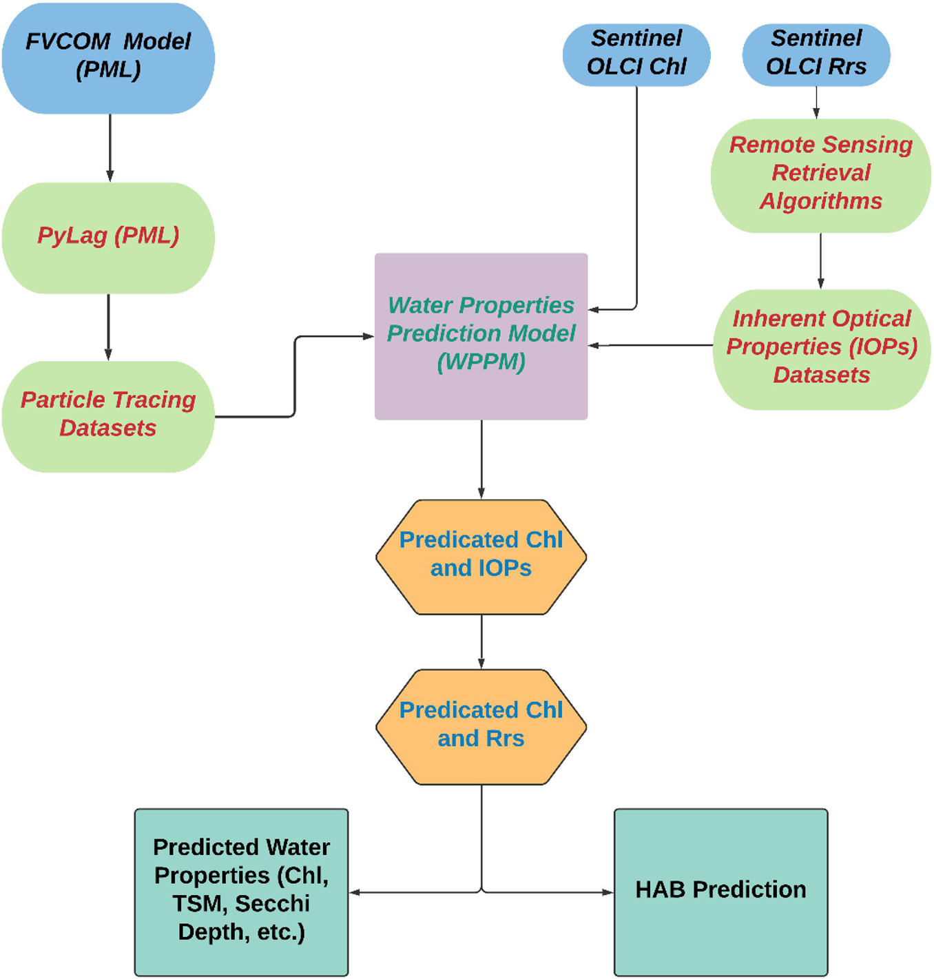
Figure 1. Flowchart of ocean color prediction algorithm for water properties and early warning maps of HAB using Lagrangian particle trajectories and ocean color observations.

where v_i is the extrapolation value of the ith pair, n is the number of extrapolations, and d is the days offset.

Prediction of Remote Sensing Reflectance

The optical spectra of water bodies provide useful information on its constituents. Hence, the above approach is revised for the capability to predict R_rs. It is worth noting that R_rs is an apparent optical property (AOP), which highly depends on the light distribution. It would be questionable if R_rs is estimated by linear weighting from extrapolations of all trajectories, as the light distribution for the particles along the trajectories could vary significantly. In this study, we propose a revised approach for prediction of R_rs based on inherent optical properties (IOPs), which solely depend on optically properties of constituents in the water but are not affected by the changes of light field. The details are described by following steps. In the first step, the quasi-analytical algorithm (QAA) is employed to retrieve IOPs: absorption (a) and backscattering (b_b) coefficients of water (Lee et al., 2002). Then a new set of IOPs is predicted from the retrieved a and b_b. Next, the predicted a and b_b are used to reconstruct R_rs with the following equation (Gordon et al., 1988).

$${\mathbf{\text{r}}}_{\mathbf{r}s}\left(\mathrm{\lambda }\right)=\left({\mathbf{\text{g}}}_{\mathbf{0}}+{\mathbf{\text{g}}}_{\mathbf{1}}\cdot \frac{{\mathbf{\text{b}}}_{\mathbf{b}}\left(\mathrm{\lambda }\right)}{\mathbf{\text{a}}\left(\mathrm{\lambda }\right)+{\mathbf{\text{b}}}_{\mathbf{b}}\left(\mathrm{\lambda }\right)}\right)\frac{{\mathbf{\text{b}}}_{\mathbf{b}}\left(\mathrm{\lambda }\right)}{\mathbf{\text{a}}\left(\mathrm{\lambda }\right)+{\mathbf{\text{b}}}_{\mathbf{b}}\left(\mathrm{\lambda }\right)}(3)$$

where g₀ = 0.0949 sr^–1, g₁ = 0.0794 sr^–1, and R_rs can be converted from r_rs with:

$${\mathbf{\text{R}}}_{\mathbf{r}s}\left(\mathrm{\lambda }\right)=\frac{0.52\cdot {\mathbf{\text{r}}}_{\mathbf{r}s}\left(\mathrm{\lambda }\right)}{\mathbf{1}-\mathbf{1.7}\cdot {\mathbf{\text{r}}}_{\mathbf{r}s}\left(\mathrm{\lambda }\right)}(4)$$

Following these steps, we are thus provided with time-series images of Chl and R_rs at 30-min intervals for the domain. These predictions are important as they will be used by algorithms to determine a quantitative estimate of HAB risk: this will be the focus of a future study. However, here we use R_rs to predict the ocean color to enable visual forecasts of bloom development.

Animation of Map Sequences

To demonstrate water property changes over time frames, we combine individual images of Chl by interpolating intermediate timesteps for a smoother appearance using the Matplotlib Animation Python package.¹ To further diagnose more details on various water types, images were composited with red–green–blue (RGB) bands from R_rs(560), R_rs(490), and R_rs(443), respectively, and animated in an analogous way. These wavelengths cover the blue–green section of the optical spectrum, within which most ocean color variability is exhibited; hence this provides an enhanced view of the ocean rather than the true color.

Results

The applicability of this prediction scheme is demonstrated by analyzing the predictions of water properties in two applications in the coastal and offshore regions of southeastern England.

The Celtic Sea and English Channel

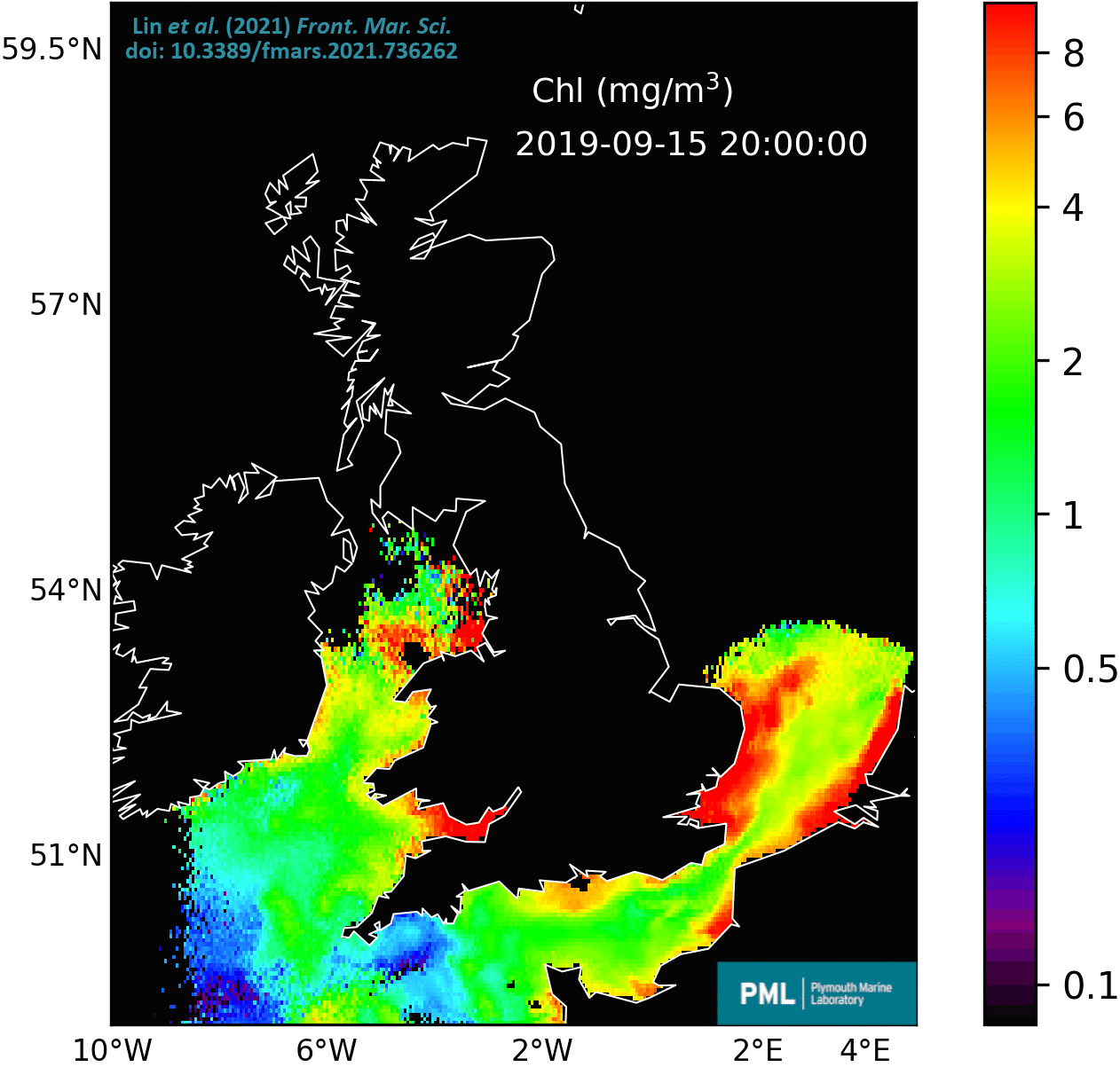
Six days of ocean color data were used for this case study (September 9–15, 2019). A total of ∼1 million particles were seeded randomly and advected at hourly intervals for 8 days from September 9 to 17, 2019, including 48 h of predictions following the satellite period, at the same spatial resolution as the ocean color data (300 m × 300 m). Figure 2 shows a map of all modeled particle trajectories over the 8 days: the path of each particle is represented by a random colored line, which overlap each other due to the high density of particles. Figure 3 shows maps of Sentinel-3 OLCI Level-3 Chl, from which we can identify the variable availability of ocean color during the 6 days due to cloud cover and orbit trajectories. There are some missing pixels in the study region but for most regions there was coverage for at least 50% of the time, e.g., for the region of English Channel, there were 3 days of ocean color observations available (September 9, 10, and 15) out of the 6 days. It is worth mentioning that from these maps we can observe that some algal blooms occurred along the coastal regions of England with high Chl (>∼4 mg/m³).

FIGURE 2

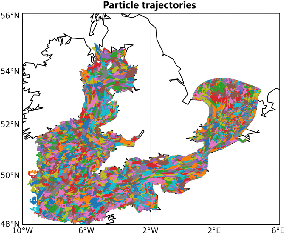
Figure 2. Particle trajectories during September 10–17, 2019, which were used for an application of the prediction scheme.

FIGURE 3

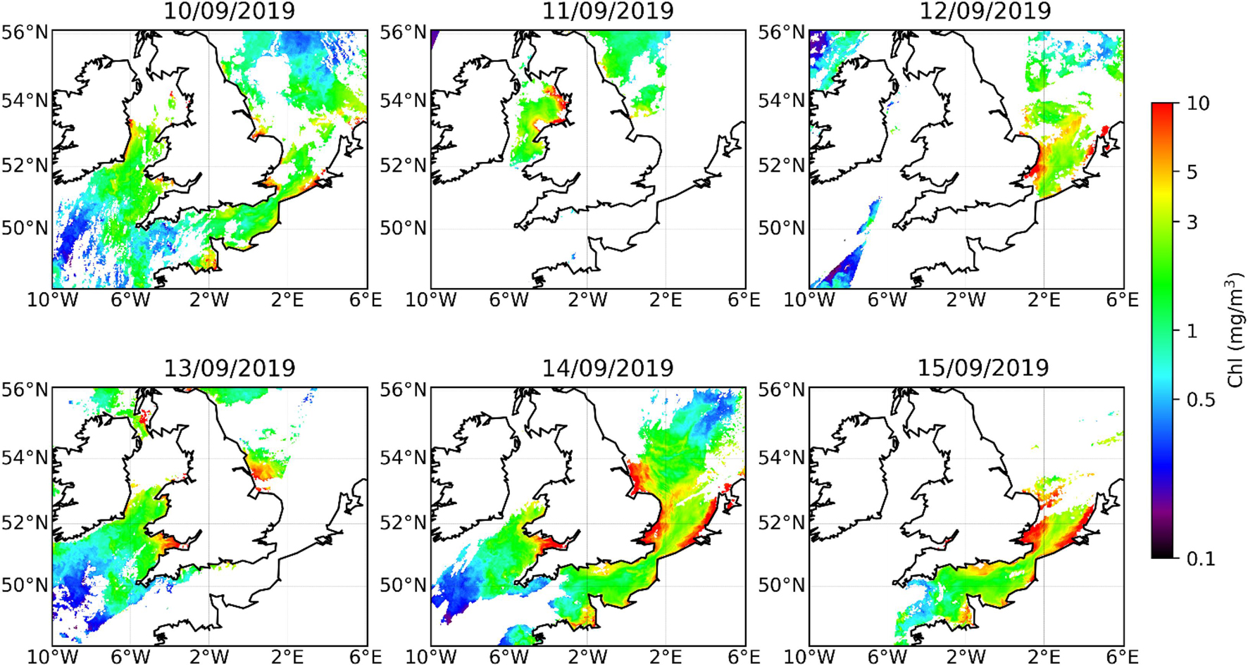
Figure 3. Maps of chlorophyll-a concentration (Sentinel-3 OLCI Level-3 products) during the days with ocean color observations used for prediction of HABs (or other bio-optical parameters).

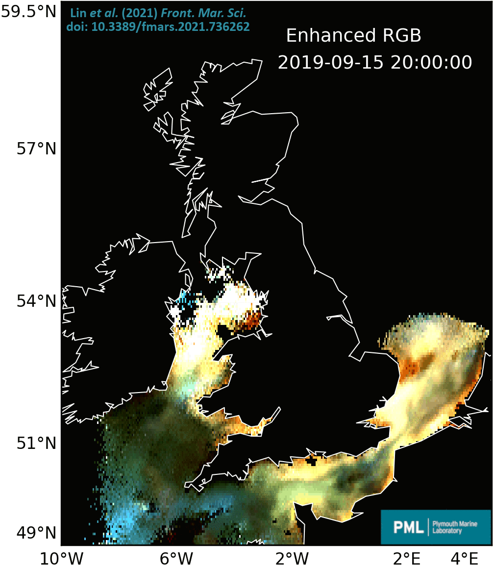
Figure 4 presents the time series predictions of Chl that shows the advection of surface waters during the first of the 2-day forecast. The most dynamic feature in this sequence is the movement of an algal bloom along the south coast of England, highlighted within the fixed ellipse in Figure 4. The value of this approach can be fully appreciated by viewing the animation of the sequence of predicted Chl maps that accompanies the figure. Advection effects are stronger in regions of the eastern English Channel with significant Chl variabilities over time, consistent with stronger tides in this region. The coastal waters generally demonstrate sharper Chl gradients than open ocean water, which is expected when considering tide, river runoff, and other forces dominating the shelf. The time series and animation of the predicted enhanced ocean-color results is shown in Figure 5: the colors in the maps indicate different water types, e.g., yellow colors in river estuaries may indicate high concentration of sediments, and dark brown colors in the eastern English Channel could be due to a suspected K. mikimotoi bloom.

FIGURE 4

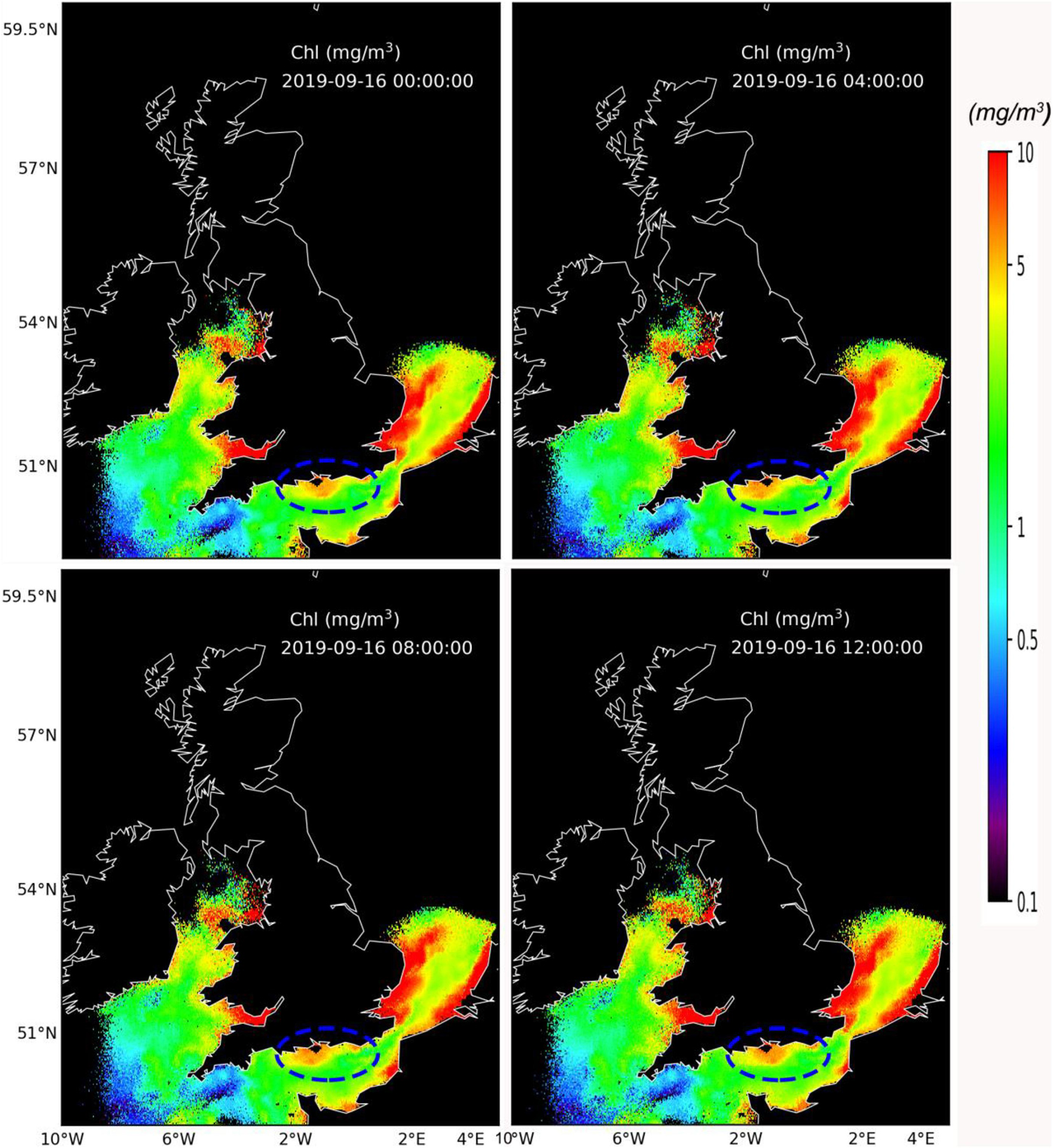
Figure 4. Frames of predicted Chl distribution at 4-h intervals during the first forecast day (September 16, 2019). The dashed ellipse is in the same location in each frame, highlighting the movement of a bloom along the south coast of England. The animation of the complete 2-day forecast can be found via https://rsg.pml.ac.uk/shared_files/junl/paper_animation/example1/chl.gif.

FIGURE 5

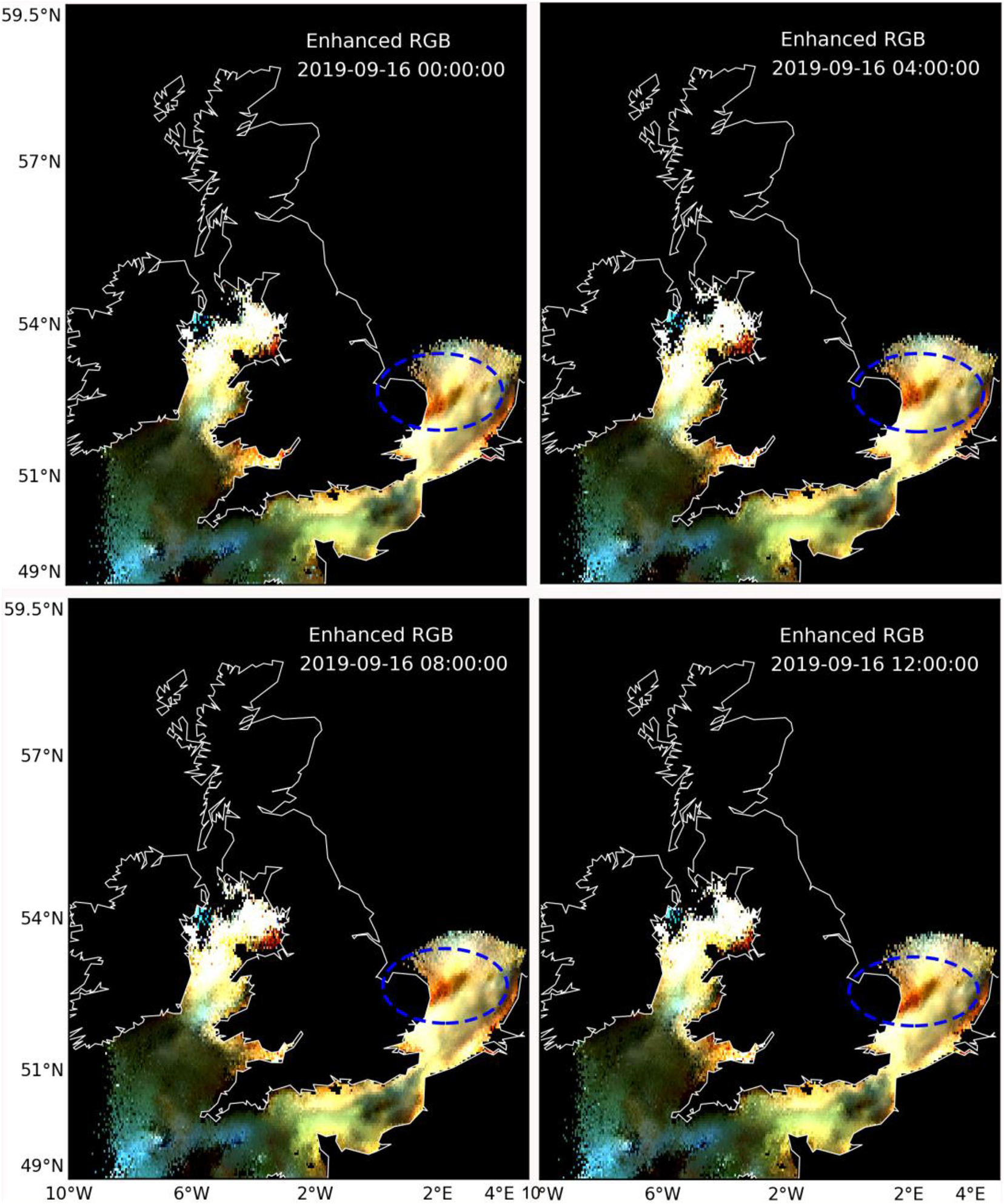
Figure 5. Frames of predicted enhanced ocean-color RGB images indicating variabilities of water types (animation: https://rsg.pml.ac.uk/shared_files/junl/paper_animation/example1/rgb.gif).

To further demonstrate the efficiency of the prediction approach, the conditions of water quality were also studied by plotting changes over time. Three transects were selected along latitudes 50° N, 51.3° N, and 52.5° N (Figure 6), covering possible bloom regions (e.g., estuaries, south-east England coasts). Figure 7 shows the time series and animation of predicted Chl along the three transects. It was found that Chl varied over a wide range each day, usually with a periodic pattern mainly due to different stages of the tidal cycle that influence the advection of water parcels. In Figure 7B, the upward slope indicates a net westward advection of water along the transect.

FIGURE 6

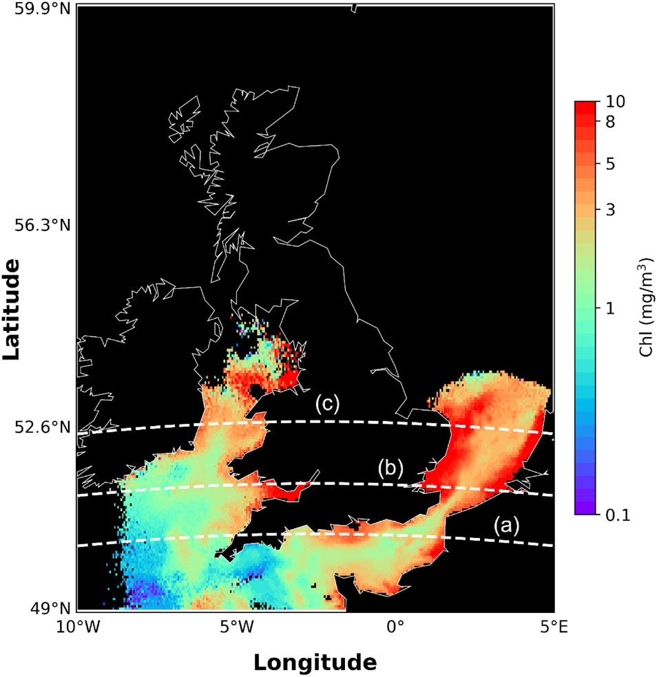
Figure 6. Map showing the distribution of predicted Chl at 15th September 8 p.m. (first predicted image) overlaid with lines of latitudes at 50° N, 51.3° N, and 52.5° N.

FIGURE 7

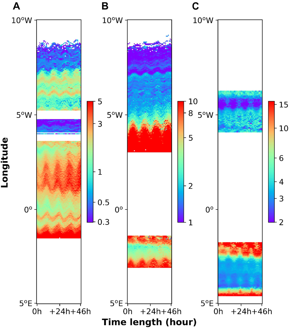
Figure 7. Hovmöller plot showing time series of predicted Chl (mg/m³) along zonal lines: (A) 50° N, (B) 51.3° N, and (C) 52.5° N.

An error estimation for the prediction algorithm was performed by comparing the predicted Chl on the second forecast day (September 17, 2019 12:00 p.m.) against the satellite-observed Chl scene that day (12:29 p.m.). The scatter plot of cloud-free pixels in the two datasets are shown in Figure 8. The predicted Chl agrees well with satellite Chl with an r² of 0.81 and a mean absolute percentage error (MAPE) of 36.9%. The MAPE is defined by

$$MAPE=\frac{1}{n}\sum _{i=1}^n\left|\frac{x_p-x_s}{x_s}\right|(5)$$

FIGURE 8

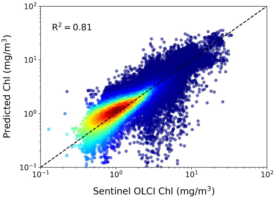
Figure 8. Comparison of Sentinel OLCI Chl with predicted Chl on September 17, 2019 (MAPE = 36.9%); the linear regression between the two datasets is y = 0.79 x + 0.28 (r² = 0.81).

with x_p and x_s representing predicted and satellite values, respectively, n is the number of values. The results further demonstrate the robust performance of the prediction scheme for changes of water properties.

High Spatial Resolution in English Channel

Monitoring of water bodies at high spatial resolution is of paramount importance, especially in dynamic coastal waters, where the water constituents can vary dramatically over a small distance. To evaluate the ability of the prediction algorithm for high spatial resolution, a further period was studied in the English Channel, June 29 to July 5, 2019 when a large coccolithophore bloom was observed. In this case, many more particles were seeded (∼10 million particles). To demonstrate the techniques using computer time feasible for an operational monitoring system, the region of interest was limited to the English Channel and only 16 h of predictions were generated. The spatial resolution of the resulting prediction images is 100 m with a temporal resolution of 1 h. Figure 9 shows and animates the changes of Chl distributions over time. Small scale structures are interpreted here (e.g., some fine structures of algae patches were revealed). To gain a precise understanding of water types, the enhanced ocean-color images with high spatial resolution are shown and animated in Figure 10. The (harmless) coccolithophorid bloom occurred in the northern English Channel, covering thousands of square kilometers with milky blue. The prediction method here successfully discriminated the locations of the bloom and its advection over time, further demonstrating the value of using this prediction method for monitoring algal blooms.

FIGURE 9

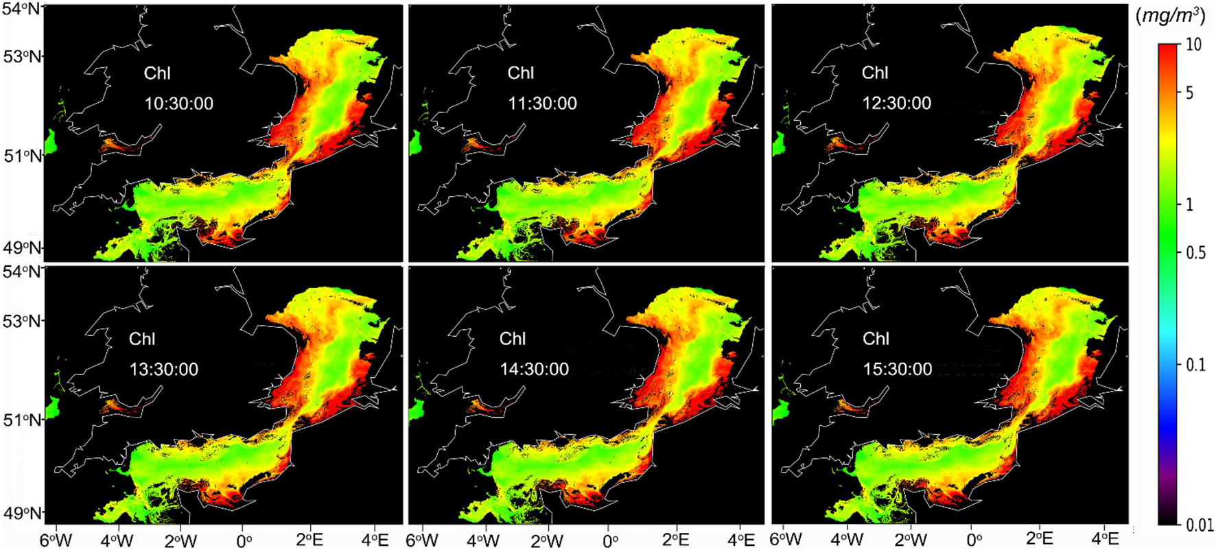
Figure 9. Prediction algorithm applied to the English Channel, June 29 to July 5, 2019: maps showing distribution of predicted Chl at 4-h intervals with high spatial resolution (100 m) (animation: https://rsg.pml.ac.uk/shared_files/junl/paper_animation/example2/chl.gif).

FIGURE 10

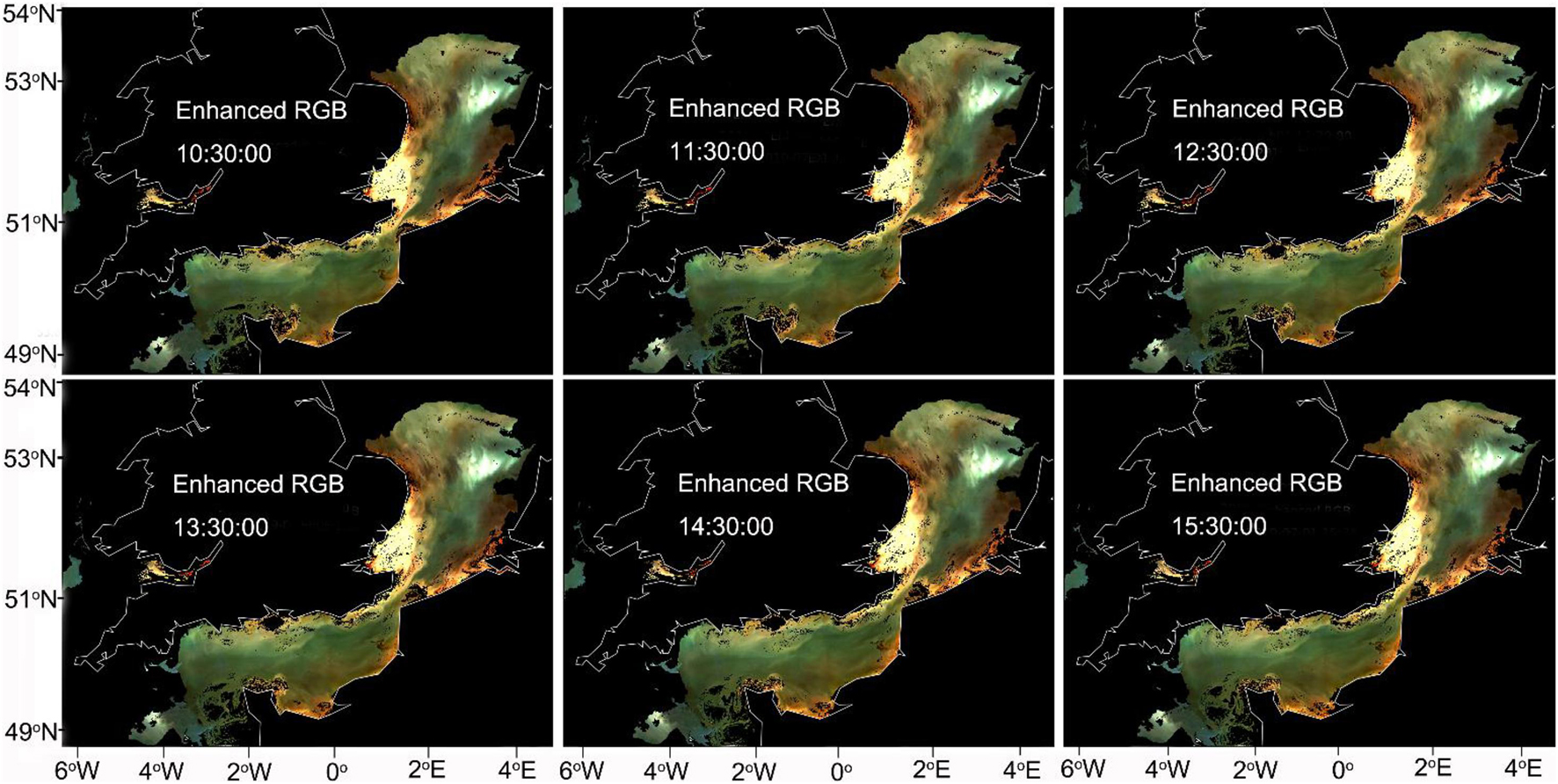
Figure 10. Frames of predicted enhanced ocean-color RGB in the English Channel with high spatial resolution (100 m) showing more details of water properties including the movement of a bright coccolithophore bloom near 53° N (animation: https://rsg.pml.ac.uk/shared_files/junl/paper_animation/example2/rgb.gif).

Discussion

It is quite clear, as seen both in our findings and in earlier studies (e.g., Jönsson et al., 2009; Jönsson and Salisbury, 2016), that biological processes in coastal are strongly affected by physical advection of water parcels, and that combining satellite derived products and simulated velocity fields using particle tracking provides a powerful approach for such analyses. While earlier works by Jönsson et al. (2011) and Jönsson and Salisbury (2016) are primarily focused on estimating the rate of change in satellite properties, we present results showing that the method can be expanded to predict locations and concentrations of the properties. This novel application can be used to better predict HAB events and to identify the extent and location of blooms more precisely, especially in regions with strong tidal cycles where surface currents are predictable.

We find our results to be generally physically coherent and that any patches of high phytoplankton biomass are predicted and advected in a reasonable way. The nature of the method is such that we expect significant methodological errors to be seen as noise or spurious changes in our predicted fields (see Jönsson et al., 2009 for further discussion). We see for example, as expected, generally sharper Chl gradients in coastal waters compared to the open ocean in the Celtic Sea and English Channel. The method is also able to successfully predict the location of a coccolithophore bloom. The skill of the method discussed here is in line with what earlier studies have reported from the California Current (Jönsson and Salisbury, 2016) and Gulf of Maine (Jönsson et al., 2009) when estimating rates of change, which suggests that the extrapolation approach has a similar ability to provide useful information.

While the prediction tool presented in this study has the potential to improve regional HAB monitoring by more precisely assessing how the current state will develop in the near future, we readily agree that there are limitations. It is inevitable that there will be inaccuracies due to imperfections in the modeling and methodology. Errors in the prediction method could arise from many aspects, e.g., imperfect velocity of fields, extrapolation of model velocities in time and space, numerical integration of the trajectory path, and the omission of vertical velocity.

In this study, Lagrangian particle trajectories were computed according to the effect of both advection and diffusion. However, because each trajectory only contains a limited number of particles, the final locations of simulated particles could not be representative of all possible particle locations due to diffusion. The problem could be especially acute for some areas with large horizontal current shear. Thus, it would be important to keep in mind that uncertainty from diffusion always exists in these areas. The problems could be solved by seeding many more particles at each initial location, though the additional burden of computing their trajectories is currently unfeasible for this real-time application. A practical solution could be to introduce a probability density function indicating possible locations for each traced particle. However, it is beyond the scope of this study and substantial studies of this question are anticipated in the future. Regarding errors from advection, this was assessed in the previous study of Jönsson et al. (2009) by comparing the changes in Chl and sea surface temperature (SST) between the start and end positions of particle trajectories advected between two satellite images. The results showed that the advective errors are small relative to total changes due to other factors.

The extrapolation procedure will also introduce errors to the predictions. The predicted values were estimated via linear extrapolation with a weighting function. To reduce error from the extrapolation, when the extrapolated value for a trajectory exceeded 50% of the mean value of all extrapolations, this trajectory was disregarded and was not included for the calculation of final prediction. Considering uncertainty from the IOPs retrieval algorithm, errors in predicted IOPs are inevitable, but errors in R_rs could possibly be compensated by reconstruction from these IOPs. Furthermore, it is also worth noting that although individual trajectories have errors, the statistics obtained from thousands of particles are still very informative.

Still, while not perfect, the resulting predictions provide an enhanced set of information for managers and stakeholders to include when assessing the risk of HABs that has not been available until now. The prediction tool is also agnostic to any of its component modules. We are able to easily leverage new improved ocean circulation models and satellite products into the framework to provide as accurate predictions as possible.

Conclusion

This study set out to develop a prediction scheme for monitoring HABs by merging satellite observations and Lagrangian particle tracking. Two case studies in regions along the coast of England have shown that the Lagrangian methodology is effective for the interpretation of satellite data for early warning of HAB risk. The accuracy of the predictions relies on many factors. Particularly, the uncertainties from modeling and methodology, e.g., velocity of fields, extrapolation of model velocities in time and space, numerical integration of the trajectory path, and the omission of vertical velocity, may have big impacts on determining the accuracy of final predictions. Notwithstanding these imperfections, this work offers a powerful tool for monitoring and observing the state of the marine ecosystem. The synoptic, time-resolved quantification is invaluable to our understanding of HABs developments. Animated sequences generated by this method promote greater understanding and usage of satellite ocean color data for communicating with aquaculture farmers. Future research will extend the approach to predict quantitative risk maps for key high-biomass HAB species. Hence our future priority is to seek further applications of this new technique to support the aquaculture industry with improved early warning of potential HABs.

Data Availability Statement

The raw data supporting the conclusions of this article will be made available by the authors, without undue reservation.

Author Contributions

JL developed the prediction scheme, implemented the code, and wrote the first draft of the manuscript. PM proposed initial ideas and helped shape the research. BJ provided suggestions on code and algorithm development. MB helped carry out numerical simulations. All authors discussed the results and commented on the manuscript.

Funding

This study was supported by the Interreg Atlantic Area Programme project “Predicting the Impact of Regional Scale Events on the Aquaculture Sector” (PRIMROSE, Grant No. EAPA_182/2016) and UK BBSRC project “Safe and Sustainable Shellfish: Introducing local testing and management solutions” (reference BB/S004211/1). BJ was in part funded by NASA 80NSSC21K0565 and a Simons Foundation grant (549947, SS).

Conflict of Interest

The authors declare that the research was conducted in the absence of any commercial or financial relationships that could be construed as a potential conflict of interest.

Publisher’s Note

All claims expressed in this article are solely those of the authors and do not necessarily represent those of their affiliated organizations, or those of the publisher, the editors and the reviewers. Any product that may be evaluated in this article, or claim that may be made by its manufacturer, is not guaranteed or endorsed by the publisher.

Footnotes

1. ^ https://imageio.github.io

References

Anderson, D. M. (2009). Approaches to monitoring, control and management of harmful algal blooms (HABs). Ocean Coastal Manage. 52, 342–347. doi: 10.1016/j.ocecoaman.2009.04.006

PubMed Abstract | CrossRef Full Text | Google Scholar

Anderson, D. M., Cembella, A. D., and Hallegraeff, G. M. (2012). Progress in understanding harmful algal blooms: paradigm shifts and new technologies for research, monitoring, and management. Annu. Rev. Mari. Sci. 4, 143–176. doi: 10.1146/annurev-marine-120308-081121

PubMed Abstract | CrossRef Full Text | Google Scholar

Anderson, D. M., Hoagland, P., Kaoru, Y., and White, A. W. (2000). Estimated Annual Economic Impacts From Harmful Algal Blooms (HABs) in the United States. Woods Hole, MA: WHOI-2000-11Woods Hole Oceanogr Inst.

Google Scholar

Blondeau-Patissier, D., Gower, J. F., Dekker, A. G., Phinn, S. R., and Brando, V. E. (2014). A review of ocean color remote sensing methods and statistical techniques for the detection, mapping and analysis of phytoplankton blooms in coastal and open oceans. Prog. Oceanogr. 123, 123–144. doi: 10.1016/j.pocean.2013.12.008

CrossRef Full Text | Google Scholar

Chen, C., Liu, H., and Beardsley, R. C. (2003). An unstructured grid, finite-volume, three-dimensional, primitive equations ocean model: application to coastal ocean and estuaries. J. Atmospheric Terrest. Phys. 20, 159–186. doi: 10.1175/1520-0426(2003)020<0159:augfvt>2.0.co;2

CrossRef Full Text | Google Scholar

Fernandes-Salvador, J. A., Davidson, K., Sourisseau, M., Revilla, M., Schmidt, W., Clarke, D., et al. (2021). Current status of forecasting toxic harmful algae for the north-east Atlantic shellfish aquaculture industry. Front. Mari. Sci. 8:666583.

Google Scholar

Fogg, G. E. (1969). The physiology of an algal nuisance. Proc. R. Soc. London Seri. B 173, 175–189. doi: 10.1098/rspb.1969.0045

CrossRef Full Text | Google Scholar

Gobler, C. J. (2020). Climate change and harmful algal blooms: insights and perspective. Harmful Algae 91:101731. doi: 10.1016/j.hal.2019.101731

PubMed Abstract | CrossRef Full Text | Google Scholar

Gordon, H. R., Brown, O. B., Evans, R. H., Brown, J. W., Smith, R. C., Baker, K. S., et al. (1988). A semianalytic radiance model of ocean color. J. Geophy. Res. Atmosph. 93, 10909–10924. doi: 10.1029/jd093id09p10909

CrossRef Full Text | Google Scholar

Grattan, L. M., Holobaugh, S., and Morris, J. G. Jr. (2016). Harmful algal blooms and public health. Harmful Algae 57, 2–8. doi: 10.1016/j.hal.2016.05.003

CrossRef Full Text | Google Scholar

Hallegraeff, G. (2003). Harmful algal blooms: a global overview. Manual Harmful Mari. Microalgae 33, 1–22. doi: 10.1007/978-0-387-75865-7_1

CrossRef Full Text | Google Scholar

Hallegraeff, G. M. (1993). A review of harmful algal blooms and their apparent global increase. Phycologia 32, 79–99. doi: 10.1186/1476-069X-7-S2-S4

PubMed Abstract | CrossRef Full Text | Google Scholar

Heisler, J., Glibert, P. M., Burkholder, J. M., Anderson, D. M., Cochlan, W., Dennison, W. C., et al. (2008). Eutrophication and harmful algal blooms: a scientific consensus. Harmful Algae 8, 3–13. doi: 10.1016/j.hal.2008.08.006

PubMed Abstract | CrossRef Full Text | Google Scholar

Jönsson, B. F., and Salisbury, J. E. (2016). Episodicity in phytoplankton dynamics in a coastal region. Geophy. Res. Lett. 43, 5821–5828. doi: 10.1002/2016gl068683

CrossRef Full Text | Google Scholar

Jönsson, B. F., Salisbury, J. E., and Mahadevan, A. J. I. (2009). Extending the use and interpretation of ocean satellite data using Lagrangian modelling. Int. J. Remote Sen. 30, 3331–3341. doi: 10.1080/01431160802558758

CrossRef Full Text | Google Scholar

Jönsson, B., Salisbury, J., and Mahadevan, A. (2011). Large variability in continental shelf production of phytoplankton carbon revealed by satellite. Biogeosciences 8:1213. doi: 10.5194/bg-8-1213-2011

CrossRef Full Text | Google Scholar

Klemas, V. J. (2012). Remote sensing of algal blooms: an overview with case studies. J. Coas. Res. 28, 34–43. doi: 10.2112/jcoastres-d-11-00051.1

CrossRef Full Text | Google Scholar

Kwon, K., Choi, B.-J., Kim, K. Y., and Kim, K. (2019). Tracing the trajectory of pelagic sargassum using satellite monitoring and Lagrangian transport simulations in the East China sea and yellow sea. Algae 34, 315–326. doi: 10.4490/algae.2019.34.12.11

CrossRef Full Text | Google Scholar

Landsberg, J. H. (2002). The effects of harmful algal blooms on aquatic organisms. Rev. Fish. Science 10, 113–390. doi: 10.1080/20026491051695

CrossRef Full Text | Google Scholar

Lee, Z., Carder, K. L., and Arnone, R. A. (2002). Deriving inherent optical properties from water color: a multiband quasi-analytical algorithm for optically deep waters. Appl. Optics 41, 5755–5772. doi: 10.1364/ao.41.005755

PubMed Abstract | CrossRef Full Text | Google Scholar

Li, H., Qin, C., He, W., Sun, F., and Du, P. (2020). Prototyping a numerical model coupled with remote sensing for tracking harmful algal blooms in shallow lakes. Global Ecol. Conserv. 22:e00938. doi: 10.1016/j.gecco.2020.e00938

CrossRef Full Text | Google Scholar

Mueller, J. (1981). Prospects for Measuring Phytoplankton Bloom Extent and Patchiness Using Remotely Sensed Color Images. New York: Toxic Dinoflagellate Blooms, Elsevier, North Holland, Inc., 303–330.

Google Scholar

Olascoaga, M. J., Beron-Vera, F. J., Brand, L. E., and Koçak, H. J. (2008). Tracing the early development of harmful algal blooms on the west Florida shelf with the aid of lagrangian coherent structures. J. Geophys. Res. Oceans 113:c12014. doi: 10.1029/2007JC004533

PubMed Abstract | CrossRef Full Text | Google Scholar

Paerl, H. W. (1988). Nuisance phytoplankton blooms in coastal, estuarine, and inland waters 1. Limnol. Oceanogr. 33, 823–843. doi: 10.4319/lo.1988.33.4_part_2.0823

CrossRef Full Text | Google Scholar

Sellner, K. G., Doucette, G. J., and Kirkpatrick, G. J. (2003). Harmful algal blooms: causes, impacts and detection. J. Indust. Microbiol. 30, 383–406. doi: 10.1007/s10295-003-0074-9

PubMed Abstract | CrossRef Full Text | Google Scholar

Sengco, M. R., and Anderson, D. M. (2004). Controlling harmful algal blooms through clay flocculation 1. J. Eukaryotic Microbiol. 51, 169–172. doi: 10.1111/j.1550-7408.2004.tb00541.x

PubMed Abstract | CrossRef Full Text | Google Scholar

Smagorinsky, J. (1963). General circulation experiments with the primitive equations: I. the basic experiment. Monthly Weather Rev. 91, 99–164. doi: 10.1175/1520-0493(1963)091<0099:gcewtp>2.3.co;2

CrossRef Full Text | Google Scholar

Son, Y. B., Choi, B.-J., Kim, Y. H., and Park, Y. G. (2015). Tracing floating green algae blooms in the Yellow sea and the East China sea using GOCI satellite data and lagrangian transport simulations. Remote Sensing Environ. 156, 21–33. doi: 10.1016/j.rse.2014.09.024

CrossRef Full Text | Google Scholar

Tilstone, G. H., Pardo, S., Dall’Olmo, G., Brewin, R. J. W., Nencioli, F., Dessailly, D., et al. (2020). Performance of ocean colour chlorophyll a algorithms for sentinel-3 1 OLCI, MODIS-aqua and suomi-VIIRS in open-ocean waters of the Atlantic. Remote Sens. Environ. 260:art.112444. doi: 10.1016/j.rse.2021.112444

CrossRef Full Text | Google Scholar

Umlauf, L., and Burchard, H. (2005). Second-order turbulence closure models for geophysical boundary layers. a review of recent work. Continental Shelf Res. 25, 795–827. doi: 10.1016/j.csr.2004.08.004

CrossRef Full Text | Google Scholar

Uncles, R., Clark, J. R., Bedington, M., and Torres, R. (2019). Physical Processesl in the Whitsand Bay Marine Conservation Zone: Neighbour to a Closed Dredge-Spoil Disposal Site. Amsterdam: Marine Protected Areas, Elsevier.

Google Scholar

Wynne, T. T., Stumpf, R. P., Tomlinson, M. C., Schwab, D. J., Watabayashi, G. Y., and Christensen, J. D. (2011). Estimating cyanobacterial bloom transport by coupling remotely sensed imagery and a hydrodynamic model. Ecol. Appl. 21, 2709–2721. doi: 10.1890/10-1454.1

CrossRef Full Text | Google Scholar