Uncertainty in Atlantic Multidecadal Oscillation derived from different observed datasets and their possible causes

Introduction

The Atlantic Multidecadal Oscillation (AMO) is a leading mode of multi-decadal variability that produces a basin-wide warming/cooling in the North Atlantic (Schlesinger and Ramankutty, 1994) with high spatial coherence (hereafter referred to as the “coherent AMO pattern”). Both observational and modeling studies show that the influence of the AMO on climate is not limited to the Atlantic area, but operates on a global scale, such as its role in Atlantic hurricanes (Goldenberg et al., 2001; Zhang and Delworth, 2006; Enfield and Cid-Serrano, 2009), temperature and rainfall over land (Sutton and Hodson, 2005; Knight et al., 2006; Tao et al., 2021), and the rate of global warming (DelSole et al., 2011; Chen and Tung, 2017).

Although the coherent AMO pattern has been regarded as a key physical feature of the AMO (Zhang et al., 2019) and widely used to distinguish its driving mechanism (Sun et al., 2018), it is still spatially heterogeneous, with higher anomalies in the subpolar and tropical North Atlantic and lower anomalies in the subtropical region, referred to as a “horseshoe-like” pattern. Previous studies have indicated that this horseshoe-like SST pattern is mainly associated with the North Atlantic Oscillation in slab ocean models (Clement et al., 2015; Sun et al., 2015), and that dynamic processes related to the Atlantic Meridional Overturning Circulation (AMOC) play a critical role in the coherent AMO pattern in coupled models via altering oceanic meridional heat transport (Knight et al., 2005; Zhang, 2008; Sun et al., 2020a). This AMOC-related meridional heat transport contributes mainly to the coherent AMO pattern in the extratropics (Sun et al., 2020b). The connection between the tropical part of the AMO and its subtropical and subpolar parts may primarily occur via rapid atmospheric processes such as those related to aerosols and cloud (Booth et al., 2012; Brown et al., 2016; Zhang et al., 2019). Nevertheless, the subtropical part of the AMO contains large observational uncertainty, as reported by IPCC AR6 (Eyring et al., 2021). Therefore, it is necessary to examine how coherent the observed AMO pattern is, and to detect where the uncertainties of the AMO pattern arise in observational datasets.

Multiple lines of evidence show a typical periodicity of 50–80 years for the observed AMO (Schlesinger and Ramankutty, 1994; Gray et al., 2004). This long periodicity and the coexistence of both AMO and global warming signals in observed SST data poses significant challenges to studying the AMO observationally. To avoid possible spurious results and disentangle the effects of global warming and the AMO on regional and global climate, an observational record of at least 80 years is required (Tung and Zhou, 2013; Frankignoul et al., 2017; Wills et al., 2019). Although climate models can provide sufficiently long records to resolve multiple AMO cycles, simulations of the AMO suffer from both shorter periodicities (typically 10–30 years) and much weaker amplitudes than observation (Ruiz-Barradas et al., 2013; Zhang and Wang, 2013). This incapability of most models to reproduce the dominant observed AMO periodicity (50–80 years) hinders the extent to which the AMO can be studied (Lin et al., 2019). Therefore, sufficiently long historical observations and/or reconstructions (>80 years) of SST data still provide the best opportunities to study the observed AMO.

Several century-long global gridded SST datasets are widely used to study the AMO, such as the Extended Reconstructed SST dataset version 5 (ERSSTv5, Huang et al., 2017), the Hadley Centre Sea Ice and Sea Surface Temperature dataset (HadISSTv1.1, Rayner et al., 2003), and the Centennial In Situ Observation-Based Estimates of the Variability of SST and Marine Meteorological Variables version 2 (COBE-SST2, Hirahara et al., 2014). Although common AMO features are recognized based on these datasets, such as the strongest signal being located over the subpolar North Atlantic and the relatively weaker signal over the tropics, they are not completely identical across different observational datasets (Frankignoul et al., 2017; Eyring et al., 2021). Although studies have suggested that SST differences can be induced by the different bias-adjustment schemes in different SST datasets because they may lead to different SST decadal variation (Huang et al., 2015; Kent et al., 2017), almost no attention has been paid to the connections between these SST differences and the resulting AMO using different observational datasets.

The aim of this study is to discover the uncertainties of the resulting AMO time series and its spatial patterns derived from different datasets and to explore the possible causes of these uncertainties. To achieve this, the AMO signal is extracted from three different observational SST datasets (ERSSTv5, HadISSTv1.1 and COBE-SST2) for the period 1900–2019 by using an objective method that does not presume in advance the existence of SST trends due to global warming—namely, Low-Frequency Component Analysis (LFCA, Wills et al., 2019). The LFCA can extract the spatially uneven trend. We also explore the differences between different versions of the same dataset to see if the same AMO biases are inherited from one generation of the dataset to the next. The first part shows the discrepancy of AMO from various datasets, the second and third part are the temporal period and regions in which data impacted the AMO. The fourth and fifth part investigate the technique and seasonal correction that contribute to the discrepancy of AMO. Finally, the role of data uncertainty and detrending method in AMO are examined.

Results

The AMO from various datasets

Figures 1A, C and E show the AMO patterns extracted from the North Atlantic (0°–65°N) SST in three monthly observational datasets [ERSSTv5 (ERv5), HadISSTv1.1 (HadI1) and COBE-SST2 (COBE2)], for 1900–2019, using LFCA. A horseshoe-like AMO pattern appears in all datasets, with the maximum anomaly in the subpolar North Atlantic and a weaker one in the tropics, which is a spatial structure in agreement with previous studies (Zhang et al., 2019) and the CMIP6 multi-model ensemble mean (Eyring et al., 2021). However, the spatial coherence of the AMO pattern in the Atlantic is quite different in these three datasets. To quantify the spatial coherence, we define a coherence index (CI), which represents the percentage of grid points with anomalies that have the same positive sign, for which we empirically determined that if the CI is greater than 89%, the AMO pattern is spatially coherent; otherwise, it is not (see DATA AND METHOD). The CI is over 93% for HadI1 and COBE2, but only 69.2% for ERv5. Thus, the AMO spatial pattern is coherent if it is derived from HadI1 or COBE2, but not if it is derived from ERv5. There are negative anomalies in a significant portion of the subtropical and equatorial North Atlantic for ERv5, which do not appear in the traditionally defined AMO pattern (Trenberth and Shea, 2006) or in the HadI1 and COBE2 datasets. The pattern correlation coefficient (PCC) between the AMO derived from ERv5 and that derived from HadI1/COBE2 is only 0.53/0.73 (Table 1), which is much lower than the AMO PCC between HadI1 and COBE2 (0.86). By considering both the CI and pattern correlations, we conclude that the AMO spatial pattern derived from ERv5 is significantly different from that derived from either of the other two datasets.

FIGURE 1

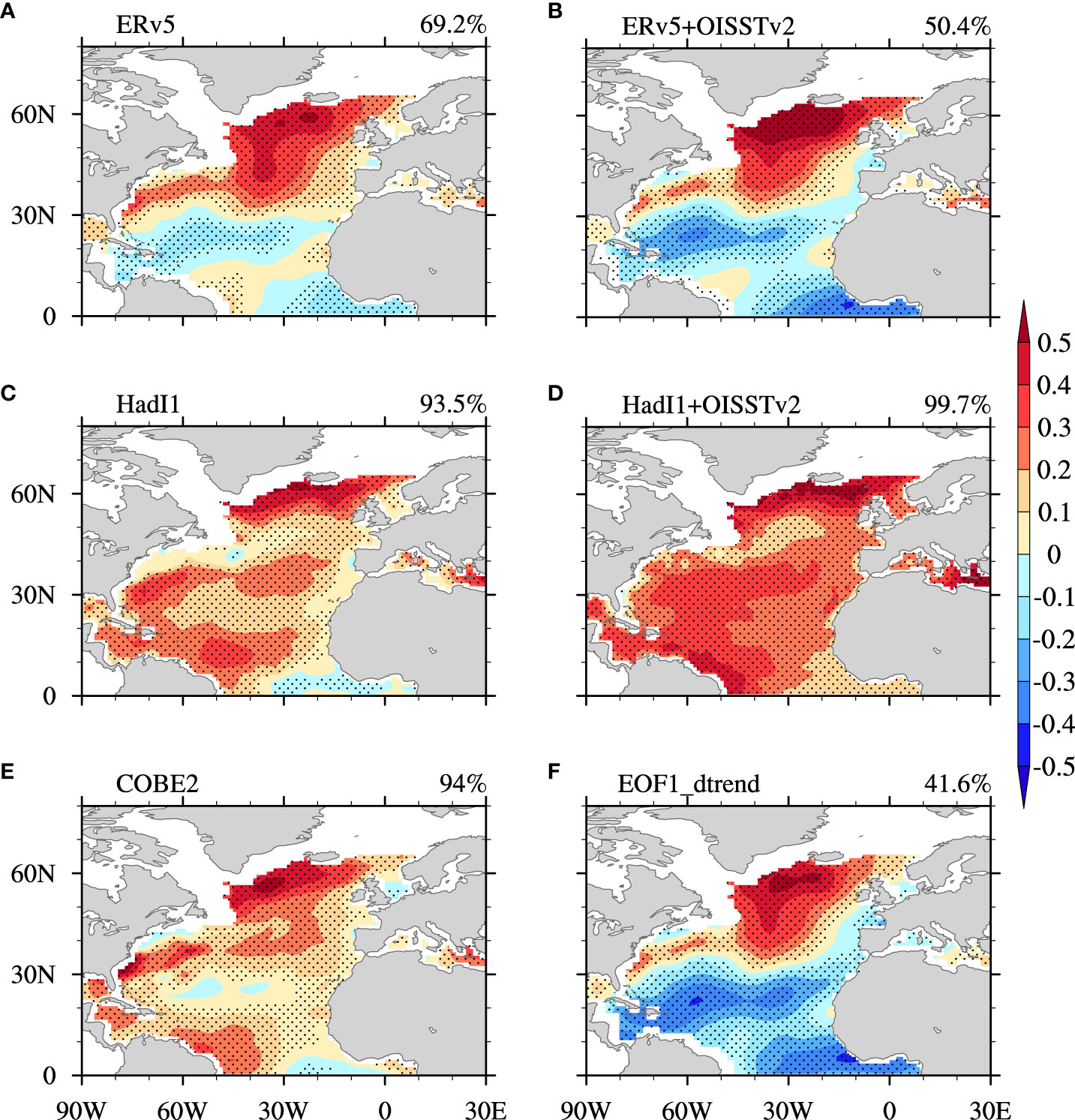
Figure 1 Spatial pattern of the AMO extracted by LFCA from different SST datasets over the period 1900–2019: (A, C, E) ERv5, HadI1, and COBE2, respectively. (B) ERv5 in 1900–1981 and OISSTv2 in 1982–2019. (D) HadI1 in 1900–1981 and OISSTv2 in 1982–2019. (F) Leading mode of LFCA after removing the first leading EOF mode and the principal component (i.e., the inhomogeneous warming trend) over the North Atlantic. The second/third leading low-frequency pattern and component of monthly SSTA in ERv5(COBE2)/HadI1 is the AMO pattern and index, respectively. The AMO CI from each dataset is denoted in the top-right corner of the figure. Dots indicate the value passes the 95% significance level. Unit: °C.

TABLE 1

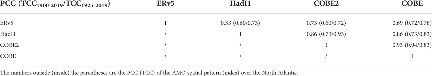
Table 1 The PCCs and TCCs of AMO indices and spatial patterns over the North Atlantic. A 10-year low-pass filter is applied to obtain AMO indices derived from four SST datasets.

To further identify this low CI in AMO pattern (hereafter referred to as incoherent AMO pattern) in ERv5, we swap the SST data between 1982 and 2019 in each dataset with those from version 2 of the Optimum Interpolation Sea Surface Temperature dataset (OISSTv2, Reynolds et al., 2007) and keep the SST data unchanged for the period 1900–1981, similar to the study of Si et al. (2020). Note that we also tested to use different years around 1981 to split the datasets and our results are insensitive to the exact splitting year (not shown). After applying LFCA to the merged SSTs, the resulting AMO patterns for “merged-HadI1” (Figure 1D) and “merged-COBE2” (figure not shown) are almost unchanged with a slightly higher spatial coherence (CI = 99.7% vs. 93.5%). In contrast, the AMO pattern derived from “merged-ERv5” shows an even lower spatial coherence (50.4% vs. 69.2%; Figure 1B). This result confirms that the low spatial coherence of the AMO pattern in ERv5 is not due to the use of LFCA, and the cause for this low coherence is related to the ERv5 data in the period 1900–1981, especially the data in the subtropical to equatorial North Atlantic.

Next, we explore the similarity in the AMO’s temporal evolution. The second low-frequency components/patterns in the ERv5 and COBE2 datasets are AMO indexes/patterns and their first leading components/patterns are the North Atlantic warming trend time series/patterns (Figures 1, 2A, D). Whereas in HadI1, the first two leading LFCA time series/patterns are the North Atlantic warming trend time series/patterns and the third mode is the AMO indexes/pattern (Figures 1, 2A, D), similar to the result in Wills et al. (2019). Generally, the AMO index (Figure 2A) varies similarly, with temporal correlation coefficients (TCCs) greater than 0.6 (Table 1) across the different datasets with three dominant phase transitions around the years 1920, 1970 and 2000 during 1900–2019. However, the AMO phase transitions in ERv5 precede those in the other two datasets by 10–15 years (Figure 2B), particularly during the period 1930–1970. This is reflected by the lower TCCs between the AMO indices derived from ERv5 and from HadI1/COBE2 than between the AMO indices derived from HadI1 and COBE2 (0.6 vs. 0.73 for the period 1900–2019, or ~0.72 vs. 0.93 for the period 1925–2019; Table 1). It is worth highlighting that the peaks of the AMO index during 1930–1950 are higher in ERv5 than in HadI1 and COBE2, which is in agreement with the result reported in chapter 3 of IPCC AR6 (Eyring et al., 2021). Therefore, we conclude that it is not only the spatial pattern of the AMO derived from ERv5 that differs from its counterparts in the other two datasets, but also the AMO index. These differences arise mainly from the subtropical to tropical Atlantic SSTs, and from the SST data before 1981 as explored in the next two subsections.

FIGURE 2

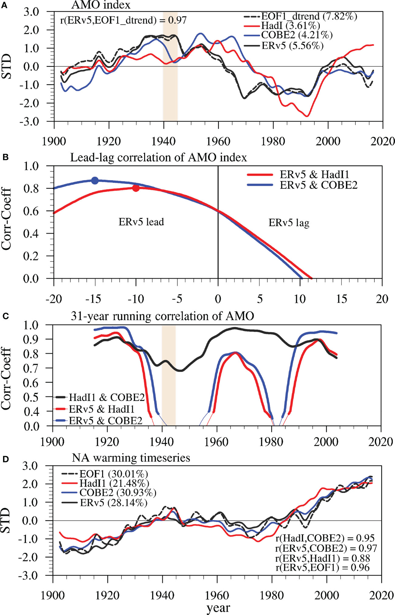
Figure 2 (A) AMO index extracted by LFCA from ERv5, COBE2 and HadI1, in which the dashed line is the AMO index extracted by LFCA after removing the first EOF mode and principal component of NASST in ERv5. (B) Lead–lag correlation coefficients between the AMO index in ERv5 and those in HadI1 (blue) and COBE2 (red) in 1900–2019, in which the dots represent the positions with the maximal correlation coefficients. (C) 31-year running correlation of AMO indices among different datasets, in which the thick (thin) lines denote values passing (failing) the 99% significance level. (D) The warming trend time series in the North Atlantic (the first low-frequency component of LFCA) from ERv5, COBE2 and HadI1, in which the dashed line is the first principal component from EOF in ERv5. The explained variances (%) and TCCs are shown.

The critical period leading to the uncertainty in reproducing the coherent pattern of AMO

To identify the periods in which the AMO index derived from ERv5 differs from those derived from HadI1 and COBE2, the running TCCs with a 31-year window between the different AMO indices are calculated (Figure 2C). The temporal evolutions of the AMO indices derived from HadI1 and COBE2 are highly correlated, with the 31-year running TCCs being consistently higher than 0.7 and statistically significant at the 99% level. However, the 31-year running TCCs between the ERv5-based AMO index and the AMO indices based on HadI1 and COBE2 are similar to the TCCs between the HadI1-based AMO and COBE2-based AMO before 1930 and after 1985, but lower than those during 1930–1985, and even become negative during 1935–1955 and 1980–1985. Therefore, the ERv5-based AMO index during these two periods (1935–1955 and 1980–1985) is statistically different from the indices derived from HadI1 and COBE2.

To investigate whether the incoherent AMO pattern is associated with the AMO index during the periods 1935–1955 or 1980–1985, the SST anomaly (SSTA) is regressed onto the AMO index during 1925–1970 and 1970–2019 in ERv5, respectively (Figure S1). The AMO pattern is spatially coherent with a CI of 99% for the later period, but incoherent with a CI of 69% for the earlier period. This indicates that the incoherent AMO pattern in ERv5 possibly originates mainly from the SSTA during 1925–1970, and not from that during 1970–2019. By combining with the 31-year running TCCs, this can further infer that the incoherent AMO pattern in ERv5 during 1925–1970 is caused by the SSTA during 1935–1955.

To verify whether the SST differences around 1934–1950 among these datasets are the cause of the incoherent ERv5-based AMO pattern, we substitute the ERv5 SST with the HadI1/COBE2 SST during 1934–1950 and then apply LFCA to the merged SST data. The resultant AMO patterns are coherent with CI values greater than 89% (Figures 3A, B). However, if we only substitute the SSTs during 1940–1950, the resultant AMO spatial patterns are incoherent with CIs lower than 56% (Figures 3C, D). To better determine the time boundary, the start points of the SST substitution periods are varied from 1929 to 1940 but with the same end point (1950). As shown in Figures 3E, F, the CI values are greater than 89% for the start points before 1934, but decrease rapidly after 1934—for instance, the CIs are less than 70% when the start points are 1938–1940. This suggests that the incoherent AMO pattern in ERv5 is mainly caused by the SST data during 1934–1950.

FIGURE 3

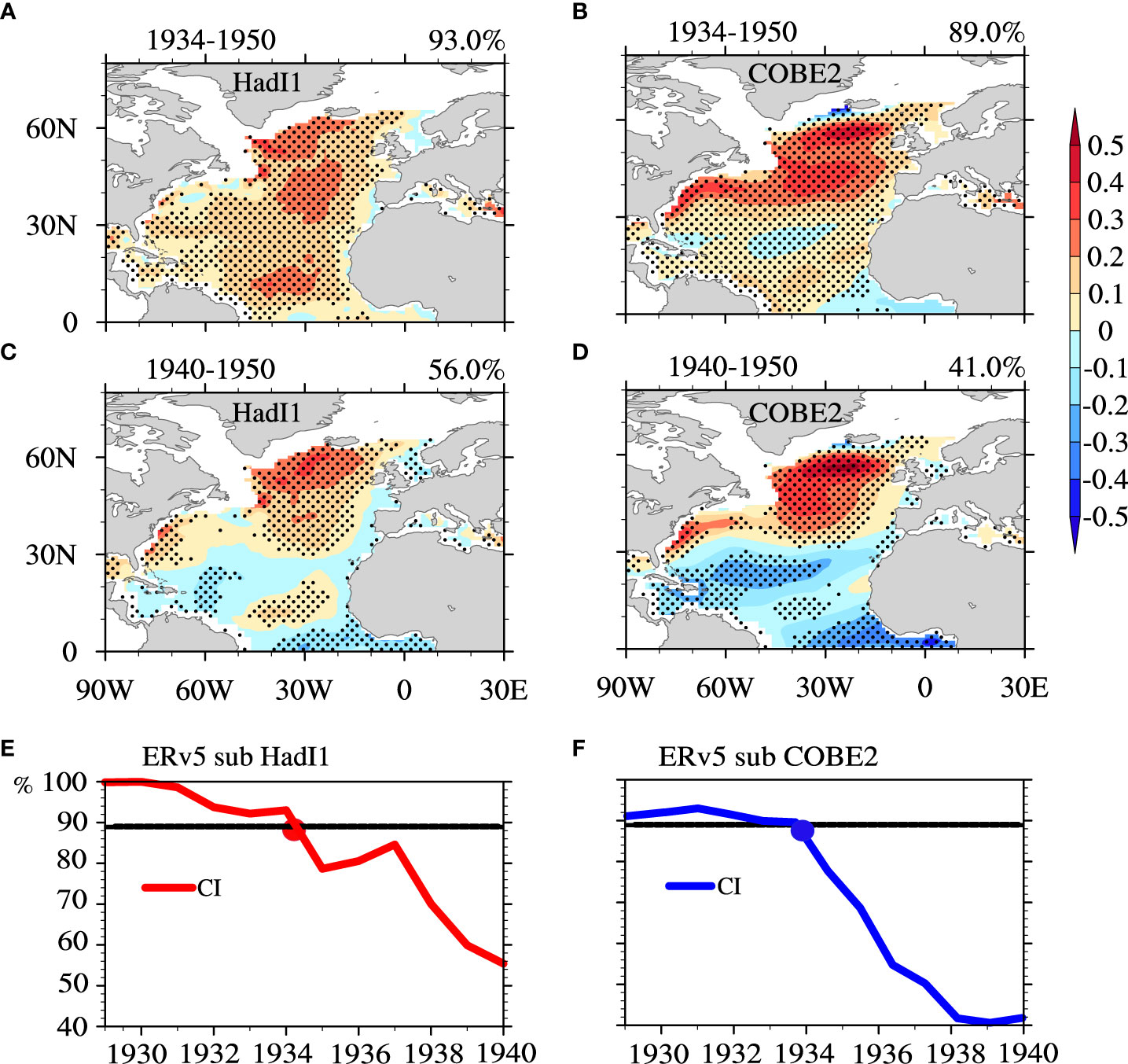
Figure 3 AMO patterns obtained from merged datasets based on LFCA. The merged datasets are obtained by replacing the SST data during 19xx–1950 in ERv5 with those in HadI1 (COBE2), where 19xx ranges from 1930 to 1940 in yearly increments and remains unchanged in other periods. (A, B) AMO patterns when 19xx is 1934 for HadI1 and COBE2, respectively. (C, D) As in (A, B), respectively, but when 19xx is 1940. (E, F) Change in the AMO CI as 19xx ranges from 1929 to 1940 when replacing HadI1 and COBE2, respectively. The x-axis denotes the period of replacement from 1929 to 1940. The dots in (E, F) are the positions where the CI value reaches the 89% level. Unit: °C.

The critical region generating the uncertainty in reproducing the coherent pattern of AMO

The period 1934–1950 includes the Second World War (1939–1945; hereafter referred to as WWII), during which the use of trade ships decreased sharply, resulting in a significant reduction in ship-based SST sampling. For example, all objectively analyzed SST datasets were based on version 3 of the International Comprehensive Ocean–Atmosphere Data Set or its earlier version (ICOADS, Freeman et al., 2017) before 1950, which mostly comprised ship-based observations. As shown in Figure 4A, these ship-based SST observations (data see DATA AND METHOD) were carried out along the trade routes between Europe and the Americas, with more than 20 SST samples per month along the busy routes, but only a few along the less busy routes before WWII. Then, the number of SST samples dramatically reduced during WWII (1940–1945), by over 50% in most regions (about 74% of the North Atlantic basin), and there was almost no SST sampling at all over the region of 0°–30°N and 0°–60°W (bounded by green lines in Figure 4B). Thereafter, the SST sampling size gradually recovered to, and even surpassed, the pre-WWII level (figure not shown), due to increased trade once again between Europe and the Americas. Therefore, we speculate that the more significant undersampling of SSTs during WWII has exerted a major influence on objectively analyzed SST datasets, and the methodologies used to derive these data have further transferred these influences into the AMO patterns and indices derived from the data.

FIGURE 4

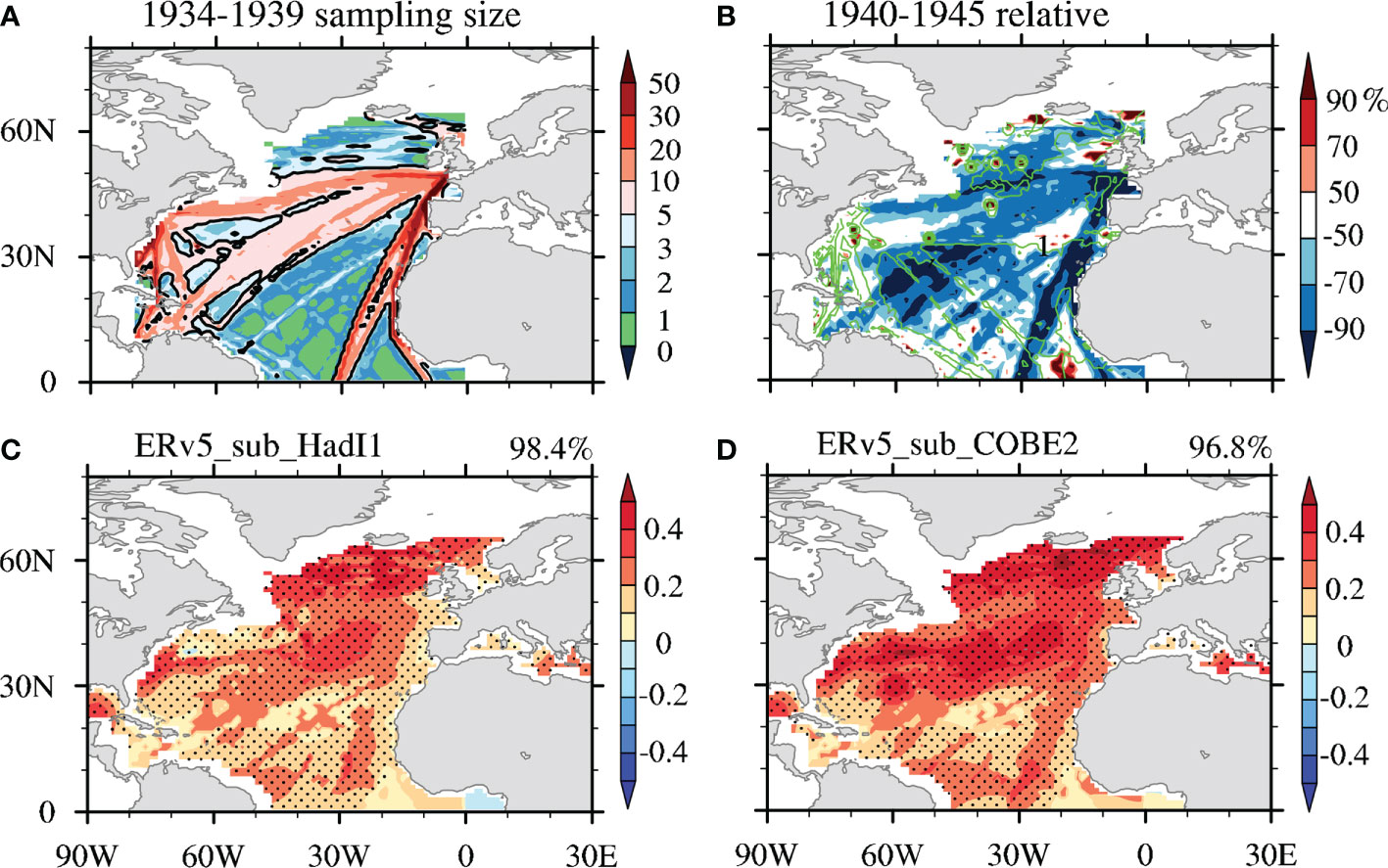
Figure 4 (A) The SST sampling size (unit:/month) during 1934–1939 and (B) the percentage change in the sampling size during 1940–1945 relative to that during 1934–1939. The green contour is the >1/month sampling size during 1940–1945. (C, D) The AMO patterns derived from merged SST data based on LFCA. The merged SST data are constructed by replacing ERv5 SST data with (C) HadI1 or (D) COBE2 SST data over the total region of sharply decreased sampling size [>50% in the colored region in (B)] during 1934–1950. The AMO CIs are shown in the top right. The unit for (C, D) is °C.

To further verify the effect of SSTs along the primary trade shipping routes on the resulting AMO pattern during WWII, we simply replace the ERv5 SSTs along these routes during 1934–1950 with those in the HadI1/COBE2 datasets, and then employ LFCA to extract the AMO. The resulting AMO spatial patterns are highly coherent, with CIs of 98.4%/96.8% after replacement with HadI1/COBE2 SSTs (Figures 4C, D). This confirms that the ERv5 SSTs along the primary trade shipping routes during 1934–1950 led to the incoherent AMO pattern (Figure 1A).

Impact of SST differences on the incoherent AMO pattern

To systematically examine the features of the SSTs along the primary shipping routes, we calculate the nonoverlapping piecewise area mean SST difference between ERv5 and HadI1 over the region where the sampling size decreased sharply (>50%) during 1940–1945 (Figure 4B), and the piecewise mean window is 6 years for the period 1922–1963, with a total of seven six-year intervals (Figure 5A). For the periods with plenty of SST samples (1922–1939 and 1946–1963), the area mean SST in ERv5 is systematically lower than that in HadI1 (Figure 5A). In contrast, for the period with a significantly reduced SST sampling size (1940–1945), the area mean SST in ERv5 is slightly higher than that in HadI1 (Figure 5A). These SST differences between ERv5 and HadI1 have also been found in previous studies (Kent et al., 2017; Kennedy et al., 2019; Chan and Huybers, 2021). In addition, the oscillation induced by these SST differences, as shown in Figure 5A during 1934–1950, may be artificial. Similar SST differences can also be found between ERv5 and COBE2 data for the same period (not shown). This suggests that the ERv5-based SSTs during the WWII period are biased toward being warmer than the SSTs in HadI1 and COBE2, and the resulting artificial SST oscillation may have contributed to the incoherent AMO spatial pattern, and the low coherence of the ERv5-based AMO index with the HadI1/COBE2-based AMO index.

FIGURE 5

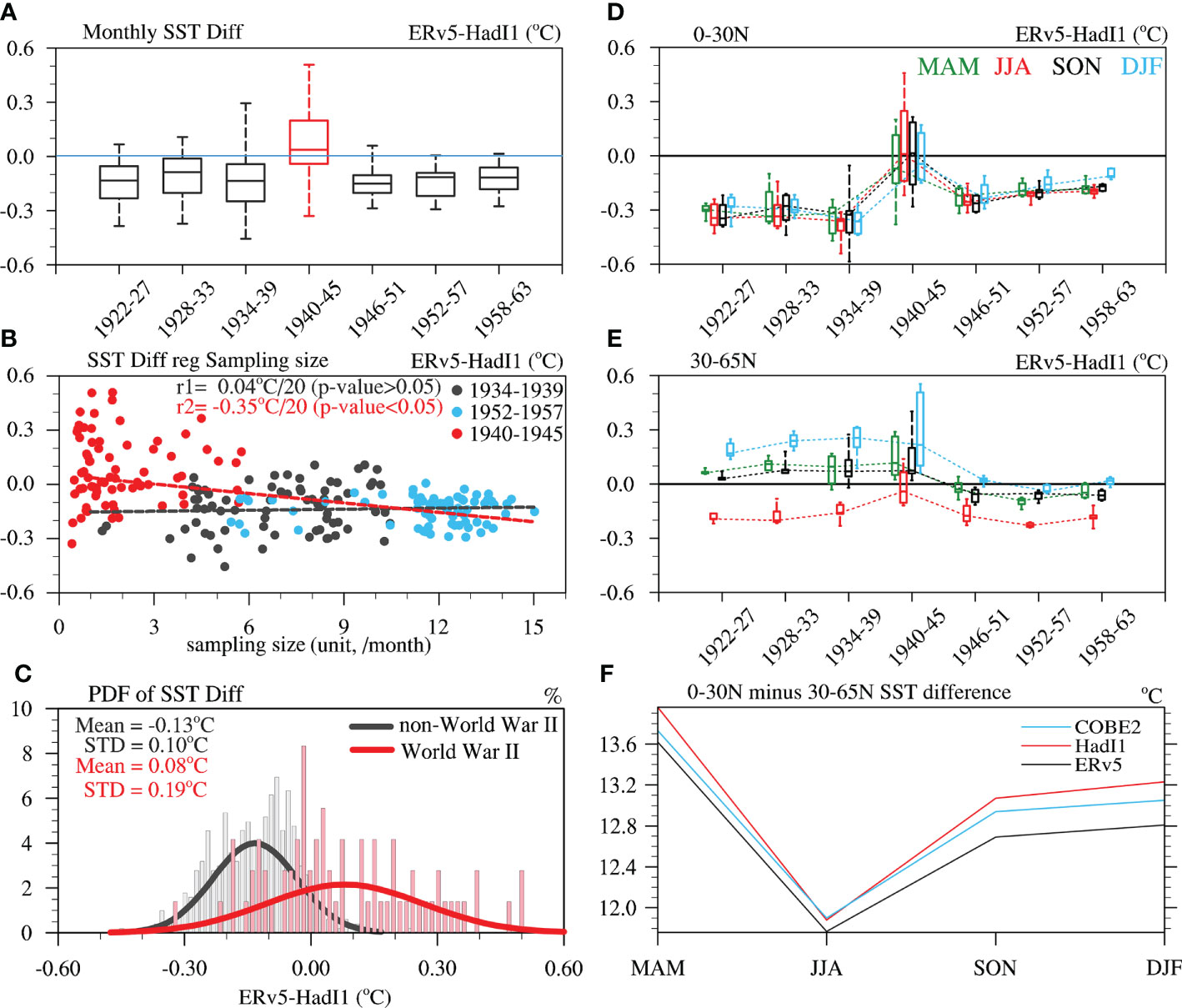
Figure 5 Relationship between SST differences (ERv5 minus HadI1) and the period of sampling size over the region of dark blue in Figure 4B during 1922–1963. (A) Box plot of monthly SST differences, in which the attributes in a box from top to bottom are the maximum, 75th percentiles, median, 25th percentiles, and minimum, respectively. (B) Sample size against averaged monthly SST differences over the same region as (A). Fitted values and p-values are also denoted in the figure. (C) probability density function (PDF) of randomly resampling the SST differences during the WWII period and non-WWII periods (i.e., pre- and post-war). The average and STD of the SST differences for different periods are given. (D, E) Boxplots of the SST difference (ERv5 minus HadI1) for four seasons over (D) 0°–30°N and (E) 30°–65°N. (F) Meridional SST difference between 0°–30°N and 30°–65°N for three SST datasets, measured by the averaged SST over 0°–30°N minus that over 30°–65°N for individual datasets.

To examine how the sampling sizes associated with bias-adjustment can affect the SST differences between ERv5 and HadI1, the monthly SST difference is regressed onto monthly sample sizes, and the probability density function is constructed based on the monthly SST differences between ERv5 and HadI1 in the periods during, before and after WWII (Figures 5B, C). In general, the mean SST differences have no obvious linear relationship with the sampling size before and after WWII (hereafter referred to as the dense sampling periods), such as regression coefficient is 0.04°C/20 sizes (p-value > 0.05) for 1934–1939 and 1952–1957. In contrast, the mean SST differences are negatively correlated with the sampling size for the period of analysis (Figures 5C), with a regression coefficient of −0.35°C/20 sampling sizes (p-value< 0.05). In fact, this negative correlation also appears in other periods including WWII (Table 2). These results imply that SST differences are strongly influenced by sampling size during the WWII. Meanwhile, the SST in ERv5 is colder than that in HadI1 by 0.13°C and with smaller spread [standard deviation (STD) = 0.10] during the dense sampling periods, but warmer by 0.08°C and with larger spread (STD = 0.19) during the WWII. Random resampling is used to test the significance of the differences between the means or STDs (Monte Carlo sampling test; see DATA AND METHOD), and the results show that the differences in SST mean values between the dense sampling periods (any 6 years within 1922–1939 and 1952–1963) and WWII (1940–1945) are statistically significant at the 95% level. Moreover, the differences between ERv5 and COBE2 are similar to those of HadI1 (not shown). Given the warming over the North Atlantic is weak during 1934-1960 (Figure 2D), it is suggested that North Atlantic SST anomaly on decadal time-scale mainly reflects AMO variability. Thus, the mean SST differences (ERv5 minus HadI1 or COBE2) between the dense sampling periods and WWII are significant, and capable of inducing a decadal oscillation that influence the AMO.

TABLE 2

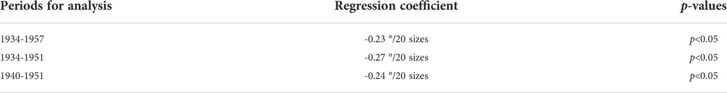
Table 2 The regression coefficient between the sample size and monthly SST difference (ERv5 minus HadI1) averaged over region where the sampling size decreased sharply (>50%) during 1940–1945 for different periods.

As ERv5, although HadI1 and COBE2 also share the same raw observational data source in ICOADS, the different bias adjustment schemes applied in these datasets may affect the resulting SST and its variability. The HadI1/COBE2 datasets adopt a simplified physical model of buckets (Rayner et al., 2003; Hirahara et al., 2014) based on the scheme of FP95 (Folland and Parker, 1995) to correct the systematic cooling due to wind and solar insolation at the sea surface (Folland et al., 1984; Folland and Parker, 1995). In ERv5, meanwhile, the bias adjustment is the approach of SR02 (Smith and Reynolds, 2002), which is based on the statistical relationships between nighttime marine air temperature and SST (Huang et al., 2017). The SR02 bias adjustment has more obvious seasonal differences than that of FP95 (Smith and Reynolds, 2002). In the following, by applying LFCA to the seasonal mean ERv5 SST over the entire North Atlantic, we examine whether this SR02-related seasonal difference affects the AMO pattern. As shown in Figure 6, the AMO pattern derived in June–July–August (JJA) is highly spatially coherent, with a CI of 99% (Figure 6A), while the AMO pattern derived in September–October–November (SON) season is not coherent over the entire North Atlantic, with a low CI value (51%; Figure 6B). Although the CIs are higher for the AMO patterns derived in March–April–May (MAM) and December–January–February (DJF) than SON, they are still lower than the 89% threshold (Figure S2). However, the AMO patterns extracted from the seasonal mean HadI1/COBE2-based SST are coherent over the entire North Atlantic, with CIs higher than 89% (not shown). This indicates that the seasonal SST differences used in ERv5 do contribute to the incoherent AMO patterns, except in JJA.

FIGURE 6

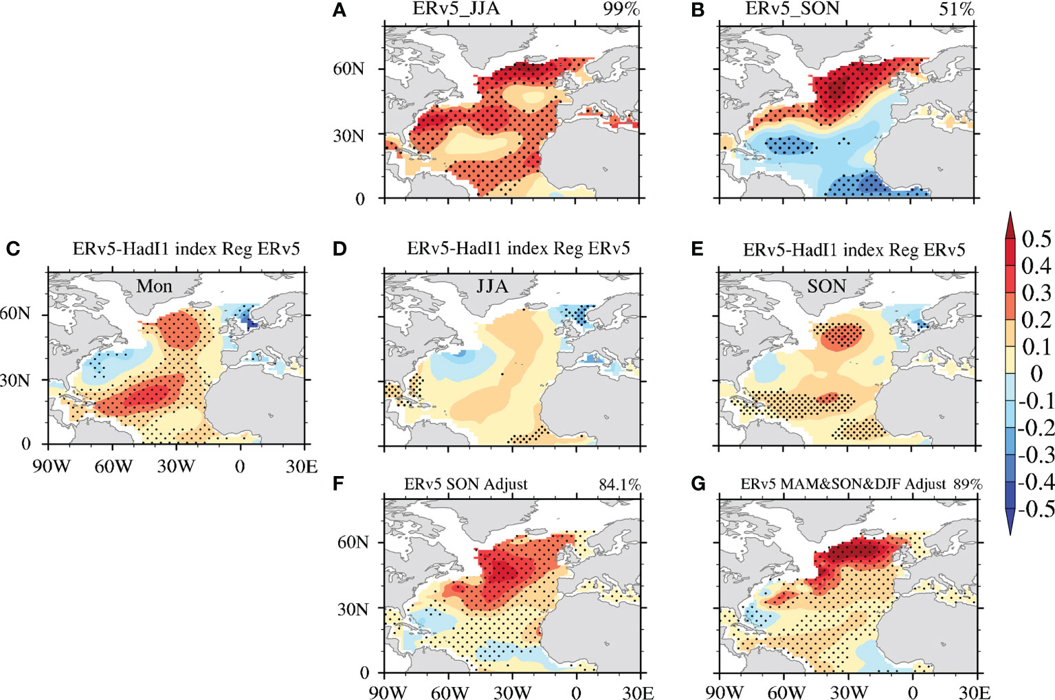
Figure 6 The AMO pattern extracted from the seasonal mean ERv5 SST in (A) JJA and (B) SON during 1900–2019 by LFCA. (C–E) Regression patterns of the ERv5 SSTA onto the difference (ERv5 minus HadI1) in the AMO index (defined by the averaged SSTA in the North Atlantic) with a 6-year running mean for the (C) monthly, (D) JJA, and (E) SON data during 1934–1950. (F, G) The AMO pattern extracted from the adjusted (F) SON and (G) monthly ERv5 data during 1900–2019 by LFCA. The adjusted SON ERv5 data in (F) are obtained by first removing the SON seasonal SST difference (ERv5 minus HadI1) from the monthly ERv5 data during 1934–1950, and then computing the SON seasonal mean SST during 1900–2019. The adjusted monthly ERv5 data in (G) are obtained by removing the MAM, SON and DJF seasonal SST differences from the monthly ERv5 data during 1934–1950. The AMO CI value is given in the top right. The dots indicate statistical significance at the 95% confidence level.

To investigate why seasonal SST differences contribute to the incoherent AMO pattern in ERv5, we calculate the seasonal mean SST difference (ERv5 minus HadI1) over the extratropical North Atlantic (30°–65°N), tropical North Atlantic (0°–30°N), and the seasonal mean meridional SST contrast for different datasets (Figure 5). In general, the seasonal mean SST differences between ERv5 and HadI1 present low–high–low oscillations over the entire North Atlantic (0°–65°N) during 1934–1951 (not shown). These oscillations become more obvious in the tropical North Atlantic, but less so in the extratropical North Atlantic. Before 1940, the median SSTs in ERv5 are about 0.3°C colder than those in HadI1 in all seasons in the tropical North Atlantic, but 0.05°C–0.3°C warmer in the extratropical North Atlantic, except in JJA. Thus, this warmer SST in the extratropics and colder one in the tropics in ERv5 relative to HadI1 lead to large meridional SST differences in all seasons except JJA before 1940. These meridional SST differences also exist after 1945, but are smaller due to the smaller cooling difference in the tropics and slightly larger cooling difference in the extra-tropics (Figures 5D, E). In contrast, in JJA, these meridional SST differences are very small because of similar behavior between the tropical and extratropical North Atlantic (Figures 5D, E). This leads to the smallest meridional SST contrast existing in JJA during 1934–1950 in ERv5 (Figure 5F). This corresponds to the smaller correction in boreal summer than other seasons in the bias adjustment of SR02 (see Figures 6, 7 in Smith and Reynolds, 2002). Therefore, although the low–high–low oscillation of the SST difference between ERv5 and HadI1 is artificial, the enlargement of the meridional SST contrast between the tropical and extratropical North Atlantic is the possible cause of the incoherent AMO pattern in MAM, SON and DJF, and the monthly mean.

FIGURE 7

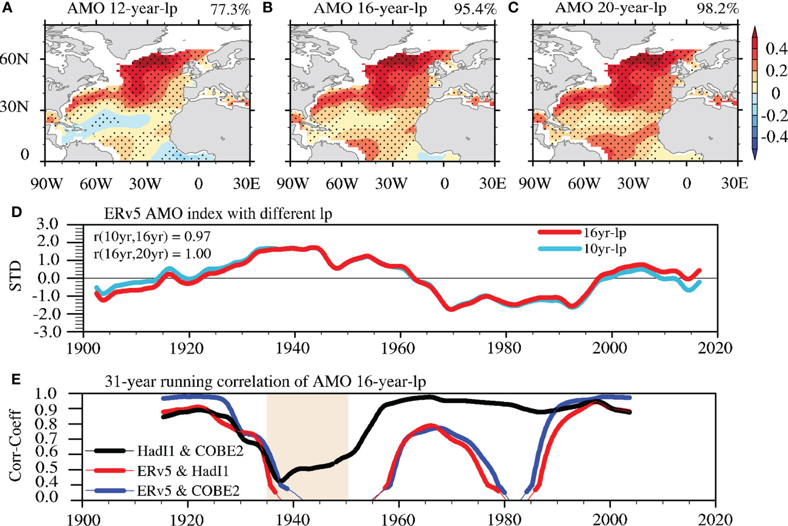
Figure 7 The AMO pattern extracted by LFCA from ERv5 with three low-pass filter frequencies: (A) 12 years, (B) 16 years, and (C) 20 years in LFCA (40 EOFs are also applied). Dots indicate where values pass the 95% significance level, and the AMO CI is denoted in the top right. (D) AMO indices with different low-pass filter frequencies, and their TCCs are given. (E) Similar to Figure 2C but the AMO is extracted using a 16-year low-pass filter. The unit in (A–C) is °C.

To examine whether spatial differences in the seasonal ERv5 SST affect the resulting AMO patterns, we regress the monthly or seasonal mean ERv5 SST onto the difference between the ERv5-based and HadI1-based AMO indices (defined by the area-weighted averaged SST over the North Atlantic) with a six-year running mean during 1934–1950 (Figures 6C–E). For the monthly regression, the monthly SSTs are significantly related to the differences in the AMO indices in most parts of the North Atlantic (Figure 6C; stippling indicates a regression significant at the 95% level). For SON, although the regions with significant regression become smaller, the overall regression pattern is similar to that for the monthly SST (Figure 6F). On the other hand, the regions with statistically significant regression are negligible in JJA (Figure 6D). This indicates that the ERv5 SST in JJA (SON) is not related (related) significantly with the difference in the AMO. By removing the spatial effect of the SST difference (ERv5 minus HadI1) in SON from the monthly ERv5 data during 1934–1950, the extracted AMO pattern in the seasonal SON mean is almost coherent, and the CI increases from 51% (Figure 6B) to 84.1% (Figure 6F). Furthermore, the extracted monthly AMO pattern is also coherent after removing the spatial SST effects (ERv5 minus HadI1) in MAM, SON and DJF from the monthly ERv5 data (Figure 6G). Thus, the spatial distribution of the seasonal mean SST affects the AMO pattern greatly, with a coherent (incoherent) AMO pattern in JJA (SON).

Impact of low-pass filtering on the incoherent AMO pattern

The other difference in the bias-adjustment process is the employment of a Lowess filter (Cleveland, 1981) to maintain the signal continuity around the 1940s in ERv5, and this filter is equivalent to a 16-year low-pass filter (Huang et al., 2015). As described in previous studies (Wills et al., 2018; Wills et al., 2019), LFCA uses a 10-year Lanczos low-pass filter to extract the SST variability on decadal timescales, and the mismatch between this and the Lowess filter can lead to spurious signals. Frankignoul et al. (2017) also indicated this smoothing in bias adjustment can influence the resulting AMO pattern. To examine this mismatch, the AMO pattern and index are extracted using LFCA by applying low-pass filters with windows of 12, 16 and 20 years. As shown in Figures 7A–C, the coherence of the AMO spatial pattern is progressively better as the low-pass filter window increases, e.g., with a CI of 77.3% for a 12-year low-pass filter, and 95.4%/98.2% for a 16/20-year low-pass filter, over the North Atlantic (Figures 7A–C). Besides, the original low–high–low oscillation between ERv5 and the other SST datasets (Figure 5A) disappears once 16-year low-pass filter is applied (not shown). Further analysis indicates that by using a fixed number (35) of empirical orthogonal functions (EOFs) in LFCA, the CIs of the AMO pattern in ERv5 increase gradually as the low-pass filter window lengthens from 10 to 25 years, from a CI below 70% to over 90% (Figure S3). The sensitivity of the resulting AMO pattern to the different filter window lengths is significantly less for the HadI1 and COBE2 SSTs, since the CIs are always higher than 90% when using the same number of EOFs as for the ERv5 SSTs. Therefore, we conclude that to obtain a spatially coherent AMO pattern from ERv5 data, a low-pass filter window equal to or longer than 16 years is needed, but this requirement is not needed for HadI1 and COBE2 data.

With this improved AMO pattern by applying a low-pass filter of 16 years or longer to ERv5 data, the question naturally arises as to whether this might lead to variation in the AMO index derived from ERv5 that is more coherent with those derived from HadI1 and COBE2 data. As shown in Figure 7D, the resulting AMO indices with a 10- or 16-year low-pass filter are nearly identical, with a correlation coefficient of 0.97. The same is true for the AMO indices derived from HadI1/COBE2 (not shown). As expected, when the 31-year running TCC is calculated between the AMO indices derived from ERv5 and those from HadI1/COBE2 by using a 16-year low-pass filter, these indices are still uncorrelated during 1940–1950 (Figure 7E). This indicates that, although different filters can significantly improve the spatial coherence of the resulting AMO patterns from ERv5, their influence on the temporal evolution of the AMO index is negligible.

Warming trend over the North Atlantic and the AMO

To properly obtain the AMO, the response of the SST to external forcing (e.g., greenhouse gases) needs to be removed. For LFCA, the assumption is that this SST response is heterogeneous spatially. The more traditional approaches, however, such as that of Trenberth and Shea (Trenberth and Shea, 2006; TS2006 hereafter), assume a globally uniform response, and the externally forced trend is represented by the global mean SST. To test whether these different assumptions affect the resulting AMO patterns derived from ERv5 data, we first remove the global mean SST at each grid point (i.e., detrended SST), and then define the AMO index as the area-weighted North Atlantic SST based on the detrended SST (the same as with TS2006), and the AMO pattern as the regression of this AMO index onto the detrended SST, or by applying LFCA to the detrended SST (hereafter, GM_LFCA). Both approaches result in a much improved spatial coherence of the AMO pattern, with a CI of 99.9% when the AMO index is defined as the area-weighted detrended SST (Figure 8A vs. Figure 1A) and a CI of 91.0% when the AMO pattern is derived from detrended SST using LFCA (Figure 8B vs. Figure 1A). This indicates that different assumptions regarding the SST’s response to changes in external forcing can also affect the resulting AMO patterns derived from ERv5 and, to a lesser degree, this may also be true for the other two datasets. On the other hand, the second LFCA mode derived from the detrended SST shows a pattern similar to the regional SST response to the external forcing (Figure 8C), and the subpolar North Atlantic warming hole is possibly associated with the AMOC slowdown (Caesar et al., 2018). The trend of this second LFCA mode (1.31 STD/100 years) is statistically significant according to the Mann–Kendall (MK) trend test (see DATA AND METHOD), and thus this second mode represents the residual of the warming trend in the North Atlantic. However, the AMOs derived from the other two SST datasets (HadI1/COBE2) are not sensitive to whether or not the globally uniform forced trend is removed before the application of LFCA (figure not shown). Thus, only the AMO pattern derived from ERv5 is sensitive to how the externally forced SST trend is represented, i.e., spatially uniform or heterogeneous.

FIGURE 8

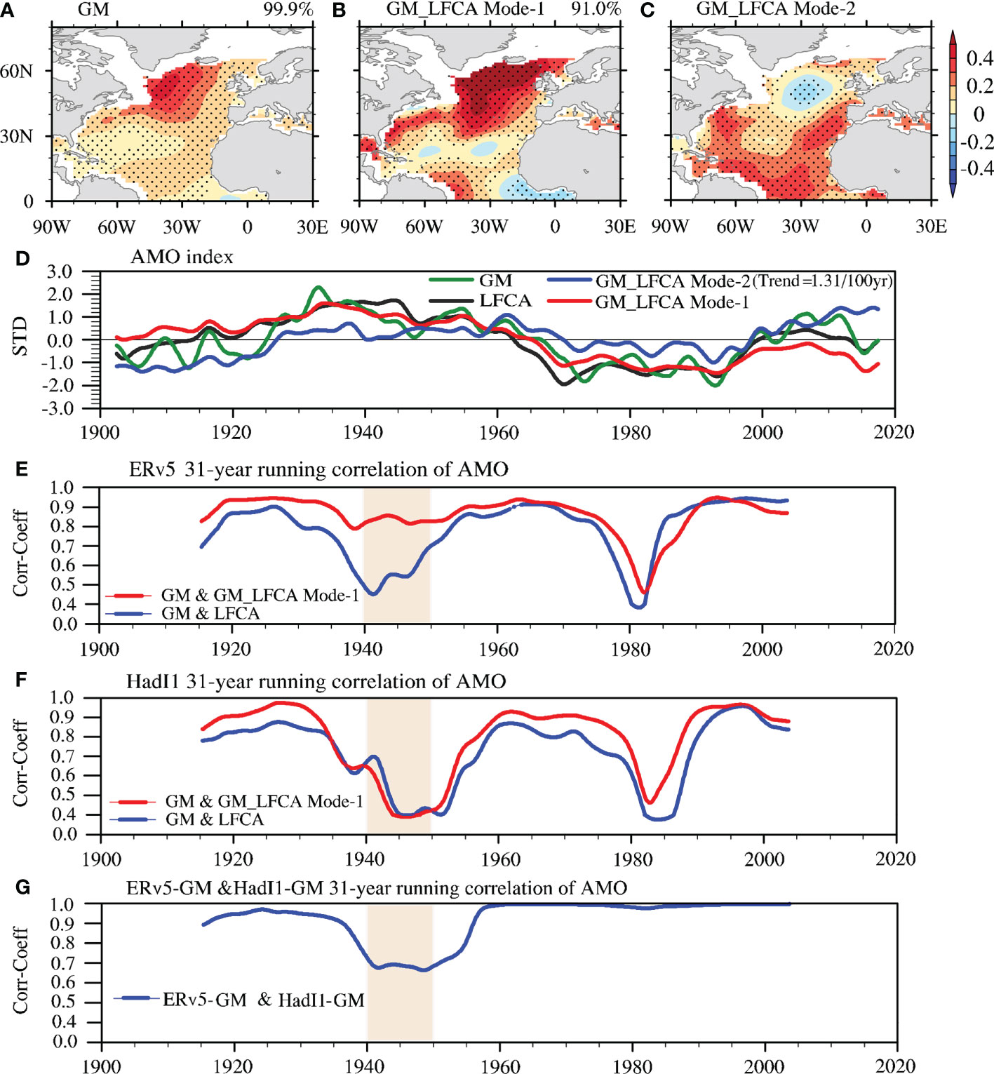
Figure 8 The AMO patterns (A) using the definition of subtracting the global mean SST (GM) based on TS2006 and (B) extracted by LFCA before removing the global mean SST (GM_LFCA Mode-1). Dots indicate where values pass the 95% significance level, and the AMO CI is given in the top right of the figure. (C) Second leading GM_LFCA Mode (GM_LFCA Mode-2). (D) AMO indices derived from LFCA, GM, GM_LFCA Mode-1 and GM_LFCA Mode-2 based on ERv5 SST data. (E) Similar to Figure 2C but for different approaches based on ERv5. (F) Similar to (E) but based on HadI1. (G) Similar to (E) but using the TS2006 approach based on ERv5 and HadI1.

Comparison among the spatial patterns and time series of the first leading LFCA modes (i.e., North Atlantic warming) in these three datasets shows high spatial and temporal consistency, with PCCs ≥ 0.97 and TCCs ≥ 0.9. Therefore, this warming trend is not likely the cause of the low coherence in the AMO pattern derived from ERv5. However, when the first leading EOF mode (long-term heterogeneous warming pattern) is removed from the SST by linear regression and LFCA is applied to the residual SST, the spatial coherence of the resulting AMO pattern becomes even lower for ERv5 (41.6% in Figure 1F vs. 69.2% in Figure 1A). Similar results are also found for the other two datasets (Figure S4). This suggests that the heterogeneous North Atlantic warming pattern can contribute positively to the AMO spatial coherence for all datasets.

Next, we look at the effects of these different detrending methods on the resulting AMO indices. As shown in Figures 8E, F (blue lines), the AMO indices obtained from LFCA differ significantly from those obtained from the TS2006 method around 1940 and 1980 for both the ERv5 and HadI1 datasets, suggesting that different assumptions in the North Atlantic SST response to global warming can result in different temporal evolutions in the AMO index around 1940 and 1980. As the spatially uniform warming is removed, the GM_LFCA Mode-1 indices still differ from those based on TS2006 (red lines in Figures 8E, F) around 1940 and 1980, especially in HadI1. This indicates that, with the removal of the same spatially uniform warming trend, spatially uneven warming trends are left (Figures 8C, D), which may explain the differences among the AMO indices obtained from the TS2006 and GM_LFCA methods (Figures 8D, E). Even if the TS2006 method is applied to both ERv5 and HadI1, the resulting AMO indices are different around 1940 (Figure 8G). This implies that a fundamental difference exists around 1940 between ERv5 and HadI1. Potentially, there might be other reasons behind the inconsistencies in the AMO indices between ERv5 and the other two datasets around 1940 and 1980, but we leave these to be investigated in a future study.

Influence of ocean and atmosphere in shaping the coherent pattern of AMO

Here we have used the piControl experiment of CESM2 and its constructed ensemble (see DATA AND METHOD) to investigate the possible role of ocean and atmosphere in shaping the coherent pattern of AMO. The LFCA is applied to the constructed ensemble member from the piControl run to compute AMO. Figure S6A shows the correlation coefficient between AMO in the ensemble member and AMO from each of three SST datasets (ERv5, HadI1, and COBE2). By considering correlation coefficient of AMO index and CI of AMO pattern, we selected the member that resembled the one in three observed SST datasets most. The correlation coefficient is 0.71 (0.57/0.64, p-value<0.05) between AMO index in the ensemble member and AMO index in ERv5 (COBE2/HadI1), and related AMO patterns are shown in Figure S6. The ERv5-like member shows an incoherent AMO pattern (CI=71%), while both COBE2-like and Had1-like members show a coherent AMO pattern (CI=88% and 91%, respectively), indicating that these three members are good representation of the observational AMO pattern/index derived from the three datasets.

Based on SST tendency equation (see DATA AND METHOD) proposed by Zhang et al. (2016), we diagnosed the relative contribution of net surface heat flux Q'_net and oceanic heat transport convergence OHTC' n shaping the tendency of decadal variability of SST. The SST tendency, Q'_net and OHTC' (OHTC^′ $\approx {\rho }_0{C}_{p}h\frac{dSST\prime }{dt}-Q{\prime }_{net}$) regressed on the AMO index at a 2-year leading time (the maximal correlation between the tendency of AMO index and AMO index, Figure S7), respectively (Figure 9). The atmosphere seems to drive the variation of SST tendency in the ERv5-like member as the OHTC is almost in balance with Q'_net and SST tendency is weak over the North Atlantic prior to the maximal positive phase of AMO. In contrast, in the COBE2-like or Had1-like members, the OHTC contributes to the warming SST tendency over the subpolar North Atlantic, where the upward Q'_net can directly balance SST, indicating that the atmosphere is passively responded to SST warming. Previous study of observational surface heat flux also supports the ocean active role in AMO (Gulev et al., 2013).

FIGURE 9

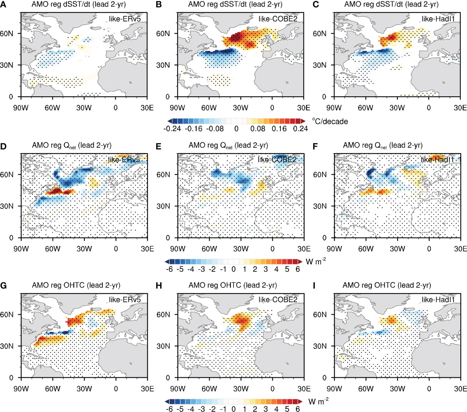
Figure 9 The (A, D, G) SST tendency, (B, E, H) net surface heat flux Q'_net, and (C, F, I) oceanic heat transport convergence OHTC', regressed on the AMO index in selected members of CESM2 piControl with a 2-year lead time, respectively. The downward direction is positive for Q'_net.

Above analysis indicates that the SST anomaly can serve as a perturbation to the interaction within ocean and atmosphere, and thus can influence which of ocean and atmosphere in dominating the AMO tendency, and finally the AMO.

Conclusion and discussion

In this study, we investigate the uncertainty in the resulting AMO indices and spatial patterns arising from the differences in reconstructed SST observations (ERv5, COBE2, and HadI1) over the North Atlantic from 1900 to 2019 by applying the same methodology—namely, the LFCA method. Three indices (CI, PCC and TCC) are used to quantify the consistency among the AMO patterns and indices derived from the different datasets. Instead of the commonly accepted basin-wide spatially coherent pattern over the North Atlantic (Zhang et al., 2019), the extracted AMO pattern from the ERv5 dataset is not spatially coherent, with a negative anomaly over the subtropical North Atlantic in the AMO’s positive phase. The ERv5 AMO index is decorrelated with the HadI1/COBE2 AMO indices during 1934–1950 owing to its preceding 10–15 years. Thus, we conclude that the AMO properties in ERv5 differ significantly from those in the other two datasets.

Further analysis reveals that the sensitive region and period of the ERv5 SST data for the AMO pattern are the shipping routes in the North Atlantic during 1940–1945 (WWII), in association with sharply decreased sample sizes. These SST differences introduce a spurious artificial interdecadal oscillation during 1934–1950.

This artificial oscillation is firstly related to the seasonal SST differences stemming from the different bias-adjustment schemes employed in ERv5 and HadI1/COBE2. The bias-adjustment scheme used in ERv5 leads to higher corrected SSTs in the extratropics in MAM, SON and DJF than in JJA before the 1950s. This results in increased meridional SST gradients between the extratropics and tropics (warming SSTAs in the extratropics and cooling ones in the tropics) in MAM, SON and DJF. These are likely to serve as initial perturbations in the air-sea interaction by firstly influencing the wind or heat/water fluxes over the North Atlantic, and then wind can affect the change of SST by oceanic general circulation or affect SST directly. Given that ocean deep convection (denoted deep mixed layer) frequently appearing in cold seasons (such as SON, DJF or MAM) over the North Atlantic (e.g., Alexander and Deser, 1995), SST anomalies can have potentially footprinted on ocean deep convection by wind or heat/water flux, and further joined in the deep ocean circulation process, which contribute to the decadal SST variability over the North Atlantic. So, this bias-adjustment can stimulate the enhanced artificial oscillation and resulting incoherent AMO pattern based on the seasonal mean SSTs in MAM, SON and DJF but not in JJA. Such differences further cause the incoherent AMO pattern extracted by LFCA based on the monthly ERv5 SST. By contrast, the bias adjustment is almost the same between HadI1 and COBE2 in the early periods, which leads to the consistent SST variations (Huang et al., 2015).

This artificial oscillation may also be related to the 16-year low-pass filter employed in the bias-adjustment process used in ERv5. This low-pass filter is mismatched with the 10-year low-pass filter used in LFCA and the traditional definition. Thus, the AMO pattern derived from the ERv5 dataset is affected by the low-pass filter in the bias adjustment.

The assumed pattern of North Atlantic warming in response to changes in external forcing can influence the resulting AMO patterns, especially for the ERv5 dataset. The coherence of the AMO patterns is low (high) when the warming pattern is assumed to be uneven (even). The resulting AMO indices derived from different methods (TS2006, LFCA, TS2006_LFCA) show significant differences during 1940–1950 for the same dataset (e.g., ERv5 or HadI1); and for the same methods (LFCA or TS2006), the AMO index from ERv5 is significantly different from that derived from HadI1 or COBE2. It is worth noting that we can improve the coherence of the AMO pattern in ERv5 by using a low-pass filter frequency that is consistent with that used to construct the ERv5 SST dataset, but not the AMO index during 1940–1950.

The SST datasets used in previous analyses have employed different versions of ICOADS. For example, COBE2 and its earlier version, COBE-SST (Ishii et al., 2005), used ICOADS 2.5 and ICOADS 2.0 (Woodruff et al., 2011), respectively, and ERSST employed ICOADS 3.0 for v5 (Huang et al., 2017), 2.5 for v4 (Huang et al., 2015), and 2.1 for v3 (Smith and Reynolds, 2003). The AMO patterns extracted from COBE-SST and COBE2 are coherent over the North Atlantic, with high CIs (>89%). On the other hand, the AMO patterns extracted from ERSST.v3 and ERSST.v4 using LFCA are also unable to show a coherent warming in the North Atlantic, with low CIs—the same as that from ERv5 (Figure S5). This indicates that different versions of the ICOADS data is not the source of different coherence in the AMO patterns between ERv5 and HadI1/COBE2. The corrected ICOADS from Chan and Huybers (2021) is employed to obtain the AMO pattern, as the coherent (incoherent) AMO pattern is derived from HadI1 (ERv5) merged with the corrected ICOADS (not shown), which indicates the corrected sources do not significantly influence the AMO pattern, but the bias adjustment in ERv5 does play a crucial role.

Uncovering the role of observational SST uncertainty that was resulted from mid-20th century bias adjustment in the observed AMO will help to understand the influence of ocean/atmosphere in shaping the AMO. It is shown that the ocean heat transport convergence seems to drive the tendency of AMO in a coherent AMO pattern (like COBESST2 or HadISST1). In contrast, in the incoherent AMO pattern, the atmosphere may become the driver of the AMO tendency.

Finally, two suggestions for how to obtain a more coherent AMO pattern from ERv5 data are noted, as follows. First, to obtain the coherent warming AMO pattern using LFCA over the North Atlantic, it is necessary to preprocess the monthly SST to an annual SST to cancel out the seasonal difference due to the bias correction. And second, if monthly SST data are employed, a 16-year low-pass filter is recommended in LFCA.

Data and method

Datasets

Four different monthly reconstructed SST datasets are employed, including ERv5 (Huang et al., 2017), COBE2 (Hirahara et al., 2014), HadI1 (Rayner et al., 2003) and COBE-SST (Ishii et al., 2005). The resolutions of these SST products are all 1° × 1°, except ERv5 (2° × 2°), the data of which are bilinearly interpolated into a resolution of 1° × 1° to keep the same resolution as the other datasets. This interpolation does not influence our results. The monthly SST climatology for 1971–2000 is removed to obtain the SSTA. The SSTA is employed in LFCA or a substitutive process in the figures, except in Figure 5 (using SST) in the main text. Version 3.0 of ICOADS (Freeman et al., 2017) with quality-control (Chan et al., 2019) is used to compute the sampling sizes of the observational SST. OISSTv2 (Reynolds et al., 2007) is used to prove that the post-1980s SST data do not reduce the CI of the AMO in Figure 1.

Because of the large uncertainty before 1900 (Folland et al., 2001), the SST data before this point are excluded from this study of the AMO. HadI1 sea-ice concentration data (Rayner et al., 2003) are also used for masking where the sea-ice’s concentration is positive, as recommended in Drews and Greatbatch (Drews and Greatbatch, 2016), to exclude the influence of sea ice in our results.

The piControl experiment with external forcing fixed at 1850 level of CESM2 (Danabasoglu et al., 2020) for 200-1200 year is used. The horizontal resolution of atmosphere component is 1.25° ×0.9˚, and that of ocean component is about 1.125° × 0.44°. Previous studies show that CESM2 well reproduce some characteristics of observed AMO (Deser and Phillips, 2021). The model data anomaly is obtained by subtract the climatology of the whole time period, and data is also linearly detrended to remove the climate drift. To compare with the observation (whose length of data record is about 120 years), we created surrogate ensembles from the piControl. The 89 ensemble members with the length of 120 years are created by selecting 200-319, 210-329, 220-339, ... , 1080-1199 year from the piControl run, respectively. As the external forcing is a constant, the first leading low-frequency mode was extracted from SST anomaly over the North Atlantic (0-65 ˚N) based on LFCA (Low Frequency Component Analysis, introduced in the next) method for each member. The first leading LFCA mode is AMO.

Low frequency component analysis

LFCA (Wills et al., 2019) aims to find low-frequency variability by solving linear combinations of several leading EOFs that maximize the ratio of low-frequency to total variance. Here, the low-frequency variance represents a “signal” that exists within the internal variability or between realizations. Thus, LFCA is similar to maximizing EOF analysis using the signal-to-noise ratio (Schneider and Held, 2001). On a longer timescale, the SST response to external forcing can be distinguished from internal variability based on maximizing the ratio of low-frequency to total variance. For instance, the AMO (or the Pacific Decadal Oscillation) have been isolated from global warming based on SST in LFCA (Wills et al., 2018; Wills et al., 2019). Compared with other methods, the advantage of LFCA is that it can extract low-frequency signals, such as the AMO, without the need to assume the spatiotemporal structure of global warming in advance. A short introduction to the algorithm is provided as follows:

LFCA is dependent on (1) the number of EOFs, (2) the temporal length of the low-pass filter, and (3) the input data matrix that has temporal and spatial dimensions (e.g., SST). Here, we use Lanczos filtering with a 10-year low-pass filter to extract the signal on decadal timescales (i.e., the AMO). The number of EOFs is set to capture at least 85% of the total North Atlantic SST variance, as done in Wills et al. (2019). Here, we use 35 EOFs to obtain the AMO. The influence of the number of EOFs on the extracted AMO CI is tested (Figure S1), and it is shown that the average CI value for the AMO in COBE2 or HadI1 is 89%, which is set as a threshold for judging a coherent AMO pattern in this study. More details of this method can be found in Wills et al. (2019).

In this study, LFCA is applied to the monthly SST in the North Atlantic between 0° and 65°N, which is consistent with the traditional definition (Zhang et al., 2019). Unless otherwise mentioned, the Atlantic domain between 0° and 65°N is used throughout the study. The domain is different from that employed in Wills et al. (2019). Many factors can influence the definition of the AMO pattern/index, such as the detrending method (Ting et al., 2009; Frankignoul et al., 2017; Yan et al., 2019; Deser and Phillips, 2021) or the region used for the definition, as no single physical mechanism explains the regional definition of the AMO (Wills et al., 2019). Our study aims to clarify the influence of historical SST uncertainty in the North Atlantic on the extracted AMO, which has typically been ignored in previous studies. Thus, we use the traditional domain (0°–65°N) to exclude the possible influence of the domain definition.

AMO index based on TS2006

Following a traditional method (Trenberth and Shea, 2006, TS2006 herafter), we define the AMO index as the low-frequency component of the difference between the area-weighted mean SSTs in the North Atlantic (0°–65°N, 0°–80°W; NASSTA) and the global domain (60°S–60°N). Then, a low-pass filter with a window of 10 years is applied to obtain the low-frequency component (i.e., the AMO). This AMO index is compared with the AMO index derived from LFCA in Figure 8.

Coherence index, pattern and temporal correlation coefficient

Here, we define a CI as the ratio of the area where the SSTA is greater than zero in the North Atlantic to the total area in the North Atlantic during the AMO’s positive phase. Thus, the CI denotes the areal extent of coherent warming in the North Atlantic related to the AMO:

$\begin{array}{ll}CI=\frac{{\sum }_{NA}Are{a}_{i,j}(AMO>0,SSTA>0)}{{\sum }_{NA}Are{a}_i{,}_j}\times 100\%& (1)\end{array}$

The numerator in the above formula is the area with positive SSTAs in the North Atlantic during the AMO’s positive phase, and the denominator is the total area of the North Atlantic. NA denotes the North Atlantic, and Area_i,_j is the area of a grid cell.

The warming pattern for the AMO has a spatial gradient, such as the stronger signal over the subpolar North Atlantic and the weaker signal over the low latitudes in observations (Zhang et al., 2019). Here, we compare the PCC of the AMO in different datasets to quantify the similarity of the spatial gradient in the AMO:

$\begin{array}{ll}PC{C}_{NA}=\frac{Co{v}_{NA}(AM{O}_{X}AM{O}_Y)}{\sqrt{Va{r}_{NA}(AM{O}_X})\sqrt{Va{r}_{NA}(AM{O}_Y})}& (2)\end{array}$

where AMO_X and AMO_Y are the spatial values of the AMO patterns in its positive phase from two different datasets; Cov_NA denotes the covariance; and Var_NA(AMO_X) and Var_NA(AMO_Y) are the corresponding variances.

The TCCs between the AMO indices from different datasets are calculated in a similar way to the above PCC formula, where AMO_X and AMO_Y are the AMO indices from two different datasets, respectively.

Mann–kendall trend test

To investigate the statistical significance of the linear warming trend, we apply the rank-based non-parametric MK test (Mann, 1945). The MK test is mathematically defined as

$\begin{array}{ll}S={\sum }_{i=1}^{n-1}{\sum }_{j=i+1}^{n}sgn(X_j-X_i)& (3)\end{array}$

where n is the size of the time-series data, and X_i and X_j are data in the ith and jth times series, respectively (i< j). sgn(X_j − X_i) can be three different values: −1 if X_j − X_i < 0; 0 if X_j − X_i= 0; and +1 if X_j − X_i > 0. For large datasets (here, n = 1440), the S statistic is normally distributed with zero mean. If E(S) is the mean and V(S) is the variance of S, a standard normal test statistic is defined as (Bisht et al., 2018)

$\begin{array}{ll}Z=\{\begin{array}{l}\frac{S+1}{\sqrt{V(S)}},ifS<0\\ 0,ifS=0\\ \frac{S-1}{\sqrt{V(S)}},ifS>0\end{array}& (4)\end{array}$

As the Z computed for time-series of GM_LFCA Mode-2 (Figure 7D) is 16.8, which is much larger than the a = 0.05 significance level ( Z_a = 1.96), suggesting a significant warming trend of GM_LFCA Mode-2.

Sen’s slope

The Theil–Sen approach (Sen, 1968; Theil, 1992) is commonly used to determine the rate of transition of climate time-series data (Sa’adi et al., 2019). Slopes between all data points are calculated in time-series data as

$\begin{array}{ll}slop{e}_i=\left(\frac{X_j-X_i}{j-i}\right),& (5)\end{array}$

where X_i and X_j are data in the ith and jth times series, respectively. A positive slope indicates an increasing trend, and vice versa. Since the size of time-series data is n, N = n(n − 1)/2 estimates of the slope are obtained. Finally, Sen’s slope S_S is the median value of slope estimates:

$\begin{array}{ll}{S}_s=\mathit{median}(slop{e}_i),& (6)\end{array}$

As S_S the for GM_LFCA Mode-2 is larger than zero, this also suggests it has a significant warming trend.

Statistical significance test

The statistical significance of the linear regression coefficient between two sampled autocorrelated time series is assessed via the two-tailed Student’s t-test using the effective number of degrees of freedom N_eff, which is given by

$\begin{array}{ll}{N}_{eff}=N\frac{1-r_x{r}_y}{1+r_x{r}_y}& (7)\end{array}$

where N is the sample size and r_x and r_y are the autocorrelations of two sampled time series at time lag of 1 year (Bretherton et al., 1999).

Monte carlo sampling test

To keep the same length of time (six years) as WWII values, one million random samplings are used to extract ensembles of monthly SST difference data (ERv5 minus HadI1) for the non-WWII periods (1922–1939 and 1946–1969). The length of time for the extracted data is six years. The extracted data obey a normal distribution each time based on the Matlab function, and then the mean value and STD are computed each time. The ensemble means of the mean value and STD are used to construct the normal distribution of SST differences for the non-WWII period (Figure 5C). The t-test is used to test the significance of the differences between the SST difference in the WWII period and non-WWII periods. The computed t-value (7.8) is higher than the threshold t-value (1.99 at the 95% significance level).

Diagnose SST tendency equation

Based on SST tendency equation proposed by Zhang et al. (2016), We diagnosed the relative contribution of net surface heat flux and oceanic heat transport convergence in shaping the tendency of decadal variability of SST using the following formula.

$\begin{array}{ll}{\rho }_0{C}_{p}h\frac{dSST\text{'}}{dt}\approx Q{\text{'}}_{net}+OHTC\text{'}& (8)\end{array}$

Where a prime denote anomaly relative to climatology, ρ₀ is density of sea water, C_p is specific heat capacity of sea water, and h is depth of mixed layer.

Data availability statement

The ERSSTv5, HadISST1, COBE-SST2, COBE-SST, OISSTv2 and ICOADS datasets are publicly available and can be downloaded at https://psl.noaa.gov/data/gridded/data.noaa.ersst.v5.html, https://www.metoffice.gov.uk/hadobs/hadisst/, https://psl.noaa.gov/data/gridded/data.cobe2.html, https://psl.noaa.gov/data/gridded/data.cobe.html, https://psl.noaa.gov/data/gridded/data.noaa.oisst.v2.html, and https://dataverse.harvard.edu/dataset.xhtml?persistentId=doi:10.7910/DVN/DXJIGA. The CESM2 piControl data can be downloaded at https://esgf-node.llnl.gov/search/cmip6/. The authors declare that the data supporting the findings of this study are available upon request.

Author contributions

PL designed the study. AH shaped the design. BZ performed the analysis and wrote the initial article. MD, ZY contributed to data collection and processing. PL, AH, HL contributed to the research design, participated in the interpretation of results and writing of the manuscript. All authors contributed to the article and approved the submitted version.

Funding

The study is supported by the National Key Program for Developing Basic Sciences (2020YFA0608902) and the China NSFC Grants (Grants 41976026, 41931183, 41931182). PL, HL, ZY and YY were also supported by the "Earth System Science Numerical Simulator Facility" (EarthLab). AH was supported by the Regional and Global Model Analysis (RGMA) component of the Earth and Environmental System Modeling Program of the U.S. Department of Energy's Office of Biological & Environmental Research (BER) via National Science Foundation IA 1844590.

Acknowledgments

The authors also acknowledge the helps from Cheng Sun, Duo Chan, Robert Jnglin Wills and Lijing Cheng.

Conflict of interest

The authors declare that the research was conducted in the absence of any commercial or financial relationships that could be construed as a potential conflict of interest.

Publisher’s Note

All claims expressed in this article are solely those of the authors and do not necessarily represent those of their affiliated organizations, or those of the publisher, the editors and the reviewers. Any product that may be evaluated in this article, or claim that may be made by its manufacturer, is not guaranteed or endorsed by the publisher.

Supplementary material

The Supplementary Material for this article can be found online at: https://www.frontiersin.org/articles/10.3389/fmars.2022.1007646/full#supplementary-material

References

Alexander M. A., Deser C. (1995). A mechanism for the recurrence of wintertime midlatitude SST anomalies. J. Phys. Oceanography 25 (1), 122–137. doi: 10.1175/1520-0485(1995)025<0122:Amftro>2.0.Co;2

CrossRef Full Text | Google Scholar

Bisht D. S., Chatterjee C., Raghuwanshi N. S., Sridhar V. (2018). Spatio-temporal trends of rainfall across Indian river basins. Theor. Appl. Climatology 132 (1), 419–436. doi: 10.1007/s00704-017-2095-8

CrossRef Full Text | Google Scholar

Booth B. B., Dunstone N. J., Halloran P. R., Andrews T., Bellouin N. (2012). Aerosols implicated as a prime driver of twentieth-century north Atlantic climate variability. Nature 484 (7393), 228–232. doi: 10.1038/nature10946

PubMed Abstract | CrossRef Full Text | Google Scholar

Bretherton C. S., Widmann M., Dymnikov V. P., Wallace J. M., Bladé I. (1999). The effective number of spatial degrees of freedom of a time-varying field. J. Climate 12 (7), 1990–2009. doi: 10.1175/1520-0442(1999)012<1990:TENOSD>2.0.CO;2

CrossRef Full Text | Google Scholar

Brown P. T., Lozier M. S., Zhang R., Li W. (2016). The necessity of cloud feedback for a basin-scale Atlantic multidecadal oscillation. Geophysical Res. Lett. 43 (8), 3955–3963. doi: 10.1002/2016gl068303

CrossRef Full Text | Google Scholar

Caesar L., Rahmstorf S., Robinson A., Feulner G., Saba V. (2018). Observed fingerprint of a weakening Atlantic ocean overturning circulation. Nature 556 (7700), 191–196. doi: 10.1038/s41586-018-0006-5

PubMed Abstract | CrossRef Full Text | Google Scholar

Chan D., Huybers P. (2021). Correcting observational biases in sea-surface temperature observations removes anomalous warmth during world war II. J. Climate 4585–4602. doi: 10.1175/JCLI-D-20-0907.1

CrossRef Full Text | Google Scholar

Chan D., Kent E. C., Berry D. I., Huybers P. (2019). Correcting datasets leads to more homogeneous early-twentieth-century sea surface warming. Nature 571 (7765), 393–397. doi: 10.1038/s41586-019-1349-2

PubMed Abstract | CrossRef Full Text | Google Scholar

Chen X., Tung K.-K. (2017). Global-mean surface temperature variability: Space–time perspective from rotated EOFs. Climate Dynamics 51 (5-6), 1719–1732. doi: 10.1007/s00382-017-3979-0

CrossRef Full Text | Google Scholar

Clement A., Bellomo K., Murphy L. N., Cane M. A., Mauritsen T., Rädel G., et al. (2015). The Atlantic multidecadal oscillation without a role for ocean circulation. Science 350 (6258), 320. doi: 10.1126/science.aab3980

PubMed Abstract | CrossRef Full Text | Google Scholar

Cleveland W. S. (1981). LOWESS: A program for smoothing scatterplots by robust locally weighted regression. Am. Statistician 35 (1), 54–54. doi: 10.2307/2683591

CrossRef Full Text | Google Scholar

Danabasoglu G., Lamarque J. F., Bacmeister J., Bailey D. A., DuVivier A. K., Edwards J., et al. (2020). The community earth system model version 2 (CESM2). J. Adv. Modeling Earth Syst. 12 (2), e2019MS001916. doi: 10.1029/2019ms001916

CrossRef Full Text | Google Scholar

DelSole T., Tippett M. K., Shukla J. (2011). A significant component of unforced multidecadal variability in the recent acceleration of global warming. J. Climate 24 (3), 909–926. doi: 10.1175/2010jcli3659.1

CrossRef Full Text | Google Scholar

Deser C., Phillips A. S. (2021). Defining the internal component of Atlantic multidecadal variability in a changing climate. Geophysical Res. Lett. 48 (22), e2021GL095023. doi: 10.1029/2021gl095023

CrossRef Full Text | Google Scholar

Drews A., Greatbatch R. J. (2016). Atlantic Multidecadal variability in a model with an improved north Atlantic current. Geophys. Res. Lett. 43, 8199. doi: 10.1002/2016GL069815

CrossRef Full Text | Google Scholar

Enfield D. B., Cid-Serrano L. (2009). Secular and multidecadal warmings in the north Atlantic and their relationships with major hurricane activity. Int. J. Climatology 30 (2), 174–184. doi: 10.1002/joc.1881

CrossRef Full Text | Google Scholar

Eyring V., Gillett N. P., Achuta Rao K. M., Barimalala R., Barreiro Parrillo M., Bellouin N., et al. (2021). “Human influence on the climate system,” in Climate change 2021: The physical science basis. contribution of working group I to the sixth assessment report of the intergovernmental panel on climate change. Eds. Masson-Delmotte V., Zhai P., Pirani A., Connors S. L., Péan C., Berger S., Caud N., Chen Y., Goldfarb L., Gomis M. I., Huang M., Leitzell K., Lonnoy E., Matthews J. B. R., Maycock T. K., Waterfield T., Yelekçi O., Yu R., Zhou B. (Cambridge, United Kingdom and New York, NY, USA: Cambridge University Press), 423–552. doi: 10.1017/9781009157896.005

CrossRef Full Text | Google Scholar

Folland C. K., Parker D. E. (1995). Correction of instrumental biases in historical sea surface temperature data. Q. J. R. Meteorological Soc. 121 (522), 319–367. doi: 10.1002/qj.49712152206

CrossRef Full Text | Google Scholar

Folland C. K., Parker D. E., Kates F. E. (1984). Worldwide marine temperature fluctuations 1856–1981. Nature 310 (5979), 670–673. doi: 10.1038/310670a0

CrossRef Full Text | Google Scholar

Folland C., Rayner N. A., Brown S. J., Smith T. M., Shen S. S. P., Parker D., et al. (2001). Global temperature change and its uncertainties since 1861. Geophysical Res. Lett. 28, 2621–2624. doi: 10.1029/2001GL012877

CrossRef Full Text | Google Scholar

Frankignoul C., Gastineau G., Kwon Y.-O. (2017). Estimation of the SST response to anthropogenic and external forcing and its impact on the Atlantic multidecadal oscillation and the pacific decadal oscillation. J. Climate 30 (24), 9871–9895. doi: 10.1175/jcli-d-17-0009.1

CrossRef Full Text | Google Scholar

Freeman J., Woodruff S., Worley S., Lubker S., Kent E., Angel W., et al. (2017). ICOADS release 3.0: A major update to the historical marine climate record. Int. J. Climatology 37, 2211–2232. doi: 10.1002/joc.4775

CrossRef Full Text | Google Scholar

Goldenberg S., Landsea C., Mestas-Nunez A., Gray W. (2001). The recent increase in Atlantic hurricane activity: Causes and implication. Science 293, 474–479. doi: 10.1126/science.1060040

PubMed Abstract | CrossRef Full Text | Google Scholar

Gray S. T., Graumlich L. J., Betancourt J. L., Pederson G. T. (2004). A tree-ring based reconstruction of the Atlantic multidecadal oscillation since 1567 A.D. Geophysical Res. Lett. 31 (12), L12205. doi: 10.1029/2004GL019932

CrossRef Full Text | Google Scholar

Gulev S., Latif M., Keenlyside N., Park W., Koltermann K. (2013). North Atlantic ocean control on surface heat flux on multidecadal timescales. Nature 499, 464–467. doi: 10.1038/nature12268

PubMed Abstract | CrossRef Full Text | Google Scholar

Hirahara S., Ishii M., Fukuda Y. (2014). Centennial-scale sea surface temperature analysis and its uncertainty. J. Climate 27 (1), 57–75. doi: 10.1175/jcli-d-12-00837.1

CrossRef Full Text | Google Scholar

Huang B., Banzon V. F., Freeman E., Lawrimore J., Liu W., Peterson T. C., et al. (2015). Extended reconstructed sea surface temperature version 4 (ERSST.v4). part I: upgrades and intercomparisons. J. Climate 28 (3), 911–930. doi: 10.1175/JCLI-D-14-00006.1

CrossRef Full Text | Google Scholar

Huang B., Thorne P. W., Banzon V. F., Boyer T., Chepurin G., Lawrimore J. H., et al. (2017). Extended reconstructed sea surface temperature version 5 (ERSSTv5), upgrades, validations, and intercomparisons. J. Climate 30 (20), 8179–8205. doi: 10.1175/JCLI-D-16-0836.1

CrossRef Full Text | Google Scholar

Ishii M., Shouji A., Sugimoto S., Matsumoto T. (2005). Objective analyses of sea-surface temperature and marine meteorological variables for the 20th century using ICOADS and the Kobe collection. Int. J. Climatology 25 (7), 865–879. doi: 10.1002/joc.1169

CrossRef Full Text | Google Scholar

Kennedy J. J., Rayner N. A., Atkinson C. P., Killick R. E. (2019). An ensemble data set of sea surface temperature change from 1850: The met office Hadley centre HadSST.4.0.0.0 data set. J. Geophysical Research: Atmospheres 124 (14), 7719–7763. doi: 10.1029/2018JD029867

CrossRef Full Text | Google Scholar

Kent E. C., Kennedy J. J., Smith T. M., Hirahara S., Huang B., Kaplan A., et al. (2017). A call for new approaches to quantifying biases in observations of sea surface temperature. Bull. Am. Meteorological Soc. 98 (8), 1601–1616. doi: 10.1175/BAMS-D-15-00251.1

CrossRef Full Text | Google Scholar

Knight J. R., Allan R. J., Folland C. K., Vellinga M., Mann M. E. (2005). A signature of persistent natural thermohaline circulation cycles in observed climate. Geophysical Res. Lett. 32 (20), L20708. doi: 10.1029/2005GL024233

CrossRef Full Text | Google Scholar

Knight J. R., Folland C. K., Scaife A. A. (2006). Climate impacts of the Atlantic multidecadal oscillation. Geophysical Res. Lett. 33 (17), L17706. doi: 10.1029/2006gl026242

CrossRef Full Text | Google Scholar

Lin P., Yu Z., Lu J., Ding M., Hu A., Liu H. (2019). Two regimes of Atlantic multidecadal oscillation: Cross-basin dependent or Atlantic-intrinsic. Sci. Bull. 64 (3), 198–204. doi: 10.1016/j.scib.2018.12.027

CrossRef Full Text | Google Scholar

Mann H. B. (1945). Nonparametric tests against trend. Econometrica 13 (3), 245–259. doi: 10.2307/1907187

CrossRef Full Text | Google Scholar

Rayner N. A., Parker D. E., Horton E. B., Folland C. K., Alexander L. V., Rowell D. P., et al. (2003). Global analyses of sea surface temperature, sea ice, and night marine air temperature since the late nineteenth century. J. Geophysical Research: Atmospheres 108 (D14), 4407. doi: 10.1029/2002JD002670

CrossRef Full Text | Google Scholar

Reynolds R. W., Smith T. M., Liu C., Chelton D. B., Casey K. S., Schlax M. G. (2007). Daily high-resolution-blended analyses for sea surface temperature. J. Climate 20 (22), 5473–5496. doi: 10.1175/2007JCLI1824.1

CrossRef Full Text | Google Scholar

Ruiz-Barradas A., Nigam S., Kavvada A. (2013). The Atlantic multidecadal oscillation in twentieth century climate simulations: uneven progress from CMIP3 to CMIP5. Climate Dynamics 41 (11-12), 3301–3315. doi: 10.1007/s00382-013-1810-0

CrossRef Full Text | Google Scholar

Sa’adi Z., Shahid S., Ismail T., Chung E.-S., Wang X.-J. (2019). Trends analysis of rainfall and rainfall extremes in Sarawak, Malaysia using modified Mann–Kendall test. Meteorology Atmospheric Phys. 131 (3), 263–277. doi: 10.1007/s00703-017-0564-3

CrossRef Full Text | Google Scholar

Schlesinger M. E., Ramankutty N. (1994). An oscillation in the global climate system of period 65–70 years. Nature 367 (6465), 723–726. doi: 10.1038/367723a0

CrossRef Full Text | Google Scholar

Schneider T., Held I. (2001). Discriminants of twentieth-century changes in earth surface temperatures. J. Climate 14, 249–254. doi: 10.1175/1520-0442(2001)014<0249:LDOTCC>2.0.CO;2

CrossRef Full Text | Google Scholar

Sen P. K. (1968). Estimates of the regression coefficient based on kendall's tau. J. Am. Stat. Assoc. 63 (324), 1379–1389. doi: 10.1080/01621459.1968.10480934

CrossRef Full Text | Google Scholar

Si D., Jiang D., Wang H. (2020). Intensification of the Atlantic multidecadal variability since 1870: Implications and possible causes. J. Geophysical Research: Atmospheres 125 (11), e2019JD030977. doi: 10.1029/2019jd030977

CrossRef Full Text | Google Scholar

Smith T. M., Reynolds R. W. (2002). Bias corrections for historical sea surface temperatures based on marine air temperatures. J. Climate 15 (1), 73–87. doi: 10.1175/1520-0442(2002)015<0073:BCFHSS>2.0.CO;2

CrossRef Full Text | Google Scholar

Smith T. M., Reynolds R. W. (2003). Extended reconstruction of global sea surface temperatures based on COADS dat–1997). J. Climate 16 (10), 1495–1510. doi: 10.1175/1520-0442-16.10.1495

CrossRef Full Text | Google Scholar

Sun J., Latif M., Park W., Park T. (2020b). On the interpretation of the north Atlantic averaged sea surface temperature. J. Climate 33 (14), 6025–6045. doi: 10.1175/jcli-d-19-0158.1

CrossRef Full Text | Google Scholar

Sun C., Li J., Jin F.-F. (2015). A delayed oscillator model for the quasi-periodic multidecadal variability of the NAO. Climate Dynamics 45 (7-8), 2083–2099. doi: 10.1007/s00382-014-2459-z

CrossRef Full Text | Google Scholar

Sun C., Li J., Kucharski F., Xue J., Li X. (2018). Contrasting spatial structures of Atlantic multidecadal oscillation between observations and slab ocean model simulations. Climate Dynamics 52 (3-4), 1395–1411. doi: 10.1007/s00382-018-4201-8

CrossRef Full Text | Google Scholar

Sun C., Zhang J., Li X., Shi C., Gong Z., Ding R., et al. (2020a). Atlantic Meridional overturning circulation reconstructions and instrumentally observed multidecadal climate variability: a comparison of indicators. Int. J. Climatology 41 (1), 763–778. doi: 10.1002/joc.6695

CrossRef Full Text | Google Scholar

Sutton R. T., Hodson D. L. R. (2005). Atlantic Ocean forcing of north American and European summer climate. Science 309 (5731), 115–118. doi: 10.1126/science.1109496

PubMed Abstract | CrossRef Full Text | Google Scholar

Tao L., Liang X. S., Cai L., Zhao J., Zhang M. (2021). Relative contributions of global warming, AMO and IPO to the land precipitation variabilities since 1930s. Climate Dynamics 56 (7), 2225–2243. doi: 10.1007/s00382-020-05584-w

CrossRef Full Text | Google Scholar

Theil H. (1992). “A rank-invariant method of linear and polynomial regression analysis,” in Henri Theil’s contributions to economics and econometrics: Econometric theory and methodology. Eds. Raj B., Koerts J. (Dordrecht: Springer Netherlands), 345–381.

Google Scholar

Ting M., Kushnir Y., Seager R., Li C. (2009). Forced and internal twentieth-century SST trends in the north Atlantic. J. Climate 22 (6), 1469–1481. doi: 10.1175/2008jcli2561.1

CrossRef Full Text | Google Scholar

Trenberth K., Shea D. (2006). Atlantic Hurricanes and natural variability in 2005. Geophys. Res. Lett. 33, L12704. doi: 10.1029/2006GL026894

CrossRef Full Text | Google Scholar

Tung K.-K., Zhou J. (2013). Using data to attribute episodes of warming and cooling in instrumental records. Proc. Natl. Acad. Sci. 110 (6), 2058. doi: 10.1073/pnas.1212471110

CrossRef Full Text | Google Scholar

Wills R. C. J., Armour K. C., Battisti D. S., Hartmann D. L. (2019). Ocean–atmosphere dynamical coupling fundamental to the Atlantic multidecadal oscillation. J. Climate 32 (1), 251–272. doi: 10.1175/jcli-d-18-0269.1

CrossRef Full Text | Google Scholar

Wills R. C., Schneider T., Wallace J. M., Battisti D. S., Hartmann D. L. (2018). Disentangling global warming, multidecadal variability, and El niño in pacific temperatures. Geophysical Res. Lett. 45 (5), 2487–2496. doi: 10.1002/2017gl076327

CrossRef Full Text | Google Scholar

Woodruff S., Worley S., Lubker S., Ji Z., Freeman J., Berry D., et al. (2011). ICOADS release 2.5: Extensions and enhancements to the surface marine meteorological archive. Int. J. Climatology 31, 951–967. doi: 10.1002/joc.2103

CrossRef Full Text | Google Scholar

Yan X., Zhang R., Knutson T. R. (2019). A multivariate AMV index and associated discrepancies between observed and CMIP5 externally forced AMV. Geophysical Res. Lett. 46 (8), 4421–4431. doi: 10.1029/2019gl082787

CrossRef Full Text | Google Scholar

Zhang R. (2008). Coherent surface-subsurface fingerprint of the Atlantic meridional overturning circulation. Geophysical Res. Lett. 35 (20), L20705. doi: 10.1029/2008GL035463

CrossRef Full Text | Google Scholar

Zhang R., Delworth T. L. (2006). Impact of Atlantic multidecadal oscillations on India/Sahel rainfall and Atlantic hurricanes. Geophysical Res. Lett. 33 (17), L17712. doi: 10.1029/2006gl026267

CrossRef Full Text | Google Scholar

Zhang R., Sutton R., Danabasoglu G., Kwon Y. O., Marsh R., Yeager S. G., et al. (2019). A review of the role of the Atlantic meridional overturning circulation in Atlantic multidecadal variability and associated climate impacts. Rev. Geophysics 57 (2), 316–375. doi: 10.1029/2019rg000644

CrossRef Full Text | Google Scholar

Zhang L., Wang C. (2013). Multidecadal north Atlantic sea surface temperature and Atlantic meridional overturning circulation variability in CMIP5 historical simulations. J. Geophysical Research: Oceans 118, 5772–5791. doi: 10.1002/jgrc.20390

CrossRef Full Text | Google Scholar