Sensitivity analysis of seismic attributes and oil reservoir predictions based on jointing wells and seismic data – A case study in the Taoerhe Sag, China

1. Introduction

Most oil and gas reserves in deep-sea basins are stored in sandstones. We can determine the lithological characteristics of a point through drilling. However, drilling cannot accurately depict the horizontal distribution of sandstone. A variety of methods, however, have been proposed to determine this distribution (Simon et al., 2018) . In some cases, geochemical methods such as the diagenesis of sandstone in the early stage of oil and gas exploration provide guidance (Primmer et al., 1997). Additionally, with the development of seismic exploration technology, sequence methods, such as sequence analysis (Galloway, 2012) and sequence stratigraphy (Edwards, 1994; Johannessen et al., 1995), have been regularly applied to sandstone prediction. For instance, Galloway (2012) and others applied the sedimentary system and sequence analysis of clastic rocks to reservoir prediction (Galloway, 2012). Sequence stratigraphy has played a great role in sandstone prediction in the “Brent Delta” and the Gulf Coast Basin (Edwards, 1994; Johannessen et al., 1995). Computer technology promotes the application of imaging technology and geophysical inversion in reservoir prediction (Nisar et al., 2022). Using interlayer and window seismic attribute technology, the geometric structure of gas-bearing deep-water sandstone and other reservoirs in the Veracruz Basin, Mexico, can be clearly displayed (Fouad et al., 2002). Furthermore, a variety of inversion methods have improved the vertical resolution of sandstone prediction, such as band-limited inversion (Ferguson and Margrave, 1996), geostatistical inversion (Lamy et al., 1999) and waveform phase-controlled inversion (Xu and Greenhalgh, 2010). The seismic sedimentation method (Zeng et al., 2007), neural network analysis method (Abdullatif and Sitouah, 2011), RGB fusion analysis method (Zhang et al., 2011), and fuzzy logic method (Baouche and Nabawy, 2021) offer a theoretical basis for horizontal sand-body prediction. Seismic sedimentology is the main method discussed in this paper. This method has been successfully applied to other basins (Ge et al., 2018). For instance, the application of seismic sedimentology to sandstone prediction in the Pearl River Mouth Basin has achieved good prediction results (Ge et al., 2018).

It is not difficult to find that with the development of imaging technology, the methods of predicting sandstone in paleostrata are constantly updated. This paper utilizes seismic sedimentology, especially the seismic attribute method. It is worth mentioning that the types of predicted seismic attributes of sandstone are increasing. A variety of seismic attributes allows for different perspectives in observing underground rocks. However, this variety lead to multiple interpretations of the results. How to choose the appropriate seismic attributes is a challenge that needs to be addressed. This paper takes the Taoerhe Sag as an example to study how to choose the appropriate seismic attributes to predict sandstone locations.

Taoerhe Sag belongs to the secondary geological unit of the Chezhen Depression. The exploration results in recent years show that the third member of the Shahejie Formation of Paleogene age has oil and gas resources, but it is not rich (Du et al., 2021). Defining the distribution of reservoirs and deploying new wells is the key to discovering new reserves. The sand body in the Taoerhe Sag has rapid, lateral changes; sandstone and mudstone are alternately distributed; and the sandstone thickness is thin (Zhang et al., 2010), creating substantial challenges for sandstone characterization and reservoir prediction. Most previous studies on sand-body and reservoir prediction have drawn conclusions based predominantly on drilling data (Yang et al., 2020; Jfa et al., 2021); few seismic prediction methods have also applied experience to describe sand bodies and have not provided a clear sensitivity analysis of seismic attributes. Therefore, prediction accuracy remains to be examined.

To accelerate the exploration process of the Taoerhe Sag and increase its reserves, the author carried out sandstone and reservoir prediction research on the third member of the Shahejie Formation (P₂S₃) in this area. To address sandstone and reservoir prediction challenges faced by P₂S₃ in the Taoerhe Sag, the sensitive parameters for predicting thin sandstone, including logging parameters and seismic attributes, were optimized via log analysis and correlation analysis. Seismic sedimentology theory was used to guide the spatial distribution of sandstone and reservoirs in the lower submember of Shahejie Formation 3 (P₂S₃^X) of the Taoerhe Sag. Two nearshore underground fans and five gravelly sandstone distribution areas in P₂S₃^X of the Taoerhe Sag were predicted. This research achieved good exploration results and application effectiveness and is applicable to the whole Chezhen Depression.

In the following sections, we introduce the geological setting in the Taoerhe Sag in section 2, including the location, area and strata. In section 3, we describe the data and methods used in this paper. In section 4, we summarize the logging characteristics of rocks and conduct correlation analysis, extract 10 types of seismic attributes and conduct correlation analysis. Then, we interpret the seismic attributes by slices. In section 5, we discuss the results from section 4 with the help of multi-attribute fusion technology and genetic algorithm inversion. These two technologies are explained in section 3 and section 5. Finally, we obtain reliable conclusions based on seismic attribute interpretation and well analysis.

2. Geological overview of the study area

Taoerhe Sag (Figure 1), located in the middle of the Chezhen Depression and north of the Jiyang Depression (Zeng et al., 2008), is our target spot. It comprises approximately 450 km² (Wang et al., 2007). The study area in this paper is approximately 212.24 km². The depression presents as an ellipse on the plane. Drilling results in 2005 indicated abundant oil and gas in the third member of the Shahejie Formation, represented by Well Che 66 (Zeng et al., 2010). However, there was no oil or gas in the same layer in Well Che 661 near Well Che 66 (Zeng et al., 2010). This indicates that the geological conditions in this area are complex and that the distribution of oil and gas is characterized by strong heterogeneity.

FIGURE 1

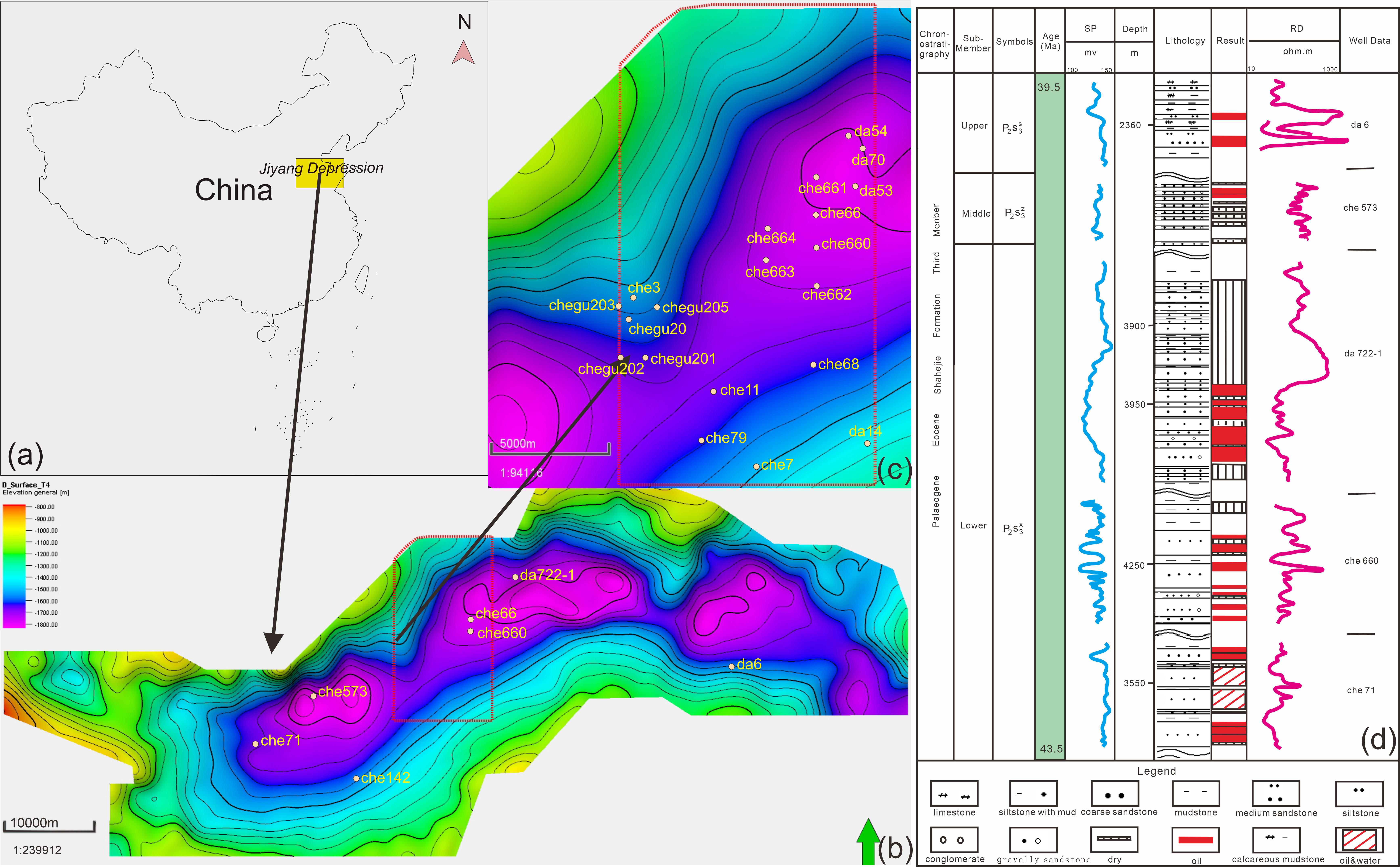
Figure 1 Geographic location of the study area. (A) Map of China. The yellow box is the Jiyang Depression. The Chezhen Depression is a part of the Jiyang Depression. (B) Structural map of the Chezhen Depression. The red dotted box is the location of the Taoerhe Sag. (C) Structural map of the Taoerhe Sag. There are 20 wells on the picture. (D) Stratigraphic and lithologic histogram of the third member of the Shahejie Formation in the Taoerhe Sag.

Structurally, normal faults are developed in the southern part of the depression, and small northwest–southwest-trending faults are locally developed. In general, faults in the depression are not developed, and only faults around the depression are developed (Wang et al., 2007). Stratigraphically, the Cenozoic strata of the Taoerhe Sag include Quaternary, Neogene and Paleogene strata (Li et al., 2018). The target horizon is the third member of the Shahejie Formation of Eocene age. The sediment thickness of the Shahejie Formation is generally more than 200~1000 m (Du et al., 2021). The lithologies of the third member of the Shahejie Formation include dark gray to gray black oil mudstone, oil shale and siltstone, which can be divided into upper (P₂S₃^S), middle (P₂S₃^Z) and lower members (P₂S₃^X) (Zeng et al., 2008; Zhang et al., 2010; Yang et al., 2020; Jfa et al., 2021). In this study, the attribute sensitivity is examined by taking P₂S₃^X as an example. The main lithologies of the lower part of the third member of the Shahejie Formation are mudstone, calcareous oil mudstone and gravelly sandstone; the sediments in the middle part are mainly clay rock, pure mudstone, shale and oil shale; and the sediments in upper part are oil mudstone, oil shale, siltstone and carbonate rock (Zhang et al., 2010; Yang et al., 2020; Jfa et al., 2021). In terms of sedimentation, the gravelly sandstone body in the study area is thin and widely distributed (Zeng et al., 2008; Zhang et al., 2010; Yang et al., 2020; Jfa et al., 2021). The third member of the Shahejie Formation represents the peak of the development of the faulted lake basin. The climate is humid, and gravelly sandstone fans have developed along the lake bank (Yang et al., 2020).

3. Data and methods

3.1. Data

The study area is 212.24 km², covering seismic data, and there are 22 wells in the study area. All data are from the Shengli oil field in China. Seismic data were collected in 2014. The bin grid is 15 m*30 m, the number of coverages is 288, and the horizontal to vertical ratio is 0.54 (Zhao, 2017). The main frequency range of the processed seismic data is 10~35 Hz (Figure 2). The average velocity of the formation below 3000 m in the study area is 3247 m/s (Zhao, 2017), and the seismic resolution is approximately 40 m. The applied logging curves include the natural gamma curve (GR), acoustic time difference curve (AC), density curve (DEN), spontaneous potential curve (SP) and saturated hydrocarbon content (SH). The target stratum of the study is the lower submember of Shahejie Formation 3 (P₂S₃^X).

FIGURE 2

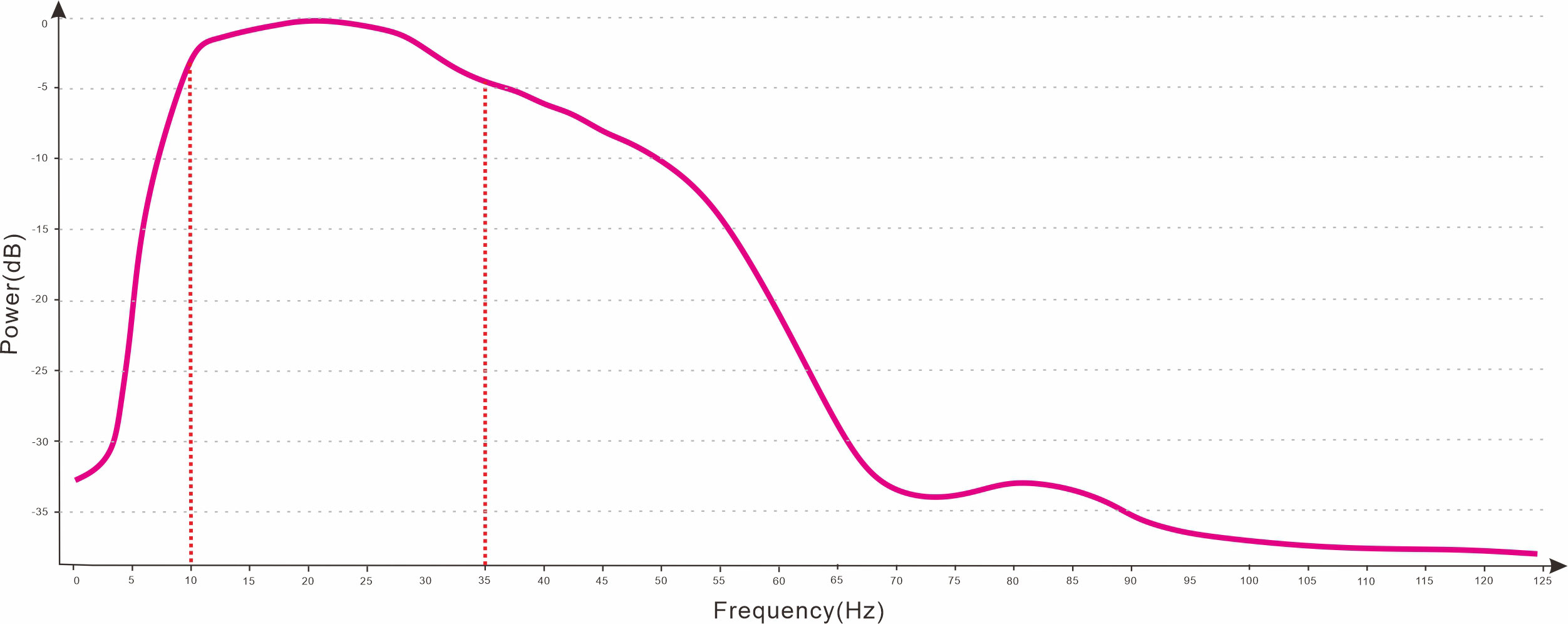
Figure 2 Spectral analysis of the seismic data volume in the Taoerhe Sag. The main frequency range is 10~35 Hz. The high frequency range is 70~85 Hz.

3.2. Methods

As indicated in the introduction, there are two problems that must be solved in this paper. The first problem is the selection of the appropriate seismic attributes. The second problem is the prediction of the thin sandstone of P₂S₃^X in the Taoerhe Sag. The two problems are progressive. Only by selecting the appropriate seismic attributes can we accurately determine the distribution of sandstone in the study area. The research steps can be divided into six steps to solve these two problems (Figure 3). The most critical step is Step 4. We will describe Step 4 in detail.

FIGURE 3

Figure 3 Research flow chart.

Step 4 contains three processes, of which Step a means to extract appropriate seismic attributes. Extracting seismic attributes for the first time requires the “expert optimization method” (Zhao, 2016), that is, extracting seismic attributes according to the experience of geophysical experts. In this paper, sand-body prediction is needed. Therefore, 10 seismic attributes related to sand bodies are extracted based on experience, such as the root mean square amplitude attribute (RMS), instantaneous phase attribute (Phase), and instantaneous frequency attribute (Freq) (Dongjun et al., 2006). However, all of these 10 seismic attributes will not necessarily be used for the final sand-body prediction. These attributes need to be screened, which occurs during Step c, when the seismic attributes are filtered. Step b summarizes the characteristics of sandstone on the logging data and its sensitive parameters. Generally, the characteristics of sandstone based on the loggings are as follows: “bell shaped” or “box shaped”, low GR, and medium - high AC. In addition, when compared with the surrounding rocks, sandstone is mainly characterized by low velocity and low DEN (Collett et al., 2011). In this paper, the crossplot of the logs and rocks are made, and the logging curves with obvious differentiation are selected for further research.

Choosing the appropriate seismic attribute (Step c) is a primary focus of this paper. In the process of seismic reservoir prediction, various seismic attributes related to the reservoir are usually introduced. However, more attributes are not better, as they lead to data redundancy and multiple solutions. Hence, for the specific problem of reservoir prediction, it is very important to select the one attribute that can best express the reservoir characteristics. Seismic attribute optimization (Step c) in this paper includes two secondary steps. The first step is to analyze the correlation between attributes. We next introduce how to analyze the correlation between attributes.

The correlation between two attributes is measured by the correlation coefficient. The correlation coefficient is a digital expression of the degree of correlation between two variables (Barnes, 2007). It is an index used to express the strength of the correlation relationship (Barnes, 2007). The sample correlation coefficient is expressed in R, and the value is generally between -1 and 1 (Barnes, 2007). 1 is the largest positive correlation, 0 is irrelevant, and -1 is the largest negative correlation. In the optimization of seismic attributes, the greater the absolute value of the correlation coefficient between the two is, the higher the degree of correlation; the smaller this value is, the lower the degree of correlation (Barnes, 2007). If the reservoir characteristics expressed by the two seismic attributes are similar, information redundancy and interference occurs in the seismic attribute analysis. Therefore, we can select one of the seismic attributes with a correlation greater than 0.7. The correlation coefficient calculation formula (Barnes, 2007) is as follows:

$\begin{array}{ll}R=\frac{{\sum }^{}\left(X-\overline{X}\right)\left(Y-\overline{Y}\right)}{\sqrt{{\sum }^{}{\left(X-\overline{X}\right)}^2\Sigma {\left(Y-\overline{Y}\right)}^2}}=\frac{l_{xy}}{\sqrt{l_{xx}{l}_{yy}}}& (1)\end{array}$

where X and Y are the values of the two seismic attributes and $\overline{X}$ and $\overline{Y}$ are the average values of X and Y, respectively. The correlation degree is found in Table 1 (Barnes, 2007).

TABLE 1

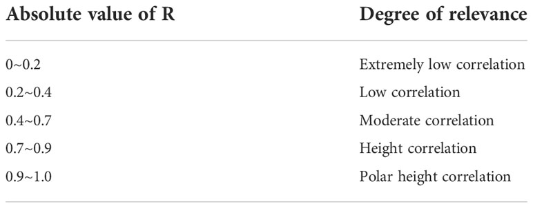
Table 1 Classification standard of correlation degree (Barnes, 2007).

The second step of Step c is to use the seismic attributes selected in the previous step and the logging parameters to implement crossplot analysis; the seismic attributes with good correlation are left. Seismic attributes with good correlation are used for sandstone and reservoir prediction. Among them, the logging parameters sensitive to sandstone are obtained in Step b.

We can find some information by interpreting seismic attribute slices. However, if we confirm that the results are correct, we need to provide more evidence. Hence, we should validate the results via Step 5, including Step d and Step e. For Step d, we use multi-attribute fusion technology to interpret gravelly sandstone. Multi-attribute fusion technology in this paper can be carried out using the following workflow. First, we take a certain attribute slice as the background. Then, we set the transparency of the slice. In addition, we overlay other attribute slices to display more information. This slice is also set to transparency. The transparency is approximately 30% - 50%. Step e involves comparing the results to cores and wells. In this step, we apply genetic algorithm inversion to improve accuracy. When we process genetic algorithm inversion, the input data are issued. Step b indicates which logging parameters can be inversed. We realize genetic algorithm inversion via software named Petrel. Step f in Step 5 refers to the establishment of a comparison chart based on the selected seismic attributes and logging parameters, including seismic attributes, logging curves, and reservoir parameters. The chart can be used for reservoir predictions of other blocks in the work area. This part is explained in the Discussion.

4. Results

4.1. Log analysis (logging characteristics of rocks)

Using the data from 22 wells in the Taoerhe Sag, the lithologic, electrical and logging characteristics of P₂S₃^X are analyzed. There are three main lithologies in P₂S₃^X in the Taoerhe Sag: medium conglomerate, mudstone and calcareous oil mudstone.

Taking Well Che 66 as an example, the depth of calcareous oil mudstone in Figure 4 is 4323.9~4329.0 m, and the thickness is 5.1 m. The GR value of calcareous oil mudstone is 45.4~67.0 API, with an average of 53.0 API. The AC of calcareous oil mudstone is 59.3~67.5 μ S/ft (1 ft = 30.48 cm), with an average of 61.7 μ s/ft. The saturated hydrocarbon content (SH) of calcareous oil mudstone ranges from 4.7 to 24.4, with an average value of 10.1. The resistivity (RD) ranges from 168.7 to 268.6 ohm.m, with an average of 226.9 ohm.m (Table 2).

FIGURE 4

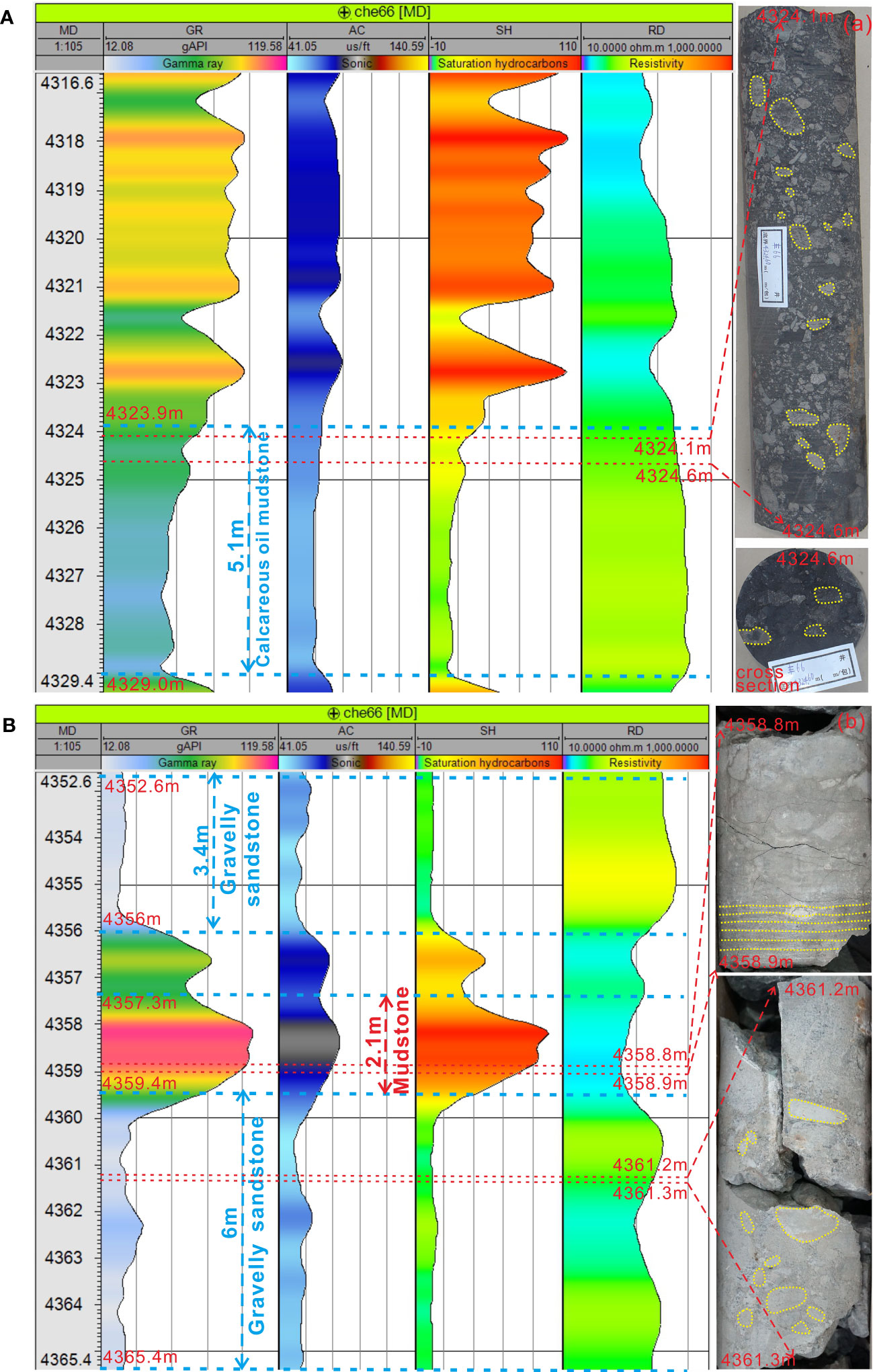
Figure 4 Logging curve characteristics and core characteristics of Well Che 66. (A) Calcareous oil mudstone of Well Che66 is at 4323.9-4329.0 m. The core is calcareous oil mudstone, which is dark. The yellow dotted circle on the core picture is the calcite mud crystal. The core depth is 4324.1-4324.6 m. The core can be related to the logs by depth. (B) Gravelly sandstone of Well Che66 is 4352.6-4356.0 m and 4359.4-4365.4 m. Mudstone of Well Che66 is in 4357.3-4359.4 m. The core depth is 4358.8-4358.9 m (mudstone) and 4361.2-4361.3 m (gravelly sandstone). The core can be related to the logs by depth. The yellow dotted line on the core picture is the horizontal texture during mudstone deposition. The yellow dotted circle on the core picture is mud gravel. We counted the data from 22 well logs and found that the lithologic and electrical characteristics of the lower Sha 3 submember are consistent. Calcareous oil mudstone has medium gamma rays, low acoustic wave time difference, low SH and high RD. Gravelly sandstone is characterized by low GR, low AC, low SH and high RD. Mudstone is characterized by high natural gamma rays, high acoustic transit time, high SH and medium low RD. The crossplot can clarify the differentiation of the above four electrical characteristics for lithology. Taking the well-logging data of P2S3X from Well Che 66 as an example, we completed the production of six kinds of crossplots: GR and AC, GR and SH, GR and RD, AC and SH, AC and RD, and SH and RD. Lithology is used as the intersection background. The crossplot indicates that for the Taoerhe Sag, GR can only be selected if gray oil mudstone and gravelly sandstone are to be distinguished. If we want to distinguish calcareous oil mudstone and mudstone, we can choose GR, AC, or SH. If we want to distinguish mudstone from gravelly sandstone, we can choose GR, AC, or SH. In conclusion, GR can better distinguish lithology.

The thicknesses of the gravelly sandstone in the two sections are 3.4 m and 6 m (Figure 4). The average GR value of gravelly sandstone is 27.1 API. The average value of AC is 57.9 μ s/ft. The average SH is 4.6. The average RD range is 211.3 ohm.m (Table 2).

The depth of the mudstone is 4357.3~4359.4, and the thickness is 2.1 m. The average GR value of mudstone is 87.7 API. The average value of AC is 80.6 μ s/ft. The average SH of gravelly sandstone is 78.1. The average RD range is 74.5 ohm.m (Table 2).

TABLE 2

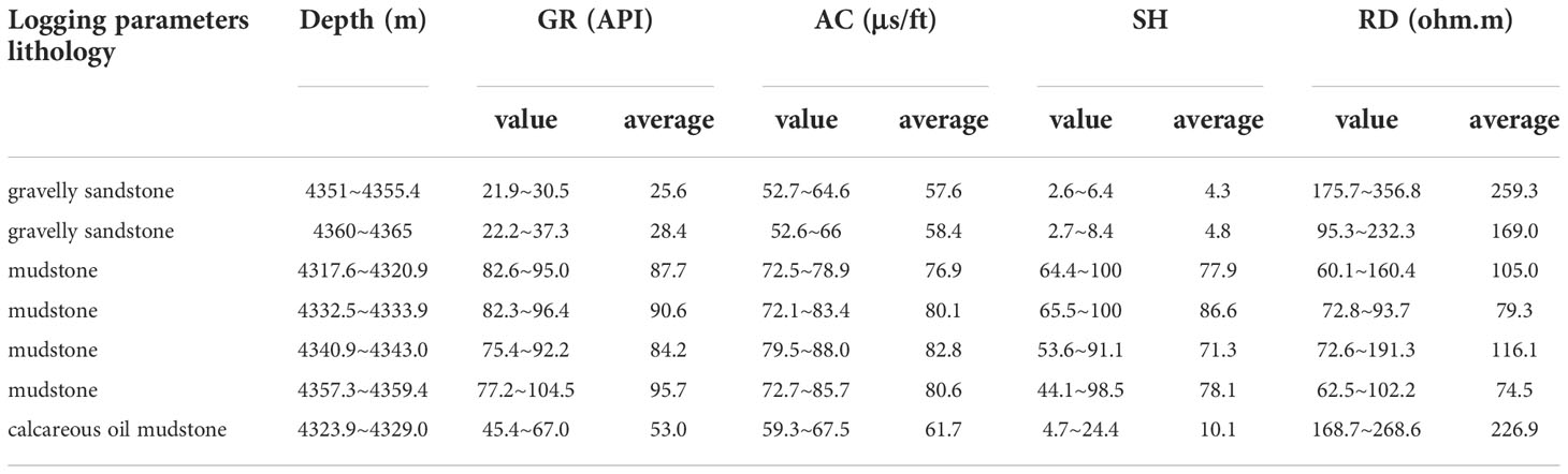
Table 2 Lithology and electricity comparison data of the lower Sha 3 subsection of Well Che 66.

We counted the data from 22 well logs and found that the lithologic and electrical characteristics of the lower Sha 3 submember are consistent. Calcareous oil mudstone has medium gamma rays, low acoustic wave time difference, low SH and high RD. Gravelly sandstone is characterized by low GR, low AC, low SH and high RD. Mudstone is characterized by high natural gamma rays, high acoustic transit time, high SH and medium low RD.

The crossplot can clarify the differentiation of the above four electrical characteristics for lithology. Taking the well-logging data of P₂S₃^X from Well Che 66 as an example, we completed the production of six kinds of crossplots: GR and AC, GR and SH, GR and RD, AC and SH, AC and RD, and SH and RD (Figure 5). Lithology is used as the intersection background. The crossplot indicates that for the Taoerhe Sag, GR can only be selected if gray oil mudstone and gravelly sandstone are to be distinguished. If we want to distinguish calcareous oil mudstone and mudstone, we can choose GR, AC, or SH. If we want to distinguish mudstone from gravelly sandstone, we can choose GR, AC, or SH. In conclusion, GR can better distinguish lithology.

FIGURE 5

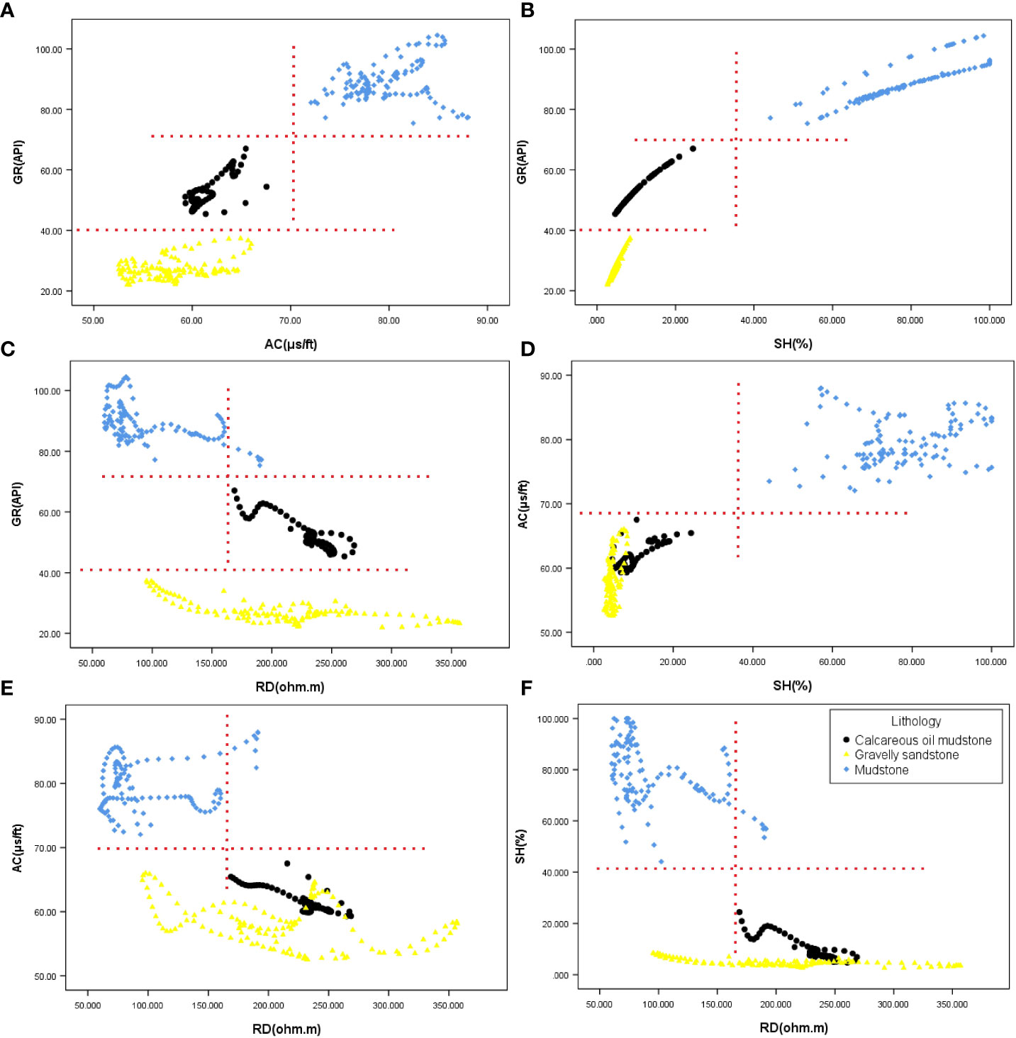
Figure 5 Well Che66 crossplot. (A) GR-AC crossplot; (B) GR-SH crossplot; (C) GR-RD crossplot; (D) AC-SH crossplot; (E) AC-RD crossplot; and (F) SH-RD crossplot. Figures (A–C) show that GR can effectively distinguish mudstone, calcareous oil mudstone and gravelly sandstone. Figure (A), Figure (D) and Figure (E) show that AC can distinguish between mudstone and calcareous oil mudstone and between mudstone and gravelly sandstone, but calcareous oil mudstone and gravelly sandstone overlap greatly in value range. Figure (B), Figure (D) and Figure (F) show that SH can distinguish between mudstone and calcareous oil mudstone and between mudstone and gravelly sandstone, but calcareous oil mudstone and gravelly sandstone overlap greatly in value range. Figure (C), Figure (E) and Figure (F) show that RD can only distinguish mudstone and calcareous oil mudstone. There are overlapping parts between 150 and 200 ohm.m. RD cannot distinguish mudstone from gravelly sandstone. RD cannot distinguish between calcareous oil mudstone and gravelly sandstone.

4.2. Sensitivity analysis of seismic attributes

4.2.1. Correlation analysis of attributes

Three kinds of lithologies are distinguished by seismic attributes: gravelly sandstone, mudstone and calcareous oil mudstone.

Taking the lower segment of Sha 3 as an example, we calculated 10 volume attributes, including amplitude, energy and frequency. These 10 seismic attributes are RMS, sweetness (Sweet), instantaneous bandwidth (BW), 3D curvature (Curv), dominant frequency (Domfreq), approximate polarity (Pol), envelope (Env), phase, reflection intensity (Int), and Freq.

Figure 6 shows the thermodynamic diagram of the correlation coefficient between seismic attributes; for example, the correlation coefficient of RMS and int is 0.99. According to Table 1, the two are highly correlated. One seismic attribute can be obtained by simple mathematical transformation, and the other can be retained. Similarly, referring to Table 1, if the correlation of two attributes reaches 0.7, it is regarded as highly correlated, and only one of them is retained.

FIGURE 6

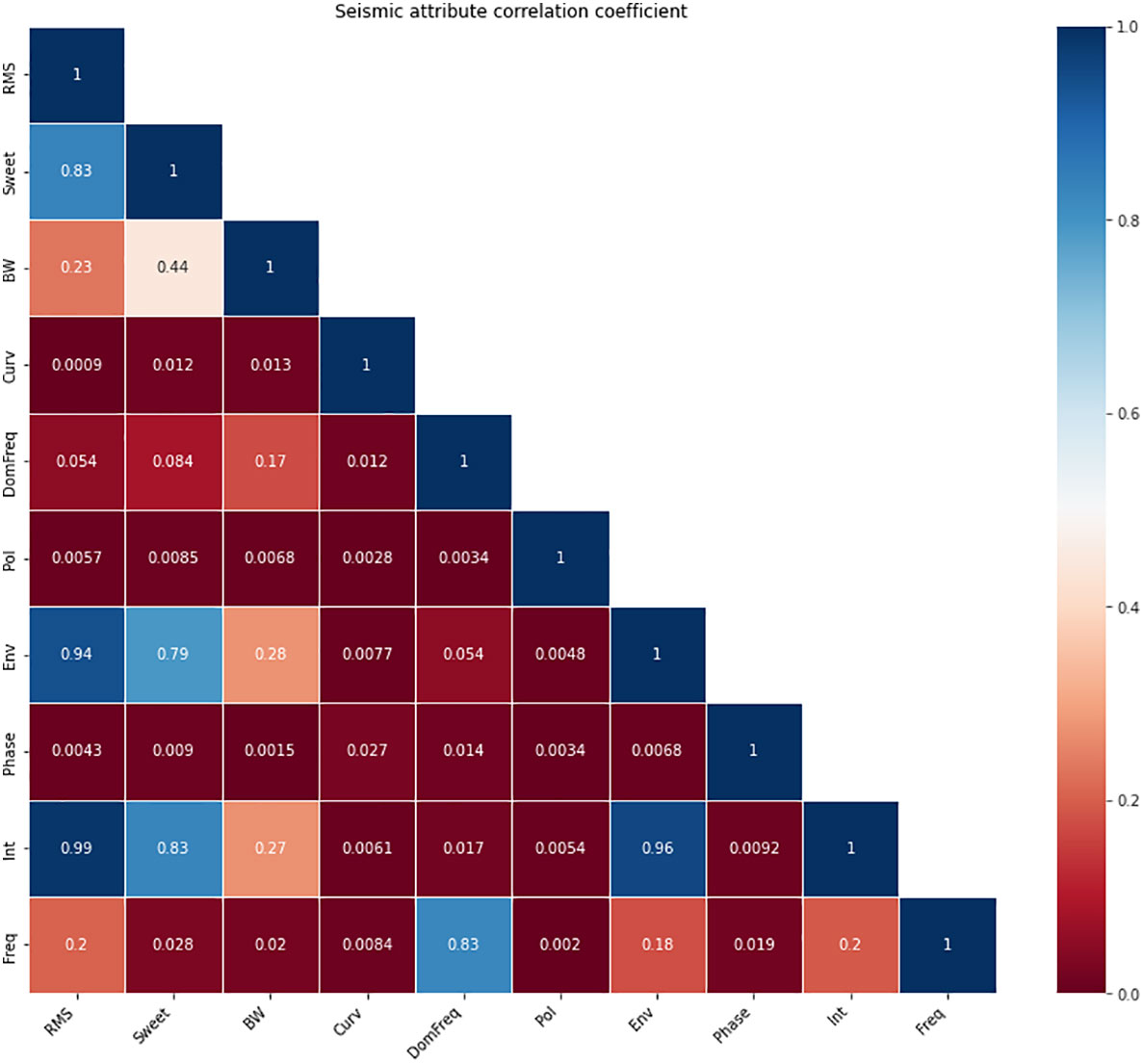
Figure 6 Thermodynamic diagram of seismic attribute correlation. Blue represents height correlation. Red represents low correlation.

According to this method, four seismic attributes are removed, namely, Sweet, Env, Int and DomFreq. Six seismic attributes are retained, namely, RMS, BW, Curv, Pol, Phase and Freq.

4.2.2. GR crossplot of attributes and logging

The six seismic attributes are data bodies. We extracted the seismic attribute data from the well at the same sampling rate (0.076 m) as the logging data. We used Petrel software to perform resampling. To verify the sensitivity of the retained six seismic attributes to lithology, GR data at the same depth and six seismic datasets were selected for intersection analysis (Figure 7). The intersection map shows that except for the pol attribute, the attributes have a certain degree of differentiation for lithology.

FIGURE 7

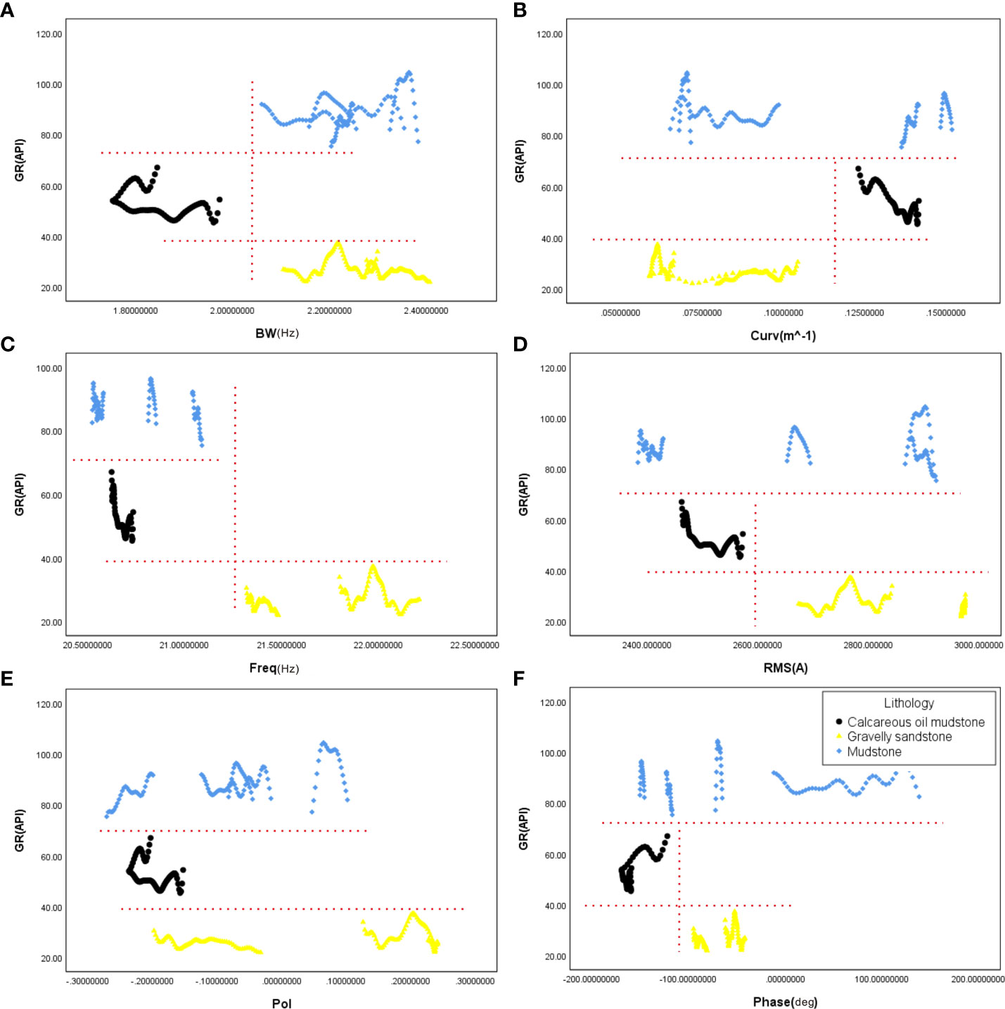
Figure 7 Well Che66 GR-Seismic attribute crossplot. (A) GR-BW crossplot; (B) GR-Curv crossplot; (C) GR-Freq crossplot; (D) GR-RMS crossplot; (E) GR-Pol crossplot; (F) GR-Phase crossplot.

Among them, BW can recognize calcareous oil mudstone. The low value (<2.0 Hz) represents calcareous oil mudstone. The Curv can distinguish between calcareous oil mudstone and gravelly sandstone. Gravelly sandstone has a low value (0.05~0.125 m^ (-1)), and calcareous oil mudstone has a high value (0.125~0.15 m^ (-1)). Freq can recognize gravelly sandstone. High values (>21.5 Hz) represent gravelly sandstone. RMS can distinguish between calcareous oil mudstone and gravelly sandstone. Gravelly sandstone has a high value (>2600a), and calcareous oil mudstone has a low value (<2600a). The Pol attribute cannot distinguish the three lithologies in the study area, and the data coincidence degree is high. Phase can distinguish between calcareous oil mudstone and gravelly sandstone. Gravelly sandstone has a medium-high value (-100~0 deg), and calcareous oil mudstone has a low value (< -100 deg). In summary, high BW, Freq and RMS values represent gravelly sandstone; high BW and RMS values represent mudstone; and low Curv values represent both gravelly sandstone and mudstone. Therefore, when identifying gravelly sandstone, we can compare the above five attributes to obtain its distribution range.

4.2.3. Seismic attribute interpretation

The five attributes, RMS, BW, Curv, Phase and Freq, have a certain lithological differentiation. We first extract five stratigraphic attribute slices of the lower submember of Sha 3. On the RMS slice, the red and yellow areas with values greater than 2600 a (Figure 7D) are divided into gravelly sandstone. In the Curv attribute map, the brown area between 0.05 and ~0.125 m^ (-1) is divided into gravelly sandstone (Figure 7B). In the Freq plan, the high value area (red and yellow) greater than 21.5 Hz (Figure 7C) is divided into gravelly sandstone. In the phase diagram, the yellow and green parts of the -100~0 deg (Figure 7F) area are divided into gravelly sandstone. The TWT map (Figure 8F) shows that there is a river valley in the northern part of the work area, and the river carries sediment into the low-lying area in the middle part of the work area. It is difficult to see obvious valleys in the southern highland area of the work area, and whether there is an alluvial deposit needs to be determined in the discussion part.

FIGURE 8

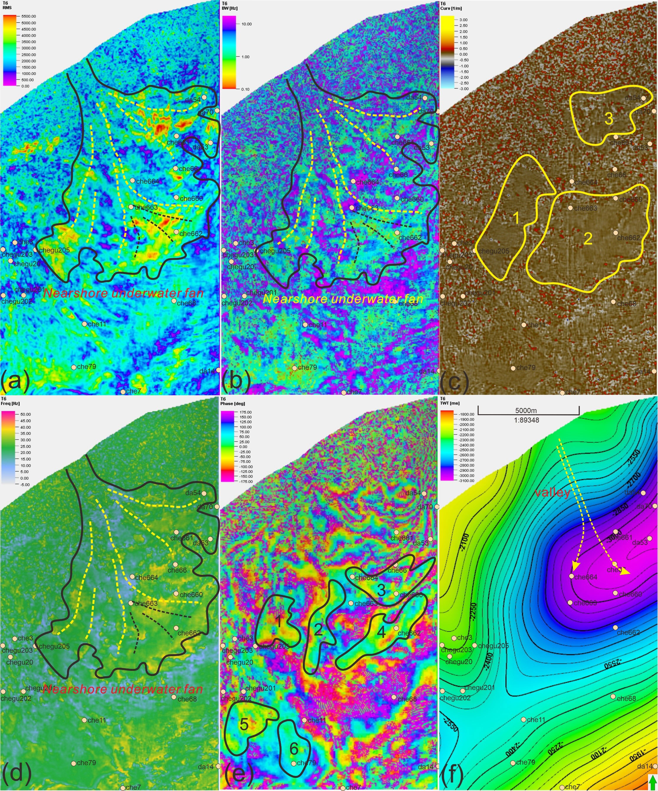
Figure 8 Plan of five attributes of P₂S₃^X. (A) RMS attribute. The black curve is the boundary of the nearshore area under the fan, and the yellow and black dotted lines are river channels. (B) BW attribute. The black curve is the boundary of the nearshore area under the fan, and the yellow and black dotted lines are river channels. (C) Curv attribute. The yellow curve is the boundary of gravelly sandstone deposition. (D) Freq attribute. The black curve is the nearshore boundary under the fan, and the yellow and black dotted lines are river channels. (E) Phase attribute. The black curve is the predicted boundary of gravelly sandstone deposition. (F) The two-way-time contour map. The terrain in the northern area is high, the terrain in the southern area is high, and the terrain in the middle area is low. Therefore, there is a depression in the middle. Sediments were transported from high to low along the river channel and deposited on the slope zone and lake bottom.

Comparing the reflection results of the lithology on the five attribute maps, combined with the structural map of the study area, we believe that the nearshore underground fan (Figures 8A, B, D) was deposited in the northern part of the study area. The RMS, BW and Freq attributes can clearly distinguish the boundary of the fan. Gravelly sandstone is mainly distributed in the middle part of the fan and deep lake bottom of the slope zone, with a total area of approximately 39.5 km². Curv and Phase can only recognize gravelly sandstone, but the sedimentary boundary of the fan is not obvious. In the Curv attribute graph, three gravelly sandstone blocks can be depicted. Units 1~3 (Figure 8C) are within the range of the nearshore underwater fan. Six gravelly sandstone blocks are identified in the phase attribute map. However, after comparison with the Freq attribute map, blocks 5 and 6 (Figure 8E) are ultimately not recognized as gravelly sandstone.

5. Discussion

To verify the correctness of the above attribute analysis results, we use multi-attribute fusion technology and genetic algorithm inversion.

When we use a single attribute to identify sandstone, there will be multiple results. In this way, multi -attribute fusion technology should be considered. In recent years, scholars have made significant progress in exploring multi-attribute fusion technologies or methods (Mcardle and Ackers, 2012; Maleki et al., 2019). RGB color blending is one method of multi-attribute fusion technology, which has been used to show subtle lithological changes (Mcardle and Ackers, 2012). In this paper, fusion is easy to achieve. We overlay two slices, and we set different transparencies to show more information from the two slices (Figures 9A, B).

The genetic algorithm (GA) was proposed by Professor J.H. Holland at the University of Michigan (Holland, 1992). GA is a randomized search method based on the evolutionary laws of the biological world (Holland, 1992). This algorithm can solve the optimal value (Holland, 1992). Genetic algorithm inversion has frequently been applied to deep-sea basin reservoir prediction. Chinese scholars took a central paddy sandstone reservoir in a deep-water area as an example and predicted the distribution characteristics of favorable reservoirs using the GA method, which greatly reduced the exploration risk (Huang, A. M., Li, L., 2011). GA can also be applied to calculate rock compressive strength (Xiong et al., 2021).

GR data and original seismic data are used as input for the genetic algorithm. The inverted data volume is then obtained. The GR curve and AC curve are projected on the seismic profile after inversion, and the coincidence between the two curves and the seismic inversion volume data is counted (Figure 9C). Both GR and AC of gravelly sandstone are low values. The GR and AC data from 22 well logs in the study area are compared. The coincidence between the borehole data and the inversion profile is more than 90%, thus, the reliability of the inversion body is high.

FIGURE 9

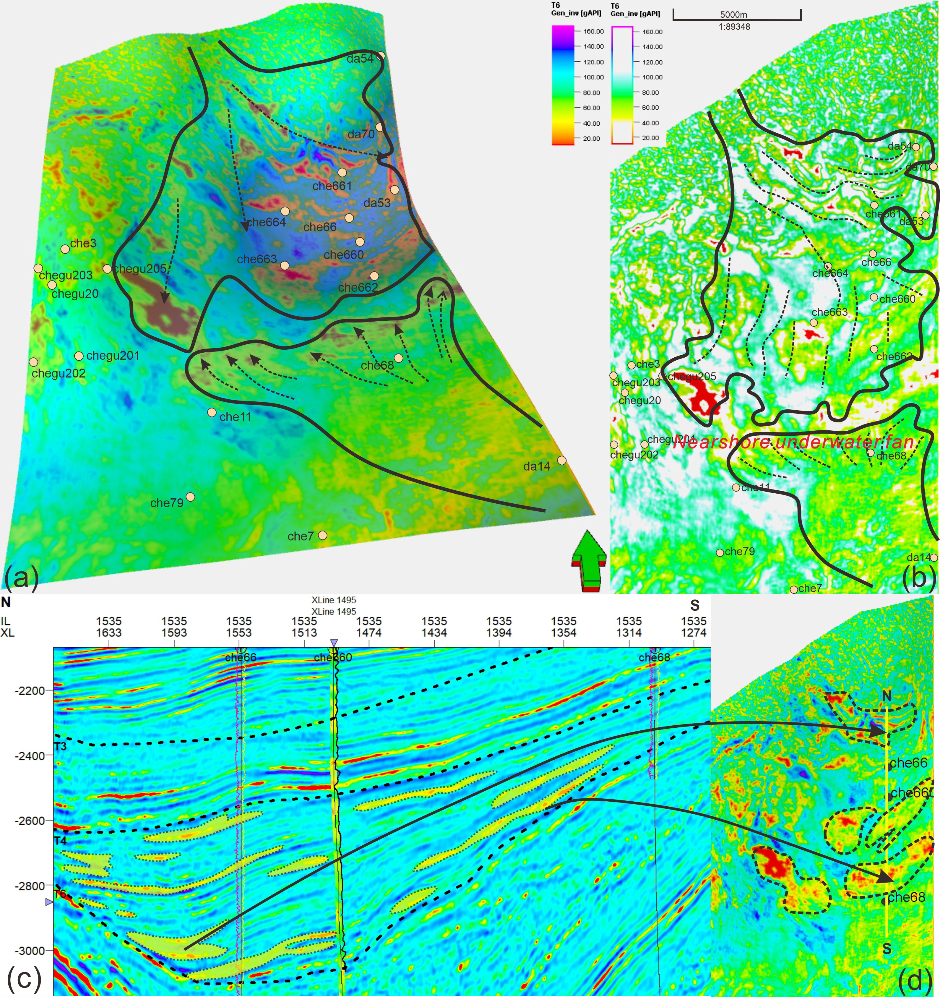
Figure 9 Inversion stratigraphic slice and profile of P₂S₃^X. (A) Multiattribute fusion technology - superposition map from GR genetic inversion stratigraphic slice and structural map. The black curve represents a fan. Red and yellow represent GR low values, representing gravelly sandstone. Based on the 3D structural map, it is inferred that two fans were developed in this area: one was from the northern mountainous area, and the other was from the southern mountainous area. (B) GR genetic inversion stratigraphic slices after filtering high and very low values. This figure can depict the fan more clearly. The black curve represents a fan. (C) GR genetic inversion profile. T3 is the top of P₂S₃^S. T4 is the top of P₂S₃^Z. T6 is the bottom of P₂S₃^X. The red curve on the left side of Well che66 is the GR curve (the curve protruding to the right indicates a low GR value), and the yellow curve on the right is the AC curve (the curve protruding to the left indicates a low AC value). The middle axis of the che660 well is the extracted above-well Freq attribute, and red and yellow are high values, representing gravelly sandstone. The black curve on the right is the AC curve (the curve highlighted to the left indicates that the AC value is low). The red curve on the left of Well che68 is the GR curve (the curve protruding to the right indicates a low GR value), and the yellow curve on the right is the AC curve (the curve protruding to the left indicates a low AC value). The yellow area circled by the dotted point is gravelly sandstone delineated from the profile. (D) Unfiltered GR genetic inversion stratigraphic slices with high and very low values. The black dotted line is the distribution range of gravelly sandstone finally delineated on the plane. The yellow straight line is the location of Section (C).

For the nearshore underwater fan in the study area, the distribution range of gravelly sandstone shown by the stratigraphic inversion volume slice of P₂S₃^X is consistent with the conclusion obtained in Figure 8. The superimposed map of stratigraphic slices and structures (Figure 9A) clearly shows that a part of the nearshore underwater fan is also developed in the southern part of the work area. Due to the scope limitation of the work area, we cannot examine all sedimentary boundaries of the fan. Obviously, a relatively thick gravelly sandstone was deposited on the front edge of the fan. After adding this fan, the total distribution area of gravelly sandstone in the study area is approximately 57.9 km² (Figure 9D).

In addition to the Taoerhe Sag, there are also three subdepressions: the Dawangzhuang Sag, Chexi Sag and Guojuzi Sag in the Chezhen Depression. The attribute optimization scheme discussed in this paper can be extended to these three depressions to depict the distribution range of gravelly sandstone or other rocks. We will explore this engineering problem in the future.

6. Conclusion

In this paper, through the methods of sensitive attribute optimization and attribute fusion, three logging attributes and five seismic attributes that can distinguish gravelly sandstone are selected in the Taoerhe Sag. The prediction results of seismic attributes are explained. Finally, the correctness of the interpretation results is evaluated through GR genetic inversion data volume, and a set of gravelly sandstone prediction parameters and methods suitable for the Taoerhe Sag are formed. The main conclusions are as follows. The results of log analysis show that for the Taoerhe Sag, GR can only be selected if calcareous oil mudstone and gravelly sandstone are distinguishable. If we want to distinguish calcareous oil mudstone and mudstone, we can choose GR, AC, or SH. If we want to distinguish mudstone from gravelly sandstone, we can choose GR, AC, or SH. GR has the most obvious distinction for lithology. The sensitivity analysis results of the seismic attributes show that the five primary attributes are RMS, BW, Curv, Phase and Freq, which have a certain degree of lithological differentiation in the study area. The results of seismic attribute interpretation show that there is a nearshore underwater fan in the northern and southern parts of the study area, and gravelly sandstone is distributed in the slope zone and the lake bottom. The distribution range of gravelly sandstone in the study area is 57.9 km².

The research methods of logging attribute optimization, seismic attribute sensitivity analysis, genetic algorithm inversion, and quality control can both identify lithologic characteristics in the deep Earth and provide a basis for planning drilling locations. In future research work, this method can be applied to other deep-sea depressions.

Data availability statement

The original contributions presented in the study are included in the article/supplementary material. Further inquiries can be directed to the corresponding author.

Author contributions

Conceptualization, JZ and JM. Methodology, NL. Software, NL and MD. Validation, NL and XL. Formal analysis, NL and TC. Investigation, XL and LW. Resources, JZ and JM. Data curation, NL. Writing-original draft preparation, NL and XL. Writing-review and editing, JZ and JM. Visualization, XL. Supervision, JZ and JM. Project administration, JZ. Funding acquisition, JZ. All authors contributed to the article and approved the submitted version.

Funding

This research is supported by the National Study Abroad Fund and the Scientific Research Fund Project of Education Department of Liaoning Province, grant number L2020008.

Acknowledgments

We thank Shengli Oilfield for providing capital, logging, borehole, seismic data and software. SPSS software was provided by BNU. We also thank the National Study Abroad Fund Committee China and Scientific Research Fund Project of Education Department of Liaoning Province (L2020008) for providing funding.

Conflict of interest

Author MD was employed by Shengli Oilfield Dongsheng Jinggong Petroleum Development Group Co., Ltd.

The remaining authors declare that the research was conducted in the absence of any commercial or financial relationships that could be construed as a potential conflict of interest.

Publisher’s note

All claims expressed in this article are solely those of the authors and do not necessarily represent those of their affiliated organizations, or those of the publisher, the editors and the reviewers. Any product that may be evaluated in this article, or claim that may be made by its manufacturer, is not guaranteed or endorsed by the publisher.

References

Abdullatif O. M., Sitouah M. (2011). “Reservoir porosity and permeability prediction from petrographic data using artificial neural network: a case study from Saudi Arabia,” in 9th middle east geosciences conference geo 2010. Geoarabia, European Association of Geoscientists & Engineers. doi: 10.3997/2214-4609-pdb.248.103

CrossRef Full Text | Google Scholar

Baouche R., Nabawy B. S. (2021). Permeability prediction in argillaceous sandstone reservoirs using fuzzy logic analysis: a case study of triassic sequences, southern hassi r’mel gas field, algeria. J. Afr. Earth Sci. 173, 104049. doi: 10.1016/j.jafrearsci.2020.104049

CrossRef Full Text | Google Scholar

Barnes A. E. (2007). Redundant and useless seismic attributes. Geophysics 72 (3), 978. doi: 10.1190/1.2716717

CrossRef Full Text | Google Scholar

Collett T. S., Lewis R. E., Winters W. J., Lee M. W., Rose K. K., Boswell R. M. (2011). Downhole well log and core montages from the mount Elbert gas hydrate stratigraphic test well, Alaska north slope. Mar. Petroleum Geology 28 (2), 561–577. doi: 10.1016/j.marpetgeo.2010.03.016

CrossRef Full Text | Google Scholar

Dongjun T., Fu E., Sullivan C., Kurt J M. (2006). Rock property- and seismic-attribute analysis of a chert reservoir in the devonian thirty-one formation, west texas, U.S.A. Geophysics 71 (5), B151–B158. doi: 10.1190/1.2335636

CrossRef Full Text | Google Scholar

Du P., Cai J., Liu Q., Zhang X., Wang J. (2021). A comparative study of source rocks and soluble organic matter of four sags in the jiyang depression, bohai bay basin, ne china. J. Asian Earth Sci. 216, 104822. doi: 10.1016/j.jseaes.2021.104822

CrossRef Full Text | Google Scholar

Edwards M. B. (1994). “Enhancing sandstone reservoir prediction by mapping erosion surfaces, lower miocene deltas, southwest louisiana, gulf coast basin,” in Gulf coast association of geological societies transactions, (Austin, TX, United States: OSTI.GOV) vol. 44. , 205–215. Available at: https://archives.datapages.com/data/gcags/data/044/044001/0205.htm#purchaseoptions.

Google Scholar

Ferguson R. J., Margrave G. F. (1996). A simple algorithm for band-limited impedance inversion. CREWES Res. Rep. 8, 1–11. doi: 10.1.1.578.3383

Google Scholar

Fouad, Khaled, Jennette, David C., Soto-Cuervo, Arturo (2002). “Fluid prediction from 3-d seismic data in deepwater sandstone reservoirs: applications from cocuite gas field, veracruz basin, southeastern mexico,” in Gulf Coast Association of Geological Societies Transactions, vol. 52. , 291–300. Available at: https://archives.datapages.com/data/gcags/data/052/052001/0291.htm.

Google Scholar

Galloway W. E. (2012). Clastic depositional systems and sequences: applications to reservoir prediction, delineation, and characterization. Leading Edge 17 (2), 173–180. doi: 10.1190/1.1437934

CrossRef Full Text | Google Scholar

Ge J., Zhu X., Jones B. G., Zhang Y., Huang H., Shu Y. (2018). Facies delineation and sandstone prediction using seismic sedimentology and seismic inversion in the eocene huizhou depression, pearl river mouth basin, china. Interpretation, 6 (2), 1–51. doi: 10.1190/int-2017-0155.1

CrossRef Full Text | Google Scholar

Holland J. H. (1975). Adaption in natural and adaptive systems. Appl. Radiat. isotopes. doi: 10.1021/ja211220r

CrossRef Full Text | Google Scholar

Holland J. H. (1992). Adaption in natural and adaptive systems. (MIT Press, Massachusetts), 35–66. doi: 10.7551/mitpress/1090.001.0001

CrossRef Full Text | Google Scholar

Jfa B., Jq A., Hw C., Qr A. (2021). Quantitative prediction of multiperiod fracture distributions in the cambrian-ordovician buried hill within the futai oilfield, jiyang depression, east china. J. Struct. Geology 148, 104359. doi: 10.1016/j.jsg.2021.104359

CrossRef Full Text | Google Scholar

Johannessen E. R., Mjs R., Renshaw D., Dalland A., Jacobsen T. (1995). Northern limit of the "brent delta" at the tampen spur -a sequence stratigraphic approach for sandstone prediction. Norwegian Petroleum Society Special Publications 5, 213–223, 229–256. doi: 10.1016/S0928-8937(06)80070-6

CrossRef Full Text | Google Scholar

Lamy P., Swaby P. A., Rowbotham P. S., Dubrule O., Haas A. (1999). From seismic to reservoir properties with geostatistical inversion. Spe Reservoir Eval. Eng. 2 (4), 334–340. doi: 10.2118/57476-PA

CrossRef Full Text | Google Scholar

Li J., Ma Y., Huang K., Zhang Y., Wang W., Liu J., et al. (2018). Quantitative characterization of organic acid generation, decarboxylation, and dissolution in a shale reservoir and the corresponding applications–a case study of the bohai bay basin. Fuel 214 (FEB.15), 538–545. doi: 10.1016/j.fuel.2017.11.034

CrossRef Full Text | Google Scholar

Maleki M., Davolio A., Denis J. S. (2019). Quantitative integration of 3d and 4d seismic impedance into reservoir simulation model updating in the norne field. Geophysical Prospecting 67 (1), 167–187. doi: 10.1111/1365-2478.12717

CrossRef Full Text | Google Scholar

Mcardle N. J., Ackers M. A. (2012). Understanding seismic thin-bed responses using frequency decomposition and rgb blending. First Break 30, (1956). doi: 10.3997/1365-2397.2012022

CrossRef Full Text | Google Scholar

Nisar A., Wiktor W. W., Dario G. (2022). Constrained non-linear AVO inversion based on the adjoint-state optimization. Comput. Geosci. 168, 105214. doi: 10.1016/j.cageo.2022.105214

CrossRef Full Text | Google Scholar

Primmer T. J., Cade C. A., Evans J., Gluyas J. G., Mark S. H., Norman H. O., et al. (1997). Global patterns in sandstone diagenesis: their application to reservoir quality prediction for petroleum exploration. Am Assoc. Petrol. Geol. 69, 61–78. doi: 10.1306/M69613C5

CrossRef Full Text | Google Scholar

Simon M., Lutz R., Dieter F., Christoph G., Jutta W. (2018). Shallow gas accumulations in the German north Sea. Mar. Petroleum Geology 91, 139–151. doi: 10.1016/j.marpetgeo.2017.12.016

CrossRef Full Text | Google Scholar

Wang R. L., Sun J., Li J. G. (2007). The recognition on oil-gas reservoir of glutinite body of sha 3 sub-inter of CH 66 block in taorhe shallow depression. Mud Logging Eng. 02, 62–68+78.

Google Scholar

Xiong X., Gao F., Zhou K., Gao Y., Yang C. (2021). Intelligent prediction model of the triaxial compressive strength of rock subjected to freeze-thaw cycles based on a genetic algorithm and artificial neural network. Geofluids 2021 (7), 1–12. doi: 10.1155/2021/1250083

CrossRef Full Text | Google Scholar

Xu K., Greenhalgh S. (2010). Ore-body imaging by crosswell seismic waveform inversion: a case study from kambalda, western australia. J. Appl. Geophysics 70 (1), 38–45. doi: 10.1016/j.jappgeo.2009.11.001

CrossRef Full Text | Google Scholar

Yang T., Cao Y., Friis H., Liu K., Zhang S. (2020). Diagenesis and reservoir quality of lacustrine deep-water gravity-flow sandstones in the eocene shahejie formation in the dongying sag, jiyang depression, eastern China. AAPG Bull. 104 (5), 1045–1073. doi: 10.1306/1016191619917211

CrossRef Full Text | Google Scholar

Zeng Z., Fang H., Song G., Sui F., et al. (2010). Palaeo-formation pressure evolution and episodic hydrocarbon accumulation in tao’erhe depression, chezhen sag. Oil Gas Geology 31 (2), 193–197+205. doi: 10.11743/ogg20100209

CrossRef Full Text | Google Scholar

Zeng H. L., Robert G., Loucks L., Frank B. (2007). Mapping sediment dispersal patterns and associated systems tracts in fourth- and fifth-order sequences using seismic sedimentology: example from corpus christi bay, Texas. AAPG Bull. 91 (7), 981–1003. doi: 10.1306/02060706048

CrossRef Full Text | Google Scholar

Zeng Z. P., Song G. Q., Liu K. Y. (2008). Overpressure mechanisms in taoerhe sag of chezhen depression. Bull. Geological Sci. Technol. 06, 71–75.

Google Scholar

Zhang Y., Xia B., Wan N., Wan Z., Shi Q., Song C. (2010). Tectonic controls on the hydrocarbon accumulations in the chexi sag. Geotectonica Et Metallogenia 34 (4), 593–598. doi: 10.1145/1836845.1836984

CrossRef Full Text | Google Scholar

Zhang J. H., Zhen L., Zhu B. H., Feng D. Y., Zhang M. Z., Zhang X. F. (2011). Fluvial reservoir characterization and identification: a case study from laohekou oilfield. Appl. Geophysics 8 (003), 181–188. doi: 10.1007/s11770-011-0288-y

CrossRef Full Text | Google Scholar

Zhao W. P. (2016). The application of well-seismic joint attribute analysis technique to the prediction of deep-water turbidite sand reservoir. J. Eng. Geophysics 13 (02), 213–220.

Google Scholar

Zhao Z. H. (2017). Study on high-precision seismic acquisition method in gentle slope zone of chezhen depression (Qingdao: China University of Petroleum (East China). doi: 10.27644/d.cnki.gsydu.2017.000184

CrossRef Full Text | Google Scholar

Appendix

Root mean square amplitude computes RMS on instantaneous trace samples over a specified window (default 9 samples).

Sweetness is defined as envelope/sqrt (Instantaneous frequency). For numerical reasons, a lower threshold of frequency is set at 1 Hz.

The instantaneous bandwidth is the absolute value of the time derivative of the envelope.

3D curvature is the curvature of the reflectors/seismic structure of a volume.

The dominant frequency is from the measure of the hypotenuse between the instantaneous frequency and instantaneous bandwidth.

Apparent polarity is the polarity of the instantaneous phase. It is calculated at the local amplitude extrema.

The envelope is also known as the instantaneous amplitude, magnitude or reflection strength. It is the instantaneous magnitude of the analytic signal (the complex trace), independent of phase: env = sqrt(sqr(f)+sqr(g)).

The instantaneous phase is an argument of the analytic signal. phase=arctan(g/f), where f(t) is the real part and g(t) is the imaginary.

Reflection intensity integrates the instantaneous amplitude along the trace (using the trapezoidal rule).

Instantaneous frequency is the time derivative of phase (d(phase)/dt). The time derivative of the instantaneous phase is often referred to as ‘phase acceleration’.