Analysis and prediction of marine heatwaves in the Western North Pacific and Chinese coastal region

1 Introduction

The global ocean has significantly warmed in the past century, profoundly impacting marine ecosystems. More than 90% of heat increase due to global warming is absorbed by the ocean’s upper layer (Pörtner et al., 2019). The long-term continuous warming of the ocean resulted in an increase in the frequency of discrete extreme regional oceanic warming events (i.e., marine heatwaves, MHWs). MHWs occur in almost every area of the world’s oceans (Scannell et al., 2016; Han et al., 2022; Yao et al., 2022), such as in the Pacific Ocean (Capotondi et al., 2022; Holbrook et al., 2022), the tropical Indian Ocean (Zhang et al., 2021), the Arctic (Huang et al., 2021), the Mediterranean Sea (Black et al., 2004; Olita et al., 2007), the South China Sea (Yao and Wang, 2021; Liu et al., 2022; Wang et al., 2022a; Wang et al., 2022b), the Japan/East Sea (Wang et al., 2022c), the Mozambique Channel (Mawren et al., 2021), the Oyashio Region (Miyama et al., 2021), and China’s adjacent offshore waters (Gao et al., 2020; Yao et al., 2020).

Based on the OISSTV2 data, the frequency and duration of global MHWs have increased by 34 and 17%, respectively, in the past century (Oliver et al., 2018). From 1982 to 2016, the average MHW days increased by 30 days/year. It is important to note that the changing trend correlates well with the rise in the average sea surface temperature (SST). This correction indicates that MHWs will occur more frequently under continuous global warming. The multi-model ensemble average results based on the Coupled Model Intercomparison Project Phase 5/6 (CMIP5/6) show that most of the world’s oceans will reach the annual sustainable MHW state by the end of this century (Oliver et al., 2019).

MHW events are expected to increase in frequency and intensity, pushing marine organisms and ecosystems to the limit of their resilience or even higher, which may lead to irreversible damage (Frölicher et al., 2018; Garrabou et al., 2022). MHWs can damage marine biodiversity (Bond et al., 2015; Hughes et al., 2017; Jones et al., 2018; Straub et al., 2019; Thomsen et al., 2019; Morrison et al., 2020; Yao and Wang, 2022), the world fisheries, and aquaculture industries (Mills et al., 2013; Cavole et al., 2016; Chandrapavan et al., 2019) by leading to large-scale coral bleaching and reduced kelp forests and seagrass meadows (Holbrook et al., 2020; Feng et al., 2022). According to field surveys and satellite images, MHWs in 2010/11 damaged 36% of the seagrass meadow in Shark Bay (Arias-Ortiz et al., 2018). Wernberg et al. (2013) pointed out that extreme MHWs have forced coastal forests to shrink by 100 km, and temperate species have been replaced by seaweeds, invertebrates, corals, and fishes unique to subtropical and tropical waters. This propagation of the whole community has fundamentally changed the critical ecological processes, resulting in irreversible changes in coastal forests. When seawater temperature during MHWs exceeds the thermal tolerance limit of marine species, it results in the large-scale death of fish and invertebrates, especially those species distributed in shallow water or low-tide areas.

MHWs also promote the development of harmful algal blooms (HABs), negatively impacting food security, tourism, the local economy and human health. Large-scale HABs cause environmental problems such as fish death and environmental degradation due to high biomass. Consumption of HAB-contaminated fish by humans can lead to various diseases. The adverse effects of MHWs on marine ecosystems are long-lasting. Caputi et al. (2019) found that after seven years, only some ecosystems in Western Australia showed promising recovery due to the impact of the extreme MHW in 2011. During this MHW event that affected 2,000 km of the Australian Midwest coast, the SST was 2 ~ 5°C higher than the climatological average temperature (Caputi et al., 2016).

The generation mechanism of MHWs is very complex, not only with local dependence but also related to large-scale atmospheric and oceanic background fields (e.g., Misra et al., 2021; Hu et al., 2021). Specific generation mechanisms include the followings.

1.1 Local oceanic current anomalies

An MHW with the longest duration (251 days) and highest intensity (2.9°C) on record occurred in the Tasman Sea in 2015/16. The anomalous heat concentration associated with the southward-flowing East Australian Current was the main reason for this MHW event (Oliver et al., 2017). Similarly, the weakening of cold advection in the South China Sea is considered the inducing factor of MHW in 2021 (Yao and Wang, 2021).

1.2 Compound effect of extreme La Niña events, oceanic current anomalies and air-sea heat flux anomalies

Pearce and Feng (2013) pointed out that the MHW along the western coast of Australia during the austral summer of 2010/11 was a combination of a near-record more significant La Niña event, a record strength Leeuwin Current, and an anomalously high air-sea heat flux into the ocean. This MHW event in February 2011 led to an anomalous SST peak in the coastal and offshore areas (more than 200 km) from Ningaloo (22°S) to Cape Leeuwin (34°S), which was 3°C higher than the long-term monthly average.

1.3 El Niño teleconnections

Combining observation results with climate model simulations, it is reported that the teleconnections between the North Pacific and the weak 2014/15 El Niño induced the MHW event in the Northeast Pacific during the winters of 2013/14 and 2014/15 (Di Lorenzo and Mantua, 2016). The El Niño event also drives the MHWs in tropical Australia during 1997/98 and 2015/16 (Zhang et al., 2017; Benthuysen et al., 2018).

Besides, the weakening of the wind field (Garrabou et al., 2009), air-sea heat flux and heat advection anomaly (Xu et al., 2018), and ENSO events (Holbrook et al., 2019) could also induce MHWs. In conclusion, the MHWs generation mechanism is very complex, and its impact area and occurrence frequency are getting broader and higher.

Previous studies based on CMIP5 models indicate that the increase in MHWs intensity and days is expected to accelerate. However, the inadequacy of the CMIP5 and the regional dependence of MHWs require further study with improved numerical models. Hamed et al. (2022) pointed out that most climate variables simulated in CMIP6 are less biased than in CMIP5. Preliminary studies show that the WNPCC region is one of the regions most affected by MHWs (Li et al., 2019). Since 1970, the SST rise in this region has been higher than the global average in the same period. Under different projection scenarios, the WNPCC area may become one of the areas with the highest global ocean temperature rise. During the stagnation period of global warming, the frequency and intensity of MHW in the WNPCC area did not decrease, but it was more frequent and lasted longer than in other regions. Oliver et al. (2018) pointed out that the frequency and average intensity of MHW in the Northwest Pacific from 2000 to 2016 increased by 1 ~ 4 times/year and 1 ~ 2.5°C, respectively, compared with 1982 ~ 1998.

In summary, MHWs impact is getting increasingly severe, and the resulting loss is getting larger. For proactive marine management, it is essential to understand how MHWs will change (Yao et al., 2022). Operators in the coastal and marine sectors can use MHW events projections for better planning. These sectors include subsistence and commercial fishing, diving, aquaculture, fisheries management, tourism, conservation management, and policy development. It is urgent to discuss and analyze MHWs in the WNPCC area.

The rest of this study is organized as follows. Section 2 introduces the data employed in this study, the definition of MHW, MHWs characteristics, and seven parameters used in model evaluation. Section 3 presents the basic characteristics of MHWs in the WNPCC area during the historical period (1982 ~ 2014). The projection characteristics (2015 ~ 2100) under SSP1-2.6, 2-4.5 and 5-8.5 are illustrated in Section 4. In Section 5, we discuss the seasonal variation of MHWs characteristics, the impact of different climate thresholds and the subsurface MHWs. The conclusions are given in Section 6.

2 Data and methods

2.1 OISSTV2

This study employs the Optimal Interpolated Sea Surface Temperature version 2 (OISSTV2) data to evaluate the ability of CMIP6 global climate models (GCMs) to capture MHWs in the historical period (1982 ~ 2014). It is the product of data synthesis and interpolation of multiple observation platforms (satellites, ships, buoys, and Argo profiles) into a regular global grid, with a spatial resolution of 0.25° by 0.25° and a daily time resolution. Many researchers have used this data to study MHWs or SST variation (Yan et al., 2020; Jacox et al., 2022; Noh et al., 2022; Zhang et al., 2022). For more details about this dataset, please refer to Reynolds et al. (2007).

2.2 CMIP6

CMIP6 is the latest global climate simulation that provides information for the sixth assessment report of the Intergovernmental Panel on Climate Change (O'Neill et al., 2016). This dataset has the most significant number of participation GCMs, a well-designed array of scientific experiments, and an enormous amount of simulation data during the 20 years of implementation of the plan (Eyring et al., 2016; Wei et al., 2021; Kajtar et al., 2022; Scafetta, 2022). The CMIP6 historical simulation experiment was completed at the end of 2014, and future scenarios were gradually added later. A new set of emission scenarios driven by different socio-economic models, the Shared Socioeconomic Pathways (SSP), developed in CMIP6, replaces the four Representative Concentration Pathways (RCP) in CMIP5 and dramatically improves the inadequacy of RCP scenarios. Climate prediction under different SSP scenarios reflects different carbon emission policies’ climate impacts and socio-economic risks.

This study extracts MHW characteristics from CMIP6 data during the historical period in the WNPCC area and compares them with the results obtained from OISSTV2 data to evaluate the ability of 19 CMIP6 models (Table 1) to simulate MHWs. Top-performing models are then selected to analyze the projected changes in MHWs characteristics and trends. This study considers three emission scenarios for projection studies: SSP1-2.6, 2-4.5, and 5-8.5. They represent a low, medium, and high emission scenario, where solar radiation will increase by 2.6, 4.5, and 5.8 W/m² by the end of 21 century. To compare the difference in MHWs characteristics between the OISSTV2 and CMIP6 model data, all the data are interpolated to a 1° by 1° resolution grid. All analyses are conducted using the interpolated data.

TABLE 1

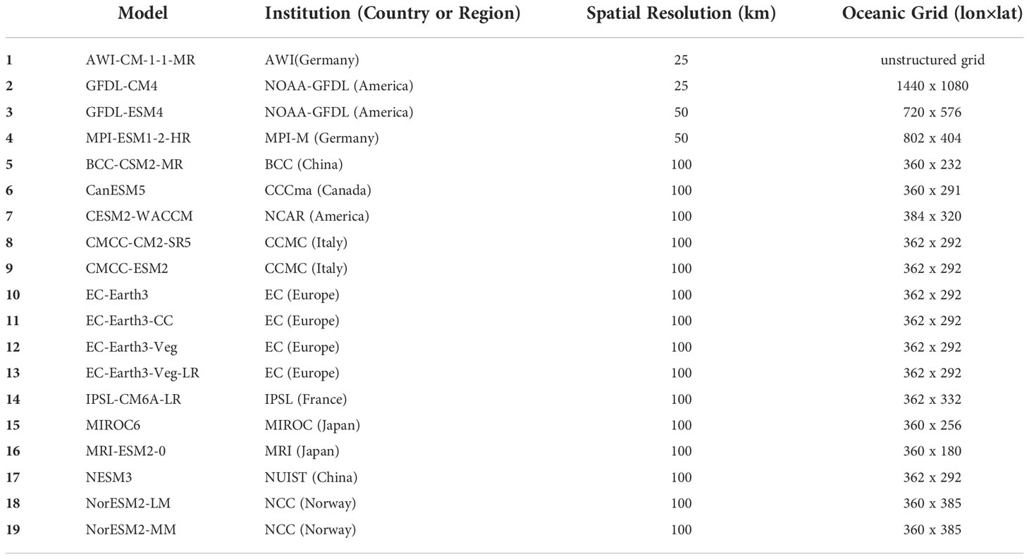
Table 1 Basic information of 19 models from CMIP6.

2.3 Definition of MHWs

This study follows the MHW identification method proposed by Hobday et al. (2016). An MHW event requires an SST above a certain threshold (green curve in Figure 1) for at least five consecutive days. This work adopts the 90th percentile of SST recorded in 33 years (1982 ~ 2014) as the threshold. It is calculated at each point of each day within an 11-day window centered on the calculation days of all years and then using a 31-day moving average on each Julian day. This method ensures that enough samples are used in the calculation. Thus, the obtained climate state and threshold can reflect the multi-year average and upper limit characteristics of the SST in the area and its seasonal change. If the maximum interval between consecutive events is less than or equal to two days, it is regarded as the same event (such as MHW 2 in Figure 1).

FIGURE 1

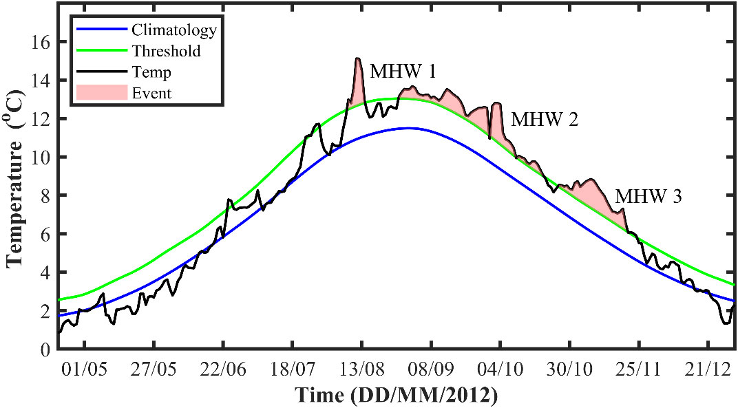
Figure 1 Identification of marine heatwaves at an arbitrary point (159.125°E, 49.125°N) in the WNPCC area between August 1 and December 21, 2012. The blue, green, and black curves represent the average climate temperature (1982 ~ 2014), the 90th percentile threshold value, and the point’s daily sea surface temperature curves, respectively. The reddish shading indicates three marine heatwave events.

Figure 1 shows three MHW cases identified at an arbitrary point (159.125°E, 49.125°N) in the WNPCC area. The reddish shading indicates three MHWs, occurring on August 08, 2012 ~ August 14, 2012 (MHW 1), August 27, 2012 ~ October 20, 2012 (MHW 2), and October 26, 2012 ~ November 20, 2012 (MHW 3). The average intensities of these three MHWs are 2.95, 1.98, and 2.01°C, respectively (Please refer to subsection 2.4 for specific definitions). For more detailed information about these three MHWs, please refer to Table S1 in the supporting information. The climate state and threshold from the OISSTV2 data (1982 ~ 2014) are also selected as the benchmark to detect MHWs in the projection period (2015 ~ 2100).

2.4 Characteristics of MHWs

The following six MHWs characteristics are selected for analysis. 1) Number: the total annual number of MHWs occurring at an arbitrary point in the WNPCC area. 2) Duration: the period from the beginning to the end of an MHW event. 3) Days: the total duration of all MHWs occurring at an arbitrary point within a year. 4) Cumulative-Intensity (CumInt): the cumulative sum of the difference between the daily SST and the corresponding climatic temperature during one MHW event. 5) Max-Intensity (MaxInt): the maximum difference between the daily SST and the corresponding climatic temperature during one MHW event. 6) Mean-Intensity (MeanInt): the average difference between the daily SST and the corresponding climatic temperature during one MHW event.

2.5 Optimal selection method for CMIP6 models

To evaluate the simulation ability of the 19 CMIP6 models, we compare the MHWs characteristics simulated by these models from 1982 to 2014 with the OISSTV2 data. The algorithm flowchart used in this study is shown in Figure 2. Seven evaluation indexes are selected to rank the simulation performance of the GCMs, assuming the proportion of each evaluation index is the same. Each index is assigned a value between 60 and 100 points, considering the difference between the GCMs and OISSTV2 data. The absolute deviation between the simulation parameters of each index (such as MHWs MeanInt) and the results from OISSTV2 is first calculated. The 19 models are then scored according to the calculated absolute deviation value using the following formula:

$\begin{array}{ll}{S}_i=\frac{f_{\max }-f_i}{f_{\max }-f_{\min }}\times 40+60,& (1)\end{array}$

FIGURE 2

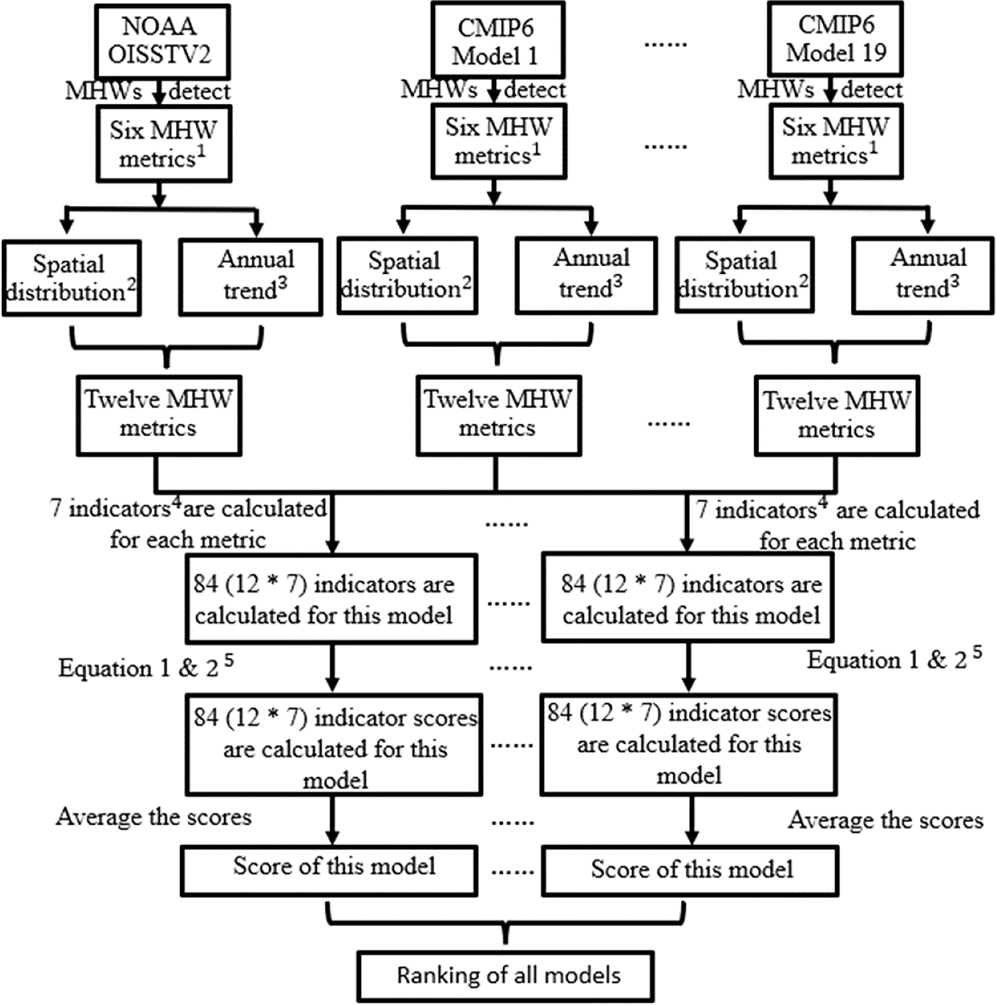
Figure 2 Flowchart summarizing the evaluation methods used in this study. ¹Six MHW metrics: Number, Duration, Days, CumInt, MaxInt and MeanInt. ²Spatial distribution: spatial distribution of multi-year average. ³Annual trend: spatially weighted average of annual average. ⁴Seven indicators: Root Mean Square Error, Mean Absolute Percentage Error, Correct-Recognition Rate, Under-Recognition Rate, Over-Recognition Rate, Regression Coefficient and Taylor Scores. ⁵Equation 1 & 2: Equation 1 for Taylor Scores and Correct-Recognition Rate, Equation 2 for the other five indicators. Equation 1: $Grade=\frac{x_i-x_{\min }}{x_{\max }-x_{\min }}\times 40+60$, Equation 2: $Grade=\frac{x_{\max }-x_i}{x_{\max }-x_{\min }}\times 40+60$.

where S_i is the index score for the characteristic parameter simulation. f_i represents the absolute deviation value between model i and OISSTV2. f_min and f_max are the minimum and maximum values of the absolute deviation, respectively, representing the deviation of the best and worst simulation results. After conversion, the simulation effect of each index on each MHWs characteristic is given a score between 60 and 100. Finally, the scores are ranked after equal weight averaging, and the top five models are selected for projection analysis of MHWs.

The seven correlation indicators are:

2.5.1 Root mean square error

$\begin{array}{ll}RMSE=\sqrt{\frac{{\sum }_{k=1}^N{(x_k-y_k)}^2}{N}}& (2)\end{array}$

where x_k and y_k represent the MHWs characteristics (e.g., MeanInt) from OISSTV2 and CMIP6 model, respectively, at an arbitrary point, and N represents the total grid points in the WNPCC area. RMSE represents the degree of dispersion between the results from the model and OISSTV2.

2.5.2 Mean absolute percentage error

$\begin{array}{ll}MAPE=\frac{1}{N }\sum _{k=1}^N\left|\frac{\left|x_k-y_k\right|}{x_k}\right|\times 100\%& (3)\end{array}$

The meaning of each symbol is the same as that in equation (2). MAPE represents the percentage of deviation between the model and OISSTV2.

2.5.3 Correct-recognition rate

$\begin{array}{ll}CRR=\frac{m_a}{N}\times 100\%& (4)\end{array}$

CRR represents the ratio of grid points (m_a ) in which both the CMIP6 models and OISSTV2 data detect MHWs to the total grid points (N ) in the WNPCC area.

2.5.4 Under-recognition rate

$\begin{array}{ll}URR=\frac{m_b}{N}\times 100\%& (5)\end{array}$

URR is the ratio of the grid points (m_b ) where the OISSTV2 data recognize MHWs but not the CMIP6 model data to the total grid points (N ) in the WNPCC area.

2.5.5 Over-recognition rate

$\begin{array}{ll}ORR=\frac{m_c}{N}\times 100\%& (6)\end{array}$

ORR indicates the ratio of the grid points (m_c ) where OISSTV2 data do not identify MHWs, but the CMIP6 model data incorrectly recognizes them as MHWs, to the total grid points (N ) in the WNPCC area.

2.5.6 Regression coefficient (k )

$\begin{array}{ll}{y}_k=k{x}_k+b,& (7)\end{array}$

where x_k and y_k represent MHWs characteristics identified by the CIMP6 and OISSTV2 data, respectively. The symbol b represents the intercept of the fitting line. Regression coefficient represents the slope of the regression curve obtained by performing linear regression on the MHWs parameters identified by the OISSTV2 and the CMIP6 data. The closer the coefficient to 1.0, the closer the simulated MHWs characteristic is to OISSTV2.

2.5.7 Taylor score

$\begin{array}{ll}TS=\frac{4{(1+R)}^4}{{\left(\frac{{\sigma }_m}{{\sigma }_0}+\frac{{\sigma }_0}{{\sigma }_m}\right)}^2{(1+R_0)}^4}& (8)\end{array}$

where R represents the correlation coefficient of MHW detection results between the CMIP6 and OISSTV2 data. R₀ is the maximum value of the correlation coefficient (taken as 1.0 in this study). σ_m and σ₀ represent the standard deviation of the MHWs characteristics’ spatial distribution from CMIP6 and OISSTV2, respectively. The Taylor score varies from 0.0 to 1.0 (Taylor, 2001). The larger the value, the closer the spatial distribution of the CMIP6 results is to OISSTV2.

Each MHW characteristic has two quantities: the spatial distribution of the average intensity in the WNPCC region and the annual trend of the regional average. Therefore, the above seven evaluation indicators correspond to fourteen evaluation scores (annual-RMSE, annual-MAPE, annual-CRR, annual-URR, annual-ORR, annual-k, annual-TS, mean-RMSE, mean-MAPE, mean-CRR, mean-URR, mean-ORR, mean-k, and mean-TS). However, since the mean-ORR scores in the 19 models are all 100 points (that is, there is no over-recognition phenomenon), only thirteen indicators are valid. Figure 3 presents the evaluation index scores and ranking of each model. The five top-performing CMIP6 models are GFDL-CM4, GFDL-ESM4, AWI-CM-1-1-MR, EC-Earth3-Veg and EC-Earth3. These models are used for the MHWs projection in Section 4.

FIGURE 3

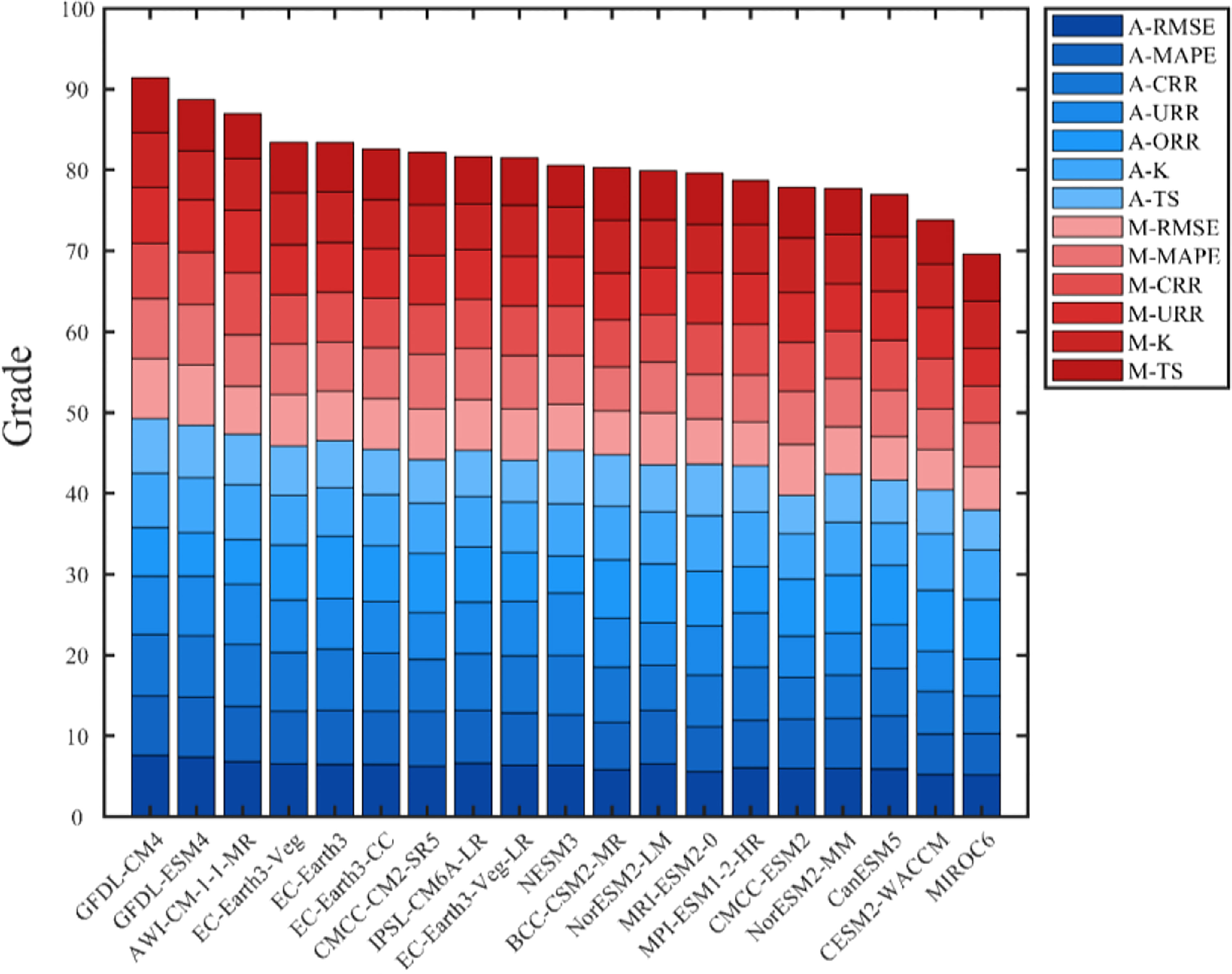
Figure 3 Evaluation scores for the 19 CMIP6 models. The thirteen color blocks from bottom to top correspond to thirteen weighted scoring indicators: annual-RMSE, annual-MAPE, annual-CRR, annual-URR, annual-ORR, annual-k, annual-TS, mean-RMSE, mean-MAPE, mean-CRR, mean-URR, mean-k, and mean-TS.

3 Historical characteristics of MHWs

3.1 Spatial distribution of MHWs characteristics

Figure 4 gives the spatial distribution of MHWs characteristics in the historical period (1982 ~ 2014) obtained from the OISSTV2 data. MHWs occur in most WNPCC areas, with an average number of 1.95 ± 0.21 times/year from 1982 to 2014 (Figure 4A). The number of MHWs is relatively low in the open ocean, especially in the southeast area of the WNPCC, while it is relatively high in the continental region. The region with the largest MHWs number is located at (122.125°E, 24.125°N), with 2.73 times/year.

FIGURE 4

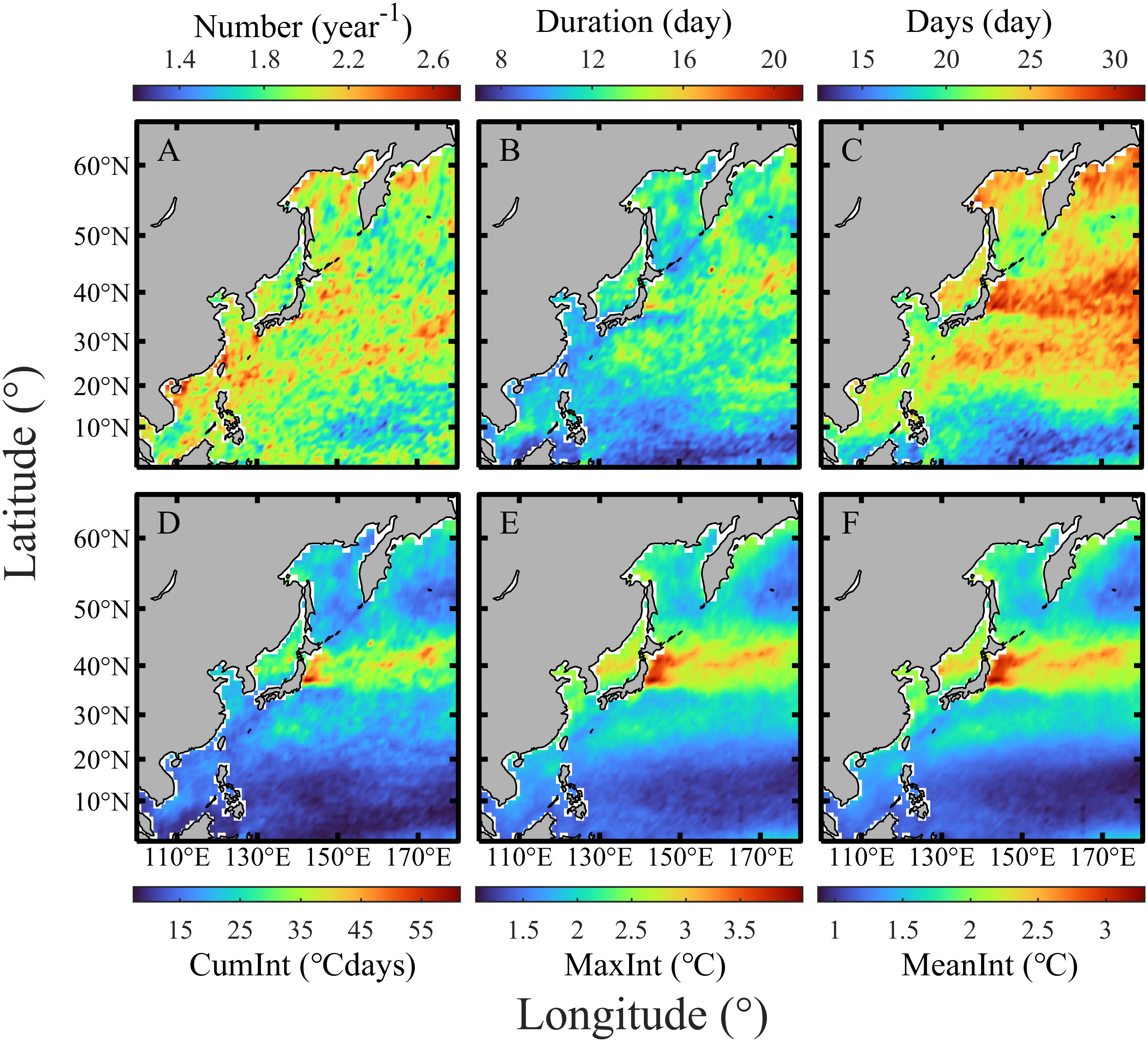
Figure 4 Spatial distribution of multi-year averages historical MHWs characteristics in the WNPCC area based on OISSTV2 data. Multi-year averages MHWs (A) Number (units: year^-1), (B) Duration (units: day), (C) Days (units: day), (D) CumInt (units: °C days), (E) MaxInt (units: °C), and (F) MeanInt (units: °C).

Figure 4B shows the multi-year average of MHWs duration from 1982 to 2014, with an average value of 11.38 ± 1.97 days. The maximum value is 21.26 days, which occurs at (158.125°E, 44.125°N). It should be noted that this maximum duration is the average annual result rather than the maximum value of each MHWs. The longest duration is 128 days (from November 8, 2010 to May 12, 2011), occurring at (172.125°E, 43.125°N). Unlike the distribution in Figure 4A, the multi-year average duration shows a more significant value in the open ocean than in the coastal area. That is, MHWs frequently occur in coastal areas but with relatively short duration.

Figure 4C gives the spatial distribution of the multi-year average MHWs days. It means the total durations of multiple MHWs in a year. The average value is 22.06 ± 3.84 days/year, and the maximum value is 31.79 days/year, which appears at (143.125°E, 37.125°N). Compared with Figure 4B, there is a more apparent meridional difference than in the MHWs duration. This difference is mainly because MHWs can occur several times in one year (Figure 4A). That is, Figure 4C is equivalent to the cumulative result of Figures 4A, B.

Figures 4D–F illustrate the multi-year average MHWs cumulative intensity, maximum intensity, and mean intensity in the historical period, with average values of 18.06 ± 7.67 °C days, 1.84 ± 0.50 °C and 1.49 ± 0.42 °C, respectively, and all appears at point (143.125°E, 37.125°N). The high intensity of MHWs in the WNPCC area is located in the Oyashio extension region. This distribution may be caused by the intersection of a cold current (Oyashio) and a warm current (Kuroshio) in this area. The intersection of cold and warm currents leads to significant changes in water temperature, which can induce strong MHWs. For more detailed information about the extreme value of MHWs characteristics, please refer to Table S2 in the supporting information. The discussion of specific physical mechanisms is beyond the scope of this study and will be addressed in future research.

3.2 Spatial distribution of the trend for MHWs characteristics

Figure 5A illustrates the trend of MHWs number from 1982 to 2014. The average value is 0.08 ± 0.04 times/year, and the maximum value is 0.20 times/year, located at (168.125°E, 57.125°N). It indicates an increase by about two more MHW events each decade. A negative value indicates the MHWs decreases, and the extreme value is -0.05 times/year, appearing at (148.125°E, 41.125°N). In the southeast WNPCC area, the trend of MHW number increases (Figure 5A) but with a low annual average frequency (Figure 4A).

FIGURE 5

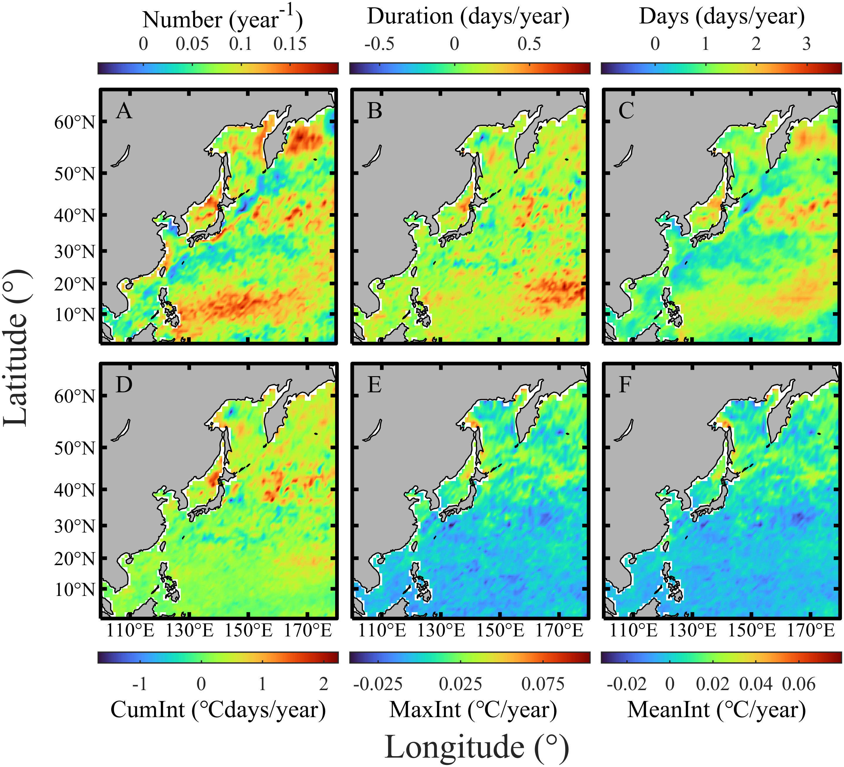
Figure 5 Spatial distribution of the MHWs characteristics trend during the historical period based on OISSTV2 data. Variation trend of MHWs (A) Number (units: year-1), (B) Duration (units: day), (C) Days (units: day), (D) CumInt (units: °C days), (E) MaxInt (units: °C), and (F) MeanInt (units: °C).

The trend of the MHW duration is given in Figure 5B. Its average value is 0.15 ± 0.16 days/year, and the maximum value is 0.90 days/year, appearing at (178.125°E, 18.125°N). This indicates that the average duration of each MHW gradually increases during the historical period. Figure 5C shows the trend of MHW days, with an average value of 1.17 ± 0.50 days/year. Its maximum value is 3.68 days/year, appearing at (164.125°E, 62.125°N).

Figures 5D–F show the annual trend of MHWs cumulative intensity, maximum intensity, and average intensity in the historical period. The average values are 0.26 ± 0.32 °Cdays/year, 0.003 ± 0.01 °C/year, and 0.001 ± 0.01 °C/year, respectively. The increasing trend of these three MHW characteristics is very homogenous in the WNPCC area. The maximum values are 2.24°Cdays/year, 0.10°C/year, and 0.08°C/year, which appear at (160.125°E, 40.125°N), (162.125°E, 58.125°N), and (162.125°E, 58.125°N), respectively. There are apparent high-value areas in Figures 4D–F, while the distribution in Figures 5D–F is relatively uniform. Please refer to Table S3 in the supporting information for more details about the extreme value for MHWs characteristics trends.

3.3 Annual average trend of MHWs characteristics

Figure 6 gives the annual trend of spatially-averaged historical MHWs characteristics in the WNPCC region. The MHWs number, duration, days, and CumInt have a significant increasing trend, with rates of 0.04 ± 0.01 times/year (Figure 6A), 0.11 ± 0.02 days/year (Figure 6B), 0.71 ± 0.18 days/year (Figure 6C), and 0.21 ± 0.06°C days/year (Figure 6D), respectively. However, the annual trend of the MaxInt (Figure 6E) and MeanInt (Figure 6F) are almost zero.

FIGURE 6

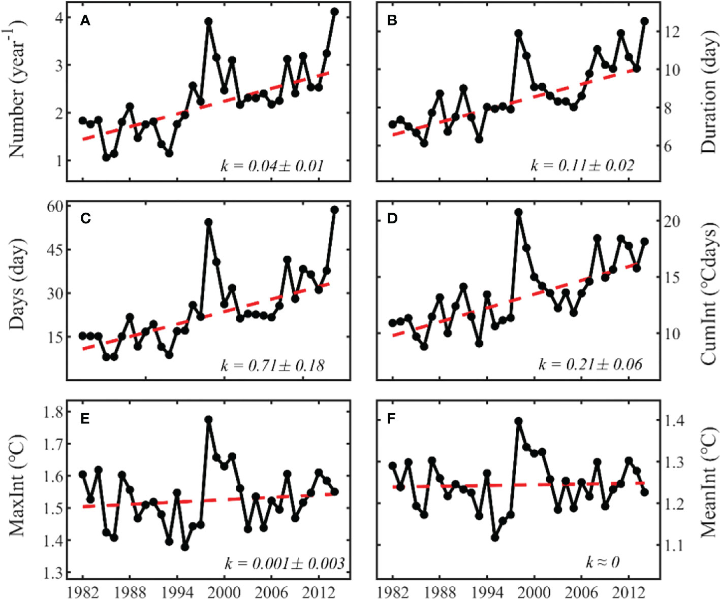
Figure 6 Annual trend of the spatially-averaged historical MHWs characteristics in the WNPCC area from OISSTV2 data. Annual trend of the MHWs (A) Number (units: year^-1), (B) Duration (units: day), (C) Days (units: day), (D) CumInt (units: °C days), (E) MaxInt (units: °C), and (F) MeanInt (units: °C).

4 Projection of MHWs characteristics

4.1 Spatial distribution of MHWs characteristics

Projection scenarios help us understand MHWs trends to formulate early corresponding countermeasures. In this study, the future scenarios SSP1-2.6, 2-4.5, and 5-8.5 of the five best-performing numerical models are analyzed. Only four models are used for evaluation under the SSP1-2.6 scenario since GFDL-CM4 does not simulate this scenario. Figures 7–9 show the spatial distribution of the multi-year average MHWs characteristics and their differences under the SSP2-4.5 and 5-8.5 scenarios (SSP5-8.5 minus SSP2-4.5). For the SSP1-2.6 scenario, please refer to the supporting information (Figures S1–S6). The MHWs number in the south of the WNPCC area is significantly higher than that in the north area (Figure 7A). The average value in the whole WNPCC region is 3.33 ± 0.87 times/year. For more detailed information about the extreme value of the MHWs characteristics under three different scenarios, please refer to Tables S4–S6 in the supporting information.

FIGURE 7

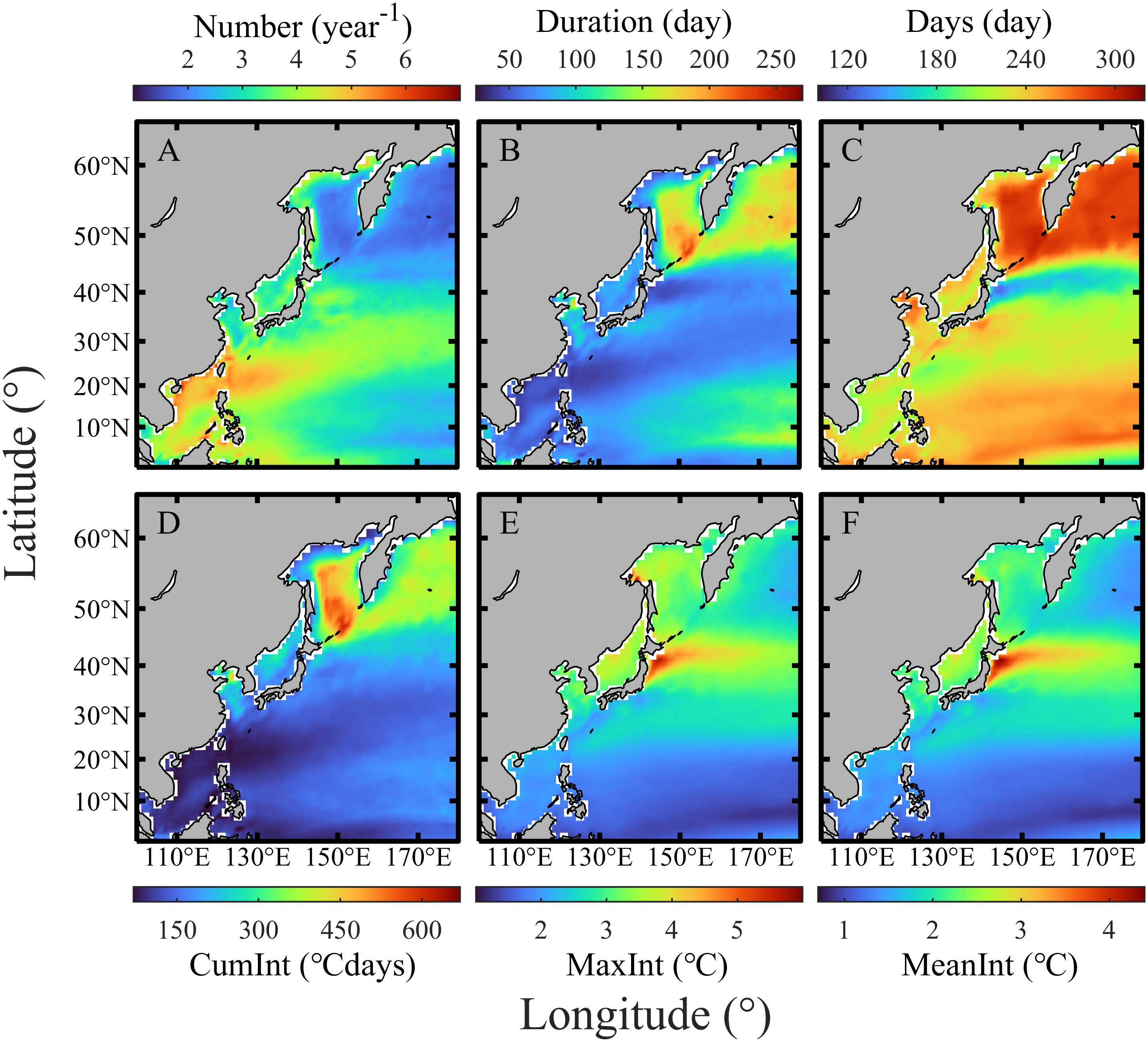
Figure 7 Spatial distribution of projected (2015 ~ 2100) MHWs characteristics in the WNPCC area under the SSP2-4.5 scenario. Multi-year average of MHWs (A) Number (units: year^-1), (B) Duration (units: day), (C) Days (units: day), (D) CumInt (units: °C days), (E) MaxInt (units: °C), and (F) MeanInt (units: °C).

Figure 8A is consistent with the overall distribution pattern of Figure 7A, with an average of 2.34 ± 0.59 times/year, which less than that in SSP2-4.5. The maximum value is 5.22 times/year, located at (118.125°E, 24.125°N), and the minimum is 1.17 times/year. Regardless of the average and maximum or minimum values, the multi-year average MHWs number in SSP5-8.5 (Figure 8A) is less than that in SSP1-2.6 (Figures S1, S4) and SSP2-4.5 (Figure 7A). Comparing the historical period (Figure 4A) with the three future scenarios, the MHWs number and the regional difference increase. The MHWs occurrence is significantly more frequent in the south than in the north of the WNPCC region.

FIGURE 8

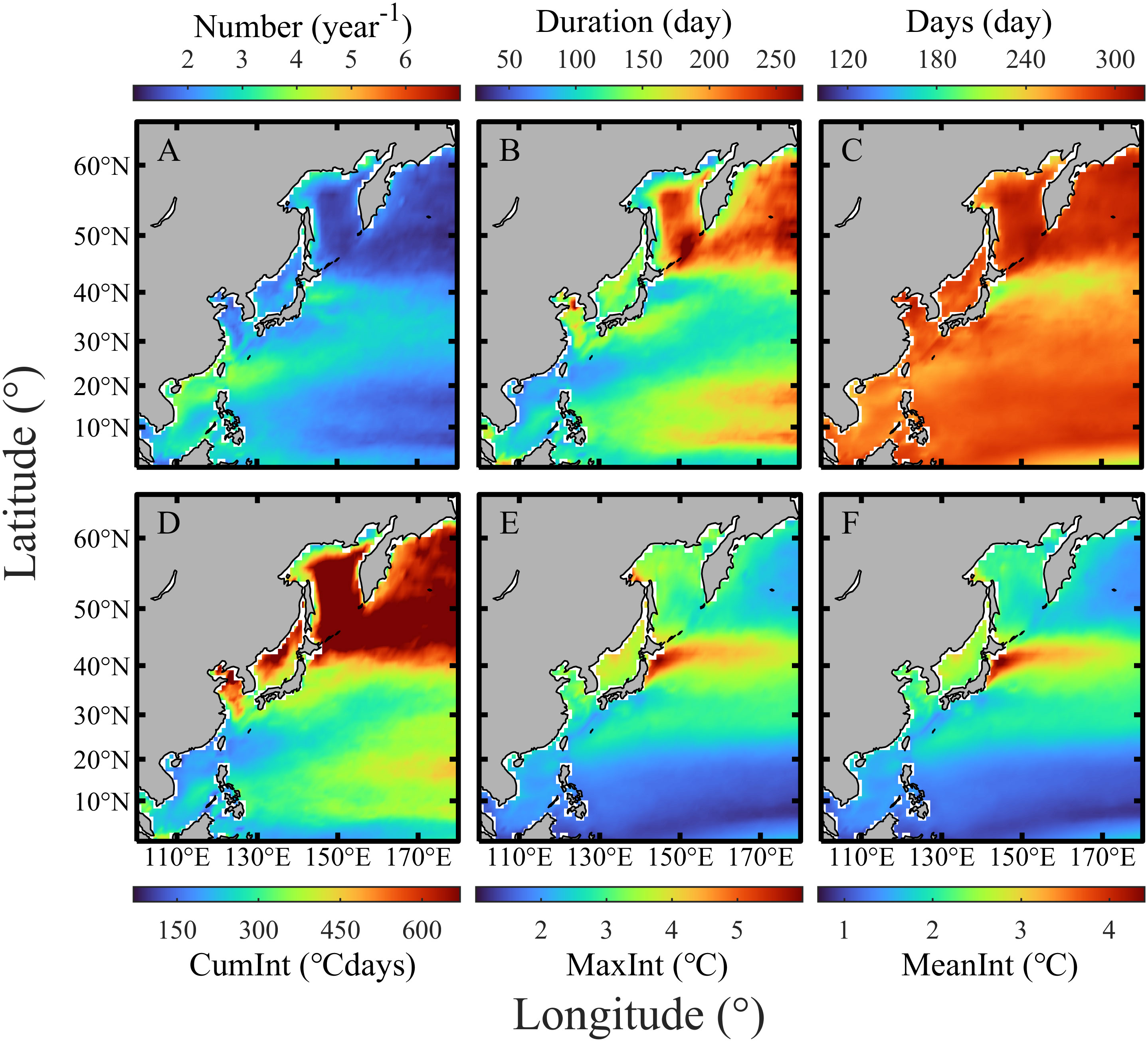
Figure 8 Spatial distribution of projected (2015 ~ 2100) MHWs characteristics in the WNPCC area under the SSP5-8.5 scenario. Multi-year average of (A) MHWs Number (units: year^-1), (B) Duration (units: day), (C) Days (units: day), (D) CumInt (units: °C days), (E) MaxInt (units: °C), and (F) MeanInt (units: °C).

Figures 7B, 8B show the spatial distribution of the multi-year average MHWs duration under SSP2-4.5 and SSP5-8.5 scenarios, respectively. The spatial distributions are almost the same in the two scenarios, showing larger values in the north of the WNPCC area than in the south. The spatial average of MHWs duration is 1.21 ± 0.49 days/year, 86.83 ± 35.58 days/year, and 138.66 ± 43.03 days/year under SSP1-2.6 (Figure S1), SSP2-4.5 (Figure 7B) and SSP5-8.5 scenario (Figure 8B), respectively. That is, the average MHWs duration increases significantly with an increase in emissions.

The average difference of MHWs duration in the WNPCC area shows a 51.82 ± 14.32 days longer duration under SSP5-8.5 than SSP2-4.5 (Figure 9B) and 83.77 ± 24.31 days longer duration than SSP1-2.6 (Figure S4). The maximum difference is 143.69 days/year, which occurs at (124.125°E, 37.125°N) between the SSP5-8.5 and SSP2-4.5. Compared with the historical MHW events in Figure 4B, the multi-year average MHWs duration in the future scenario significantly increases, and the difference in their spatial distribution is also more apparent. The MHWs duration is longer in the high-latitude area of the WNPCC region.

FIGURE 9

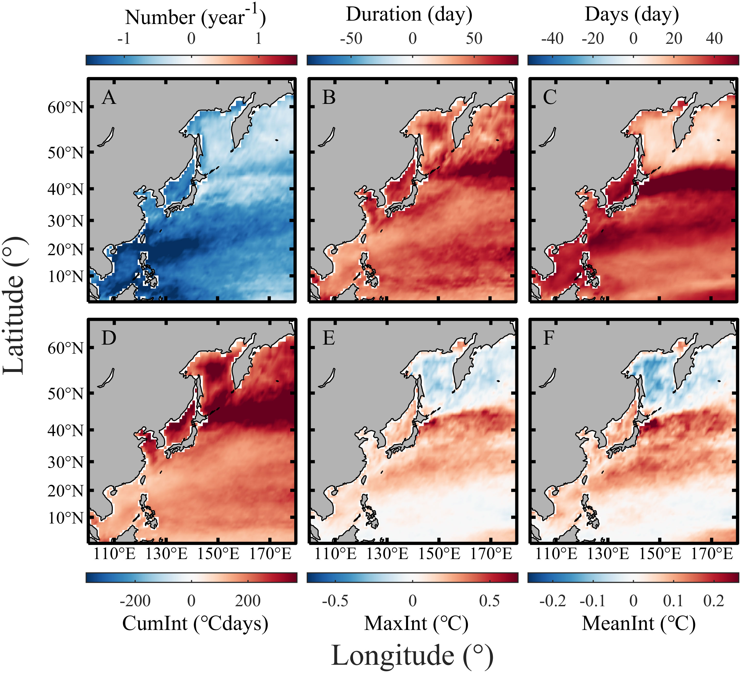
Figure 9 Spatial distribution of differences in projected MHWs characteristics under SSP2-4.5 and SSP5-8.5 scenarios (SSP5-8.5 minus SSP2-4.5). Multi-year average of (A) MHWs Number (units: year^-1), (B) Duration (units: day), (C) Days (units: day), (D) CumInt (units: °Cdays), (E) MaxInt (units: °C), and (F) MeanInt (units: °C).

The multi-year average MHWs days in Figures 7C, 8C show clear regional differences. The most noticeable feature is that the MHWs days in the Oyashio extension region are significantly shorter than in other areas. In the north of the Oyashio extension area (north of about 43°N) and south of 20°N, the MHWs days are relatively long. Under the SSP2-4.5, the longest MHWs cumulative days are 302.81 days, which occur at (156.125°E, 50.125°N), and the shortest days are 117.16 days, occurring at (142.125°E, 50.125°N). Accordingly, under SSP5-8.5, the longest MHWs days are 310.10 days, which occur at (170.125°E, 60.125°N), and the shortest days are 154.06 days, which occur at (137.125°E, 54.125°N). For more detailed information about the extreme value of the MHWs characteristics under the SSP1-2.6, 2-4.5, and 5-8.5 scenarios, please refer to Tables S4–S6 in the supporting information.

Under the SSP1-2.6, 2-4.5 and 5-8.5 scenarios, the average MHWs days in the WNPCC area are 184.93 ± 32.73, 236.50 ± 29.28, and 271.59 ± 18.50 days, respectively. Almost contrary to the spatial distribution of the annual MHWs days, the difference between the SSP5-8.5 and SSP2-4.5 scenarios is manifested in the Oyashio extension, the Subtropical Countercurrent, the Japan Sea, and the South China Sea areas (Figure 9C; Table S9). The differences between SSP2-4.5 and SSP1-2.6 (Figure S5), and SSP5-8.5 and SSP1-2.6 (Figure S6) have similar spatial distributions (please refer to see Tables S7 and S8 for more detailed information). This indicates that the response of MHWs days in different regions is different under different warming scenarios.

Figures 7D–F, 8D–F show the spatial distribution of MHWs CumInt, MaxInt, and MeanInt under SSP2-4.5 and 5-8.5 scenarios, respectively. In both scenarios, the high MHWs CumInt areas are distributed north of the Oyashio extension region. MaxInt and MeanInt are larger in the Oyashio extension than in other regions. Compared with the historical period (Figure 4D), the high-value CumInt region changes from the Oyashio extension region in the historical period to the high-latitude areas. MaxInt and MeanInt in the future scenario are consistent with the spatial distribution of the historical period. They are significantly enhanced in the mid-latitude area from 20°N to 43°N between SSP5-8.5 and 2-4.5 scenarios (Figures 9E, F). However, there is no noticeable change in other areas. Please refer to the supporting information for specific values between SSP2-4.5 and SSP1-2.6 (Table S7), SSP5-8.5 and SSP1-2.6 (Table S8), and SSP5-8.5 and SSP2-4.5 (Table S9).

4.2 Spatial distribution of MHWs characteristics variation ratio

Figures 10–12 illustrate the spatial distribution of the multi-year average trend for SSP2-4.5 and 5-8.5 scenarios and their differences (SSP5-8.5 minus SSP2-4.5). Figures 10A–11A show that, overall, the annual variation trend of the MHWs number is reduced by an average of -0.03 ± 0.01 and -0.06 ± 0.01 times/year, respectively. The reduction of MHWs number is the smallest in the mid-latitudes region (about 20°N ~ 43°N), especially in the Oyashio extension region. The fastest decrease ratio is at (131.125°E, 0.125°N), reaching -0.09 times/year for the SSP2-4.5 scenario, and at (119.125°E, 1.125°N), reaching -0.11 times/year for the SSP5-8.5 scenario. For the SSP1-2.6 scenario, please refer to Figure S2 in the supporting information.

FIGURE 10

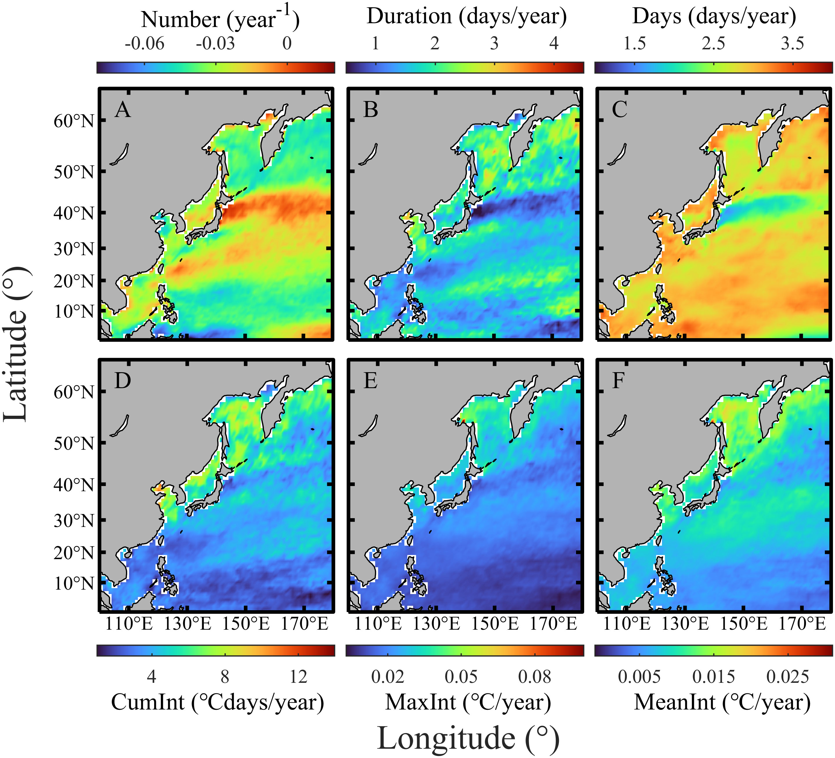
Figure 10 Spatial distribution of average annual variation ratio for MHWs characteristics under the SSP2-4.5 scenario. Average of annual variation ratio for MHWs (A) Number (units: year^-1), (B) Duration (units: day/year), (C) Days (units: day/year), (D) CumInt (units: °Cdays/year), (E) MaxInt (units: °C/year), and (F) MeanInt (units: °C/year).

FIGURE 11

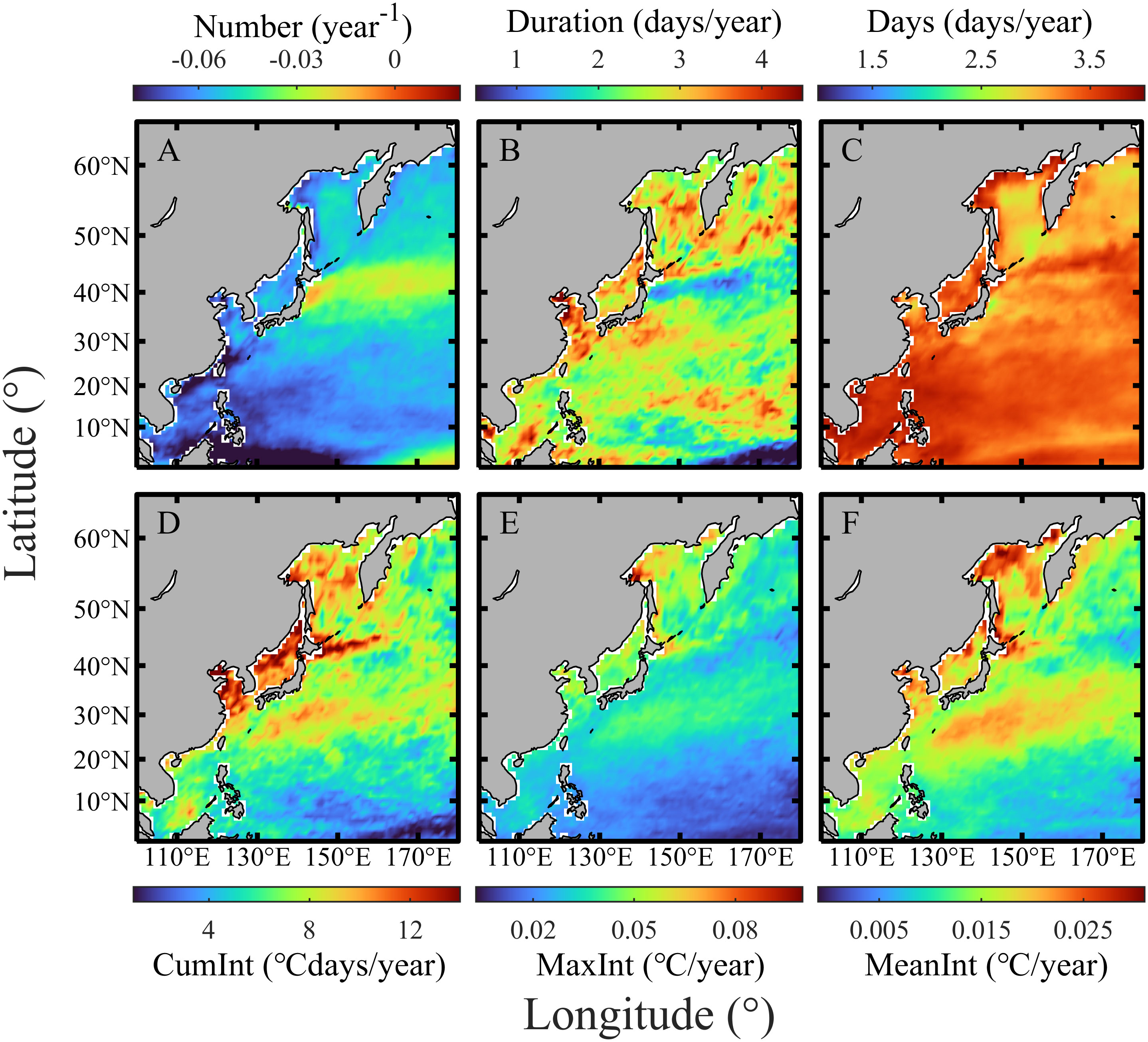
Figure 11 Spatial distribution of average annual variation ratio for MHWs characteristics under the SSP5-8.5 scenario. Average of annual variation ratio for MHWs (A) Number (units: year^-1), (B) Duration (units: day/year), (C) Days (units: day/year), (D) CumInt (units: °Cdays/year), (E) MaxInt (units: °C/year), and (F) MeanInt (units: °C/year).

Figure 12A shows that the multi-year average trend for MHWs number is lower in SSP5-8.5 than in SSP2-4.5, and its average value is -0.03 ± 0.01 times/year. These two scenarios have significant spatial differences. The annual variation ratio for the MHWs frequency in the South China Sea, the East China Sea, and the east side of Taiwan island is more significant than in other regions. This result indicates the regional difference in MHWs characteristics response under different warming scenarios. For more detailed information about the extreme value of the MHWs characteristics trend under SSP1-2.6, 2-4.5 and 5-8.5 scenarios, please refer to Tables S10–S12, respectively, in the supporting information.

FIGURE 12

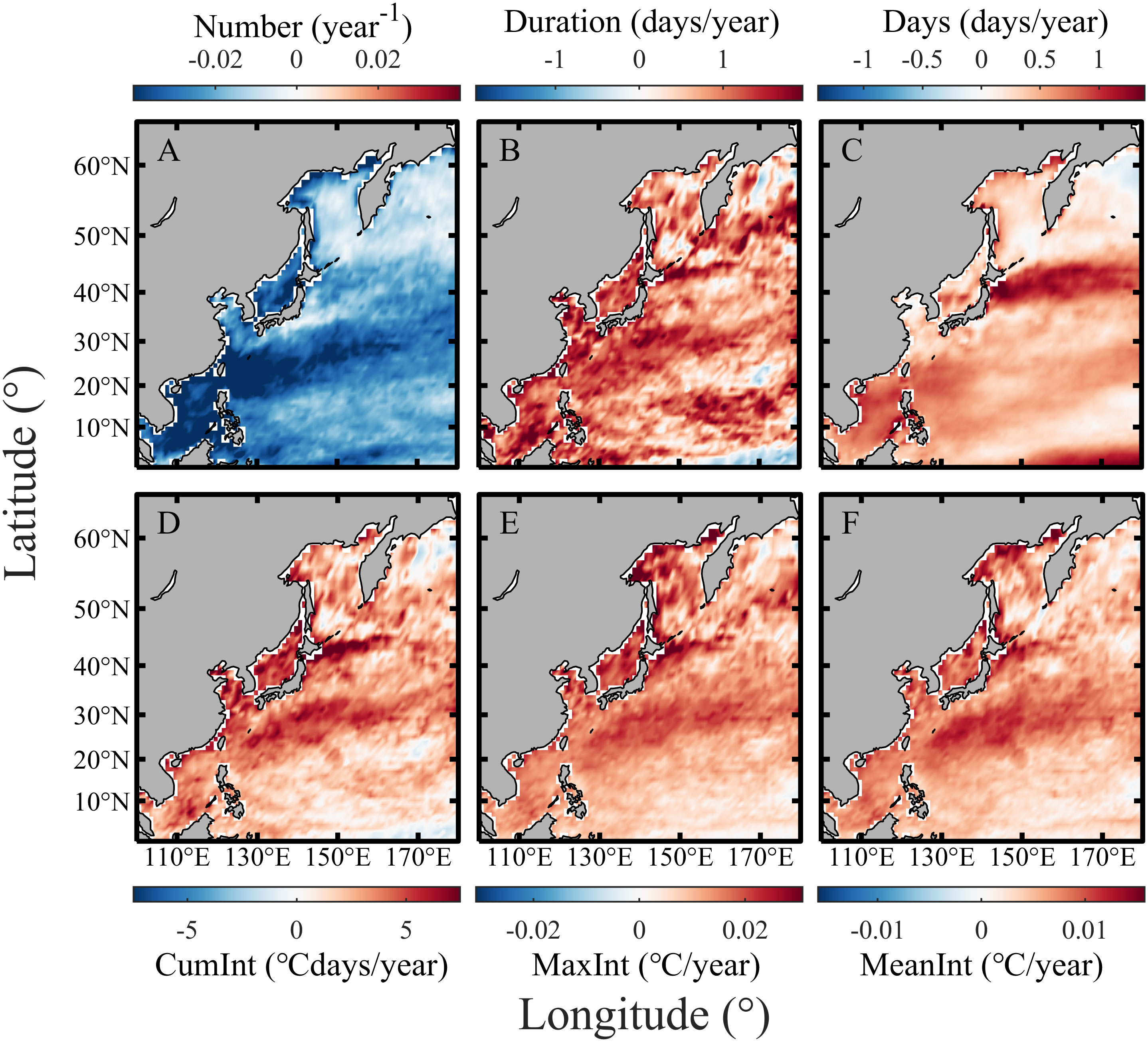
Figure 12 Spatial distribution of differences in projected annual variation ratio of MHWs characteristics for the SSP2-4.5 and 5-8.5 (SSP5-8.5 minus SSP2-4.5). Average annual variation ratio differences for MHWs (A) Number (units: year^-1), (B) Duration (units: day/year), (C) Days (units: day/year), (D) CumInt (units: °Cdays/year), (E) MaxInt (units: °C/year), and (F) MeanInt (units: °C/year).

The average value of MHWs duration is 0.51 ± 0.34, 1.62 ± 0.44 and 2.56 ± 0.70 days/year for the SSP1-2.6 (Figure S2B), 2-4.5 (Figure 10B), and 5-8.5 scenario (Figure 11B), respectively. The maximum annual average duration variation ratio reaches 4.78 days/year at (119.125°E, 37.125°N) for SSP2-4.5. Correspondingly, for the SSP5-8.5 scenario, the maximum annual average duration variation ratio reaches 5.64 days/year, which occurs at (100.125°E, 5.125°N). From Figure 12B, the annual average duration variation ratio is more significant under SSP5-8.5 than under SSP2-4.5, and the regional average value is 0.94 ± 0.61 days/year. Please refer to Tables S13–S15 in the supporting information for the extreme value distribution of the spatial difference among these three scenarios.

Under the SSP2-4.5 scenario, the average variation ratio of MHWs days is 2.85 ± 0.28 days/year (Figure 10C). Accordingly, in the SSP5-8.5 scenario, it is 3.38 ± 0.24 days/year (Figure 11C). The variation ratio of MHWs days is larger under SSP5-8.5 than under the SSP2-4.5 scenario, with an average value of 0.53 ± 0.32 days/year (Figure 12C). The variation ratios under these two scenarios also have spatial differences, especially in the Oyashio extension and the South China Sea regions. For the differences among the SSP1-2.6, 2-4.5 and 5-8.5 scenarios, please refer to Figures S5, S6 in the supporting information.

Figures 10D–F, 11D–F show the spatial distribution of the annual variation ratio of MHWs cumulative intensity, maximum intensity, and mean intensity under the SSP2-4.5 and SSP5-8.5 scenarios, respectively. Under the SSP2-4.5 scenario, the spatial distribution of these three characteristics is relatively uniform, and their spatial average values in the WNPCC area are 3.83 ± 1.43°C days/year, 0.02 ± 0.01°C/year, and 0.01 ± 0.003°C/year, respectively. Correspondingly, under the SSP5-8.5 scenario, its spatial average value is 6.70 ± 2.61 °Cdays/year, 0.03 ± 0.01°C/year, and 0.01 ± 0.01 °C/year. Figures 12D–F show that the annual variation ratio for the MHWs cumulative intensity, maximum intensity, and mean intensity is more significant in the SSP5-8.5 than in the SSP2-4.5 scenario. In terms of spatial distribution, the Oyashio extension and the Subtropical Countercurrent regions are more intense than other areas. Please refer to Table S10 in the supporting information for the extreme value distribution of the variation ratio for MHWs cumulative intensity, maximum intensity, and mean intensity under the SSP1-2.6.

4.3 Future trend of the MHWs in the WNPCC region

Figure 13 illustrates the future trend of MHWs characteristics under the SSP1-2.6, 2-4.5 and 5-8.5 scenarios. The MHWs number has a two-segment distribution (Figure 13A). It has an increasing trend from 2015 to 2036, with a growth rate of 0.01 ± 0.01, 0.03 ± 0.01, and 0.03 ± 0.01 times/year for SSP1-2.6, 2-4.5 and 5-8.5 scenarios, respectively. From 2036 to 2100, it shows a decreasing trend, with an average decreasing rate of -0.002 ± 0.002, -0.03 ± 0.002, and -0.04 ± 0.003 times/year for SSP1-2.6, 2-4.5, and 5-8.5 scenarios, respectively. In short, the MHWs number gradually increases before 2036, and it decreases yearly due to the growth in the MHWs duration (Figure 13B).

FIGURE 13

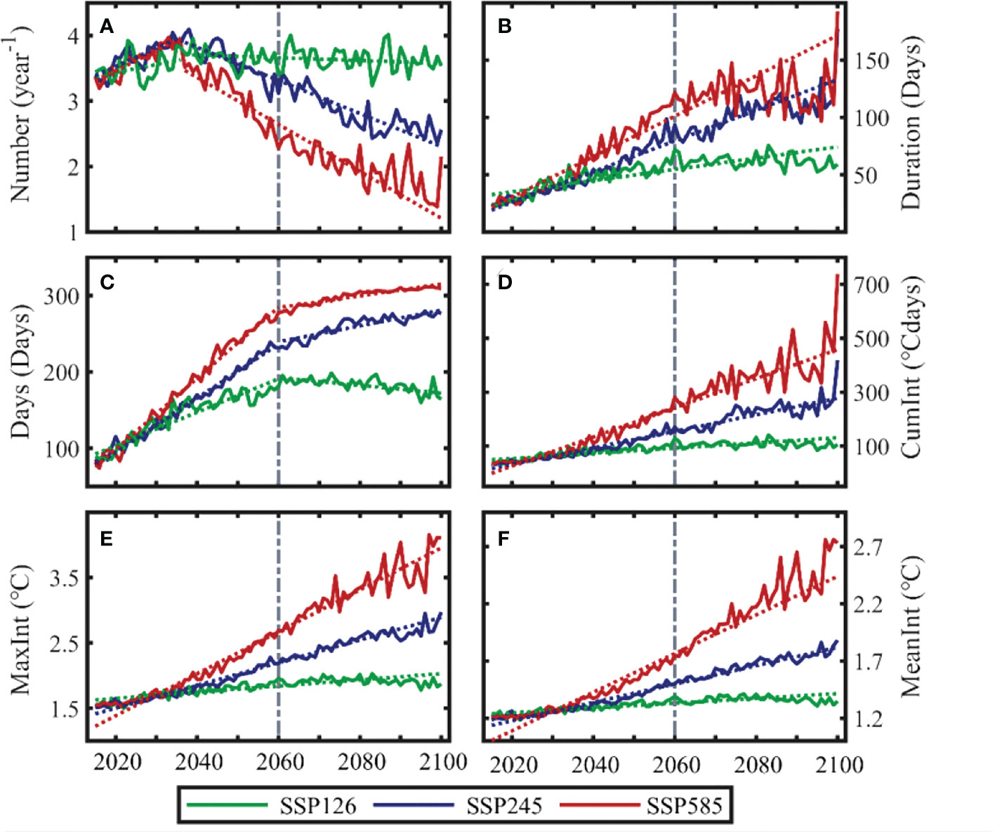
Figure 13 Projected interannual variability of MWHs parameters under the SSP1-2.6 (green line), SSP2-4.5 (blue line) and SSP5-8.5 (red line) scenarios from the ensemble mean of the four/five/five selected models. The solid line is the future change of the estimated parameters, and the dotted line is the linear regression result. The left side of the dotted line (2060) represents the near future scenario, and the right side of the dotted line represents the far future scenario. Interannual variability for MHWs (A) Number (unit: year^-1), (B) Duration (unit: day), (C) Days (unit: day), (D) CumInt (units: °C days), (E) MaxInt (units: °C), (F) MeanInt (units: °C).

Under the SSP1-2.6, 2-4.5 and 5-8.5 scenarios, the average MHWs duration increases by 0.49 ± 0.06, 1.34 ± 0.05, and 1.76 ± 0.10 days/year (Figure 13B). Before 2060, the duration for a single MHW increases rapidly (Figure 13C). The growth rates for the SSP1-2.6, 2-4.5 and 5-8.5 scenarios are 2.19 ± 0.21, 3.53 ± 0.12 and 4.64 ± 0.16 days/year, respectively. After 2060, the rate of increase slows down to -0.51 ± 0.15 (SSP1-2.6), 1.03 ± 0.14 (SSP2-4.5) and 0.77 ± 0.10 days/year (SSP5-8.5), respectively.

From the MHWs cumulative intensity (Figure 13D), maximum intensity (Figure 13E), and average intensity (Figure 13F), the projected MHW has a significant increasing trend, and the increase is more evident under the SSP5-8.5 than the other two scenarios. The growth rates are 0.96 ± 0.11 °C days/year, 0.005 ± 0.001°C/year and 0.002 ± 0.0002°C/year for the SSP1-2.6 scenario; 3.07 ± 0.12 °C days/year, 0.02 ± 0.001 °C/year, and 0.01 ± 0.0003 °C/year for the SSP2-4.5 scenario; and 5.41 ± 0.21 °C days/year, 0.03 ± 0.001 °C/year, and 0.02 ± 0.001 °C/year for the SSP5-8.5 scenario, respectively. For more detailed value information, please refer to Table S16 in the supporting information. Some previous studies divided the future simulation period into the near future (before 2060) and far future (from 2060 to 2100). However, it can be seen from Figure 13 that apart from the MHWs days, which have obvious differences around 2060, the other five variables have no particularly obvious differences. Therefore, this study does not separate the future period into near and far futures for discussion. This phenomenon may be because we use the fixed threshold method to detect MHWs.

5 Discussion

5.1 Seasonal variation of MHWs characteristics

The seasonal difference in MHWs is a fascinating scientific problem. We calculated the monthly change of the MHWs occurrence area percentage (Figure 14A) and the MHWs average intensity (Figure 14B) in the WNPCC area. The MHWs occurrence area percentage is defined as $\frac{S_1}{S_2}\times 100\%$, where S₁ represents the size occupied by the MHWs, and S₂ represents the total size of the WNPCC area. From Figure 14A, the occurrence area proportion in the future scenario is significantly larger than that in the historical period. The MHWs occurrence area in summer is slightly smaller than in winter.

FIGURE 14

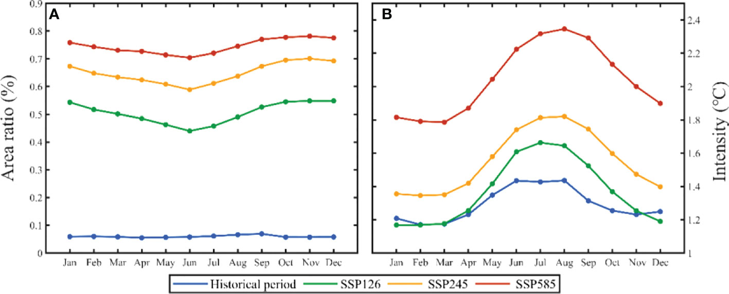
Figure 14 Monthly distribution of MHWs occurrence area percentage (A) and MHWs mean intensity (B) in the WNPCC area. The blue, green, yellow, and red curves represent the historical period, and the projection period under the SSP1-2.6, 2-4.5 and 5-8.5 scenarios, respectively.

In terms of MHWs intensity, both historical and future scenarios show prominent characteristics of strong in summer and weak in winter (Figure 14B). Under the SSP1-2.6 (2-4.5, 5-8.5) scenario, the maximum intensity of the MHW reaches 1.66°C (1.82°C, 2.35°C) in August, and the minimum intensity in March (February, March), reaches 1.17°C (1.35°C, 1.79°C). Accordingly, in the historical period, the maximum MHW intensity occurs in August, reaching 1.44°C, and the minimum value occurs in February, reaching 1.17°C.

5.2 Impact of different climate thresholds

The MHW’s definition is closely related to the selection of climate state threshold. Since the world’s oceans have a long-term warming trend, using a fixed climate threshold causes a significant increase in MHWs (Chiswell, 2022). On the other hand, some marine species have quickly adapted to the temperature rise, so the MHW defined by the fixed threshold may not be harmful to them. With the rise in the climate temperature baseline under global warming, ecosystems may be reorganized (Smale et al., 2019). That is, the MHW deformation method with a fixed threshold is suitable for marine species with weak temperature adaptability. However, it is not applicable for species with strong temperature adaptability. This leads to results such as no obvious marine disasters, although an MHW has occurred, thus breaking away from the significance of MHW studies. This problem can be overcome to a certain extent by moving the average temperature of the climate state, for example, using the 20 or 30-year moving average threshold of the climate state.

Establishing a good relationship between the definition and intensity of MHW and its possible impact can provide a practical and effective reference for the prediction of MHW and policy formulation of ocean management departments. In addition, the definition of MHW should consider the impact of global warming and the characteristics of local marine ecological communities. There are also views that MHW can be measured by “thermal displacement”, or the distance required to move to the same level of climate temperature habitat. However, this MHW definition applies to swimming marine species but is less applicable to immovable or benthic entities (including corals).

5.3 Subsurface MHWs

Current MHW discussions are usually based on SST data, i.e., MHW is a phenomenon occurring in the upper ocean layer. However, the warming phenomenon in the upper layer can contribute heat to the oceanic subsurface or even the interior through some physical processes (such as mesoscale eddy, Wang et al., 2022d). The surface warming caused by MHW in the northeast Pacific may penetrate the oceanic subsurface when the mixing is intense in winter (Scannell et al., 2020). In southeast Australia, Schaeffer and Roughan (2017) also found the enhancement of MHWs in the oceanic subsurface.

In addition to the influence of these surface MHWs on the oceanic subsurface layer, some studies have found that MHWs can occur directly in subsurface layers without the induction of surface warming. Hu et al. (2021) explored the subsurface MHW of the tropical western Pacific Ocean using high-resolution data collected by the Tropical Atmosphere Ocean/Triangle Trans-Ocean Buoy Network (TAO/TRITON) buoy. They pointed out that this particularly strong subsurface MHW seems unrelated to the warming of the ocean’s surface.

6 Conclusions

The MHWs spatial distribution characteristics and variation trends in the WNPCC area are analyzed during the historical period (1982 ~ 2014) using OISSTV2 data. With the results from OISSTV2 data as a comparison standard, five best-performing models are selected from 19 CMIP6 GCMs. Using the simulation results of these five models, the MHWs characteristics from 2015 to 2100 are studied under the SSP1-2.6, 2-4.5, and 5-8.5 scenarios. We also discuss the seasonal differences in the MHWs occurrence area and its intensity. The main conclusions are summarized as follows.

1. In the historical period, MHWs occur in most WNPCC areas, with an average number, duration, days, cumulative intensity, maximum intensity, and mean intensity of 1.95 ± 0.21 times/year, 11.38 ± 1.97 days, 22.06 ± 3.84 days, 18.06 ± 7.67 °Cdays, 1.84 ± 0.50°C, and 1.49 ± 0.42°C. The MHWs frequency is relatively low in the open ocean, especially in the southeast of the WNPCC area, while it is relatively high in the coastal region.

2. According to the optimization method proposed in this study, among the 19 CMIP6 GCMs, the five models that best reproduce MHWs in the WNPCC area relative to OISSTV2 are GFDL-CM4, GFDL-ESM4, AWI-CM-1-1-MR, EC-Earth3-Veg, and EC-Earth3.

3. In the future scenario (2015 ~ 2100), the projected MHWs characteristics under the SSP5-8.5 are more substantial than those under the SSP1-2.6 and SSP2-4.5, except for the MHWs frequency. The MHWs cumulative intensity is 96.36 ± 56.30, 175.44 ± 92.62, and 385.22 ± 168.00 °C days under the SSP1-2.6, 2-4.5 and 5-8.5, respectively. The maximum and average intensity of the MHWs in the Oyashio extension region are more robust than in other areas.

4. The annual variation ratio for the MHWs frequency is significant in the South China Sea, the East China Sea, and east side of Taiwan island. The annual average variation ratio of MHWs duration and cumulative days is more significant under the SSP5-8.5 than under SSP1-2.6 and 2-4.5.

5. The MHWs occurrence area in summer is slightly smaller than in winter, but the MHWs average intensity is stronger in summer than in winter.

Data availability statement

The original contributions presented in the study are included in the article/Supplementary Material. Further inquiries can be directed to the corresponding author.

Author contributions

YY, WS, JY, and CD conceived and designed the experiments. YY performed the experiments. WS, YY, JY, and JJ analyzed the data. WS and YY drafted the original manuscript. WS, YY, KL, JJ, and JY revised and edited the manuscript. All authors contributed to the article and approved the submitted version.

Funding

This study was supported by the National Natural Science Foundation of China under contract Nos. 42192562, 41906008, 51909100; the Open Fund of State Key Laboratory of Satellite Ocean Environment Dynamics, Second Institute of Oceanography, MNR under contract No. QNHX2231; the Innovation Group Project of Southern Marine Science and Engineering Guangdong Laboratory (Zhuhai) under contract No. 311020004; the National Natural Science Foundation of China under contract No. 42076162; and the Natural Science Foundation of Guangdong Province of China under contract No. 2020A1515010496.

Acknowledgments

We acknowledge the World Climate Research Programme’s (WCRP) Working Group on Coupled Modelling, which is responsible for coordinating CMIP. We also thank the climate modeling groups for producing and making available their model output. We thank Zijie Zhao for providing the main function code to detect marine heatwaves (https://github.com/ZijieZhaoMMHW/m_mhw1.0).

Conflict of interest

The authors declare that the research was conducted in the absence of any commercial or financial relationships that could be construed as a potential conflict of interest.

Publisher’s note

All claims expressed in this article are solely those of the authors and do not necessarily represent those of their affiliated organizations, or those of the publisher, the editors and the reviewers. Any product that may be evaluated in this article, or claim that may be made by its manufacturer, is not guaranteed or endorsed by the publisher.

Supplementary material

The Supplementary Material for this article can be found online at: https://www.frontiersin.org/articles/10.3389/fmars.2022.1048557/full#supplementary-material

References

Arias-Ortiz A., Serrano O., Masqué P., Lavery P. S., Mueller U., Kendrick G. A., et al. (2018). A marine heatwave drives massive losses from the world’s largest seagrass carbon stocks. Nat. Clim. Change. 8 (4), 338–344. doi: 10.1038/s41558-018-0096-y

CrossRef Full Text | Google Scholar

Benthuysen J. A., Oliver E. C. J., Feng M., Marshall A. G. (2018). Extreme marine warming across tropical Australia during austral summer 2015–2016. J. Geophys. Res. 123 (2), 1301–1326. doi: 10.1002/2017JC013326

CrossRef Full Text | Google Scholar

Black E., Blackburn M., Harrison G., Hoskins B., Methven J. (2004). Factors contributing to the summer 2003 European heatwave. Weather. 59 (8), 217–223. doi: 10.1256/wea.74.04

CrossRef Full Text | Google Scholar

Bond N. A., Cronin M. F., Freeland H., Mantua N. (2015). Causes and impacts of the 2014 warm anomaly in the NE pacific. Geophys. Res. Lett. 42 (9), 3414–3420. doi: 10.1002/2015GL063306

CrossRef Full Text | Google Scholar

Capotondi A., Newman M., Xu T., Di Lorenzo E. (2022). An optimal precursor of northeast pacific marine heatwaves and central pacific El niño events. Geophys. Res. Lett. 49 (5), e2021G–e97350. doi: 10.1029/2021GL097350

CrossRef Full Text | Google Scholar

Caputi N., Kangas M., Chandrapavan A., Hart A., Feng M., Marin M., et al. (2019). Factors affecting the recovery of invertebrate stocks from the 2011 western australian extreme marine heatwave. Front. Mar. Sci. 6. doi: 10.3389/fmars.2019.00484

CrossRef Full Text | Google Scholar

Caputi N., Kangas M., Denham A., Feng M., Pearce A., Hetzel Y., et al. (2016). Management adaptation of invertebrate fisheries to an extreme marine heat wave event at a global warming hot spot. Ecol. Evol. 6 (11), 3583–3593. doi: 10.1002/ece3.2137

PubMed Abstract | CrossRef Full Text | Google Scholar

Cavole L., Demko A., Diner R., Giddings A., Koester I., Pagniello C., et al. (2016). Biological impacts of the 2013–2015 warm-water anomaly in the northeast pacific: Winners, losers, and the future. Oceanography 29 (2), 273–285. doi: 10.5670/oceanog.2016.32

CrossRef Full Text | Google Scholar

Chandrapavan A., Caputi N., Kangas M. I. (2019). The decline and recovery of a crab population from an extreme marine heatwave and a changing climate. Front. Mar. Sci. 6. doi: 10.3389/fmars.2019.00510

CrossRef Full Text | Google Scholar

Chiswell S. M. (2022). Global trends in marine heatwaves and cold spells: The impacts of fixed versus changing baselines. J. Geophys. Res. 127, e2022JC018757. doi: 10.1029/2022JC018757

CrossRef Full Text | Google Scholar

Di Lorenzo E., Mantua N. (2016). Multi-year persistence of the 2014/15 north pacific marine heatwave. Nat. Clim. Change. 6 (11), 1042–1047. doi: 10.1038/nclimate3082

CrossRef Full Text | Google Scholar

Eyring V., Bony S., Meehl G. A., Senior C. A., Stevens B., Stouffer R. J., et al. (2016). Overview of the coupled model intercomparison project phase 6 (CMIP6) experimental design and organization. Geosci. Model. Dev. 9 (5), 1937–1958. doi: 10.5194/gmd-9-1937-2016

CrossRef Full Text | Google Scholar

Feng Y., Bethel B. J., Dong C., Zhao H., Yao Y., Yu Y. (2022). Marine heatwave events near weizhou island, beibu gulf in 2020 and their possible relations to coral bleaching. Sci. Total Environ. 823, 153414. doi: 10.1016/j.scitotenv.2022.153414

PubMed Abstract | CrossRef Full Text | Google Scholar

Frölicher T. L., Fischer E. M., Gruber N. (2018). Marine heatwaves under global warming. Nature. 560 (7718), 360–364. doi: 10.1038/s41586-018-0383-9

PubMed Abstract | CrossRef Full Text | Google Scholar

Gao G., Marin M., Feng M., Yin B., Yang D., Feng X., et al. (2020). Drivers of marine heatwaves in the East China Sea and the south yellow sea in three consecutive summers during 2016–2018. J. Geophys. Res. 125 (8), e2020J–e16518. doi: 10.1029/2020JC016518

CrossRef Full Text | Google Scholar

Garrabou J., Coma R., Bensoussan N., Bally M., Chevaldonne P., Cigliano M., et al. (2009). Mass mortality in northwestern Mediterranean rocky benthic communities: Effects of the 2003 heat wave. Global Change Biol. 15 (5), 1090–1103. doi: 10.1111/j.1365-2486.2008.01823.x

CrossRef Full Text | Google Scholar

Garrabou J., Gómez Gras D., Medrano A., Cerrano C., Ponti M., Schlegel R., et al. (2022). Marine heatwaves drive recurrent mass mortalities in the Mediterranean Sea. Global Change Biol. 28 (19), 5708–5725. doi: 10.1111/gcb.16301

CrossRef Full Text | Google Scholar

Hamed M. M., Nashwan M. S., Shiru M. S., Shahid S. (2022). Comparison between CMIP5 and CMIP6 models over MENA region using historical simulations and future projections. Sustainability. 14 (16), 10375. doi: 10.3390/su141610375

CrossRef Full Text | Google Scholar

Han W., Zhang L., Meehl G. A., Kido S., Tozuka T., Li Y., et al. (2022). Sea Level extremes and compounding marine heatwaves in coastal Indonesia. Nat. Commun. 13 (1), 6410. doi: 10.1038/s41467-022-34003-3

PubMed Abstract | CrossRef Full Text | Google Scholar

Hobday A. J., Alexander L. V., Perkins S. E., Smale D. A., Straub S. C., Oliver E. C. J., et al. (2016). A hierarchical approach to defining marine heatwaves. Prog. Oceanogr. 141, 227–238. doi: 10.1016/j.pocean.2015.12.014

CrossRef Full Text | Google Scholar

Holbrook N. J., Hernaman V., Koshiba S., Lako J., Kajtar J. B., Amosa P., et al. (2022). Impacts of marine heatwaves on tropical western and central pacific island nations and their communities. Global Planet. Change. 208, 103680. doi: 10.1016/j.gloplacha.2021.103680

CrossRef Full Text | Google Scholar

Holbrook N. J., Scannell H. A., Sen Gupta A., Benthuysen J. A., Feng M., Oliver E. C. J., et al. (2019). A global assessment of marine heatwaves and their drivers. Nat. Commun. 10 (1), 2624. doi: 10.1038/s41467-019-10206-z

PubMed Abstract | CrossRef Full Text | Google Scholar

Holbrook N. J., Sen Gupta A., Oliver E. C. J., Hobday A. J., Benthuysen J. A., Scannell H. A., et al. (2020). Keeping pace with marine heatwaves. Nat. Rev. Earth Environment. 1 (9), 482–493. doi: 10.1038/s43017-020-0068-4

CrossRef Full Text | Google Scholar

Huang B., Wang Z., Yin X., Arguez A., Graham G., Liu C., et al. (2021). Prolonged marine heatwaves in the Arctic: 1982–2020. Geophys. Res. Lett. 48 (24), e2021G–e95590. doi: 10.1029/2021GL095590

CrossRef Full Text | Google Scholar

Hughes T. P., Kerry J. T., Álvarez-Noriega M., Álvarez-Romero J. G., Anderson K. D., Baird A. H., et al. (2017). Global warming and recurrent mass bleaching of corals. Nature. 543 (7645), 373–377. doi: 10.1038/nature21707

PubMed Abstract | CrossRef Full Text | Google Scholar

Hu S., Li S., Zhang Y., Guan C., Du Y., Feng M., et al. (2021). Observed strong subsurface marine heatwaves in the tropical western pacific ocean. Environ. Res. Lett. 16 (10), 104024. doi: 10.1088/1748-9326/ac26f2

CrossRef Full Text | Google Scholar

Jacox M. G., Alexander M. A., Amaya D., Becker E., Bograd S. J., Brodie S., et al. (2022). Global seasonal forecasts of marine heatwaves. Nature. 604 (7906), 486–490. doi: 10.1038/s41586-022-04573-9

PubMed Abstract | CrossRef Full Text | Google Scholar

Jones T., Parrish J. K., Peterson W. T., Bjorkstedt E. P., Bond N. A., Ballance L. T., et al. (2018). Massive mortality of a planktivorous seabird in response to a marine heatwave. Geophys. Res. Lett. 45 (7), 3193–3202. doi: 10.1002/2017GL076164

CrossRef Full Text | Google Scholar

Kajtar J. B., Hernaman V., Holbrook N. J., Petrelli P. (2022). Tropical western and central pacific marine heatwave data calculated from gridded sea surface temperature observations and CMIP6. Data Brief. 40, 107694. doi: 10.1016/j.dib.2021.107694

PubMed Abstract | CrossRef Full Text | Google Scholar

Li Y., Ren G., Wang Q., You Q. (2019). More extreme marine heatwaves in the China seas during the global warming hiatus. Environ. Res. Lett. 14 (10), 104010. doi: 10.1088/1748-9326/ab28bc

CrossRef Full Text | Google Scholar

Liu K., Xu K., Zhu C., Liu B. (2022). Diversity of marine heatwaves in the south china sea regulated by ENSO phase. J. Climate. 35 (2), 877–893. doi: 10.1175/JCLI-D-21-0309.1

CrossRef Full Text | Google Scholar

Mawren D., Hermes J., Reason C. J. C. (2021). Marine heatwaves in the Mozambique channel. Clim. Dynam. 58 (1-2), 305–327. doi: 10.1007/s00382-021-05909-3

CrossRef Full Text | Google Scholar

Mills K., Pershing A., Brown C., Chen Y., Chiang F., Holland D., et al. (2013). Fisheries management in a changing climate: Lessons from the 2012 ocean heat wave in the northwest Atlantic. Oceanography. 26 (2), 191–195. doi: 10.5670/oceanog.2013.27

CrossRef Full Text | Google Scholar

Misra R., Sérazin G., Meissner K. J., Gupta A. S. (2021). Projected changes to Australian marine heatwaves. Geophys. Res. Lett. 48 (7), e2020GL091323. doi: 10.1029/2020GL091323

CrossRef Full Text | Google Scholar

Miyama T., Minobe S., Goto H. (2021). Marine heatwave of sea surface temperature of the oyashio region in summer in 2010–2016. Front. Mar. Sci. 7. doi: 10.3389/fmars.2020.576240

CrossRef Full Text | Google Scholar

Morrison T. H., Adger N., Barnett J., Brown K., Possingham H., Hughes T. (2020). Advancing coral reef governance into the anthropocene. One Earth. 2 (1), 64–74. doi: 10.1016/j.oneear.2019.12.014

CrossRef Full Text | Google Scholar

Noh K. M., Lim H., Kug J. (2022). Global chlorophyll responses to marine heatwaves in satellite ocean color. Environ. Res. Lett. 17 (6), 64034. doi: 10.1088/1748-9326/ac70ec

CrossRef Full Text | Google Scholar

O'Neill B. C., Tebaldi C., van Vuuren D. P., Eyring V., Friedlingstein P., Hurtt G., et al. (2016). The scenario model intercomparison project (ScenarioMIP) for CMIP6. Geosci. Model. Dev. 9 (9), 3461–3482. doi: 10.5194/gmd-9-3461-2016

CrossRef Full Text | Google Scholar

Olita A., Sorgente R., Natale S., Gaberˇsek S., Ribotti A., Bonanno A., et al. (2007). Effects of the 2003 European heatwave on the central Mediterranean Sea: Surface fluxes and the dynamical response. Ocean Sci. 3 (2), 273–289. doi: 10.5194/os-3-273-2007

CrossRef Full Text | Google Scholar

Oliver E. C. J., Benthuysen J. A., Bindoff N. L., Hobday A. J., Holbrook N. J., Mundy C. N., et al. (2017). The unprecedented 2015/16 Tasman Sea marine heatwave. Nat. Commun. 8 (1), 16101. doi: 10.1038/ncomms16101

PubMed Abstract | CrossRef Full Text | Google Scholar

Oliver E. C. J., Burrows M. T., Donat M. G., Sen Gupta A., Alexander L. V., Perkins-Kirkpatrick S. E., et al. (2019). Projected marine heatwaves in the 21st century and the potential for ecological impact. Front. Mar. Sci. 6. doi: 10.3389/fmars.2019.00734

CrossRef Full Text | Google Scholar

Oliver E. C. J., Donat M. G., Burrows M. T., Moore P. J., Smale D. A., Alexander L. V., et al. (2018). Longer and more frequent marine heatwaves over the past century. Nat. Commun. 9 (1), 1324. doi: 10.1038/s41467-018-03732-9

PubMed Abstract | CrossRef Full Text | Google Scholar

Pearce A. F., Feng M. (2013). The rise and fall of the “marine heat wave” off Western Australia during the summer of 2010/2011. J. Mar. Syst. 111-112, 139–156. doi: 10.1016/j.jmarsys.2012.10.009

CrossRef Full Text | Google Scholar

Pörtner H.-O., Roberts D. C., Masson-Delmotte V., Zhai P., Tignor M., Poloczanska E. (2019). IPCC special report on the ocean and cryosphere in a changing climate Vol. 755 (Cambridge, UK: Cambridge University Press). New York, NY, USA. doi: 10.1017/9781009157964

CrossRef Full Text | Google Scholar

Reynolds R. W., Smith T. M., Liu C., Chelton D. B., Casey K. S., Schlax M. G. (2007). Daily high-resolution-blended analyses for sea surface temperature. J. Clim. 20 (22), 5473–5496. doi: 10.1175/2007JCLI1824.1

CrossRef Full Text | Google Scholar

Scafetta N. (2022). CMIP6 GCM ensemble members versus global surface temperatures. Clim. Dynam. doi: 10.1007/s00382-022-06493-w

CrossRef Full Text | Google Scholar

Scannell H. A., Johnson G. C., Thompson L., Lyman J. M., Riser S. C. (2020). Subsurface evolution and persistence of marine heatwaves in the northeast pacific. Geophys. Res. Lett. 47 (23), e2020GL090548. doi: 10.1029/2020GL090548

CrossRef Full Text | Google Scholar

Scannell H. A., Pershing A. J., Alexander M. A., Thomas A. C., Mills K. E. (2016). Frequency of marine heatwaves in the north Atlantic and north pacific since 1950. Geophys. Res. Lett. 43 (5), 2069–2076. doi: 10.1002/2015GL067308

CrossRef Full Text | Google Scholar

Schaeffer A., Roughan M. (2017). Subsurface intensification of marine heatwaves off southeastern Australia: The role of stratification and local winds. Geophys. Res. Lett. 44 (10), 5025–5033. doi: 10.1002/2017GL073714

CrossRef Full Text | Google Scholar

Smale D. A., Wernberg T., Oliver E. C. J., Thomsen M., Harvey B. P., Straub S. C, et al (2019). Marine heatwaves threaten global biodiversity and the provision of ecosystem services. Nat. Clim. Change 9 (4), 306–312. doi: 10.1038/s41558-019-0412-1

CrossRef Full Text | Google Scholar

Straub S. C., Wernberg T., Thomsen M. S., Moore P. J., Burrows M. T., Harvey B. P., et al. (2019). Resistance, extinction, and everything in between – the diverse responses of seaweeds to marine heatwaves. Front. Mar. Sci. 6. doi: 10.3389/fmars.2019.00763

CrossRef Full Text | Google Scholar

Taylor K. E. (2001). Summarizing multiple aspects of model performance in a single diagram. J. Geophys. Res. 106 (D7), 7183–7192. doi: 10.1029/2000JD900719

CrossRef Full Text | Google Scholar

Thomsen M. S., Mondardini L., Alestra T., Gerrity S., Tait L., South P. M., et al. (2019). Local extinction of bull kelp (Durvillaea spp.) due to a marine heatwave. Front. Mar. Sci. 6. doi: 10.3389/fmars.2019.00084

CrossRef Full Text | Google Scholar

Wang Q., Dong C., Dong J., Zhang H., Yang J. (2022d). Submesoscale processes-induced vertical heat transport modulated by oceanic mesoscale eddies. Deep Sea Res. 202, 105138. doi: 10.1016/j.dsr2.2022.105138

CrossRef Full Text | Google Scholar

Wang D., Xu T., Fang G., Jiang S., Wang G., Wei Z., et al. (2022c). Characteristics of marine heatwaves in the Japan/East Sea. Remote Sens. 14 (4), 936. doi: 10.3390/rs14040936

CrossRef Full Text | Google Scholar

Wang Y., Zeng J., Wei Z., Li S., Tian S., Yang F., et al. (2022a). Classifications and characteristics of marine heatwaves in the northern south China Sea. Front. Mar. Sci. 9. doi: 10.3389/fmars.2022.826810

PubMed Abstract | CrossRef Full Text | Google Scholar

Wang Q., Zhang B., Zeng L., He Y., Wu Z., Chen J. (2022b). Properties and drivers of marine heat waves in the northern south China Sea. J. Phys. Oceanogr. 52 (5), 917–927. doi: 10.1175/JPO-D-21-0236.1

CrossRef Full Text | Google Scholar

Wei M., Shu Q., Song Z., Song Y., Yang X., Guo Y., et al. (2021). Could CMIP6 climate models reproduce the early-2000s global warming slowdown? Sci. China Earth Sci. 64 (6), 853–865. doi: 10.1007/s11430-020-9740-3

CrossRef Full Text | Google Scholar

Wernberg T., Smale D. A., Tuya F., Thomsen M. S., Langlois T. J., de Bettignies T., et al. (2013). An extreme climatic event alters marine ecosystem structure in a global biodiversity hotspot. Nat. Clim. Change. 3 (1), 78–82. doi: 10.1038/nclimate1627

CrossRef Full Text | Google Scholar

Xu J., Lowe R. J., Ivey G. N., Jones N. L., Zhang Z. (2018). Contrasting heat budget dynamics during two la niña marine heatwave events along northwestern Australia. J. Geophys. Res. 123 (2), 1563–1581. doi: 10.1002/2017JC013426

CrossRef Full Text | Google Scholar

Yan Y., Chai F., Xue H., Wang G. (2020). Record-breaking sea surface temperatures in the yellow and East China seas. J. Geophys. Res. 125, e2019JC015883. doi: 10.1029/2019JC015883

CrossRef Full Text | Google Scholar

Yao Y., Wang C. (2021). Variations in summer marine heatwaves in the south China Sea. J. Geophys. Res. 126 (10), e2021JC017792. doi: 10.1029/2021JC017792

CrossRef Full Text | Google Scholar

Yao Y., Wang C. (2022). Marine heatwaves and cold-spells in global coral reef zones. Prog. Oceanogr. 209, 102920. doi: 10.1016/j.pocean.2022.102920

CrossRef Full Text | Google Scholar

Yao Y., Wang C., Fu Y. (2022). Global marine heatwaves and cold-spells in present climate to future projections. Earth’s Future 10 (11), e2022EF002787. doi: 10.1029/2022EF002787

CrossRef Full Text | Google Scholar

Yao Y., Wang J., Yin J., Zou X. (2020). Marine heatwaves in china’s marginal seas and adjacent offshore waters: Past, present, and future. J. Geophys. Res. 125 (3), e2019JC015801. doi: 10.1029/2019JC015801

CrossRef Full Text | Google Scholar

Zhang Y., Du Y., Feng M., Hu S. (2021). Longg, m-yng marine heatwaves instigated by ocean planetary waves in the tropical Indian ocean during 2015–2016 and 2019–2020. Geophys. Res. Lett. 48 (21), e2021GL095350. doi: 10.1029/2021GL095350

CrossRef Full Text | Google Scholar

Zhang N., Feng M., Hendon H. H., Hobday A. J., Zinke J. (2017). Opposite polarities of ENSO drive distinct patterns of coral bleaching potentials in the southeast Indian ocean. Sci. Rep. 7 (1), 2443–2443. doi: 10.1038/s41598-017-02688-y

PubMed Abstract | CrossRef Full Text | Google Scholar

Zhang X., Zheng F., Zhu J., Chen X. (2022). Observed frequent occurrences of marine heatwaves in most ocean regions during the last two decades. Adv. Atmos. Sci 39 (9), 1579–1587. doi: 10.11922/sciencedb.00872

CrossRef Full Text | Google Scholar