Seasonal variability of eddy kinetic energy in the East Australian current region

1 Introduction

The East Australian Current (EAC) (Figure 1) is the western boundary current (WBC) of the South Pacific subtropical Circulation with high eddy kinetic energy (Everett et al., 2012; Pilo et al., 2015; Li et al., 2021) and feeds Southern Hemisphere supergyre circulation of the global thermohaline circulation (Ridgway, 2007; Speich et al., 2007). Studies on the characteristics of ocean currents off Australia's east coast have been carried out extensively through observations and models. The EAC usually carries warm and salty water southward along the offshore edge of the continental shelf. At about 30°S-32°S, part of the EAC turns east to New Zealand and then forms the EAC eastern extension (also known as the Tasman Front). The other part continues to flow southward along continental shelf to Tasmania as the EAC southern extension (Oke et al., 2019), and generates a large number of eddies (Bowen et al., 2005). In the east of the EAC southern extension, there is an equatorward current known as the EAC recirculation (Figure 1) (Everett et al., 2012; Oke et al., 2019). Zilberman et al. (2014) proved the existence of the poleward and equatorward currents in the EAC region along 32°S (0-2000 m) using Argo float profile and trajectory data. Based on the Regional Ocean Modelling System (ROMS) simulation and mooring array, Wijeratne et al. (2018) showed that the equatorward EAC recirculation could be found along 27°S, 32°S, and 36°S. Zilberman et al. (2018) found that the mean transport estimates of the poleward EAC southern extension and the equatorward EAC recirculation along 26°S were 19.5±2Sv and 2.5±0.5Sv from HR-XBT, Argo and altimetry data. Meanwhile, the poleward absolute geostrophic transport of the EAC is stronger in the austral summer (“austral” is implicit hereinafter) compared with winter. Zilberman et al. (2014) indicates a simultaneous strengthening of the geostrophic transport in the EAC southern extension and the EAC recirculation along 32°S. Wood et al. (2016) studied the seasonal cycle of vertical temperature structure in the EAC using mooring data along 34°S and indicated that warm upper waters appeared during the summer (December to February) and autumn (March to May), and cool bottom waters developed during the late winter and spring (August to November) and were maintained throughout the summer.

FIGURE 1

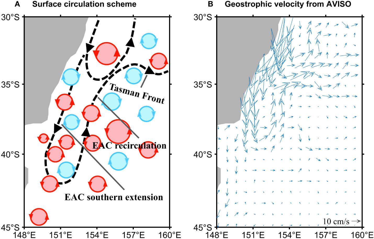
Figure 1 (A) A schematic diagram of identified current branches in the South Pacific subtropical Ocean modified from Oke et al. (2019). Schematic current branches (black dashed lines) are the EAC southern extension, the EAC recirculation, and the Tasman Front. The red and blue circles denote the mesoscale eddy field. (B) The distribution of climatological mean surface currents (arrow) in the EAC region (148°E-160°E, 30°S-45°S) from AVISO during January 1993-December 2019. The velocity vector represents the direction, and the length represents the magnitude of the velocity (10 cm s^-1).

The EAC has strong variability in the period of 90 to 150 days, accompanied by extensively active mesoscale eddy activities (Mata et al., 2006; Sloyan et al., 2016; Archer et al., 2017). Everett et al. (2012) showed that there was high eddy activities south of the EAC separation point at about 32°S off Australia's east coast detected from altimetry. Cetina-Heredia et al. (2019) drew the same conclusion using the particle trajectory data set from the eddy-resolving ocean general circulation model (OGCM) for the Earth Simulator (OFES) and the Connectivity Modeling System and pointed out that cyclonic eddies mainly prevailed in the north of 32°S, but anticyclonic eddies mainly prevailed in the EAC southern extension. The anticyclonic eddies is larger than cyclonic eddies (Cetina-Heredia et al., 2019) and about 88% of the EAC system eddies propagate westward, turning south when they encounter Australia's east shelf slope (Pilo et al., 2015). The eddy amplitude and rotational speed in the EAC eddy core region (31°S-38°S) are significantly higher than that of global (Everett et al., 2012). Compared with Kuroshio current [1.5 m s^-1, (Tseng et al., 2011)], the velocity of the EAC is relatively weak [-0.4 m s^-1, (Zilberman et al., 2018)]. The magnitude of EKE in the EAC region (Pilo et al., 2015; Li et al., 2021) is about 1/2 of that in the Kuroshio region (Miyazawa et al., 2004; Wang and Pierini, 2020), and EKE in the EAC region is still relatively strong. Archer et al. (2017) showed that EKE exhibited seasonal variations in both magnitude and variance with a maximum in summer and a minimum in the EAC region in winter. Using the 1/3°×1/3° spatial resolution satellite altimetry data from 1992 to 2002, Qiu and Chen (2004) reported that EKE in the EAC was high in summer and low in winter, while the maximum appeared in March and the minimum appeared in August.

The impact of forcing on mesoscale variability in the EAC region is revealed in previous studies. Bowen et al. (2005) suggested that mesoscale energy and energy propagation of the EAC were consistent with the variability generated by the current itself in the separated region, and were not forced by mesoscale signals propagating westward from the South Pacific basin. Mata et al. (2006) further indicated that the growth of mesoscale eddies was modulated by the local instability of flow using a global ocean model and altimetric data. Bull et al. (2017) found the EAC itself had high variability and was rarely affected by remote ocean variability using Nucleus for European Modelling of the ocean (NEMO).

Previous studies have also done some energetics analysis to study the dynamic mechanism of mesoscale eddy generation and shedding in the EAC region. Bowen et al. (2005) indicated that barotropic instability played a leading role in the process of driving eddy shedding in the area where the EAC mainstream separates from the coast. However, Mata et al. (2006) and Bull et al. (2017) implied both barotropic and baroclinic instabilities were highly active in the process of eddy shedding in the EAC region. Oliver et al. (2015) suggested the barotropic and baroclinic instability processes in the EAC southern extension region could drive the continuous growth and increase the life cycle of anticyclonic eddies. The generation and shedding of eddies in the EAC region are accompanied by extensively high EKE (Macdonald et al., 2016). It is worth noting that the above studies mainly analyzed energy conversion between mean available potential energy (MPE) to eddy potential energy (EPE) caused by baroclinic instability.

As for the energy source of EKE in the EAC region, Li et al. (2021) implied that barotropic instability dominated the variation of EKE on the interannual scale by comparing the magnitude of barotropic instability and baroclinic instability (EPE to EKE) using the ROMS data, but did not analyze the roles of the two instability processes on the seasonal variability of EKE in detail. So far, the main factors controlling the seasonal variability of the EKE and the underlying mechanism in the EAC region are still unclear.

In this paper, based on satellite altimeter observations and OFES simulation, the seasonal variation of EKE in the EAC region is studied in detail, and its dynamic mechanism is clarified to reveal the relationship between EKE and large-scale ocean circulation in the western boundary current region. This study could deepen our understanding of the mesoscale process with the large-scale circulation. This paper is organized as follows: Sect. 2 describes the satellite altimeter observations, OFES simulation, and oceanic Lorenz energy cycle method. Sect. 3 presents the seasonal cycle and dynamic processes of EKE. Sect. 4 is the summary and discussions.

2 Data and methods

2.1 Satellite observation of sea level anomalies from AVISO

The daily satellite observation of sea level anomalies (SLA) is derived from the Copernicus Marine Environment Monitoring Service (CMEMS, https://marine.copernicus.eu/) authenticated by Archiving Validation and Interpretation of Satellite Data in Oceanography (AVISO). The SLA product combines different altimeter measurements from Jason-3, Sentinel-3A, HY-2A, Saral/AltiKa, Cryosat-2, Jason-2, Jason-1, T/P, ENVISAT, GFO, ERS1/2. The spatial resolution is 0.25°×0.25°, the temporal resolution is 1 day, and the data span is from January 1 1993 to December 31 2020. AVISO can capture eddy activities in the EAC region (Oliver et al., 2015). In this study, using SLA, observed surface EKE can be readily calculated by:

$\begin{array}{ll}\text{EKE}=\frac{g^2}{2\text{f}}\left[{\left(\frac{\partial {\text{h}}^{\prime }}{\partial \text{x}}\right)}^2+{\left(\frac{\partial {\text{h}}^{\prime }}{\partial \text{y}}\right)}^2\right]& (1)\end{array}$

In Eq. (1), the Coriolis parameter f = 2Ωsin(φ), which depends on latitude φ and angular rate Ω, and $h^{\text{'}}$is sea level anomaly.

2.2 OGCM OFES

In this paper, OFES is used to study the vertical structure and dynamic mechanism of EKE. The flow field, temperature, and mesoscale eddy simulated by the OFES model are in good agreement with the observed results (e.g., transport (Wang et al., 2013; Cetina-Heredia et al., 2014), sea surface temperature (Wang et al., 2013), mesoscale eddy (Cetina-Heredia et al., 2019)). Thus, this model has the ability to reproduce the observed regional oceanographic features of the circulation in the EAC region. The OFES-CLIM run is initialized from the World Ocean Atlas 1998 (Boyer and Levitus, 1997) and is spun-up with the climatological monthly forcing from the National Centers for Environmental Prediction/National Center for Atmospheric Research (NCEP/NCAR) reanalysis (Kalnay et al., 1996) from 1950 to 1999 (Masumoto, 2004). After the 50 year spin-up integration, the OFES-NCEP run is forced by the daily atmospheric forcing of the NCEP/NCAR reanalysis from 1950. The OFES-QSCAT run is forced by the QuikSCAT wind data, taking the National Centers for Environmental Prediction run (NCEP-run) simulation output on 20 July 1999 as its initial condition. The OFES-QSCAT with a spatial resolution of 10 km is used in this study, which fully characterize mesoscale variability (Maltrud and McClean, 2005; von Storch et al., 2012; Chassignet and Xu, 2017).The spatial resolution is 0.1°×0.1°, the number of vertical levels is 54, and the time interval for the model archive is 3 days from 22 July 1999 to 30 October 2009.

3 Methods

The oceanic Lorenz energy cycle (LEC) is an effective method to assess EKE variation (Lorenz, 1955; Böning and Budich, 1992; Beckmann et al., 1994; Zhuang et al., 2010; Zu et al., 2013; Brum et al., 2017; Yan et al., 2019), and has been successfully applied to areas with strong ocean currents [e.g., the Kuroshio Extension (Yang and Liang, 2018); the Gulf Stream Region (Kang and Curchitser, 2015); the North Equatorial Countercurrent (Chen et al., 2015); the East Madagascar Current (Halo et al., 2014); the California current (Marchesiello et al., 2003); the Agulhas Return Current (Zhu et al., 2018); the South Indian Countercurrent (Zhang et al., 2020); EAC (Li et al., 2021)]. The energetics analysis is utilized to determine the energy sources of EKE. The EKE governing equation is as follows (Oey, 2008; von Storch et al., 2012; Su and Ingersoll, 2016):

$\begin{array}{ll}\frac{\partial \text{EKE}}{\partial \text{t}}=-\stackrel{⃑}{\text{v}}·\nabla \text{EKE-}\left[\overline{{\text{u}}^{\prime }{\text{u}}^{\prime }}\frac{\partial \overline{\text{u}}}{\partial \text{x}}+\overline{{\text{u}}^{\prime }{\text{v}}^{\prime }}\frac{\partial \overline{\text{u}}}{\partial \text{x}}+\overline{{\text{u}}^{\prime }{\text{v}}^{\prime }}\frac{\partial \overline{\text{u}}}{\partial \text{y}}+\overline{{\text{v}}^{\prime }{\text{v}}^{\prime }}\frac{\partial \overline{\text{v}}}{\partial \text{y}}\right]-\left(\overline{{\text{u}}^{\prime }{\text{w}}^{\prime }}\frac{\partial \overline{\text{u}}}{\partial \text{z}}+\overline{{\text{v}}^{\prime }{\text{w}}^{\prime }}\frac{\partial \overline{\text{v}}}{\partial \text{z}}\right)-\frac{\text{g}\overline{\text{ρ}\prime \text{w}\prime }}{{\text{ρ}}_0}+\frac{1}{{\text{ρ}}_0}\frac{\partial }{\partial \text{z}}\left(\overline{{\text{τ}}_{\text{x}}\text{'}u\text{'}(z=0)}+\overline{{\text{τ}}_{\text{y}}\text{'}\text{v}\text{'}(z=0)}\right)+\text{res}& (2)\end{array}$

$\begin{array}{ll}\text{BTR}=-\left[\overline{{\text{u}}^{\prime }{\text{u}}^{\prime }}\frac{\partial \overline{\text{u}}}{\partial \text{x}}+\overline{{\text{u}}^{\prime }{\text{v}}^{\prime }}\frac{\partial \overline{\text{u}}}{\partial \text{x}}+\overline{{\text{v}}^{\prime }{\text{v}}^{\prime }}\frac{\partial \overline{\text{u}}}{\partial \text{y}}+\overline{{\text{v}}^{\prime }{\text{v}}^{\prime }}\frac{\partial \overline{\text{v}}}{\partial \text{y}}\right]& (3)\end{array}$

$\begin{array}{ll}\text{BCR}=-\frac{\text{g}\overline{{\text{ρ}}^{\prime }{\text{w}}^{\prime }}}{{\text{ρ}}_0}& (4)\end{array}$

$\begin{array}{ll}{\text{BTR}}_{\text{v}}=-\left(\overline{{\text{u}}^{\prime }{\text{w}}^{\prime }}\frac{\partial \overline{\text{u}}}{\partial \text{z}}+\overline{{\text{v}}^{\prime }{\text{w}}^{\prime }}\frac{\partial \overline{\text{v}}}{\partial \text{z}}\right)& (5)\end{array}$

$\begin{array}{ll}\text{BTR}1=-\overline{{\text{u}}^{\prime }{\text{u}}^{\prime }}\frac{\partial \overline{\text{u}}}{\partial \text{x}}& (6)\end{array}$

$\begin{array}{ll}\text{BTR}2=-\overline{{\text{u}}^{\prime }{\text{v}}^{\prime }}\frac{\partial \overline{\text{v}}}{\partial \text{x}}& (7)\end{array}$

$\begin{array}{ll}\text{BTR}3=-\overline{{\text{u}}^{\prime }{\text{v}}^{\prime }}\frac{\partial \overline{\text{u}}}{\partial \text{y}}& (8)\end{array}$

$\begin{array}{ll}\text{BTR}4=-\overline{{\text{v}}^{\prime }{\text{v}}^{\prime }}\frac{\partial \overline{\text{v}}}{\partial \text{y}}& (9)\end{array}$

$\overline{u}$ and $\overline{v}$ are zonal and meridional components of background currents with the time scale longer than 150 days, and $u\text{'}$ and $v\text{'}$ are high-frequency perturbations of zonal and meridional components with the time scale shorter than 150 days, consistent with previous studies in the EAC (Mata et al., 2006; Sloyan et al., 2016). Similarly, $\rho \text{'}$ and $w\text{'}$ are the perturbations of potential density and vertical velocity, respectively. Potential density ρ₀ = 1025kg m^-3. The gravitational constant g =9.8N kg^-1. The density ρ is calculated from the potential temperature (T) and salinity (S).

Eq. (2) is the EKE balance equation, which describes the EKE balances at steady state. $\frac{\partial \text{EKE}}{\partial t}$ is the temporal change rate (time trend) of EKE; $-\stackrel{\rightharpoonup }{\text{v}}·\nabla \text{EKE}$ means the redistribution rate of EKE through advection; the barotropic conversion rate (BTR) in Eq.(3) represents the EKE is produced by the shear and Reynolds stress of the flow. BTR serves as an indicator of energy transfer between mean kinetic energy (MKE) and EKE via barotropic instability and measures the strength of barotropic instability. Positive BTR indicates that energy is transferred from MKE to EKE (Orr, 1907) and the energy of the background circulation is transferred to eddies via barotropic instability (McWilliams, 2006), and negative BTR indicates that energy of background circulation is transferred to eddies. BCR in Eq.(4) serves as an indicator of energy transfer between EPE and EKE via baroclinic instability. The change in potential energy is performed by turbulent buoyancy forces on the vertical stratification. Positive BCR indicates that energy is transferred from EPE to EKE via baroclinic instability (Cushman-Roisin and Jean-Marie, 2011; Gula et al., 2015; Torres et al., 2018; Yu et al., 2019). the vertical barotropic conversion rate (BTR_v) in Eq.(5) represents the energy is transferred due to small-scale shear instability. Since the vertical velocity w is much smaller than the horizontal velocity, it can be ignored. $\frac{1}{{\text{ρ}}_0}\frac{\partial }{\partial \text{z}}\left(\overline{{\text{τ}}_{\text{x}}\text{'}u\text{'}(z=0)}+\overline{{\text{τ}}_{\text{y}}\text{'}\text{v}\text{'}(z=0)}\right)$ represents EKE is generated by the wind work and res is the energy dissipation, which can be ignored (Oey, 2008; von Storch et al., 2012). For detailed derivation and further discussion of the LEC, please refer to (Böning and Budich, 1992; Rubio et al., 2009; Kang and Curchitser, 2015).

4 Results

4.1 Seasonal variability of EKE

The distribution of surface mean EKE from satellite altimeter observations in the EAC is shown in Figure 2A. High EKE (>500 cm² s^-²) exists along Australia’s east coast, and is mainly concentrated in the shear-region between the EAC southern extension and the EAC recirculation and extends to Tasmania, consistent with previous observations (Pilo et al., 2015; Li et al., 2021). There is a high EKE core at around 153°E, 35°S from observation data. The EKE averaged over the upper 300 m layer from OFES from July 1999 to October 2009 also shows a high core at around 153°E, 35°S (Figure 2B). Thus, the EKE averaged over the upper 300 m layer derived from the OFES simulation has similar spatial distribution and magnitude as the observed surface EKE from AVISO (Figures 2A, B). The EKE from OFES in south of 40°S is stronger than that from AVISO, which maybe come from overestimated modeled current (S1 in appendix) contrasting with that from AVISO (Figure 1B). In addition, the observed surface EKE averaged in 148°E-160°E, 30°S-45°S reaches the maximum (465±89 cm² s^-²) in February, then gradually falls until it reaches the minimum (334±48 cm² s^-²) in August, and then rises from September to January of the next year, with mean EKE value of 392 cm² s^-² (Figure 3, red solid line). The simulated seasonal variation of surface EKE (Figure 3, blue solid line) and averaged EKE over the upper 300 m layer (Figure 3, blue dash line) is strongest in February and weakest in July. EKE from satellite altimeter observations and OFES exhibits similar seasonal variations. Therefore, the OFES still provides a reasonable simulation of the spatial distribution and seasonal cycle of EKE in the EAC region.

FIGURE 2

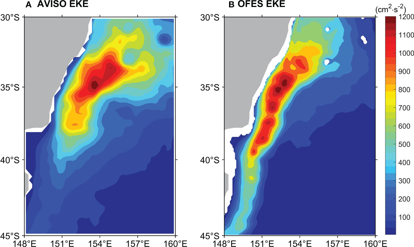
Figure 2 Climatological mean eddy kinetic energy (EKE, Unit: cm² s^-²) calculated from the SLA data from (A) AVISO during January 1993-December 2019 and (B) OFES (0-300m) during July 1999-October 2009. EKE is calculated from Eq. (1).

FIGURE 3

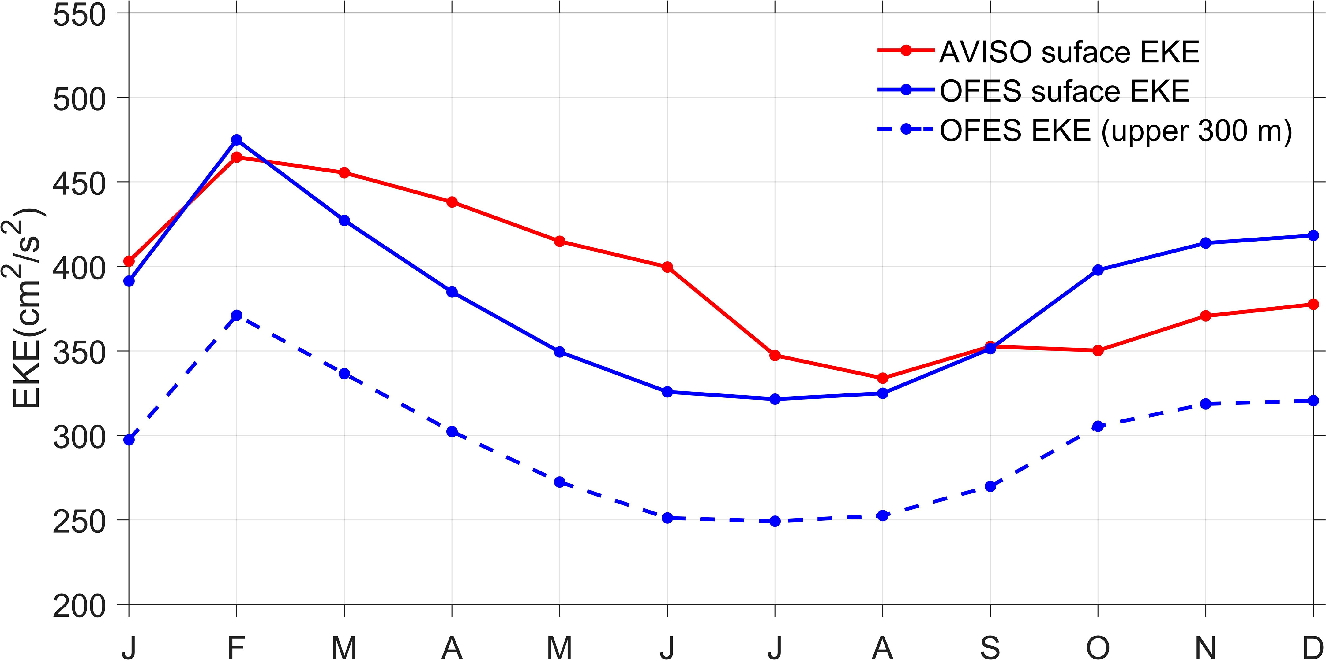
Figure 3 Monthly EKE time series in the EAC region (148°E-160°E, 30°S-45°S) calculated from AVISO during January 1993-December 2019 and from OFES during July 1999-October 2009. Red solid line and blue solid line represent surface EKE from AVISO and OFES, blue dash line represents averaged EKE over the upper 300 m layer from OFES.

The vertical structure of the EKE is studied using the OFES model output. The regional mean EKE at different depths is depicted as E(t,z) following Chen et al. (2015). The $\frac{E(t,z)}{E(t,0)}$ indicates mean EKE normalized with the surface value is a function of depth. The black line shows that EKE drops rapidly with increasing depth and the mean EKE at 300 m is only approximately 35% of the surface value in the EAC region (Figure 4). The C(z) indicates the coherence value of EKE time series at different depths relative to the surface EKE, defined by the following equation:

$\begin{array}{ll}C(z\text{)}\equiv 1-\frac{{\langle \left[E(t,z)-r(z)E(t,0)\right]}^2\rangle }{\langle E^2(t,z)\rangle }& (10)\end{array}$

FIGURE 4

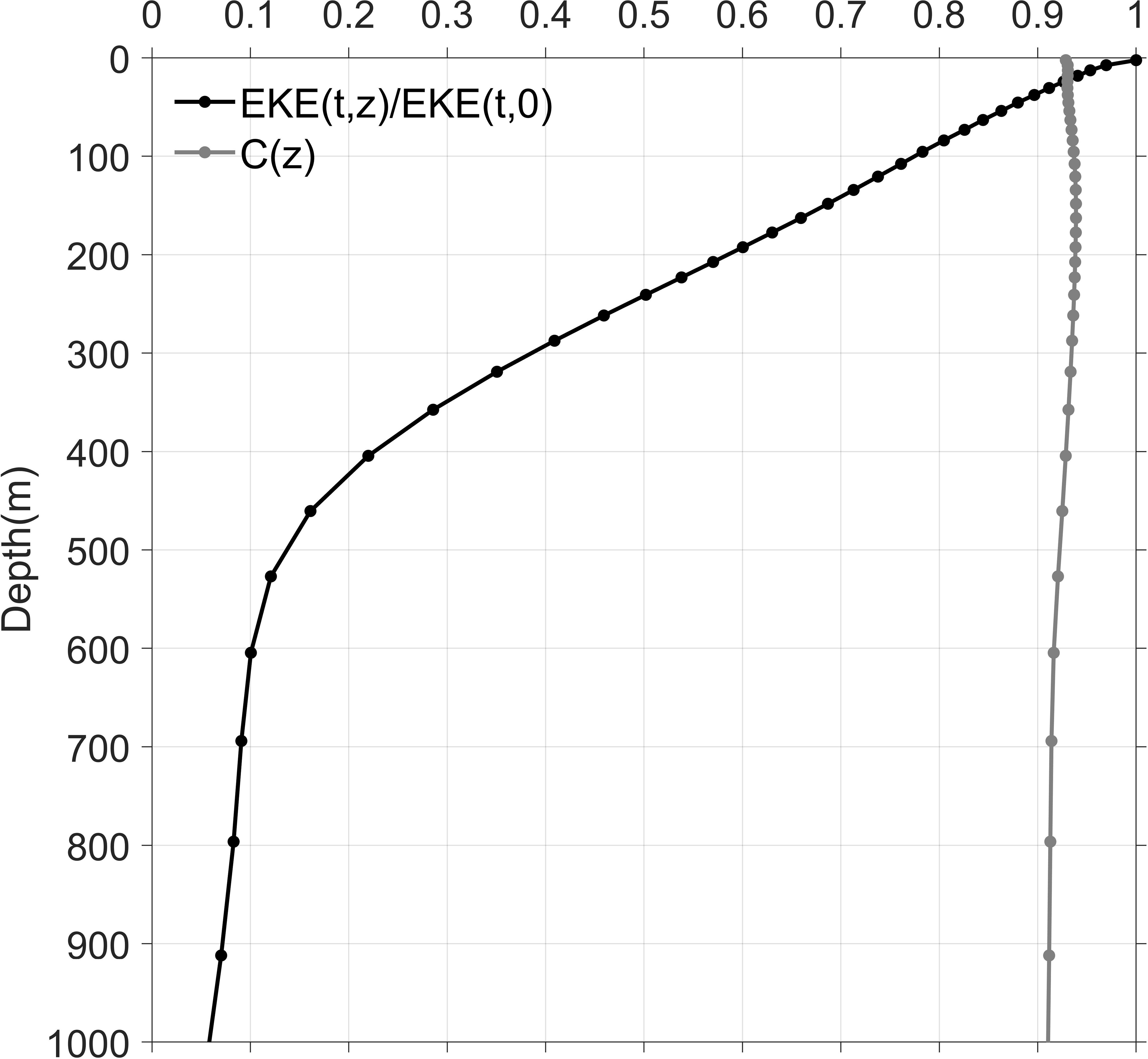
Figure 4 Black line: EKE averaged in 148°E-160°E, 30°S-45°S as a function of depth from OFES; the standardized EKE level as a function of depth: $\frac{E(t,z)}{E(t,0)}$. Gray line: the EKE coherence level as a function of depth relative to surface EKE: C(z), and C(z) is defined in Eq. (10).

where r(z) is a regression coefficient, r(z) ≡ ⟨E(t,z)E(t,0)/E²(t,0)⟩. Physically, C(z) indicates the ratio of E(t,z) variance that is coherent in respect of E(t,0). C(z) exceeds 0.9 at all depths indicates that the temporal variability of EKE in the upper 300 m layer is similar to the surface (Figure 4). Considering the vertical distribution of EKE, the EKE, BTR, BCR, and current velocity are averaged over the upper 300 m layer to study the dynamic mechanism using the OFES simulation in the following.

4.2 Seasonal variability of BTR and BCR

Figure 5 shows the monthly spatial distribution of EKE averaged over the upper 300 m layer obtained by the OFES model from July 1999 to October 2009. High EKE always appears in the shear-region between the EAC southern extension and the EAC recirculation along Australia’s east coast. The high EKE core near 151°E, 32°S in August (Figure 5H) is gradually strengthened and moves southward until it appears at 151°E, 38°S in February (Figure 5B). EKE is strongest in summer (Figures 5L, A, B) and weakest (Figures 5F–H) in winter in the shear region. Meanwhile, the spatial distribution of EKE from AVISO is similar to that of OFES (S2 in Appendix).

FIGURE 5

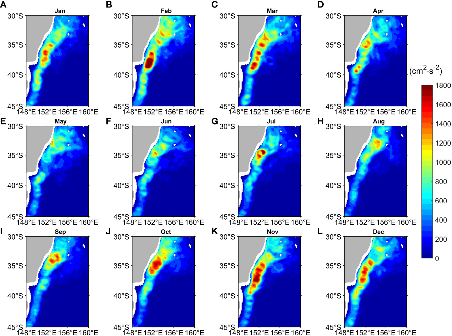
Figure 5 Monthly mean EKE distribution averaged over the upper 300 m layer from OFES during July 1999-October 2009 for (A) January, (B) February, (C) March, (D) April, (E) May, (F) June, (G) July, (H) August, (I) September, (J) October, (K) November and (L) December.

MKE and EPE can be transferred to EKE via barotropic and baroclinic instabilities, respectively (Halo et al., 2014; Chen et al., 2015; Kang and Curchitser, 2015; Yang and Liang, 2018; Zhu et al., 2018; Zhang et al., 2020; Li et al., 2021). Next, we will ascertain the energy source of EKE on the seasonal scale in the region.

The BTR in the EAC region exhibits a mixed positive-negative pattern (Figure 6). The high positive and negative BTR is mainly concentrated in the shear-region corresponding to the high EKE (Figures 5, 6), consistent with previous studies (Bowen et al., 2005; Mata et al., 2006; Li et al., 2021). It implies that the energy conversion between the mean flow and the eddy field is active via barotropic instability. High negative BTR values indicate that inverse energy cascades frequently appear in the shear-region, and eddy energy transfer toward MKE may play an important role in influencing mean flow in the shear-region. The positive and negative values appear alternately along the EAC southern extension and EAC recirculation, and show significant along-stream variability (Figure 6), which is similar to the spatial pattern near the Charleston Bump in the Gulf Stream Region (Kang and Curchitser, 2015).

FIGURE 6

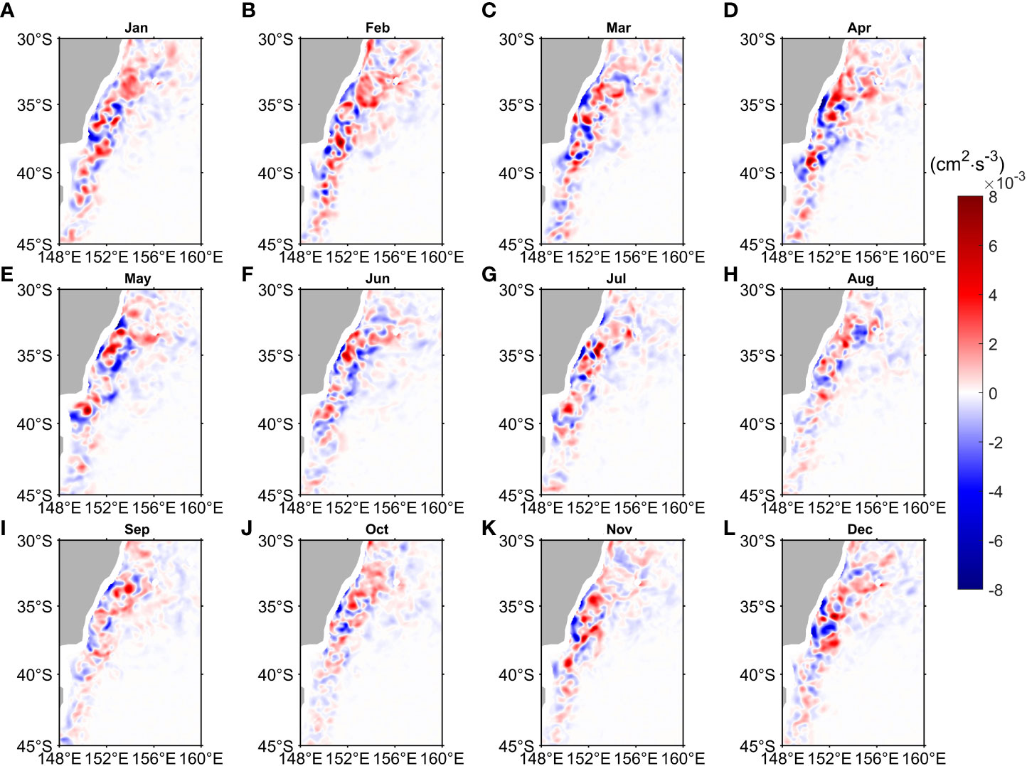
Figure 6 Monthly mean barotropic conversion rate (BTR, Unit: cm² s^-3) distribution averaged over the upper 300 m layer from OFES during July 1999-October 2009 for (A) January, (B) February, (C) March, (D) April, (E) May, (F) June, (G) July, (H) August, (I) September, (J) October, (K) November and (L) December. BTR is defined in Eq. (3).

The transfers of MKE→EKE and EKE→MKE are highly energetic in each season. The positive BTR is strong in summer (Figures 6L, A, B) and weak in winter (Figures 6F–H), suggesting that energy transferred from MKE to EKE is an important energy source for eddies via barotropic instability in summer. BTR at the EAC main separation point (31°S-32°S) is not as high as BTR south of 32°S, indicating that the eastward Tasman Front is not the main factor for barotropic instability (Figure 6). In addition, the vertical profile of BTR averaged between 30°S and 45°S shows that conversion between MKE and EKE is mainly confined within the upper depths (0-300 m) and is consistent in the vertical direction (S3 in Appendix).

The spatial distribution of BCR is quite different from that of BTR in the EAC region. It is noteworthy that the magnitude of BCR is 1/8 of BTR (Figures 6, 7). In each season BCR is positive in most parts of the shear-region suggesting that energy transfer from EPE to EKE via baroclinic instability is active in this region. The negative BCR mainly exists along coast (32°S-38°S) and appears at 155°E, 33°S, and maybe results from the influence of the topography. Meanwhile, the positive BCR is strong in winter (Figures 7F, G, H), and in other seasons it is relatively weak. In addition, the vertical profile of BCR averaged between 30°S and 45°S demonstrates that the conversion of EPE between EKE is mainly confined within the upper depths (0-300 m). BCR is mainly positive, especially in winter suggesting that EPE tends to convert to EKE via baroclinic instability and more energy is converted to EKE in winter (S4 in Appendix).

FIGURE 7

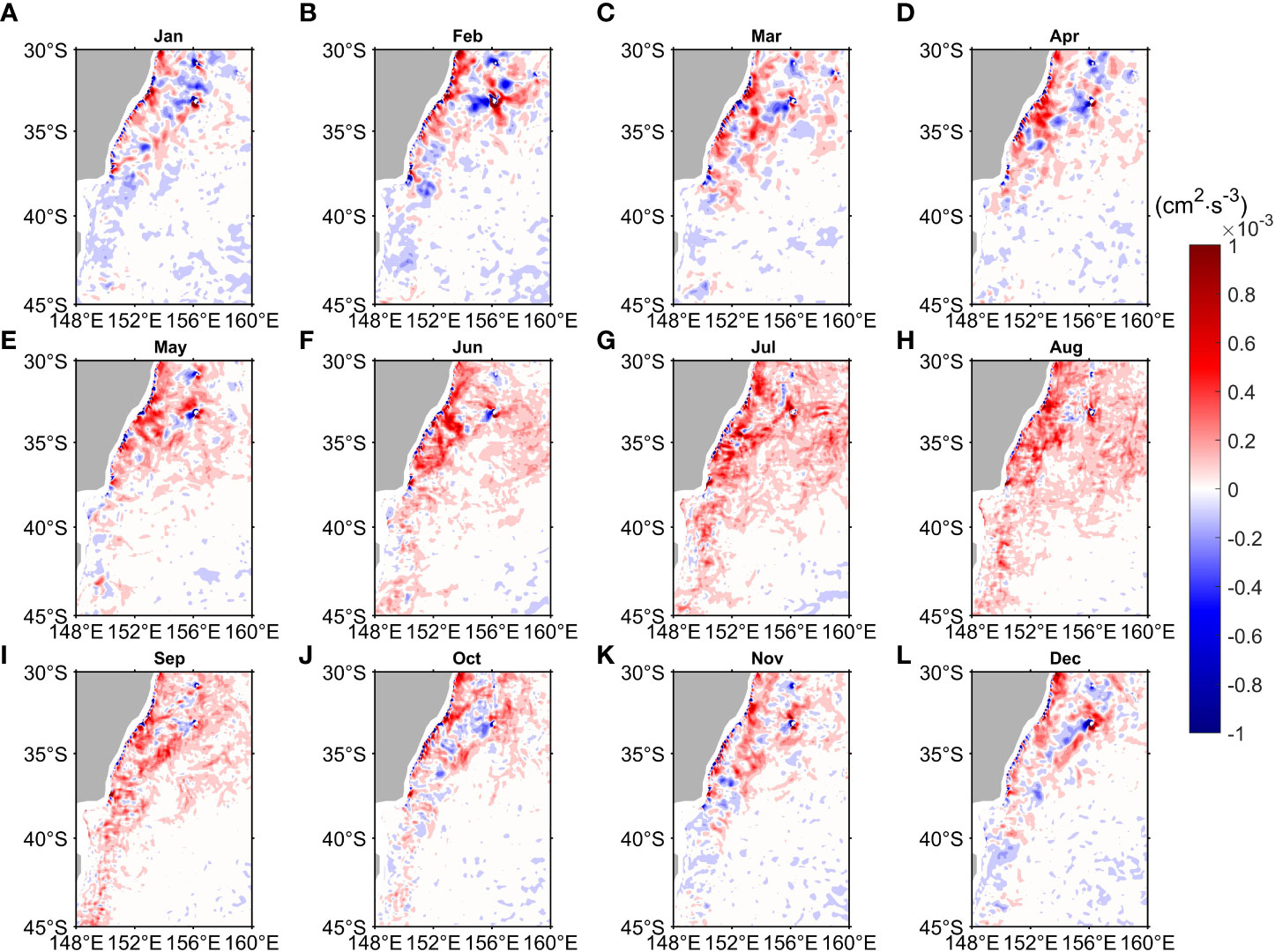
Figure 7 Monthly mean baroclinic conversion rate (BCR, Unit: cm² s^-3) distribution averaged over the upper 300 m layer from OFES during July 1999-October 2009 for (A) January, (B) February, (C) March, (D) April, (E) May, (F) June, (G) July, (H) August, (I) September, (J) October, (K) November and (L) December. BCR is defined in Eq. (4).

To quantify the energy source of EKE in the EAC, Figure 8 depicts the monthly time series of the horizontal mean $\frac{\partial \text{EKE}}{\partial t}$、BCR、BTR, and the sum of BTR and BCR (BCR+BTR) in the EAC (148°E-160°E, 30°S-45°S). The $\frac{\partial \text{EKE}}{\partial t}$ (blue line) is positive in February-March and September-December with an increase in EKE, while it is negative in other months with a decrease in EKE, presenting a double-peak structure in general. BCR+BTR (black line) are mainly positive confirming that both barotropic and baroclinic instabilities are the energy sources for EKE in the EAC region in climatological mean state, thus contributing to the intensive eddy activities in the EAC region. BTR (red line) reaches the maximum (1.30×10^-4 cm² s^-3) in February and reaches the minimum (1.55×10^-5 cm² s^-3) in June. The maximum (1.28×10^-4 cm² s^-3) of BCR (gray line) appears in July and the minimum (3.17×10^-5 cm² s^-3) appears in January. The main sources of EKE are the barotropic instability in summer and the baroclinic instability in winter, and the barotropic and baroclinic instabilities are equally important in other months. Because the order of magnitude of the spatial distribution of BCR is smaller than that of BTR, Li et al. (2021) believed that EKE in the EAC region on the interannual scale was mainly governed by barotropic instability. However, the spatial mean of BCR is comparable to that of BTR (Figure 8), because the positive and negative values of BTR are mostly offset (Figure 6). BCR+BTR is consistent with $\frac{\partial \text{EKE}}{\partial t}$ on the seasonal scales (Figure 8), suggesting both barotropic and baroclinic instabilities play an important role in modulating the seasonal variability of EKE.

FIGURE 8

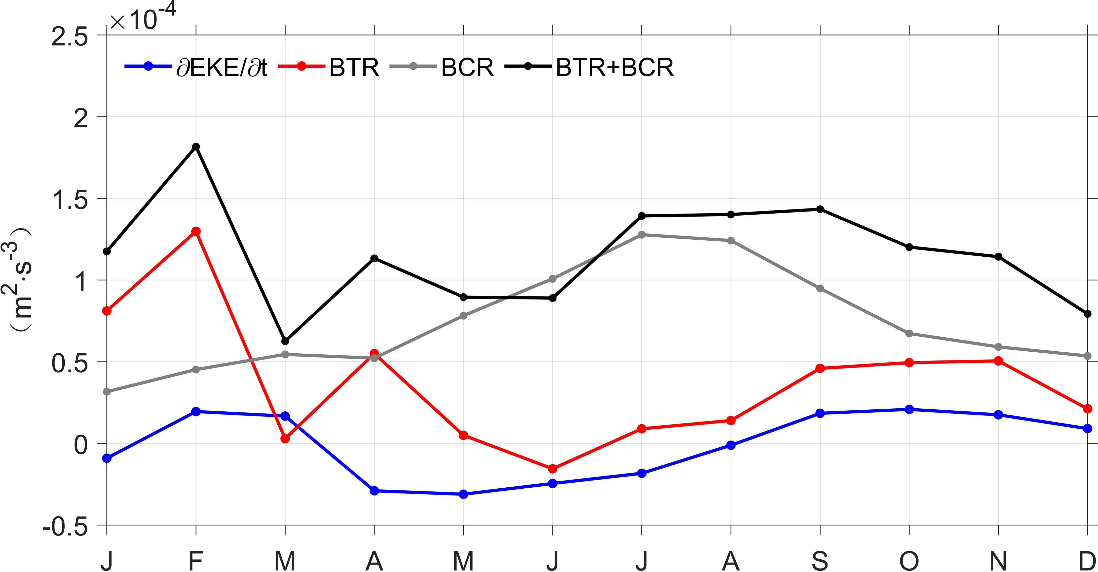
Figure 8 Seasonal variations of mean EKE trend (blue line), BTR (red line), BCR (gray line), and BTR+BCR (black line) averaged over the upper 300 m layer from OFES during July 1999-October 2009 in the EAC region (148°E-160°E, 30°S-45°S).

4.3 Mechanism of the seasonal variability of EKE

Since the enhancement of EKE in the EAC is mainly due to the strong barotropic instability in summer (Figure 8), we will study the main factors influencing BTR. Energetics analysis of Eq. (3) illustrates that BTR is closely related to the horizontal shear of flows. The seasonal variations of BTR1-BTR4 are quantitatively calculated to study the contribution of each term to BTR (Figure 9). BTR2 (green solid line) reaches its maximum (4.57×10^-4 cm² s^-3) in February and its minimum (1.73×10^-4 cm² s^-3) in August. Contrasting with mainly positive values of BTR (red solid line), both BTR1 (blue dash line) and BTR3 (black dash line) are negative each month, and out of phase with BTR. The amplitude of BTR4 is smaller than BTR2, and seasonal variability of BTR4 is not obvious and out of phase with BTR. Therefore, the influence of BTR4 can be ignored. Overall, the seasonal variation of BTR2 is consistent with that of BTR (Figure 8, 9), and the amplitude of BTR2 plays a dominant role in the four terms, suggesting that BTR2 makes the main contribution to BTR.

FIGURE 9

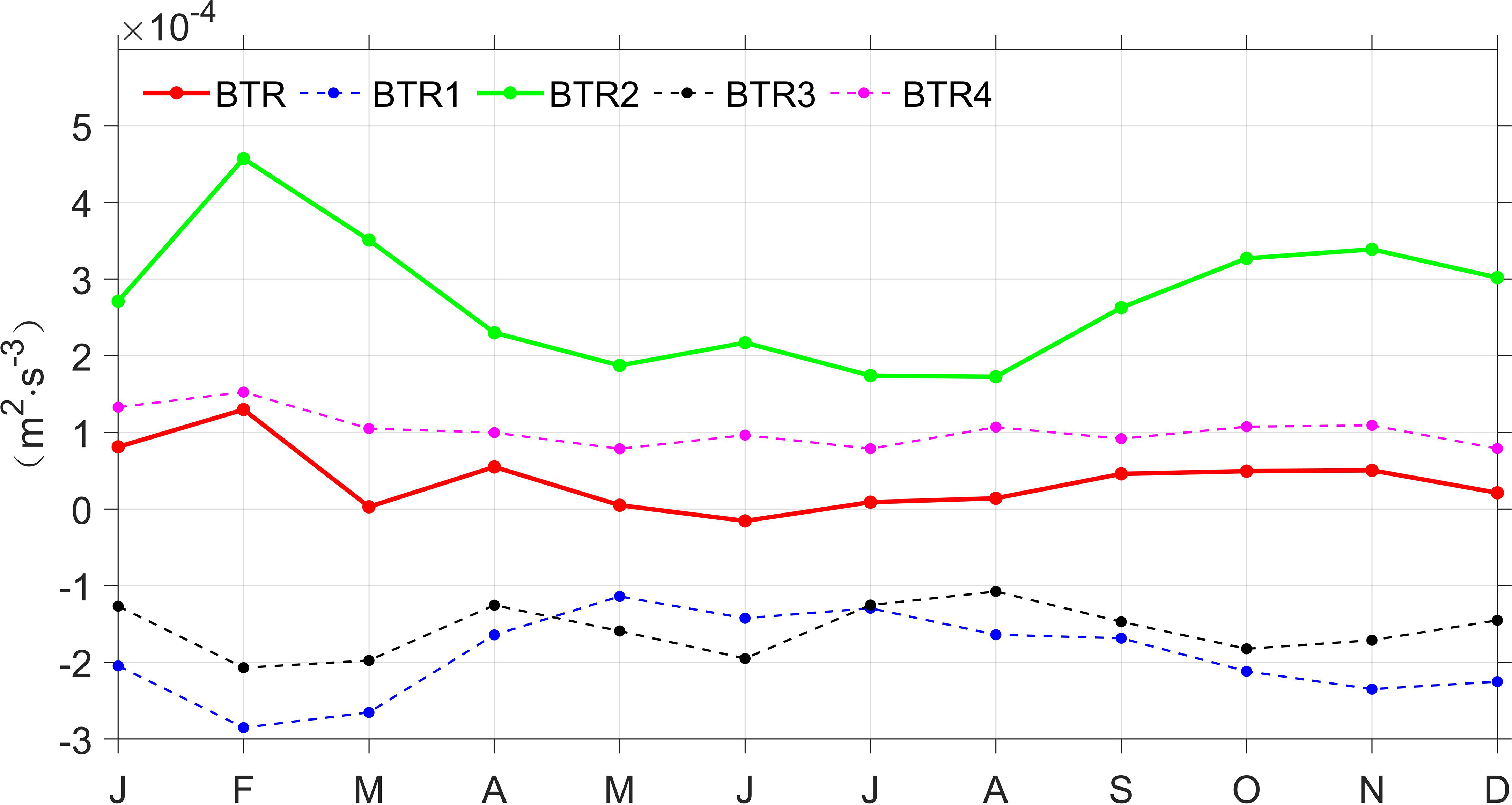
Figure 9 Seasonal variations of spatial mean BTR (red solid line), BTR1 (blue dash line), BTR2 (green solid line), BTR3 (black dash line), and BTR4 (magenta dash line) averaged over the upper 300 m layer from OFES during July 1999-October 2009 in the EAC region (148°E-160°E, 30°S-45°S).

Because the BTR stands for energy transfer between MKE of background circulation and EKE via barotropic instability (McWilliams, 2006), and previous studies in the Celebes Sea (Yang et al., 2020) and in the North Equatorial Countercurrent of Western Pacific (Chen et al., 2015) show that variation of EKE is governed by barotropic instability of the background circulation. Next, we will analyze the role of background circulation in the variation of BTR. Considering that BTR2 partly represents the zonal gradient of low-pass filtered meridional velocity ($\frac{\partial \overline{v}}{\partial x}$) as shown in Eq. (7), and the location of high BTR corresponds to the shear-region between the poleward EAC southern extension and the equatorward EAC recirculation (Figures 1, 6), we should verify the role of the zonal gradient of meridional velocity in controlling the variation of BTR2 and BTR. The seasonal variability of $\frac{\partial \overline{v}}{\partial x}$ along 38°S is shown in Figure 10. The location of maximum southward velocity (the current axis of the EAC southern extension) is near 150.5°E, the location of maximum northward velocity (the current axis of the EAC recirculation) is near 152°E, and maximum value of $\frac{\partial \overline{v}}{\partial x}$ is near 151.5°E. The $\frac{\partial \overline{v}}{\partial x}$ is strongest in February and weakest in July, consistent with the seasonal variation of BTR2 and BTR (Figures 8–10), confirming that zonal gradient of meridional velocity between the EAC southern extension and the EAC recirculation makes the main contribution to barotropic instability.

FIGURE 10

Figure 10 Seasonal variability of $\frac{\partial \overline{v}}{\partial x}$ (shaded color), and $\overline{v}$ (contour with 5 intervals, units: cm s^-1) along 38°S averaged over the upper 300 m layer from OFES during July 1999-October 2009. Solid (dash) lines represent positive (negative) meridional velocity.

The minimum velocity between 150°E and 151.5°E and maximum velocity between 151.5°E and 152.5°E averaged over the upper 300 m along 38°S stand for the poleward EAC southern extension (Vmin) and the equatorward EAC recirculation (Vmax), respectively. And the difference between them (Vmin-Vmax) represents the zonal shear of meridional velocities of the EAC southern extension and the EAC recirculation. Both absolute values of Vmin and Vmax have the maximum in February and the minimum in July (Figure 11). The seasonal variation of the EAC southern extension (black line) and the EAC recirculation (blue line) is synchronous, consistent with previous studies indicating that the EAC southern extension is negatively correlated with the EAC recirculation (Zilberman et al., 2014; Sloyan and O'Kane, 2015). The Vmin-Vmax (red line) is strongest (-95.18 cm s^-1) in February and weakest (-19.11 cm s^-1) in July. The seasonal variation of zonal shear of meridional velocities is controlled by the synchronously seasonal varying poleward EAC southern extension and equatorward EAC recirculation (Figure 11).

FIGURE 11

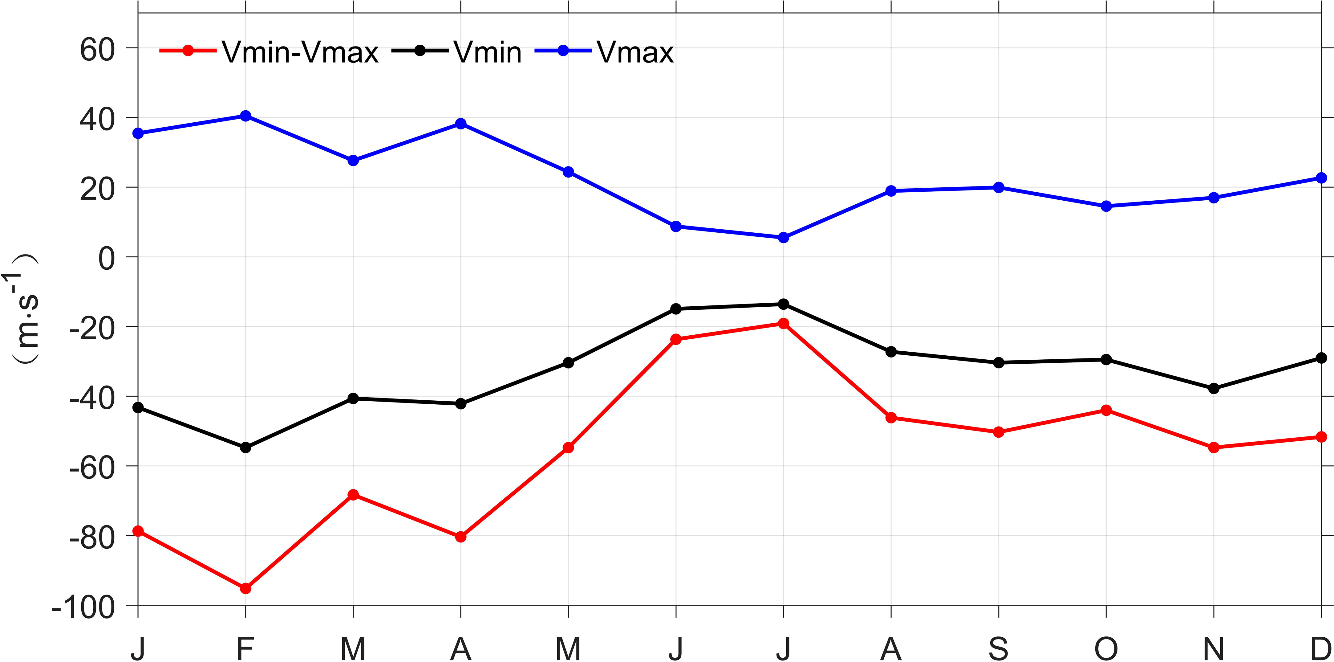
Figure 11 Seasonal variation of velocity of the EAC southern extension (Vmin, units: cm s^-1), the EAC recirculation (Vmax, units: cm s^-1), and the difference between the two currents (Vmin-Vmax, red line, units: cm s^-1) along 38°S. The black line is Vmin, the blue line is the Vmax, and the red line is Vmin-Vmax averaged over the upper 300 m layer from OFES during July 1999-October 2009.

The zonal shear of meridional currents matches well with the seasonal variation in EKE (Figures 3, 11), suggesting a synchronous phase relationship between the EKE and zonal shear of meridional currents. In other words, due to the dominant meridional circulation in this region, when the EAC southern extension and the EAC recirculation are strong, the zonal shear between the currents will be reinforced, and barotropic instability is enhanced, and it contributes to high EKE transferred from MKE. The result is consistent with other studies suggesting that horizontal shear of highly energetic flow tends to support EKE generation via barotropic instability (Chen et al., 2016; Zhan et al., 2016).

Furthermore, we examine the relationship between currents and SLA, the seasonal variation of SLA is obtained from AVISO from January 1999 to December 2009. In the EAC region, SLA is positive (negative) in summer (winter) (Figure 12), and the poleward EAC southern extension and the equatorward EAC recirculation are strengthened (weakened) due to geostrophic equilibrium (Figure 11). Then, the zonal shear of meridional currents is strengthened (weakened), and the EKE is strong (weak) via barotropic instability (Figures 3, 11). The SLA could influence the shear strength of upper ocean currents thus dynamically affecting the EKE. In addition, mesoscale eddies can be approximatively identified with SLA. Li et al. (2021) revealed there are more anticyclonic eddies than cyclonic eddies in the period of high EKE in the EAC on the interannual scale. Similarly, the anticyclonic circulation pattern of the poleward EAC southern extension and the equatorward EAC recirculation is more conducive to the formation of anticyclonic eddies in summer with high EKE (Figures 12L, A, B), and can explain the phenomenon found by Cetina-Heredia et al. (2019) that anticyclonic eddies are more common in EAC southern extension.

FIGURE 12

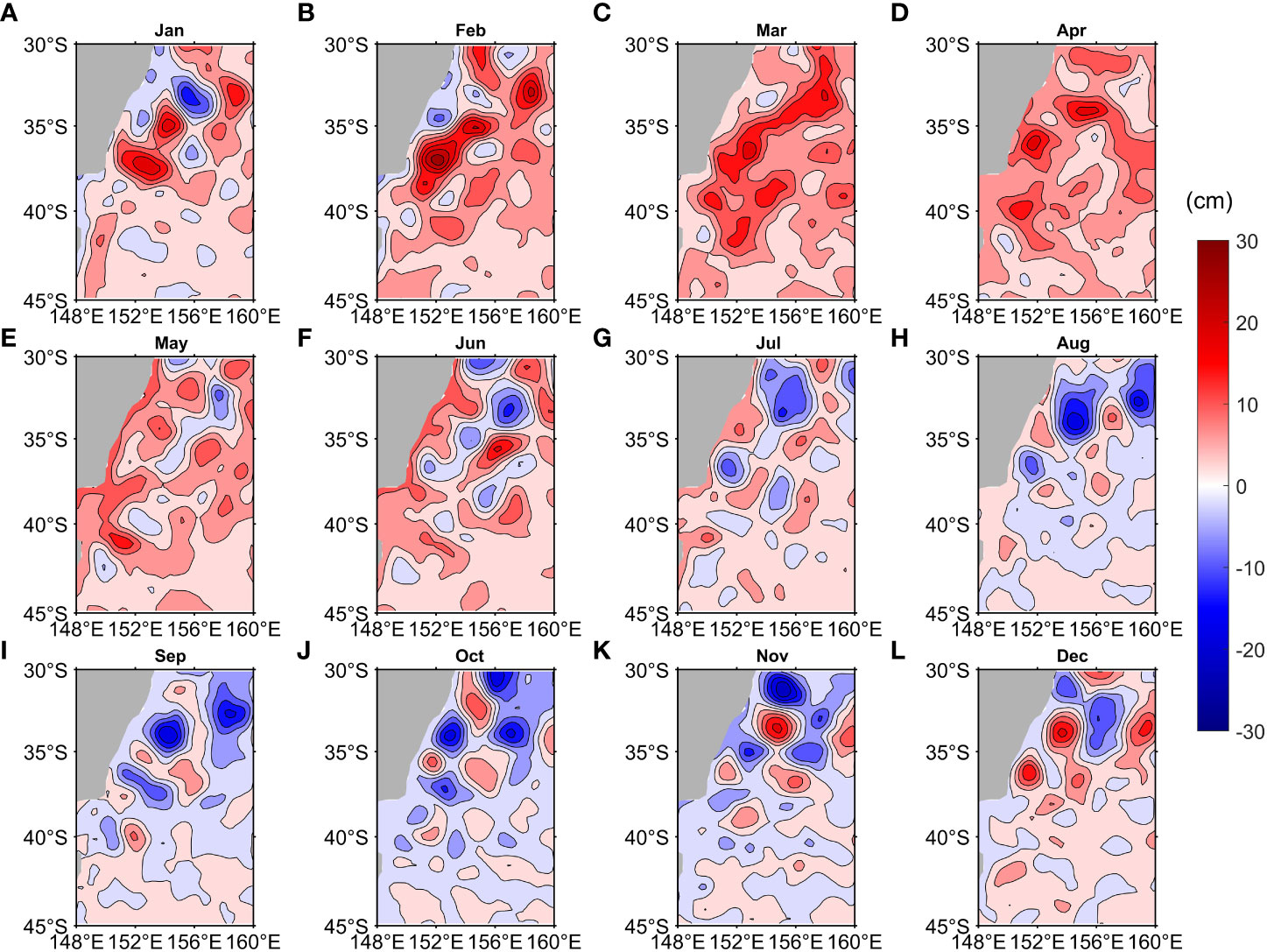
Figure 12 Monthly mean Sea Level Anomalies (SLA, Unit: cm) distribution from AVISO during January 1999-December 2009 for (A) January, (B) February, (C) March, (D) April, (E) May, (F) June, (G) July, (H) August, (I) September, (J) October, (K) November and (L) December.

Figure 13 demonstrates the zonal distributions of temperature and velocity in the upper 300 m from the OFES model along 38°S. The zonal temperature gradient is positive on the west side of 152°E and negative on the east side, and the temperature trough reaches the deepest near 152°E in each season. The EAC southern extension (blue shaded color) and the EAC recirculation (red shaded color) are trapped above the west and east of the temperature trough, respectively (Figure 13). The velocity direction changes little with the increase of depth (S1 in appendix), which is consistent with the study of Mata et al. (2006) through satellite altimeter observations and current meter array. Here, the zonal mean depth of 15°C isotherm between 151°E-152°E along 38°S stands for the depth of temperature trough for quantitative analysis and is defined as D₁₅. The D₁₅ reaches the deepest point (305.58 m) in February and reaches the shallowest point (221.81 m) in July (Figure 14). The D₁₅ is high (low) in summer (winter), which is corresponding to more (less) anticyclonic eddies with positive (negative) SLA (Figure 12). Under geostrophic equilibrium, the poleward EAC southern extension and the equatorward EAC recirculation are strengthened (weakened), thus the variations of zonal shear and BTR have a good corresponding relationship with the D₁₅ (Figures 8, 11, 14).

FIGURE 13

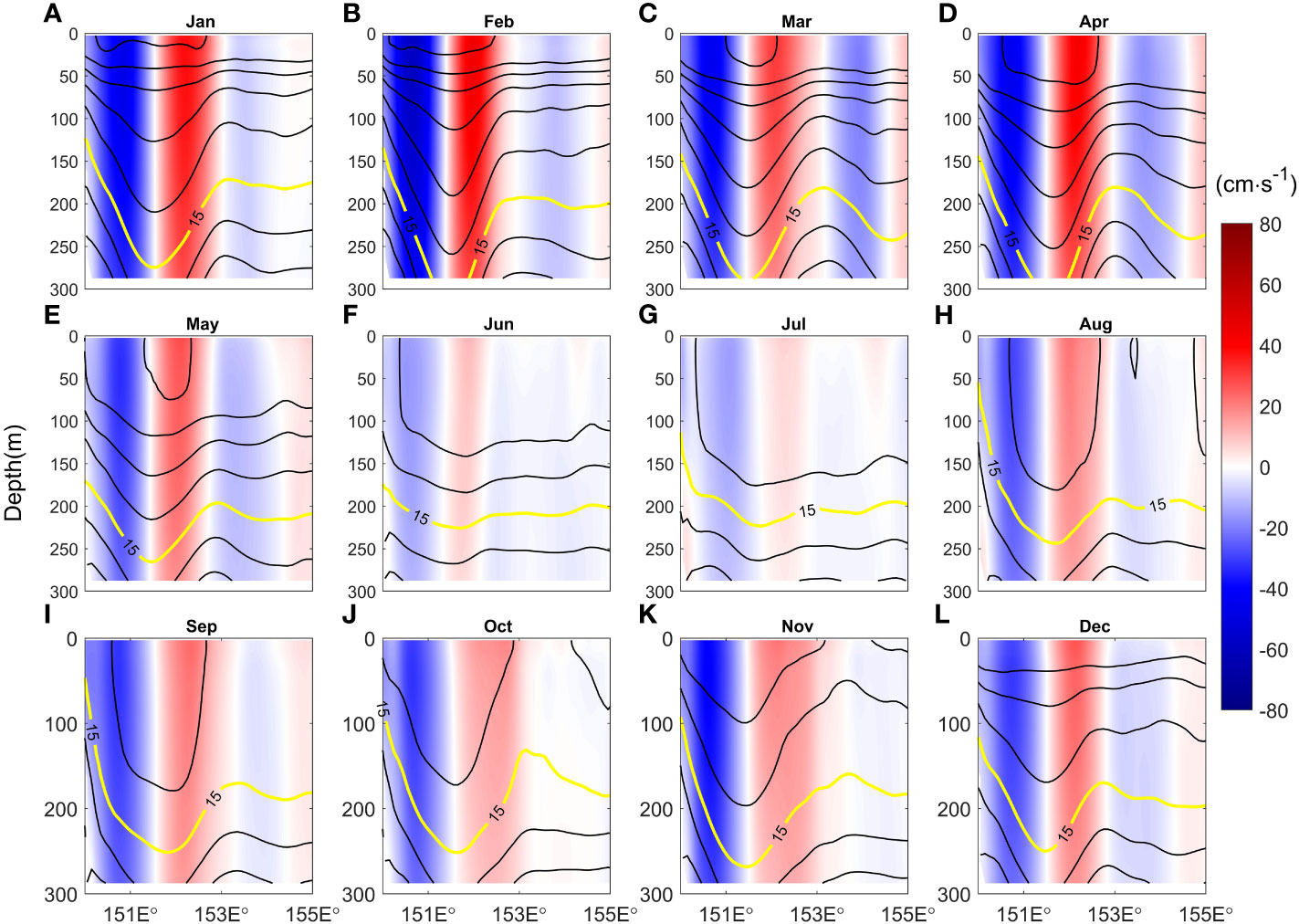
Figure 13 Zonal distributions of temperature (contour with 1 interval, units: °C) and velocity (shaded color, units: cm s^-1) in the upper 300 m along 38°S from OFES during July 1999-October 2009 for (A) January, (B) February, (C) March, (D) April, (E) May, (E) June, (G) July, (H) August, (I) September, (J) October, (K) November and (L) December.

FIGURE 14

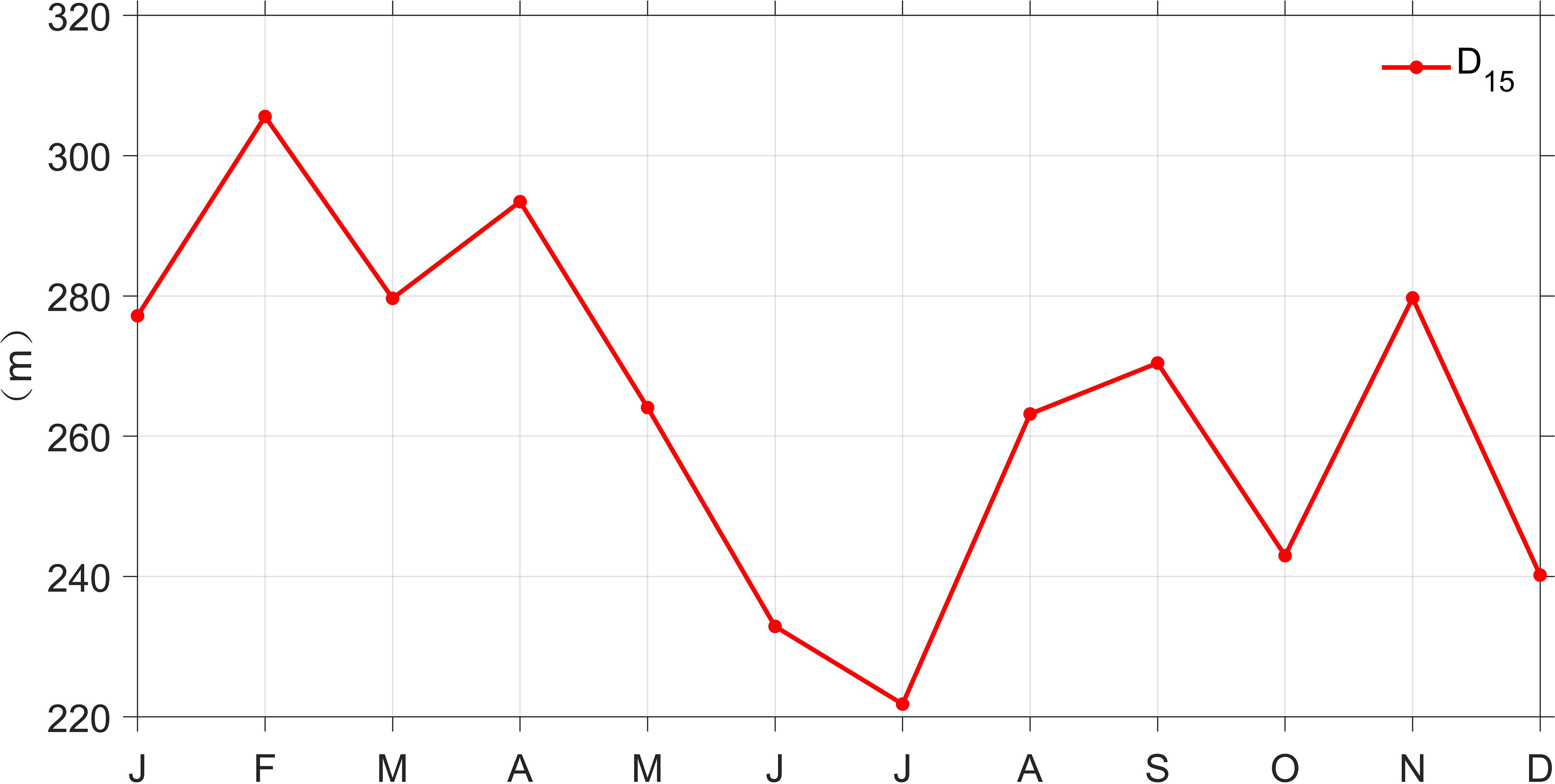
Figure 14 Seasonal variation of D₁₅ along 38°S from OFES during July 1999-October 2009.

5 Summary and discussions

The seasonal cycle and dynamic mechanism of EKE in the EAC region are studied using satellite altimeter observations and high-resolution OFES-QSCAT model data. The high EKE is mainly concentrated in the shear-region of the poleward EAC southern extension and the equatorward EAC recirculation along Australia’s east coast and is confined within the upper ocean (0-300 m). EKE displays a distinct seasonal cycle characteristic with a maximum value (465 cm² s^-²) in February and a minimum value (334 cm² s^-²) in August. The energy conversion terms are quantitatively analyzed, indicating that the seasonal variability of EKE is modulated by the mixed instabilities. Both barotropic and baroclinic instabilities are the energy sources of EKE in the EAC region, and barotropic instability dominates high EKE in summer and baroclinic instability influences EKE in winter. The variation of barotropic instability is dominated by zonal shear associated with synchronously-varying the poleward EAC southern extension and the equatorward EAC recirculation modulated by local SLA. In the EAC region, the local SLA is positive (negative) in summer (winter), then the poleward EAC southern extension and the equatorward EAC recirculation are synchronously strengthened (weakened) due to geostrophic equilibrium. And barotropic instability of the zonal shear between the poleward EAC southern extension and the equatorward EAC recirculation is enhanced (slackened), thus leading to high (low) EKE transferred from MKE.

Mata et al. (2006) have discovered the SLA propagates southward along the east Australian continental slope and it may account for the seasonal variation of local SLA in the shear-region. Besides, baroclinic instability which is the strongest in winter (Figure 8), Yang et al. (2022) presented that frictional forces played an important role in converting EPE to EKE in the global ocean as a result of active turbulent mixing induced by intense sea surface cooling and wind stirring in winter. In our study, this can be verified from the fact that mixed layer depth is the deepest in winter in the EAC region (Figures 13F–H). In addition, the seasonal variations of zonal shear and BTR are closely correlated to the seasonal variability of the depth of 15°C isotherm trough (Figures 8, 14). Therefore, the depth of 15°C isotherm trough can be used as an indicator of zonal shear or BTR in the EAC region. Moreover, transverse eddy heat transport and turbulent mixing are more intense in the WBC (Zhang et al., 2014). The effects of mesoscale eddies on the mass and heat transport in the EAC region need to be further studied.

Data availability statement

The original contributions presented in the study are included in the article/Supplementary Material. Further inquiries can be directed to the corresponding author.

Author contributions

SZ and JL contributed equally to this work. SZ initiated the idea, designed the study. JL and SZ analyzed the data and contributed to the writing of the manuscript. MF, LX, BF, PL, LW, LNY and LiY revised and edited the manuscript. All authors contributed to the article and approved the submitted version.

Funding

This study was supported by Guangdong Provincial College Innovation Team Project (2019KCXTF021), First-class Discipline Plan of Guangdong Province (080507032201, 080503032101 and 231420003), the Natural Science Foundation of China (42130605, 41706033 and 42006023), program for scientific research start-up funds of Guangdong Ocean University (R18023 and R19061). Guangdong Postgraduate Education Innovation Project (2022SFKC_057). The sea level anomaly (SLA) data was provided by Archiving, Validation and Interpretation of Satellite Oceanographic (AVISO, http://www.aviso.altimetry.fr/en/home.html). The OFES data were provided by Asia-Pacific Data Research Center (APDRC, http://apdrc.soest.hawaii.edu/dods/public_ofes/OfES/qscat_0.1_global_3day).

Conflict of interest

The authors declare that the research was conducted in the absence of any commercial or financial relationships that could be construed as a potential conflict of interest.

Publisher’s note

All claims expressed in this article are solely those of the authors and do not necessarily represent those of their affiliated organizations, or those of the publisher, the editors and the reviewers. Any product that may be evaluated in this article, or claim that may be made by its manufacturer, is not guaranteed or endorsed by the publisher.

Supplementary material

The Supplementary Material for this article can be found online at: https://www.frontiersin.org/articles/10.3389/fmars.2022.1069184/full#supplementary-material

References

Archer M. R., Roughan M., Keating S. R., Schaeffer A. (2017). On the variability of the East Australian current: Jet structure, meandering, and influence on shelf circulation. J. Geophys. Res.-Ocean. 122 (11), 8464–8481. doi: 10.1002/2017jc013097

CrossRef Full Text | Google Scholar

Beckmann A., BöNing C. W., Brügge B., Stammer D. (1994). On the generation and role of eddy variability in the central north Atlantic ocean. J. Geophy. Res. Oceans 99 (C10), 20381–20391. doi: 10.1029/94JC01654

CrossRef Full Text | Google Scholar

Böning C. W., Budich R. G. (1992). Eddy dynamics in a primitive equation model: Sensitivity to horizontal resolution and friction. J. Phys. Oceanogr. 22 (4), 361–381. doi: 10.1175/1520-0485(1992)022<0361:EDIAPE>2.0.CO;2

CrossRef Full Text | Google Scholar

Bowen M. M., Wilkin J. L., Emery W. J. (2005). Variability and forcing of the East Australian current. J. Geophys. Res.:Ocean. 110 (C3), 1–10. doi: 10.1029/2004jc002533

CrossRef Full Text | Google Scholar

Boyer T. P., Levitus S. (1997). Objective analyses of temperature and salinity for the world ocean on a 1/4° grid (Silver Spring, Md: NOAA Atlas NESDIS, Natl. Oceanic and Atmos. Admin), 11.

Google Scholar

Brum A. L., Lima de Azevedo J. L., de Oliveira L. R., Rezende Calil P. H. (2017). Energetics of the Brazil current in the Rio grande cone region. Deep-Sea Res. Part I-Oceanogr. Res. Pap. 128, 67–81. doi: 10.1016/j.dsr.2017.08.014

CrossRef Full Text | Google Scholar

Bull C. Y. S., Kiss A. E., Jourdain N. C., England M. H., van Sebille E. (2017). Wind forced variability in eddy formation, eddy shedding, and the separation of the East Australian current. J. Geophys. Res.:Ocean. 122 (12), 9980–9998. doi: 10.1002/2017jc013311

CrossRef Full Text | Google Scholar

Cetina-Heredia P., Roughan M., van Sebille E., Coleman M. A. (2014). Long-term trends in the East Australian current separation latitude and eddy driven transport. J. Geophys. Res.:Ocean. 119 (7), 4351–4366. doi: 10.1002/2014jc010071

CrossRef Full Text | Google Scholar

Cetina-Heredia P., Roughan M., van Sebille E., Keating S., Brassington G. B. (2019). Retention and leakage of water by mesoscale eddies in the East Australian current system. J. Geophys. Res.:Ocean. 124 (4), 2485–2500. doi: 10.1029/2018jc014482

CrossRef Full Text | Google Scholar

Chassignet E. P., Xu X. B. (2017). Impact of horizontal resolution (1/12 degrees to 1/50 degrees) on gulf stream separation, penetration, and variability. J. Phys. Oceanogr. 47 (8), 1999–2021. doi: 10.1175/jpo-d-17-0031.1

CrossRef Full Text | Google Scholar

Chen X., Qiu B., Chen S., Qi Y., Du Y. (2015). Seasonal eddy kinetic energy modulations along the north equatorial countercurrent in the western pacific. J. Geophys. Res.:Ocean. 120 (9), 6351–6362. doi: 10.1002/2015jc011054

CrossRef Full Text | Google Scholar

Chen X., Qiu B., Du Y., Chen S. M., Qi Y. Q. (2016). Interannual and interdecadal variability of the north equatorial countercurrent in the Western pacific. J. Geophys. Res.:Ocean. 121 (10), 7743–7758. doi: 10.1002/2016jc012190

CrossRef Full Text | Google Scholar

Cushman-Roisin B., Jean-Marie B. (2011). Introduction to geophysical fluid dynamics: Physical and numerical aspects (Amsterdam, Netherlands: Academic Press).

Google Scholar

Everett J. D., Baird M. E., Oke P. R., Suthers I. M. (2012). An avenue of eddies: Quantifying the biophysical properties of mesoscale eddies in the Tasman Sea. Geophys. Res. Lett. 39, L16608. doi: 10.1029/2012gl053091

CrossRef Full Text | Google Scholar

Gula J., Molemaker M. J., McWilliams J. C. (2015). Gulf stream dynamics along the southeastern US seaboard. J. Phys. Oceanogr. 45 (3), 690–715. doi: 10.1175/jpo-d-14-0154.1

CrossRef Full Text | Google Scholar

Halo I., Penven P., Backeberg B., Ansorge I., Shillington F., Roman R. (2014). Mesoscale eddy variability in the southern extension of the East Madagascar current: Seasonal cycle, energy conversion terms, and eddy mean properties. J. Geophys. Res.:Ocean. 119 (10), 7324–7356. doi: 10.1002/2014jc009820

CrossRef Full Text | Google Scholar

Kalnay E., Kanamitsu M., Kistler R., Collins W., Deaven D., Gandin L., et al. (1996). Bulletin of the American Meteorological Society. NCEP/NCAR 40-Year Reanalysis Proj. 77 (3), 437–472. doi: 10.1175/1520-0477(1996)077<0437:Tnyrp>2.0.Co;2

CrossRef Full Text | Google Scholar

Kang D., Curchitser E. N. (2015). Energetics of eddy-mean flow interactions in the gulf stream region. J. Phys. Oceanogr. 45 (4), 1103–1120. doi: 10.1175/jpo-d-14-0200.1

CrossRef Full Text | Google Scholar

Li J., Roughan M., Kerry C. (2021). Dynamics of interannual eddy kinetic energy modulations in a Western boundary current. Geophys. Res. Lett. 48 (19):e2021GL094115. doi: 10.1029/2021gl094115

CrossRef Full Text | Google Scholar

Lorenz E. N. J. T. (1955). Available potential energy and the maintenance of the general circulation. Tellus 7 (2), 157–167. doi: 10.3402/tellusa.v7i2.8796

CrossRef Full Text | Google Scholar

Macdonald H. S., Roughan M., Baird M. E., Wilkin J. (2016). The formation of a cold-core eddy in the East Australian current. Cont. Shelf Res. 114, 72–84. doi: 10.1016/j.csr.2016.01.002

CrossRef Full Text | Google Scholar

Maltrud M. E., McClean J. L. (2005). An eddy resolving global 1/10 degrees ocean simulation. Ocean Model. 8 (1-2), 31–54. doi: 10.1016/j.ocemod.2003.12.001

CrossRef Full Text | Google Scholar

Marchesiello P., McWilliams J. C., Shchepetkin A. (2003). Equilibrium structure and dynamics of the California current system. J. Phys. Oceanogr. 33 (4), 753–783. doi: 10.1175/1520-0485(2003)33<753:esadot>2.0.co;2

CrossRef Full Text | Google Scholar

Masumoto Y. (2004). A fifty-year eddy-resolving simulation of the world ocean - preliminary outcomes of OFES (OGCM for the earth simulator). J. Earth Simulator 1, 35–56. doi: 10.32131/jes.1.35

CrossRef Full Text | Google Scholar

Mata M. M., Wijffels S. E., Church J. A., Tomczak M. (2006). Eddy shedding and energy conversions in the East Australian current. J. Geophys. Res.:Ocean. 111 (C9), C09034. doi: 10.1029/2006jc003592

CrossRef Full Text | Google Scholar

McWilliams J. C. (2006). Fundamentals of geophysical fluid dynamics (Cambridge, U.K: Cambridge University Press).

Google Scholar

Miyazawa Y., Guo X., Yamagata T. (2004). Roles of mesoscale eddies in the kuroshio paths. J. Phys. Oceanogr. 34 (10), 2203–2222. doi: 10.1175/1520-0485(2004)034<2203:ROMEIT>2.0.CO;2

CrossRef Full Text | Google Scholar

Oey L. Y. (2008). Loop current and deep eddies. J. Phys. Oceanogr. 38 (7), 1426–1449. doi: 10.1175/2007jpo3818.1

CrossRef Full Text | Google Scholar

Oke P. R., Roughan M., Cetina-Heredia P., Pilo G. S., Ridgway K. R., Rykova T., et al. (2019). Revisiting the circulation of the East Australian current: Its path, separation, and eddy field. Prog. Oceanogr. 176, 102139. doi: 10.1016/j.pocean.2019.102139

CrossRef Full Text | Google Scholar

Oliver E. C. J., O'Kane T. J., Holbrook N. J. (2015). Projected changes to Tasman Sea eddies in a future climate. J. Geophys. Res.:Ocean. 120 (11), 7150–7165. doi: 10.1002/2015jc010993

CrossRef Full Text | Google Scholar

Orr W. M. F. (1907). The stability or instability of the steady motions of a perfect liquid and of a viscous liquid. part II: A viscous liquid. Proc. R. Irish Acad. Sect. A: Math. Phys. Sci. 27, 69–138.

Google Scholar

Pilo G. S., Mata M. M., Azevedo J. L. L. (2015). Eddy surface properties and propagation at southern hemisphere western boundary current systems. Ocean Sci. 11 (4), 629–641. doi: 10.5194/os-11-629-2015

CrossRef Full Text | Google Scholar

Qiu B., Chen S. M. (2004). Seasonal modulations in the eddy field of the south pacific ocean. J. Phys. Oceanogr. 34 (7), 1515–1527. doi: 10.1175/1520-0485(2004)034<1515:smitef>2.0.co;2

CrossRef Full Text | Google Scholar

Ridgway K. R. (2007). Long-term trend and decadal variability of the southward penetration of the East Australian current. Geophys. Res. Lett. 34 (13), L13613. doi: 10.1029/2007gl030393

CrossRef Full Text | Google Scholar

Rubio A., Barnier B., Jorda G., Espino M., Marsaleix P. (2009). Origin and dynamics of mesoscale eddies in the Catalan Sea (NW mediterranean): Insight from a numerical model study. J. Geophys. Res.:Ocean. 114:C06009. doi: 10.1029/2007jc004245

CrossRef Full Text | Google Scholar

Sloyan B. M., O'Kane T. J. (2015). Drivers of decadal variability in the Tasman Sea. J. Geophys. Res.:Ocean. 120 (5), 3193–3210. doi: 10.1002/2014jc010550

CrossRef Full Text | Google Scholar

Sloyan B. M., Ridgway K. R., Cowley R. (2016). The East Australian current and property transport at 27 degrees s from 2012 to 2013. J. Phys. Oceanogr. 46 (3), 993–1008. doi: 10.1175/jpo-d-15-0052.1

CrossRef Full Text | Google Scholar

Speich S., Blanke B., Cai W. J. (2007). Atlantic Meridional overturning circulation and the southern hemisphere supergyre. Geophys. Res. Lett. 34 (23), L23614. doi: 10.1029/2007gl031583

CrossRef Full Text | Google Scholar

Su Z., Ingersoll A. P. (2016). On the minimum potential energy state and the eddy size-constrained APE density. J. Phys. Oceanogr. 46 (9), 2663–2674. doi: 10.1175/jpo-d-16-0074.1

CrossRef Full Text | Google Scholar

Torres H. S., Klein P., Menemenlis D., Qiu B., Su Z., Wang J. B., et al. (2018). Partitioning ocean motions into balanced motions and internal gravity waves: A modeling study in anticipation of future space missions. J. Geophys. Res.:Ocean. 123 (11), 8084–8105. doi: 10.1029/2018jc014438

CrossRef Full Text | Google Scholar

Tseng C.-T., Sun C.-L., Yeh S.-Z., Chen S.-C., Liu D.-C., Su W.-C. (2011). The kuroshio variations from satellite-derived sea surface temperature and Argos satellite-tracking Lagrangian drifters. Int. J. Remote Sens. 32 (23), 8725–8746. doi: 10.1080/01431161.2010.549523

CrossRef Full Text | Google Scholar

von Storch J. S., Eden C., Fast I., Haak H., Hernandez-Deckers D., Maier-Reimer E., et al. (2012). An estimate of the Lorenz energy cycle for the world ocean based on the 1/10 degrees STORM/NCEP simulation. J. Phys. Oceanogr. 42 (12), 2185–2205. doi: 10.1175/jpo-d-12-079.1

CrossRef Full Text | Google Scholar

Wang X. H., Bhatt V., Sun Y. J. (2013). Study of seasonal variability and heat budget of the East Australian current using two eddy-resolving ocean circulation models. Ocean Dyn. 63 (5), 549–563. doi: 10.1007/s10236-013-0605-5

CrossRef Full Text | Google Scholar

Wang Q., Pierini S. (2020). On the role of the kuroshio extension bimodality in modulating the surface eddy kinetic energy seasonal variability. Geophys. Res. Lett. 47 (3):e2019GL086308. doi: 10.1029/2019gl086308

CrossRef Full Text | Google Scholar

Wijeratne S., Pattiaratchi C., Proctor R. (2018). Estimates of surface and subsurface boundary current transport around Australia. J. Geophys. Res.:Ocean. 123 (5), 3444–3466. doi: 10.1029/2017jc013221

CrossRef Full Text | Google Scholar

Wood J. E., Schaeffer A., Roughan M., Tate P. M. (2016). Seasonal variability in the continental shelf waters off southeastern Australia: Fact or fiction? Cont. Shelf Res. 112, 92–103. doi: 10.1016/j.csr.2015.11.006

CrossRef Full Text | Google Scholar

Yang C., Chen X., Cheng X., Qiu B. (2020). Annual versus semi-annual eddy kinetic energy variability in the celebes Sea. J. Oceanogr. 76 (6), 401–418. doi: 10.1007/s10872-020-00553-7

CrossRef Full Text | Google Scholar

Yang P., Jing Z., Wang H., Wu L., Chen Y., Zhou S. (2022). Role of frictional processes in mesoscale eddy available potential energy budget in the global ocean. Geophys. Res. Lett. 49 (13):e2021GL097557. doi: 10.1029/2021gl097557

CrossRef Full Text | Google Scholar

Yang Y., Liang X. S. (2018). On the seasonal eddy variability in the kuroshio extension. J. Phys. Oceanogr. 48 (8), 1675–1689. doi: 10.1175/jpo-d-18-0058.1

CrossRef Full Text | Google Scholar

Yan X. M., Kang D. J., Curchitser E. N., Pang C. G. (2019). Energetics of eddy-mean flow interactions along the Western boundary currents in the north pacific. J. Phys. Oceanogr. 49 (3), 789–810. doi: 10.1175/jpo-d-18-0201.1

CrossRef Full Text | Google Scholar

Yu X. L., Garabato A. C. N., Martin A. P., Buckingham C. E., Brannigan L., Su Z. (2019). An annual cycle of submesoscale vertical flow and restratification in the upper ocean. J. Phys. Oceanogr. 49 (6), 1439–1461. doi: 10.1175/jpo-d-18-0253.1

CrossRef Full Text | Google Scholar

Zhang N., Liu G., Liu Q., Zheng S., Perrie W. (2020). Spatiotemporal variations of mesoscale eddies in the southeast Indian ocean. J. Geophys. Res.:Ocean. 125 (8), 1–18. doi: 10.1029/2019jc015712

CrossRef Full Text | Google Scholar

Zhang Z., Zhong Y., Tian J., Yang Q., Zhao W. (2014). Estimation of eddy heat transport in the global ocean from argo data. Acta Oceanol. Sin. 33 (1), 42–47. doi: 10.1007/s13131-014-0421-x

CrossRef Full Text | Google Scholar

Zhan P., Subramanian A. C., Yao F., Kartadikaria A. R., Guo D., Hoteit I. (2016). The eddy kinetic energy budget in the red Sea. J. Geophys. Res.:Ocean. 121 (7), 4732–4747. doi: 10.1002/2015jc011589

CrossRef Full Text | Google Scholar

Zhuang W., Xie S. P., Wang D. X., Taguchi B., Aiki H., Sasaki H. (2010). Intraseasonal variability in sea surface height over the south China Sea. J. Geophys. Res.:Ocean. 115 (1), C04010. doi: 10.1029/2009jc005647

CrossRef Full Text | Google Scholar

Zhu Y. N., Qiu B., Lin X. P., Wang F. (2018). Interannual eddy kinetic energy modulations in the agulhas return current. J. Geophys. Res.:Ocean. 123 (9), 6449–6462. doi: 10.1029/2018jc014333

CrossRef Full Text | Google Scholar

Zilberman N. V., Roemmich D. H., Gille S. T. (2014). Meridional volume transport in the south pacific: Mean and SAM-related variability. J. Geophys. Res.:Ocean. 119 (4), 2658–2678. doi: 10.1002/2013jc009688

CrossRef Full Text | Google Scholar

Zilberman N. V., Roemmich D. H., Gille S. T., Gilson J. (2018). Estimating the velocity and transport of Western boundary current systems: A case study of the East Australian current near Brisbane. J. Atmos. Ocean. Technol. 35 (6), 1313–1329. doi: 10.1175/jtech-d-17-0153.1

CrossRef Full Text | Google Scholar

Zu T., Wang D., Yan C., Belkin I., Zhuang W., Chen J. (2013). Evolution of an anticyclonic eddy southwest of Taiwan. Ocean Dyn. 63 (5), 519–531. doi: 10.1007/s10236-013-0612-6

CrossRef Full Text | Google Scholar