A comprehensive analysis of the relationship between temperature and species diversity: The case of planktonic foraminifera

Introduction

The relationship between temperature (T) and species diversity is one of the most fundamental issues in ecology (Allen et al., 2002; Tittensor et al., 2010; Peters et al., 2016). Studies on the biotas of forests, grasslands, wetlands, continental shelves, the open ocean, and even the estuarine and coastal areas have all shown the significant correlations between T and diversity (Ray, 1991; Yasuhara and Danovaro, 2016; Henseler et al., 2019). Under the current circumstances of T change in most oceanic regions, their correlations have received more extensive attention from ecologists and climatologists (Currie et al., 2004; Mora et al., 2013; Yasuhara et al., 2020). However, how exactly species diversity is related to T remains a central yet controversial question in ecological research (Danovaro et al., 2004; O’Hara and Tittensor, 2010; Yasuhara and Danovaro, 2016), although many studies and discussions have surrounded the T–diversity relationship for many years (von Humboldt, 1871; Pianka, 1966; Brown, 2014).

Previous studies have identified three apparent T–diversity relationships. (1) Positive: As expected by ecological theories (Allen et al., 2002; Evans et al., 2005), most empirical T–diversity relationships were positive (Rutherford et al., 1999; Tittensor et al., 2010). (2) Negative: Negative relationship had been found on both temporal and spatial scales (Danovaro et al., 2004; O’Hara and Tittensor, 2010), which was supported by climate change science (Cheung et al., 2009; Mora et al., 2013). (3) Unimodal: Yasuhara synthesized two relationships above and stated that T and diversity were more likely to be a unimodal relationship (Yasuhara and Danovaro, 2016; Yasuhara et al., 2020).

The above studies of the T–diversity relationship might be biased, because (1) the temperature range of the datasets was not sufficiently broad (e.g., Danovaro et al., 2004; Hunt et al., 2005); (2) only one diversity metric (generally species richness, S) has been considered (Tittensor et al., 2010; Yasuhara and Danovaro, 2016); and (3) few studies had explored the T–diversity relationship from the perspective of species abundance distribution (SAD), which can better represent species diversity than many other metrics (Mouillot et al., 2000; McGill et al., 2007; Connolly et al., 2009). Thus, it is difficult to draw an overall conclusion on how species diversity relates to T.

The main purpose of this study is to seek a more comprehensive understanding of how species diversity changes with T. A useful model system for this purpose is the microfossils of planktonic foraminifera, because of their complete abundance records, large temperature coverage, and good taxonomic resolution (Rutherford et al., 1999; Siccha and Kucera, 2017; Yasuhara et al., 2017). Thus, the Brown University Foraminiferal Data Base (BFD) (Prell et al., 1999) is used here to explore the correlations between T and species diversity, which records the absolute abundances of 37 extant morpho-species of planktonic foraminifera at 1,265 core-top sites of the global oceans. Species diversity of foraminifera is estimated by four most commonly used diversity metrics and a new SAD parameter (Su, 2016).

Methods

To explore the T–diversity relationship from multiple perspectives, the four most common metrics are used to measure diversity, namely, Species richness (S), Shannon’s index (H’), Simpson’s index (D), and Pielou’s evenness (J) (Pielou, 1975). Additionally, a new SAD parameter (Su, 2016) is also used as a diversity surrogate.

Diversity indices (H’, D, and J)

H’, D, and J are calculated as follows (Pielou, 1975):

$\begin{array}{ll}H\text{’=}-{\displaystyle \sum {i=1}_S^{}{p}_i}\text{ln}{p}_i& (1)\end{array}$

$\begin{array}{ll}D\mathrm{=1}-{\displaystyle \sum {i=1}_S^{}}{p}_i^2& (2)\end{array}$

$\begin{array}{ll}J\text{= }\frac{H’}{\text{ln }S}& (3)\end{array}$

where p_i is the relative abundance of the ith species (i = 1, 2, 3,…S). As diversity increases, H’ and J increase and D decreases (Pielou, 1975).

The SAD parameter (p)

The parameter p is derived from a new fractal model of SAD (Su, 2016). According to the fractal hypothesis [when K more species appear at each step of the accumulation process, their abundance are k times less abundant and K = k ^d, where d is a fractal dimension (Su, 2016)], SAD is

$\begin{array}{ll}\frac{N_r}{N_1}=r^{-p}& (4)\end{array}$

where r (= 1, 2, 3,… S) is the rank of species sorted down by abundance; N_r and N₁ are the abundance of the rth and the first species; p (= 1/d) is the fractal parameter that determines SAD (e.g., when p = 2 and S = 3, N_r/N₁ is 1:1/4:1/9; when p = 1 and S = 3, N_r/N₁ is 1:1/2:1/3). The lower the p, the higher the species diversity (Su, 2016).

Let F_r = ln (N_r/N₁) and D_r = ln (r). By minimizing the sum of squared error (${\displaystyle \sum {r=1}_S^{}}{(-p{D}_r-F_r)}^2$), p is (Su, 2016)

$\begin{array}{ll}p=\frac{-{\displaystyle \sum {r=1}_S^{}}{D}_r{F}_r}{{\displaystyle \sum {r=1}_S^{}{D}_r^2}}& (5)\end{array}$

The sum formula of Eq. 1 is

$\begin{array}{ll}\frac{N_T}{N_1}={\displaystyle \sum {r=1}_S^{}{r}^{-p}}& (6)\end{array}$

where N_T is the total abundance.

The goodness of fit is measured by the coefficient of determination (R²), which denotes how well the fractal model fits empirical samples. The closer R² is to 1, the better is the goodness of fit.

Datasets

Species diversity

BFD (Prell et al., 1999) is selected because (1) foraminifera was commonly used as a model taxon of protists to study the effect of T on diversity distribution (Rutherford et al., 1999; Tittensor et al., 2010); (2) they are reliable as they have been reviewed by Brown University for taxonomic consistency (Prell et al., 1999); (3) they contain abundance information of each species, by which SAD in the community can be calculated; (4) the published dataset is easy to recheck; and (5) their samples are extracted sediment core tops raised from global oceans (Prell et al., 1999), so the relationship between T and diversity can be evaluated over a wide T range. Details of BFD can be found in Rutherford et al. (1999).

Temperature

SST denotes the monthly long-term mean (1981–2010) from NOAA optimum interpolation sea surface temperature analysis. It is from https://psl.noaa.gov/data/gridded/data.noaa.oisst.v2.html#source.

The relationship between temperature and species diversity

S, H’, D, and J are calculated by the vegan packages, and S are rarefied to ensure that it is unaffected by the sample size (Oksanen et al., 2020). The fractal p of BFD is estimated by Eq. 5. S, H’, D, J, p, and SST are standardized by taking the average for 5°×5° grids (these terms are below the mean). Since the T–diversity relationship could be unimodal (Yasuhara and Danovaro, 2016), the relationship between T and each diversity metric is divided into two segments according to the piecewise regression model (Muggeo, 2003), by which the unimodal T–diversity relationships can be identified (Table 1). Breakpoint of piecewise regression marks a change in direction from one segment to another. Pearson’s correlation coefficient (r) measures the direction of variation of diversity in two segments (Obilor and Amadi, 2018). P represents the significance of the correlation between T and diversity. When P < 0.05, their correlation is significant. Additionally, the different latitudinal ranges are not represented equally in the dataset, noting that 55.18% of the samples are from −20° to 20°. To circumvent this influence on the results, a bootstrap simulation is used by (1) randomly selecting five original samples from each 5° latitude band, (2) taking the average of T and diversity metrics for 5°×5° grids, and (3) calculating piecewise regression of the T–diversity relationship. The average r of two segments is yielded by repeating these three steps 500 times (with replacement). The results are listed in Supplementary Table 1. All statistical analyses were done in R ver. 4.0.4 (www.r-project.org), and code is publicly archived (Gao and Su, 2021).

TABLE 1

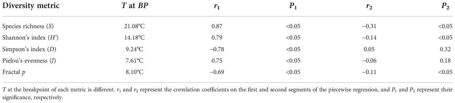
Table 1 The temperature (T) at the breakpoint (BP) of diversity and the correlation between T and diversity.

Results

SST ranges from −0.28 ± 0.01 to 29.60 ± 0.05°C. SST at the breakpoint of S, H’, D, and J are 21.08, 14.18, 9.24 and 7.61°C, respectively (Table 1). In the first segment of the piecewise regression (Figure 1), S, H’, and J are positively correlated with T (r_S1 = 0.87, r_H’1 = 0.79, r_J1 = 0.75). D is negatively correlated with T (r_D1 = −0.78). Four metrics are significantly correlated with SST (P< 0.05). In the second segment of the piecewise regression (Figure 1), S and H’ decrease significantly as SST increases (r_S2 = -0.31, r_H'2= -0.14, P< 0.05). D and J are not significantly correlated with T (P > 0.05) (Table 1). As T increases, D increases and J decreases (r_D2 = 0.05, r_J2 = −0.06).

FIGURE 1

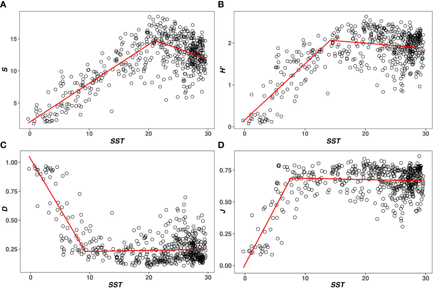
Figure 1 The T–diversity relationships are measured by (A) Species Richness (S), (B) Shannon’s index (H’), (C) Simpson’s index (D), and (D) Pielou’s evenness (J). The red line represents the result of piecewise regression, noting that S, H’, D, and J all show a unimodal relationship with T.

The R² of the fractal model to the BFD data is from 0.632 to 1.000, and more than 86% is above 0.8 (see Supplementary Table 2). SST at the breakpoint of p is 8.10°C. When SST< 8.10°C, p decreases pronouncedly as SST increases (r_p1 = −0.69, P< 0.05). When SST > 8.10°C, p decreases slightly with SST (r_p2 = −0.11, P< 0.05) and tends to be flat (Figure 2). The SST–p relationships are significantly negative over the entire SST range (see the non-line regression in Figure 2, P< 0.05).

FIGURE 2

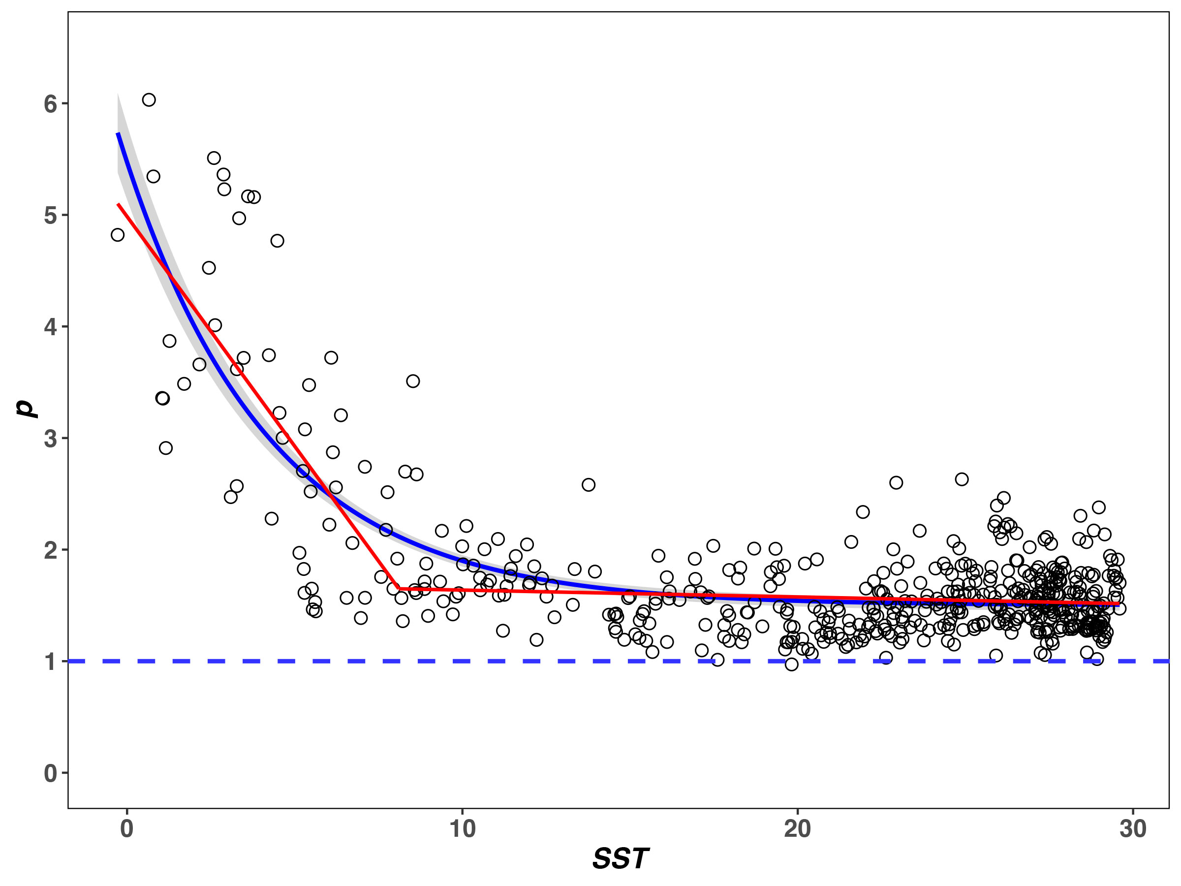
Figure 2 Relationships between SST (T) and fractal p for the BFD data. The red line represents the result of piecewise regression, noting that p changes in the same direction as T increases (r_p1 = −0.69, r_p2 = −0.11). Non-line regression results are significant (blue line with gray 99% confidence limits, results: y = −3.970e^-0.23x + 1.501, R² = 0.631, P< 0.05).

Although the bootstrap simulation is used, the results are found to be mostly consistent (see Supplementary Table 1). Thus, only the relationships between T and each metric without the bootstrap simulation are presented (Table 1 and Figures 1, 2).

Discussion

The correlation between temperature (T) and species diversity has fascinated and occupied scientists for centuries (von Humboldt, 1871; Pianka, 1966; Brown, 2014). Ecologists generally suggested that increasing T promoted higher rates of speciation or provided more tolerable living conditions leading to greater diversity (Allen et al., 2002; Currie et al., 2004; Tittensor et al., 2010). However, climatologists often implied that climate warming would have negative biological consequences triggering a decline in diversity (Cheung et al., 2009; Mora et al., 2013). Thus, how diversity relates to T has remained controversial (Yasuhara and Danovaro, 2016). Since coastal T may change rapidly in the coming decades (Zhu et al., 2021), a better understanding of the T–diversity relationship is one of the central problems in current research (Cheung et al., 2009; Brown, 2014; Yasuhara et al., 2020).

Yasuhara stated that “when considered over a sufficiently broad T range, the T–diversity relationship appears to be unimodal” (Yasuhara and Danovaro, 2016). This idea stems from a unimodal model, noting that fewer species can physiologically tolerate conditions in extremely cold or warm places than in other sites. Thus, S will show a peak at intermediate T (Currie et al., 2004). The well-known unimodal depth–diversity relationship was considered to support the unimodal model (Yasuhara and Danovaro, 2016; Yasuhara et al., 2020).

In this study, S, H’, and J show similar unimodal relationships with T (Figures 1A, B, D). Their relationships are positive below T at the breakpoint (r_S1 = 0.87, r_H’1 = 0.79, r_J1 = 0.75) and negative over T at the breakpoint (r_S2 = −0.31, r_H’2 = −0.14, r_J2 = −0.06). The T–D relationship is opposite to that of the other three metrics in two segments of the piecewise regression (r_D1 = −0.78, r_D2 = 0.05). However, D represents the species dominance in a community. The lower the D, the higher the diversity (Pielou, 1975). Thus, four metrics are not completely positive or negative with T. Species diversity measured by four metrics increases first and then decreases with increasing T. This is basically consistent with the expectation of the unimodal model (Yasuhara and Danovaro, 2016).

As noted before, the unimodal model is mostly derived based on the relationship between T and S (Yasuhara and Danovaro, 2016). However, S only represents one aspect of species diversity. It has a number of other components, such as dominance (D) and evenness (J) (Hill, 1973; Pielou, 1975; Willig and Presley, 2013). A better understanding of the T–diversity relationship needs to take these components into account (Pielou, 1975; Stevens and Willig, 2002; Willig and Presley, 2013). According to the piecewise regression results (Table 1), T at the breakpoints of D and J are apparently lower than that of S. This means that dominance has started to increase and evenness has started to decrease, when S is still increasing with T. Although the present results based on a single database may not be very universal, they at least imply that S cannot describe some changes that have occurred in species diversity. Therefore, this study suggests that evenness and dominance should be considered when investigating the T–diversity relationship, as they cannot be reflected by S. Additionally, it is worth noting that the change of D and J over T at the breakpoint is less significant than that of S (P > 0.05). This means that the unimodality of dominance and evenness is not as obvious as that of S. Similar results have also been found in the study of New World bat (Stevens and Willig, 2002). Stevens and Willig characterized three aspects of diversity for bat communities and suggested that the evenness and dominance did not change significantly at the warmer lower latitudes (Stevens and Willig, 2002). Thus, whether dominance and evenness can be treated as the typical unimodal relationship also need to be further investigated.

Finally, many ecologists have suggested that the traditional diversity indices (e.g., H’, D, and J) only represent a synthetic characterization of relative abundance in a community (Pielou, 1975; Stevens and Willig, 2002; Willig and Presley, 2013), which may lead to an excessive simplification of diversity (Mouillot et al., 2000; McGill et al., 2007). Since SAD can reflect the relative abundance for each different species encountered within a community (Tokeshi, 1993; Mouillot et al., 2000; McGill et al., 2007; Ulrich et al., 2010), it is a more comprehensive description of diversity (Mouillot et al., 2000; McGill et al., 2007; Connolly et al., 2009). According to Eq. 4, p is the fractal parameter that determines SAD. The T–p relationship shows that the direction of variation of p is the same in two segments of the piecewise regression (r_p1 = −0.69, r_p2 = −0.11, P< 0.05) (Figure 2) and their relationship is significant (P< 0.05, see the non-line regression in Figure 2). This is totally different from the other metrics (S, H’, D, and J). Accordingly, it is argued here that the fractal p has an asymptotic relationship with T rather than the typical unimodal relationship.

This study assumes that p with increasing T will gradually approach the minimum 1. Firstly, when p = 1, SAD (N_r/N₁) is 1:1/2:1/3… (Eq. 4), which is consistent with Zipf’s law (Zipf, 1949). Secondly, in previous studies, Su suggested that Zipf’s law (1:1/2:1/3…) might be a general pattern of SAD (Su, 2018), which is supported by nearly 20,000 community samples. Thirdly, Su (2018) proposed two hypotheses to elucidate this pattern. H₁: Species diversity was determined by the entropy that increased with the energy transformation. H₂: The total assimilated energy of the community (E_T) was finite. These two hypotheses provide a direction for the interpretation of the T–p relationship.

(1) N_T/N₁ (Eq. 6) is an effective number of species diversity, which is related to Rényi’s entropy (Rényi, 1961; Hill, 1973). According to H₁, increasing entropy with T leads to the rise of N_T/N₁ (Sethna, 2006). (2) According to H₂, N_T/N₁ is finite as N_T is usually equivalent to E_T (Hutchinson, 1959; Brown, 2014). On the one hand, increasing N_T/N₁ with T will cause p to decrease (Eq. 6). On the other hand, the finiteness of N_T/N₁ determines that p ought to be higher than 1 (N_T/N₁ converges when p > 1, Eq. 6), which means that the theoretical minimum of p is 1. Therefore, if H₁ and H₂ hold true, their combined effect will make p approach the theoretical minimum 1 with increasing T. Since a lower p means a higher diversity (Su, 2016); this study conjectures that species diversity with increasing T will rise and gradually approach the theoretical maximum, which is Zipf’s law (1:1/2:1/3…).

It should be emphasized that the results of this study depend on the accuracy and representation of the dataset. In fact, although BFD has been used in many studies of diversity (Rutherford et al., 1999; Tittensor et al., 2010), there are some important biases that need to be noted here. Firstly, the “pachyderma-dutertrei intergrade” category is not recognized in BFD (King and Howard, 2003). Secondly, calcium carbonate dissolution in deep-sea sediments of the Pacific and Indian Oceans may decrease the species richness of core-top assemblages (Rutherford et al., 1999). Finally, the representation of planktonic foraminifera to other organisms (especially terrestrial taxa) is still limited (Rutherford et al., 1999; Siccha and Kucera, 2017; Yasuhara et al., 2017). Thus, more details of the T–diversity relationship in planktonic foraminifera, and their pattern in other taxa, still need to be further verified.

Conclusion

When the correlation between T and diversity was mentioned in previous studies, most of the discussions revolved around the potential impact of T on S (Allen et al., 2002; Tittensor et al., 2010; Peters et al., 2016; Yasuhara and Danovaro, 2016). However, this study indicates that (1) the T–diversity relationship is not wholly captured by S and the other aspects of diversity (especially SAD) should be considered; (2) S and H’ support the typical unimodal relationship with T, while dominance and evenness do not have significant unimodality; (3) p with increasing T may decrease and gradually approach the theoretical minimum 1 (N_r/N₁ is 1:1/2:1/3…). These points are the biggest difference between previous studies and this paper.

In the future, the relationship between T and the other aspects of diversity (e.g., evenness and dominance) should be discussed more over a broader T range. This can provide feasible guidance for dealing with the potential responses of diversity to global T changes. Additionally, the relationship between T and SAD should receive more attention and investigation. It is particularly noteworthy that the theoretical minimum of fractal p (or the theoretical maximum of diversity) can be supported by more empirical data. Finally, analyzing the T–diversity relationship from multiple aspects and exploring their underlying mechanisms are expected to enrich the theories of community ecology and biogeography.

Data availability statement

The datasets presented in this study can be found in online repositories. The names of the repository/repositories and accession number(s) can be found in the article/Supplementary Material. The code supporting the results in the paper have been archived in Figshare (https://doi.org/10.6084/m9.figshare.14933301.v10).

Ethics statement

This study does not involve related issues. Ethics approval was not required for this study.

Author contributions

QS conceived and designed this study. JG developed the mathematical models and performed statistical analyses. JG and QS wrote the manuscript. All authors contributed to the article and approved the submitted version.

Funding

This work was supported by the National Natural Science Foundation of China (Grant Nos. 42071137 and 41676113). The funders had no role in study design, data collection and analysis, decision to publish, or preparation of the manuscript.

Conflict of interest

The authors declare that the research was conducted in the absence of any commercial or financial relationships that could be construed as a potential conflict of interest.

Publisher’s note

All claims expressed in this article are solely those of the authors and do not necessarily represent those of their affiliated organizations, or those of the publisher, the editors and the reviewers. Any product that may be evaluated in this article, or claim that may be made by its manufacturer, is not guaranteed or endorsed by the publisher.

Supplementary material

The Supplementary Material for this article can be found online at: https://www.frontiersin.org/articles/10.3389/fmars.2022.1069276/full#supplementary-material

References

Allen A., Brown J., Gillooly J. (2002). Global biodiversity, biochemical kinetics, and the energetic-equivalence rule. Science 297, 1545–1548. doi: 10.1126/science.1072380

PubMed Abstract | CrossRef Full Text | Google Scholar

Brown J. H. (2014). Why are there so many species in the tropics? J. Biogeogr. 41 (1), 8–22. doi: 10.1111/jbi.12228

PubMed Abstract | CrossRef Full Text | Google Scholar

Cheung W. W., Lam V.W., Sarmiento J.L., Kearney K., Watson R., Pauly D., et al. (2009). Projecting global marine biodiversity impacts under climate change scenarios. Fish Fisheries 10 (3), 235–251. doi: 10.1111/j.1467-2979.2008.00315.x

CrossRef Full Text | Google Scholar

Connolly S. R., Dornelas M., Bellwood D. R., Hughes T. P. (2009). Testing species abundance models: A new bootstrap approach applied to indo-pacific coral reefs. Ecology 90 (11), 3138–3149. doi: 10.1890/08-1832.1

PubMed Abstract | CrossRef Full Text | Google Scholar

Currie D., Mittelbach G., Cornell H., Field R., Guégan J.-F., Hawkins B., et al. (2004). Predictions and tests of climate-based hypotheses broad-scale variation in taxonomic richness. Ecol. Lett. 7, 1121–1134. doi: 10.1111/j.1461-0248.2004.00671.x

CrossRef Full Text | Google Scholar

Danovaro R., Dell'Anno A., Pusceddu A. (2004). Biodiversity response to climate change in a warm deep sea. Ecol. Lett. 7 (9), 821–828. doi: 10.1111/j.1461-0248.2004.00634.x

CrossRef Full Text | Google Scholar

Evans K. L., Warren P.H., Gaston K.J. (2005). Species-energy relationships at the macroecological scale: A review of the mechanisms. Biol. Rev. Cambridge Philos. Soc 80 (1), 1–25. doi: 10.1017/S1464793104006517

CrossRef Full Text | Google Scholar

Gao J., Su Q. (2021). “The fractal p calculation of program for the community samples,” in Brown university's foraminiferal database.

Google Scholar

Henseler C., Nordström M. C., Törnroos A., Snickars M., Pecuchet L., Lindegren M., et al. (2019). Coastal habitats and their importance for the diversity of benthic communities: A species-and trait-based approach. Estuarine Coast. Shelf Sci. 226, 106272. doi: 10.1016/j.ecss.2019.106272

CrossRef Full Text | Google Scholar

Hill M. O. (1973). Diversity and evenness: A unifying notation and its consequences. Ecology 54 (2), 427–432. doi: 10.2307/1934352

CrossRef Full Text | Google Scholar

Hunt G., Cronin T. M., Roy K. (2005). Species–energy relationship in the deep sea: A test using the quaternary fossil record. Ecol. Lett. 8 (7), 739–747. doi: 10.1111/j.1461-0248.2005.00778.x

CrossRef Full Text | Google Scholar

Hutchinson G. (1959). Homage to santa rosalia or why are there so many kinds of animals? Am. Naturalist 93, 145–159. doi: 10.1086/282070

CrossRef Full Text | Google Scholar

King A. L., Howard W. R. (2003). Planktonic foraminiferal flux seasonality in subantarctic sediment traps: A test for paleoclimate reconstructions. Paleoceanography 18 (1), 1–17. doi: 10.1029/2002PA000839

CrossRef Full Text | Google Scholar

McGill B. J., Etienne R. S., Gray J. S., Alonso D., Anderson M.J., Benecha H.K., et al. (2007). Species abundance distributions: Moving beyond single prediction theories to integration within an ecological framework. Ecol. Lett. 10 (10), 995–1015. doi: 10.1111/j.1461-0248.2007.01094.x

PubMed Abstract | CrossRef Full Text | Google Scholar

Mora C., Wei C.-L., Rollo A., Amaro T., Baco A.R., Billett D., et al. (2013). Biotic and human vulnerability to projected changes in ocean biogeochemistry over the 21st century. PloS Biol. 11 (10), e1001682. doi: 10.1371/journal.pbio.1001682

PubMed Abstract | CrossRef Full Text | Google Scholar

Mouillot D., Leprêtre A., Andrei-Ruiz M.-C., Viale D. (2000). The fractal model: A new model to describe the species accumulation process and relative abundance distribution (rad). Oikos 90 (2), 333–342. doi: 10.1034/j.1600-0706.2000.900214.x

CrossRef Full Text | Google Scholar

Muggeo V. M. (2003). Estimating regression models with unknown break-points. Stat Med. 22 (19), 3055–3071. doi: 10.1002/sim.1545

PubMed Abstract | CrossRef Full Text | Google Scholar

Obilor E. I., Amadi E. C. (2018). Test for significance of pearson’s correlation coefficient. Int. J. Innovative Mathematics Stat Energy Policies 6 (1), 11–23. Available at: https://seahipaj.org/journals/engineering-technology-andenvironment/ijimsep/.

Google Scholar

O’Hara T. D., Tittensor D. P. (2010). Environmental drivers of ophiuroid species richness on seamounts. Mar. Ecol. 31, 26–38. doi: 10.1111/j.1439-0485.2010.00373.x

CrossRef Full Text | Google Scholar

Oksanen J., Blanchet F. G., Friendly M., Kindt R., Legendre P., McGlinn D., et al. (2020). “Vegan: Community ecology package,” in R package version 2. 5-6. 2019. Available at: https://scholar.google.com/scholar?cluster=11712188988930644900&hl=en&oi=scholarr.

Google Scholar

Peters M. K., Hemp A., Appelhans T., Behler C., Classen A., Detsch F., et al. (2016). Predictors of elevational biodiversity gradients change from single taxa to the multi-taxa community level. Nat. Commun. 7 (1), 1–11. doi: 10.1038/ncomms13736

CrossRef Full Text | Google Scholar

Pianka E. R. (1966). Latitudinal gradients in species diversity: A review of concepts. Am. Naturalist 100 (910), 33–46. doi: 10.1086/282398

CrossRef Full Text | Google Scholar

Pielou E. (1975). Ecological diversity. (New York: Wiley)

Google Scholar

Prell W., Martin A., Cullen J.L., Trend M. (1999). The brown university foraminiferal data base. IGBP PAGES/World Data Center-A Paleoclimatol. Data Contrib. Series 27, 237–249. doi: 10.1594/PANGAEA.96900

CrossRef Full Text | Google Scholar

Ray G. C. (1991). Coastal-zone biodiversity patterns. Bioscience 41 (7), 490–498. doi: 10.2307/1311807

CrossRef Full Text | Google Scholar

Rényi A. (1961). On measures of entropy and information. Proc. Fourth Berkeley Symp. Math. Statist. Prob. Univ. Calif. 1 (5073), 547–561. Available at: https://scholar.google.com/scholar?q=On+measures+of+entropy+and+information&hl=zh-CN&as_sdt=0%2C5&as_vis=1&as_ylo=1961&as_yhi=.

Google Scholar

Rutherford S., D'Hondt S., Prell W. (1999). Environmental controls on the geographic distribution of zooplankton diversity. Nature 400 (6746), 749–753. doi: 10.1038/23449

CrossRef Full Text | Google Scholar

Sethna J. (2006). Statistical mechanics: Entropy, order parameters, and complexity (UK: Oxford University Press).

Google Scholar

Siccha M., Kucera M. (2017). Forcens, a curated database of planktonic foraminifera census counts in marine surface sediment samples. Sci. Data 4 (1), 1–12. doi: 10.1038/sdata.2017.109

CrossRef Full Text | Google Scholar

Stevens R. D., Willig M. R. (2002). Geographical ecology at the community level: Perspectives on the diversity of new world bats. Ecology 83 (2), 545–560. doi: 10.1890/0012-9658(2002)083[0545:GEATCL]2.0.CO;2

CrossRef Full Text | Google Scholar

Su Q. (2016). Analyzing fractal property of species abundance distribution and diversity indexes. J. Theor. Biol. 392, 107–112. doi: 10.1016/j.jtbi.2015.12.010

PubMed Abstract | CrossRef Full Text | Google Scholar

Su Q. (2018). A general pattern of the species abundance distribution. PeerJ 6, 1–11. doi: 10.7717/peerj.5928

CrossRef Full Text | Google Scholar

Tittensor D., Mora C., Jetz W., Lotze H., Ricard D., Vanden Berghe E., et al. (2010). Global patterns and predictors of marine biodiversity across taxa. Nature 466, 1098–1101. doi: 10.1038/nature09329

PubMed Abstract | CrossRef Full Text | Google Scholar

Tokeshi M. (1993). Species abundance patterns and community structure. Adv. Ecol. Res. 24 (08), 111–186. doi: 10.1016/S0065-2504(08)60042-2

CrossRef Full Text | Google Scholar

Ulrich W., Ollik M., Ugland K. I. (2010). A meta-analysis of species–abundance distributions. Oikos 119 (7), 1149–1155. doi: 10.1111/j.1600-0706.2009.18236.x

CrossRef Full Text | Google Scholar

von Humboldt A. (1871). Ansichten der natur: Mit wissenschaftlichen erläuterungen (JG Cotta'scher Verlag).

Google Scholar

Willig M. R., Presley S. J. (2013). Latitudinal gradients of biodiversity. Levin SA. Encyclopedia Biodiversity 2, 612–626. doi: 10.1016/B978-0-12-384719-5.00086-1

CrossRef Full Text | Google Scholar

Yasuhara M., Danovaro R. (2016). Temperature impacts on deep-sea biodiversity. Biol. Rev. 91 (2), 275–287. doi: 10.1111/brv.12169

CrossRef Full Text | Google Scholar

Yasuhara M., Tittensor D. P., Hillebrand H., Worm B.. (2017). Combining marine macroecology and palaeoecology in understanding biodiversity: Microfossils as a model. Biol. Rev. 92 (1), 199–215. doi: 10.1111/brv.12223

CrossRef Full Text | Google Scholar

Yasuhara M., Wei C.-L., Kucera M., Costello M.J., Tittensor D.P., Kiessling W., et al. (2020). Past and future decline of tropical pelagic biodiversity. Proc. Natl. Acad. Sci. 117 (23), 12891–12896. doi: 10.1073/pnas.1916923117

CrossRef Full Text | Google Scholar

Zhu Z., Linong L., Xiaona Y., Zhang W., Liu W. (2021). Ar6 climate change 2021: The physical science basis. Available at: https://scholar.google.com/scholar_lookup?title=AR6%20Climate%20Change%202021&publication_year=2021&author=Z.%20Zhongming&author=L.%20Linong&author=Y.%20Xiaona&author=Z.%20Wangqiang&author=L.%20Wei.

Google Scholar

Zipf G. K. (1949). Human behavior and the principle of least effort (Cambridge: Addison Wesley Press).

Google Scholar