Field observations of seabed scour dynamics in front of a seawall during winter gales

1. Introduction

Seawalls play a key role in protecting coastal regions against erosion and recession. However, the seabed at the base of the seawall is subjected to scouring, which increases the water depth and wave height and energy in front of the structure. Larger waves lead to stronger wave loading on seawalls (Xu et al., 2022a), thereby destabilizing their structural integrity and protective capacity (Zou and Reeve, 2009; Peng et al., 2018). Failures of coastal structures are often attributed to scouring at the toe of the structure (Jayaratne et al., 2016). This highlights the importance of elucidating seawall scour processes.

The maximum scour depth has been examined to better characterize toe scouring (Xie, 1981; Fowler, 1992; Sutherland et al., 2006; Müller et al., 2007; Lee and Mizutani, 2008; Salauddin and Pearson, 2019). Scouring patterns of coastal structures have also been investigated (Tahersima et al., 2011; Tofany et al., 2014; Jayaratne et al., 2016; Pourzangbar et al., 2017c). Soft computing approaches such as artificial neural networks and genetic programming, have recently been employed to predict wave-induced scour depth at breakwaters (Pourzangbar et al., 2017a; Pourzangbar et al., 2017b; Pourzangbar et al., 2017c). Results of the models developed have been compared with empirical formulas derived from flume experiments (Xie, 1981; Sumer and Fredsøe, 2000; Lee and Mizutani, 2008). Although these studies have provided insights into seabed scouring near seawalls and breakwaters, the empirical models and numerical simulations have not yet been sufficiently validated with field measured data. Therefore, the mechanisms influencingunderlying scouring in field conditions remain unclear. Erosion processes and scouring intensity in field conditions differ substantially from the enclosed environment of experimental flumes. Longshore currents account for a considerable proportion of the total littoral drift in surf and swash zones (Austin et al., 2011; Puleo et al., 2020). However, simulation of residual currents is unachievable owing to the sidewall effect in closed-system flume tests. Disregarding longshore processes are associated with errors in prediction of sediment transport rates (Puleo et al., 2020). Further studies are needed to assess the scouring process, identify the principal influencing factor, and determine scour regularities through field investigations and observations.

To provide additional information on the dynamics of toe scouring under field conditions, a seawall situated in the Gudong area, east of the Yellow River Delta, China, was taken as the research subject. The Yellow River Delta is an important industrial zone for oil and gas exploration, salt production, and aquaculture. However, the area has undergone extensive erosion since 1976 owing to a lack of sediment supply from the Yellow River (Chu et al., 2006). Meanwhile, the Gudong seawall was constructed on the coast of the Yellow River Delta in 1985 by the Shengli Oil company to prevent seawater from invading the oil field, as well as protecting it from storm surges and wind waves. By the end of 1990, the seawall was 16.88 km long, encompassing an area of 76 km². the seabed in front of the seawall is now experiencing severe erosion, which is threatening its structural integrity.

To investigate the mechanisms underlying seabed scouring under wave action and characterize the main factors impacting sediment resuspension under hydrodynamic action, we employed a series of advanced methods, including synchrosqueezed wavelet transform (SWT) and continuous wavelet transform (CWT). Considering that strong waves in the study area primarily occur in winter, based on an in-situ observation platform, we measured waves, currents, tides, turbulence, and sediment parameters. The primary aims of the current study are to: (1) present a field example of seabed scouring in front of the Gudong seawall; (2) analyze the dynamic conditions associated with scouring; (3) discuss the primary mechanisms of sediment transport associated with seabed erosion. The findings of this study have provided additional insights into sediment dynamics in front of seawalls, thereby providing insights into a sustainable design for coastal structures that considers seafloor scouring and sea level rise.

2. Study area

Formed in 1855, the modern Yellow River Delta covers an area of > 10,000 km² (Zhang et al., 2019). Since 1855, the Yellow River has undergone 11 large-scale changes in its course (Zheng et al., 2018). By 1976, its course had changed from the Diaokou Course to the Qingshuigou Course (Figure 1A). This has resulted in severe erosion in the abandoned Diaokou lobes at the north of the delta. More recently, sediment transportation from the Yellow River to the sea has sharply decreased, while the Gudong sea area has eroded (Chu et al., 2006; Bi et al., 2014). The Yellow River Delta is rich in oil, gas, and land resources. It has the second largest oil field in China (Shengli Oil Field), as well as extensive wetland resources covering a total area of 4,167 km², including natural and artificial wetlands (Zhang et al., 2016). The Delta has a high level of species richness and diversity with 220 plant species and over 800 animal species including more than 280 bird species recorded. Moreover, it is an important habitat and site for migratory birds (Wang et al., 2014).

The Gudong seawall was constructed in the 1980s to reduce costs from oil production. Due to the area being low-lying with a large area below average sea level, the Gudong seawall is considered the most important safety barrier for the oil field (Bi et al., 2014). The Gudong coastal dam is essential for land protection and economic development (Wang et al., 2020). However, the seabed has been continuously eroded in front of the dike, forming an erosion groove parallel to the seawall near its foundations. The maximum water depth in front of the seawall reached 6–7 m by 2020, compared to a maximum depth of 2–3 m before 2000 (Xu et al., 2022a). Seabed scouring increases the water depth in front of the seawall, thereby aggravating wave conditions and increasing the wave load on sea dikes (Xu et al., 2022a). Under extreme weather conditions, the wave force may exceed the design standards for sea dikes, which may cause instability of the armor block and seawall destruction (Xu et al., 2022a).

The Yellow River mouth is a weak tidal estuary with irregular semidiurnal tides and an average tidal range of 0.73–1.77 m. Under the influence of the East Asian monsoon, wind in the Bohai Sea shows pronounced seasonal changes. In winter, the northerly wind prevails with a wind speed of 5–10 m/s, with strong winds (magnitude > 8) occurring 6.8 times each winter on average (Yang et al., 2011).In summer, the southerly wind prevails with a wind speed of 1–3 m/s.

Influenced by wind speed, waves are stronger in winter and weaker in summer. In normal conditions, the wave height is generally ~20 cm. According to Zang (1996), the maximum observed wave height is 5.2 m. Owing to the shallow water depth, the seabed is easily affected by waves, leading to suspension and transportation of sediments to the Bohai Strait and Laizhou Bay in winter and sediment deposition in summer (Wang et al., 2016).

3. Materials and methods

3.1. Bathymetric data

The historical bathymetrics of the depth profile perpendicular to the shoreline during 2000–2018 were derived from the archived dataset of the Yellow River Estuary Hydrology and Water Resources Survey Bureau. The 2020 water depth was measured using a single-beam echo-sounder on January 13–14, 2020, with tidal corrections made based on tidal elevation data from the Gudong tidal observation station (Xu et al., 2022a). The topographic map based on water depth data in 2018 is shown in Figure 1C.

3.2. Field observations on sediment dynamics

The interannual variation in the water depth profile of the survey line is shown in Figure 1D. From 2000 to 2020, the water depth at the root of the seawall increased from 2 m to 5.7 m, and the depth of the profile showed a deepening trend. To analyze scour dynamics in front of the seawall, a GD bottom observation (Figure 1B) system was deployed near the survey line (37.9363° N, 119.0576° E). Additional information on the distribution and interannual variation of water depth near the observation station, as well as the layout of bathymetric survey lines is provided in Xu et al. (2022a). The observation station was located approximately 100 m from the shore, and all the instruments were mounted on a stainless-steel platform with a height of ~0.5 m. Observations lasted from November 4 to December 4, 2021 (31 days). The stainless-steel platform was equipped with a Nortek 6 MHz Acoustic Doppler Velocimetry (ADV) to measure near-bed (0.8 m) three-dimensional flow velocity at a sampling frequency of 16 Hz. A Nortek 600 kHz acoustic wave and current (AWAC) was used to monitor surface waves and currents in the upper water column. Optical backscatter sensors (OBS, Seapoint Sensors, Inc), powered by AWAC were installed 0.4 m above the seabed. The current and OBS measurements were configured to simultaneously sample every 10 min, while wave measurements were set to sample hourly.

FIGURE 1

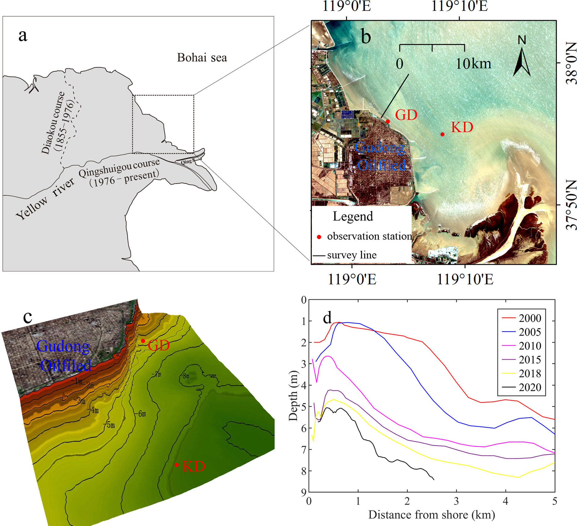
Figure 1 Overview of the study area; (A) Location of the Gudong seawall; (B) Remote sensing image of the Gudong Oilfield from lansat satellite (URI: https://landsat.gsfc.nasa.gov/); black line indicates bathymetric survey line. (C) Topographic map based on water depth data in 2018. (D) Water depth profiles of the bathymetric line in ‘b’. Red spots marked with GD and KD in (B) and (C) indicate locations of the observation stations.

From January 14 to April 19, 2020, we conducted in-situ observations at GD (37.9359° N, 119.0575° E) and KD (37.9200° N, 119.1379° E) simultaneously to compare the discrepancies of hydrodynamics in front of the seawall and the far field (Figure 1B). An AWAC were deployed at each station with the same parameter settings as the field observations from 2021, and no additional instruments were deployed.

Wind data at 10 m above the sea surface (W₁₀, unit: m/s) near the observation station were obtained from National Centers for Environmental Prediction climate forecast system version 2 (NCEP CFSv2) at 1 h intervals (URI: https://rda.ucar.edu/datasets/ds094.1/). Owing to the difficulty of collecting water samples during high winds, we collected bottom sediment near the observation station. Meanwhile, OBS sensor calibration was performed in the laboratory to establish the relationship between OBS measured turbidity values and SSC. Table 1 summarizes the instruments deployed on the stainless-steel platform.

TABLE 1

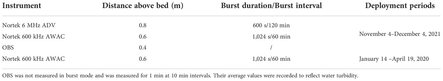
Table 1 Summary of instrumentation and sampling parameters at observation stations.

The type of bottom sediment type near the site is silty (d₅₀ = 0.068 mm, clay content CC = 2.85%) and the grain size accumulation curve for surface sediment near the observation site is shown in Figure 2.

FIGURE 2

Figure 2 Cumulative particle size distribution of soil in the bottom boundary layer of the site.

3.3. Wave parameter calculation

The accuracy of AWAC wave measurement benefits from a combination of acoustic surface tracking, velocity data, and pressure data. Acoustic surface tracking uses a vertical acoustic beam to measure water surface height. This has the advantage of reducing the impact of velocity and water depth compared to pressure sensors (Pedersen and Lohrmann, 2004). The surface wave pressure spectrum Sp(f) and directional wave spectrum were calculated using Storm software—a Nortek software for analyzing wave data measured by AWAC. Wave parameters, namely, significant wave height (Hs) and bottom wave orbital velocity (U_w) were expressed via Equations (1) and (2), respectively (Wiberg and Sherwood, 2008)

$\begin{array}{ll}Hs=4\sqrt{Sp\left(f\right)df}& (1)\end{array}$

$\begin{array}{ll}{U}_w=\sqrt{\underset{\sum }{2}i\frac{w_i^2}{sin{h}^2{k}_{i}h}{S}_{p,i}\left(f\right)\Delta f_i}& (2)\end{array}$

Where w represents the angular wave frequency, Δf is the frequency band of wave pressure spectrum, i is the number of bands, and k represents the wave number. The peak period (T_p) is defined as the period corresponding to the highest energy of Sp(f).

3.4. Wave–turbulence decomposition

Given that near-bed velocity measured by ADV is susceptible to environmental interference (Fugate and Friedrichs, 2002), strict post-processing was performed before analysis. The quality of ADV data was controlled by removing ADV-measured data points with a correlation< 70% and Signal-to-Noise ratio (SNR, unit: dB)< 5 dB. The “phase space method” was then used to detect and replace spikes in the data (Goring and Nikora, 2002).

High-frequency flow velocity measured via ADV captured changes in mean flow velocity, wave motion, and turbulence. Accurate extraction of turbulence and calculation of turbulent parameters, such as turbulent kinetic energy (TKE) and turbulence-induced sediment vertical diffusion flux (TSF) requires decomposition of these motions from the original velocity signal. Bian et al. (2018) evaluated the existing wave–turbulence decomposition methods and determined the advantages of the SWT method (Daubechies et al., 2011; Thakur et al., 2013; Bian et al., 2018). Taking the eastward velocity (u) measured via ADV as an example, it can be broken down into mean velocity $(\overline{u})$ and velocity fluctuation (u^′) . In the wave environment, (u^′) is the linear superposition of further wave orbital velocity $(u_w^{\prime })$ and turbulent fluctuation $(u_t^{\prime })$ as follows:

$\begin{array}{ll}u=\overline{u}+u^{\prime }=\overline{u}+u_t^{\prime }+u_w^{\prime }& (3)\end{array}$

Figure 3 shows the results of wave–turbulence decomposition (Burst = 28, Hs = 2.4 m). The SWT of u^′ (Figure 3A) and power spectrum analysis (Figure 3C) shows that u^′ is significantly affected by waves. At frequencies > 0.5 Hz, the power spectrum of u^′ shows a distinct inertial subrange characterized by the Kolmogorov’s “−5/3” theoretical spectrum (Bian et al., 2018; Fan et al., 2019). SWT was used to reconstruct the velocity fluctuation component at wave-dominant frequencies (Figure 3A) to obtain $u_w^{\prime }$ (Figure 3B). Meanwhile, the remainder was assigned to the turbulent component $u_t^{\prime }$ (Figure 3B). Therefore, the power spectrum of each component after wave–turbulence decomposition indicates that the components of the wave in the original velocity fluctuation were effectively removed. Meanwhile, the turbulence spectrum exhibited a pronounced “energy groove” in the wave-dominant frequencies (Figure 3C). However, the frequency range affected by the wave is relatively narrow, meaning that turbulence energy loss at the wave-dominant frequencies was negligible (Bian et al., 2018).

FIGURE 3

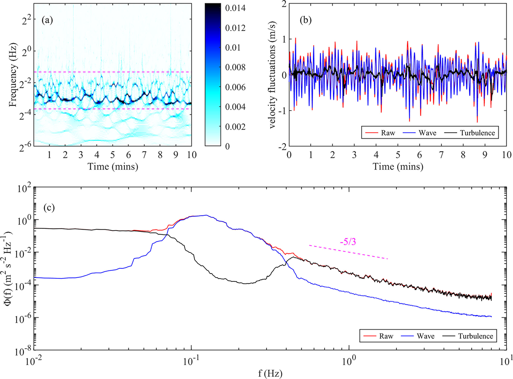
Figure 3 Wave–turbulence decomposition results of ADV-measured near bottom water motion (Burst = 28, Hs = 2.4 m). (A) Synchrosqueezed wavelet transform (SWT) of u^′ ; pink dashed lines indicate the wave-dominant frequency. (B) Time series of the original velocity fluctuation u^′ (red) and each component reconstructed using the SWT method; blue and red lines represent the wave and turbulent components, respectively. (C) Power spectra of the u^′ (red), and the decomposed wave motions (blue) and turbulence (black); pink dashed lines indicate Kolmogorov’s “−5/3” theoretical spectrum.

3.5. Bottom bed shear stress estimation

Bottom bed shear stress is a critical parameter controlling erosion, deposition, and resuspension of seabed sediments. We calculated the bottom bed shear stress induced by currents, waves, and TKE, expressed as τ_c, τ_w, and τ_TKE, respectively.

Current-induced bottom shear stress (τ_c,unit: N/m²) was calculated using the formula reported by Soulsby (1997), which relies on a specific log profile and estimates the shear stress from the first moment statistics. The bed shear stress τ_c is expressed as follows:

$\begin{array}{ll}{\tau }_c=\rho C_D{U}^2& (4)\end{array}$

$\begin{array}{ll} C_D={\left[\kappa /\ln \left(z/z_0\right)\right]}^2& (5)\end{array}$

where U (unit: m/s) is the burst-averaged velocity at height z (z = 0.8 m) collected by ADV, and z₀ = d₅₀/12 (unit: μm) indicates the roughness of the seabed (d₅₀is the median particle size, 68 μm). ρ = 1025 kg/m³ and κ = 0.4 represent the seawater density and von Karman constant, respectively.

Wave-induced bottom shear stress (τ_w, unit: N/m²) can be expressed as a function of the wave friction coefficient (f_w) and wave orbital velocity (U_w) (Grant and Madsen, 1979; Soulsby, 1997). For a wave with period T, and orbital velocity U_w, the bed shear stress τ_w is expressed as follows:

$\begin{array}{ll}{\tau }_w=\frac{1}{2}\rho f_w{U}_w^2& (6)\end{array}$

$\begin{array}{ll} f_w=1.39{\left[U_{w}T/\left(2\pi z_0\right)\right]}^{-0.52}& (7)\end{array}$

Combined shear stress of currents and waves play an important role in seabed erosion in estuaries and coastal areas (Zhu et al., 2016). Bed shear stress caused by combined wave–current action (τ_cw, unit: N/m²) is described by (Grant and Madsen, 1979) as follows:

$\begin{array}{ll}{\tau }_{cw}={\left[{\left({\tau }_w+{\tau }_c\left|\cos \phi \right|\right)}^2+{\left({\tau }_c\sin \phi \right)}^2\right]}^{1/2}& (8)\end{array}$

where φ is the angle between the current direction and wave propagation direction.

Along with currents and waves, turbulence is also critical for resuspended sediment to enter the water column. Turbulence strength determines the vertical diffusion of suspended sediment. The turbulence-induced bottom shear stress τ_TKE (unit: N/m²) is expressed as follows:

$\begin{array}{ll}{\tau }_{TKE}=C\rho TKE& (9)\end{array}$

$\begin{array}{ll}TKE=\left(\overline{u_t^{\prime 2}}+\overline{v_t^{\prime 2}}+\overline{w_t^{\prime 2}}\right)/2& (10)\end{array}$

where C is a constant (0.19) (Stapleton and Huntley, 1995; Kim et al., 2000), and TKE is calculated from the turbulence components described in Eq (3).

3.6. Spectral and wavelet analysis

Spectral and wavelet analysis are widely used in signal processing and analysis (Elsayed, 2008; Pomeroy et al., 2015). They were used in the analysis to process flow velocity and SSC data. Spectral analysis can be used to determine the frequency range of fluid motion. Wavelet analysis allows the extraction of time and frequency information to determine the intensity of each frequency component at each time of measurement. That is, the instantaneous distribution of each signal in the frequency domain (Liu and Babanin, 2004). In the present study, wavelet power spectrum was applied to turbulence-induced sediment vertical diffusion flux and momentum flux to visualize the coherent structures, which is shown in Section 5.2.

3.7. Calibration of suspended sediment concentration

Variation of SSC in the boundary layer can be obtained by combining turbidity measured using optical instruments, acoustic reflection signals from acoustic instruments, and field water samples (Yuan et al., 2008; Yuan et al., 2009; Zhao et al., 2016; Fan et al., 2019). A similar approach has been used in this study. The in-situ near-bottom water samples obtained were dried in an oven at a constant temperature of 60°C. The OBS turbidimeter, and a certain volume of distilled water, were placed in the calibration tank with a volume of 30 L, where turbidity and SSC were near 0. The dried mud samples were then gradually added to the tank and stirred for 5 min to ensure complete mixing of the suspended sediment, and the OBS recorded the turbidity simultaneously. A total of 29 sets of corresponding SSC and turbidity values were obtained. Correlation was determined using the regression method and the coefficient of determination (R²) reached 0.9928 (Figure 4). According to the calibration formula obtained, the turbidity value recorded by OBS was converted to SSC (denoted as SSC_OBS, unit: mg/L).

FIGURE 4

Figure 4 Calibration of suspended sediment concentration. (A) Linear regression of optical backscatter sensors (OBS) turbidity and suspended sediment concentration (SSC) in the laboratory. (B) Linear regression of Signal-to-Noise ratio (SNR) recorded via acoustic doppler velocimetry (ADV) and SSC_OBS. When establishing the relationship between SNR and SSC_OBS, the burst exceeding the OBS range as shown in Figure 7 was eliminated.

The SNR recorded by ADV can reflect SSC variation (Fugate and Friedrichs, 2002; Voulgaris and Meyers, 2004). We established linear regression between the logarithm of SSC_OBS and SNR value, as shown in Figure 4B. Results showed that log₁₀(SSC_OBS) was significantly correlated with SNR with an R² of 0.8689. The SNR was then transformed into high frequency SSC (denoted as c, unit: mg/L). The burst averaged value of c, was denoted as SSC_ADV (unit: mg/L).

4. Results

4.1. Waves

During the observation periods, the maximum and average values of W₁₀ were 18.0 and 7.3 m/s, respectively, with a dominant northwest wind (Figure 5A). Three weather events with relatively strong winds (W₁₀ > 10.0 m/s) occurred on November 6–11, November 21–22, and November 30–December 1, 2021 (Figure 5).

FIGURE 5

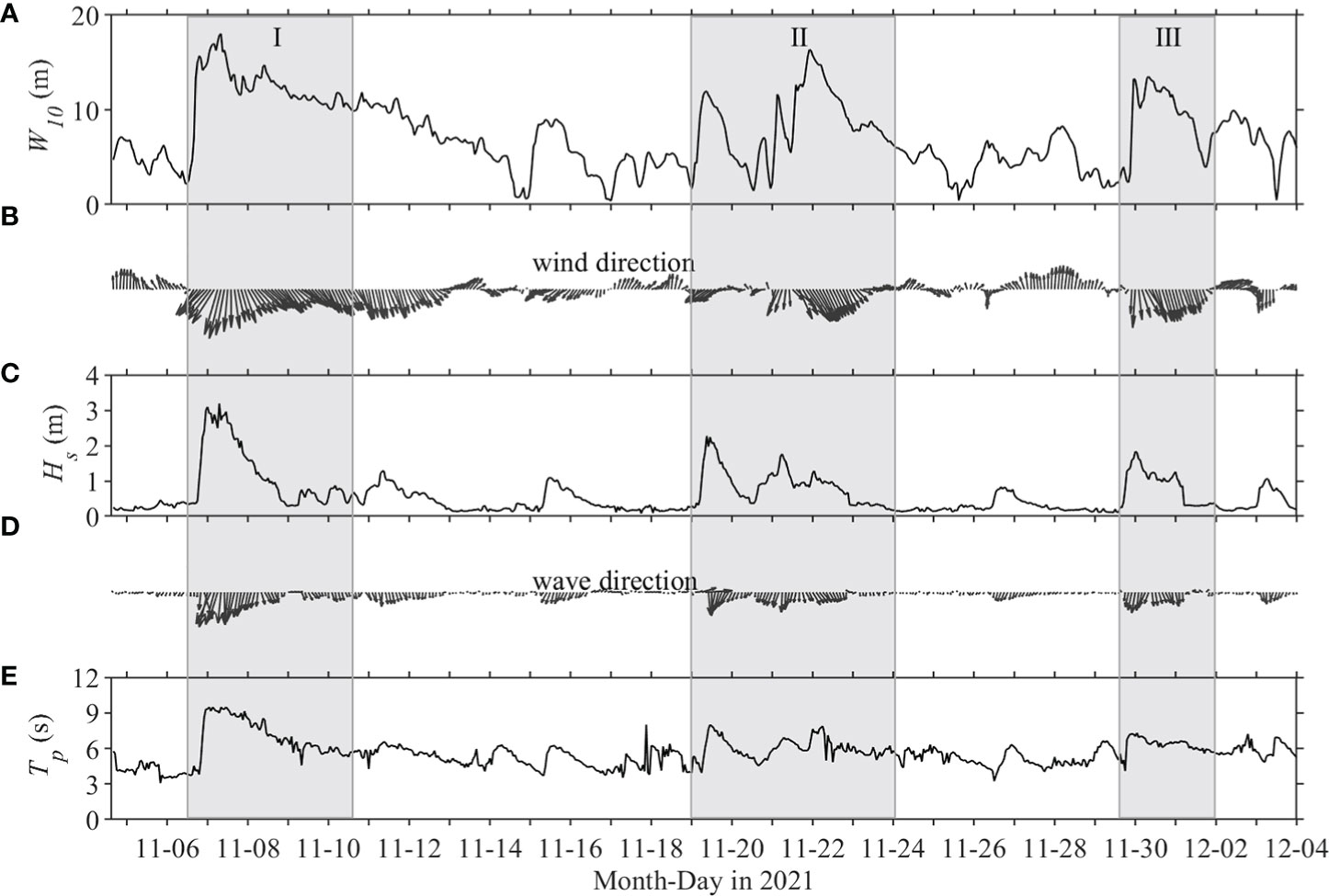
Figure 5 Time series of (A) wind speed at 10 m above ground surface (W₁₀), (B) wind direction, (C) significant wave height (Hs), (D) peak wave direction, and (E) peak wave period (Tp). Gray rectangular boxes represent weather events I, II, and III, used to discuss wave processes during observations.

At the beginning of the first strong wind weather event, the northeast wind gradually strengthened, with a W₁₀ range of 2.2–18.0 m/s. Hs rapidly increased to 3.19 m, reaching the maximum value during the observation period. From November 7 to 8, the wind direction changed to the northwest, while the W₁₀ continued to range between 10.0 and 11.0 m/s. The Hs value rapidly decreased to approximately 0.5 m, and the Tp was stable at 4–6 s. At the beginning of the second weather event, a moderate intensity northeast wind was observed (W₁₀ range: 2.4–11.9 m/s) with a rapid rise in Hs (2.27 m). On November 21, the wind direction shifted to northwest and wind speed increased to 16.4 m/s. However, the Hs was lower than that at the beginning of the second weather event. Wave growth was then limited by the transient northwest wind. In the third weather event, W₁₀ had a range of 2.4–13.5 m/s, Hs increased from 0.26 m to 1.8 m, and Tp was stable at 5–7 s. The changes in Hs and Tp maintained a relatively high level of consistency, and increased rapidly under the influence of the northeast wind and decreased slowly under the northwest wind. Under the south or northwest wind, Hs remained low, while the high wave height condition was caused by northeast winds.

4.2. Tides and currents

The time series for water level and flow velocity during the observation period are shown in Figure 6. Hs was used to reflect wave intensity and is shown in Figure 6A. The measured water level (η, unit: m) ranged from −1.3 to 1.4 m (Figure 6B). Its variation notably increased during high waves. Harmonic analysis on the time series of η using the T_tide package (Pawlowicz et al., 2002) showed that the tidal-induced water level (η_tidal, unit: m, Figure 6B) was consistent with the variation in the water level measured under normal weather conditions. During high waves, variation in the residual water level (η–η_tidal) caused by wind stress is notably greater than η_tidal (−0.5 to 0.6 m), while the maximum residual water level reaches 1.28 m. A comparison of residual water level and wind conditions shows that the rise in water level was caused by offshore winds (NE direction), while the fall in water level was associated with onshore winds (NW direction).

FIGURE 6

Figure 6 Time series of (A) significant wave height Hs, (B) variation in water level measured (blue line), tidal-induced water level from T_tide package (red line), (C) flow velocity, and (D) flow direction measured. The black dashed line represents the average orientation of the Gudong seawall. The elevation datum of the water level is defined as the average water depth (6.7 m) during the observation periods.

In calm weather conditions, the measured flow velocity (U) was< 0.3 m/s, which is nearly equivalent to the tidal current (U_tidal)value, the maximum of which was 0.28 m/s (Figure 6C). During periods of high wave activity, the flow velocity was significantly enhanced, reaching a maximum of 1.11 m/s. The enhanced velocity was primarily attributed to residual current generated by high waves. The flow direction also changed notably, indicating that strong longshore currents exceeded the reciprocating tidal currents. The average azimuth of the flow direction observed during high waves was 133°. The azimuth is the northward reference angle, and clockwise direction is denoted as positive. This is predominantly related to the orientation of the Gudong seawall located in the NW–SE direction with an average azimuth of 120° (Figure 6D).

4.3. Suspended sediment concentration and shear stress

The SSC_OBS and SSC_ADV obtained using optical and acoustic instruments after calibration was shown in Figure 7. The SSC exhibited robust coupling with Hs. In calm weather conditions, the average SSC_OBS and SSC_ADV values were approximately 300 mg/L. When wave conditions strengthened, the trends in SSC_OBS and SSC_ADV were relatively consistent, and rapidly increased to 7,137 mg/L and 12,222 mg/L, respectively. During the gale from November 7–10, the SSC_OBS value was out of range during high waves with Hs > 2.4 m, and the SSC_OBS and SSC_ADV values differed due to distinct behavior of coarse and fine particles during the decay stage of the gale. Coarse particles settled while the fine particles may have remained in suspension when Hs dropped below 0.5 m. Considering that the SSC obtained by ADV acoustic inversion is not sensitive to the dependence on particle size variation (Fugate and Friedrichs, 2002), the optical signal was more susceptible to the influence of unsettled fine particles. Therefore, SSC_OBS may be higher than SSC_ADV during the decay stage of the gale. The intra-burst standard deviation of high frequency SSC was typically< 1,000 mg/L, while a previous study reported that the quality of acoustic backscattering was superior to optical backscattering (MacVean and Lacy, 2014). Therefore, SSC_ADV was used to characterize the SSC of the bottom boundary layer.

FIGURE 7

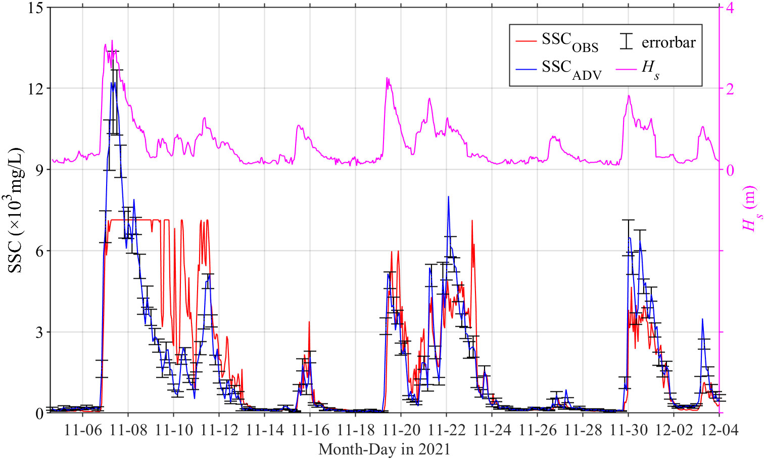
Figure 7 Time series of SSC_OBS(red line), SSC_ADV (blue line), standard deviation within burst of ADV (black error bar), and Hs (pink line).

Formation of high SSC is predominantly attributed to horizontal convective transport or the local resuspension process (Zhang et al., 2021). Horizontal convective transport is induced by the horizontal SSC gradient, while the local resuspension process is primarily induced by turbulence in the form of vertical sediment diffusion (Yuan et al., 2009). Band-pass filtering and SWT have been applied to extract the wave $(c_w^{\prime })$ and turbulent $(c_t^{\prime })$ components of high-frequency SSC fluctuation (c^′ , $c^{\prime }=c-\overline{c}$, the overbars (^—) represents the average of each burst) (Fan et al., 2019; Li et al., 2022). The power spectrum of c^′ exhibited a clear peak near the wave-dominant frequency, which was in line with velocity fluctuations. However, at frequencies > 3 Hz the power spectrum appeared to be contaminated by white noise (Figure 8). Therefore, in this study, the SWT method was applied for wave-turbulence decomposition of c^′ TSF is a more direct indicator of resuspension dynamics than SSC (Brand et al., 2010). It can be expressed as $\overline{c_t^{\prime }{w}_t^{\prime }}$, where $w_t^{\prime }$ represents the vertical velocity fluctuation extracted using the SWT method. SSC_ADV and TSF exhibited the same variation trend. High SSC_ADV is typically accompanied by high TSF values (Figure 9). This indicates that high SSC_ADV is mainly generated by local resuspension during gale events. Therefore, SSC_ADV was applied to characterize scour intensity in the study area with a focus on sediment resuspension.

FIGURE 8

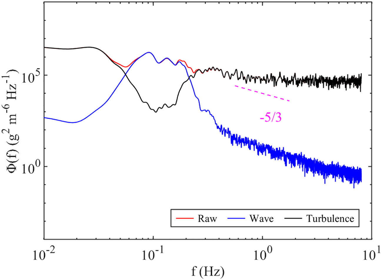
Figure 8 Power spectrum analysis of high frequency SSC fluctuations, c′(red), and the decomposed fluctuation that induced by wave ( $c_w^{\prime }$, blue) and turbulence ($c_t^{\prime }$, black).

FIGURE 9

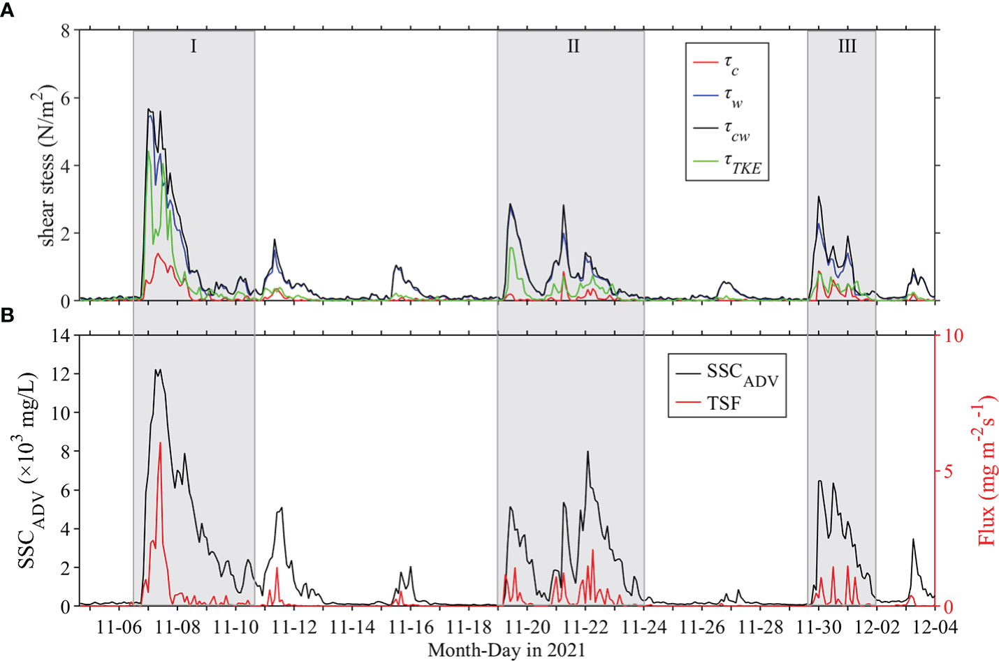
Figure 9 Time series of (A) current-induced bed shear stress (red line), wave-induced bed shear stress (blue line), combined wave-current bed shear forces (black line), turbulent-induced shear stress (green line), and (B) SSC_ADV (black line) and turbulent-induced sediment vertical diffusive flux (red line).

To analyze the principal factors controlling sediment resuspension, we calculated the bottom shear stresses generated by currents, waves, turbulence, and the combined action of waves and currents. In calm weather conditions, τ_c, τ_w, τ_cw and τ_TKE were< 0.1 N/m². Following the increase in wave energy, τ_c, τ_w, τ_cw and τ_TKE increased by 1–2 orders of magnitude reaching maximum values of 1.41 N/m², 5.48 N/m², 5.68 N/m² and 4.44 N/m² on November 7, 2021, respectively (Figure 9). The maximum τ_w value was 3.89 times that of τ_c, and τ_w dominated the change in τ_cw. Therefore, wave and current acted together in the study area, among which the effect of wave-induced bottom shear stress on the seabed exceeded that of the current.

5. Discussion

5.1. Effects of seawalls on hydrodynamics

To discuss the effects of seawalls on hydrodynamic conditions, we analyzed the waves and currents at GD and KD stations that were simultaneously observed in 2020. The time series of Hs showed similar variation patterns at the two observation sites (Figure 10A), although the statistical wave condition of KD was slightly stronger than that of GD, with the difference generally fluctuating around 0.4 m. The strong waves at KD were mainly from the NE (Figure 10B), with a mode azimuth of 32˚. However, the mode azimuth for strong waves at GD was 12˚. This was mainly due to wave refraction in front of the Gudong seawall. Furthermore, the flow velocity of GD was stronger and more sensitive to Hs than KD (Figure 10C). During periods with high waves, the flow direction at GD changed substantially with an average azimuth angle of 71° (Figure 10D). The flow direction were different from the observation results from 2021, which may have been related to the stations set up in 2020 being closer to the shore and the stronger influence of wave reflection on the hydrodynamic conditions.

FIGURE 10

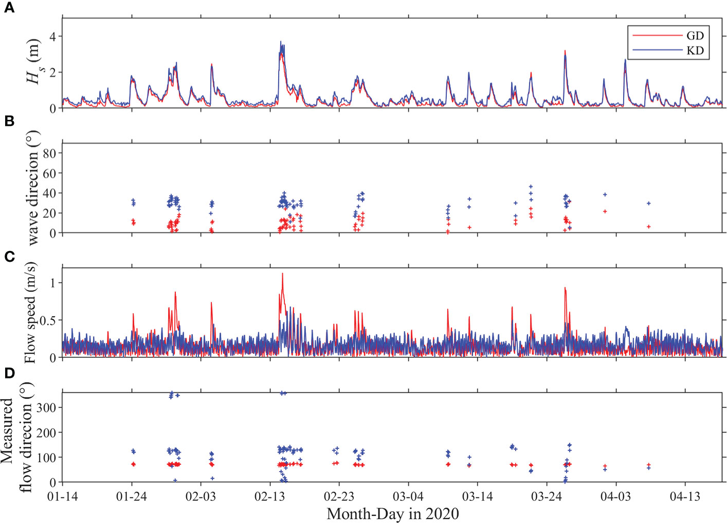
Figure 10 Time series of (A) significant wave height Hs, (B) wave direction, (C) flow speed, (D) flow direction. Red and blue represent GD and KD, respectively.

5.2. Suspending sediment transportation

To elucidate net transportation of sediment in the study area, the horizontal net flux (HNF, unit: t/m²) of sediment in the bottom boundary layer was calculated. The horizontal velocity component of the bottom boundary layer observed using ADV was projected to the coastal direction. The southeast coastal transportation was regarded as positive, while the northwest coastal transportation was negative. The horizontal net flux was then calculated, with integration of SSC_ADV and the longshore currents vector being performed in the diurnal tidal cycle.

In the small wave stages, local resuspension of sediment was relatively weak and the horizontal net flux was low (maximum< 0.3 t/m²) (Figure 11B). At this time, the net sediment transport level was in relatively dynamic balance. In contrast, during significant wave effects, most suspended sediments were transported to the southeast (Figure 11A), and the transportation flux of resuspending sediment was high, with horizontal net flux reaching a maximum of 769 t/m² per day (Figure 11B). These results highlight the significant influence of wave-induced longshore currents on transporting suspended sediment. Specifically, copious amounts of local resuspended sediments were transported southeast from the coastline of the study area by longshore currents, and local seabed erosion persisted during gales.

FIGURE 11

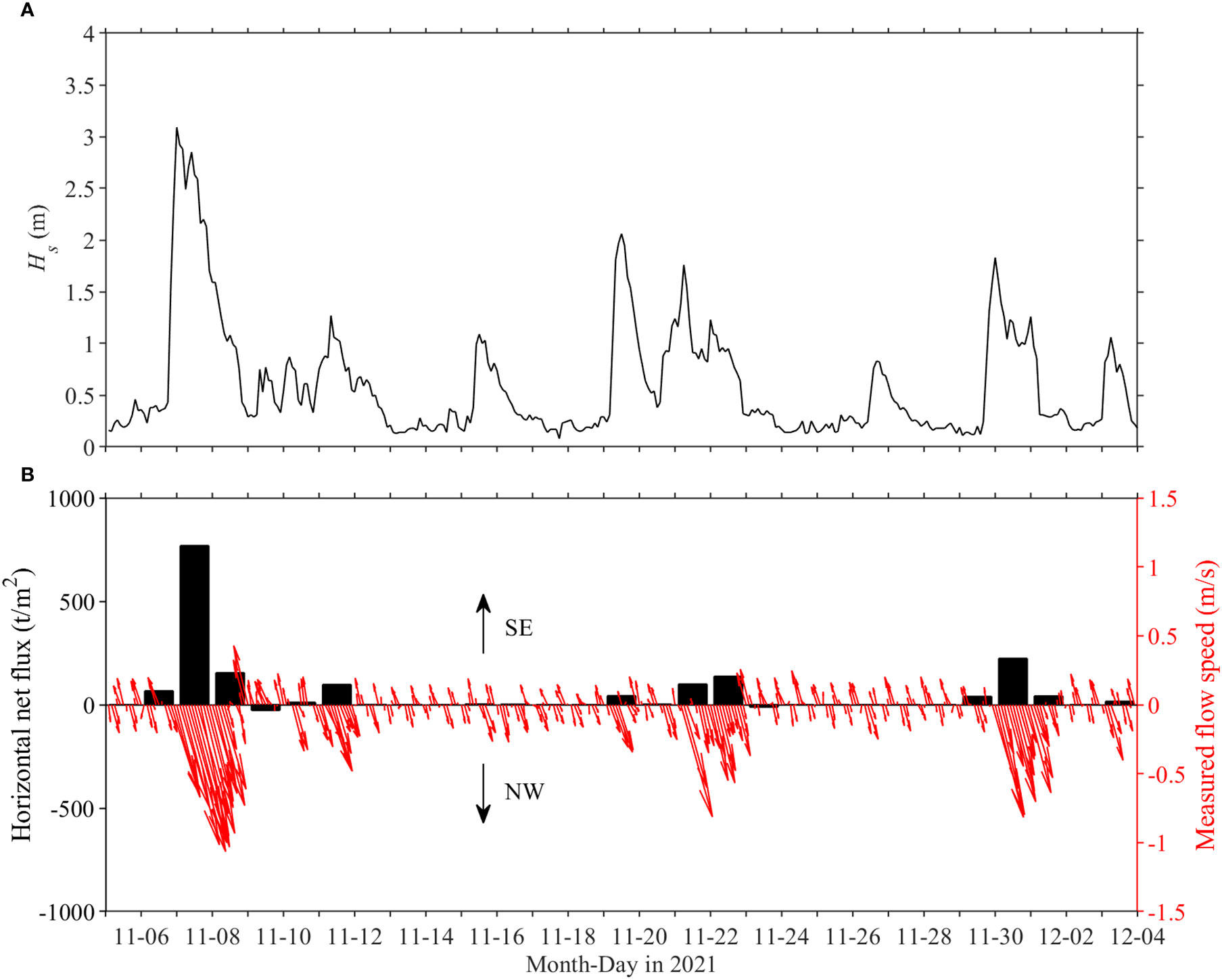
Figure 11 Time series of (A) significant wave heights Hs and (B) horizontal net fluxes of sediments in the bottom boundary layer (black bands) and horizontal velocity vectors measured via acoustic doppler velocimetry (ADV) (red arrows). Black arrows indicate the direction of sediment transport, with “SE” indicating southeast and “NW” indicating northwest.

5.3. Sediment resuspension

Sediment resuspension is a dynamic process frequently occurring in the bottom boundary layer that drives material exchange between the seabed and seawater. Sediments are mainly resuspended by waves and currents and the bottom shear stress is an key parameter to control the sediment resuspension (Zhu et al., 2016; Niu et al., 2020; Li et al., 2022). The relationship between SSC and bottom shear stress is shown in Figure 12. For all calm weather periods (Hs< 0.2 m), a linear regression was observed between SSC and τ_c, with R²< 0.1 (Figure 12A), indicating that tidal shear stress is not sufficient to resuspend the bottom sediment. For the wave-influenced episodes with Hs > 0.2 m, the R² between SSC and wave-induced bed shear stress τ_w was 0.68 (Figure 12B). During wave periods, τ_w has a larger contribution in τ_cw than in τ_c (Figure 9A, Figure 12) and SSC has a similar R² to τ_cw and τ_w. This demonstrates that wave-induced shear stress is the main contributor to total bed shear stress during large gales. This means that waves generate sufficient shear stress to resuspend sediment, which is consistent with previous studies with remote sensing (Chu et al., 2006; Zhang et al., 2018; Li et al., 2021), field investigations (Yang et al., 2011; Liu et al., 2020; Niu et al., 2020; Zhang et al., 2021), and numerical simulations (Jiang et al., 2004; Fan et al., 2020).

FIGURE 12

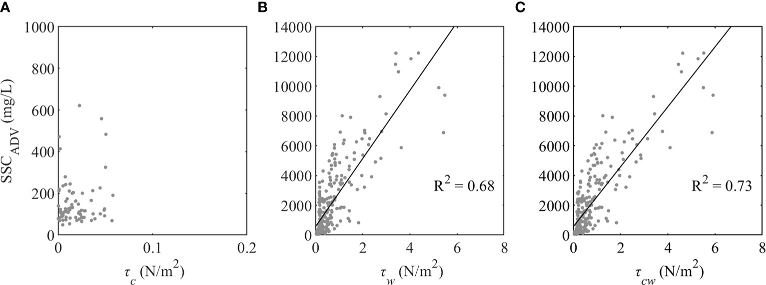
Figure 12 Scatter plots of suspended sediment concentration (SSC) and bottom shear stress of: (A) current induced when Hs< 0.2 m, (B) wave induced when Hs > 0.2 m, and (C) combination of wave and current when Hs > 0.2 m.

In the present study, τ_TKE was found to be notably enhanced during high waves. Therefore, to further characterize the effect of waves on SSC, the influence of turbulence on SSC changes was further examined. During high shear stress induced by wind and waves, SSC notably increased, with a maximum value of 12,222 mg/L. Enhanced SSC and seabed erodibility during wave periods was reflected in the response of TSF to Reynolds stress ($\overline{U_t^{\prime }{w}_t^{\prime }}$, where $U_t^{\prime }$ and $w_t^{\prime }$ represent horizontal and vertical turbulence fluctuations, respectively) (MacVean and Lacy, 2014). We regarded an Hs of 0.2 m as being the boundary between calm weather and periods with high waves and grouped all the data according to Reynolds stress values with step sizes of 0.0004 N/m². TSF and Reynolds stress generally show strong coupling, with low values in calm weather periods (Figure 13). However, TSF decreases when Reynolds stress is > 0.004 N/m². There are two likely explanations for this phenomenon. (1) Turbulence can cause vertical distribution of suspended sediments to become more uniform by enhancing the vertical diffusion, thereby decreasing the bottom sediment concentration and TSF in windy conditions. (2) Wave-induced pore pressure causes liquefaction in the seabed (Xu et al., 2022b), thereby reducing turbulence intensity. This is in line with that reported by Li et al. (2022), who indicated that SSC increased first and subsequently decreased in a typhoon event.

FIGURE 13

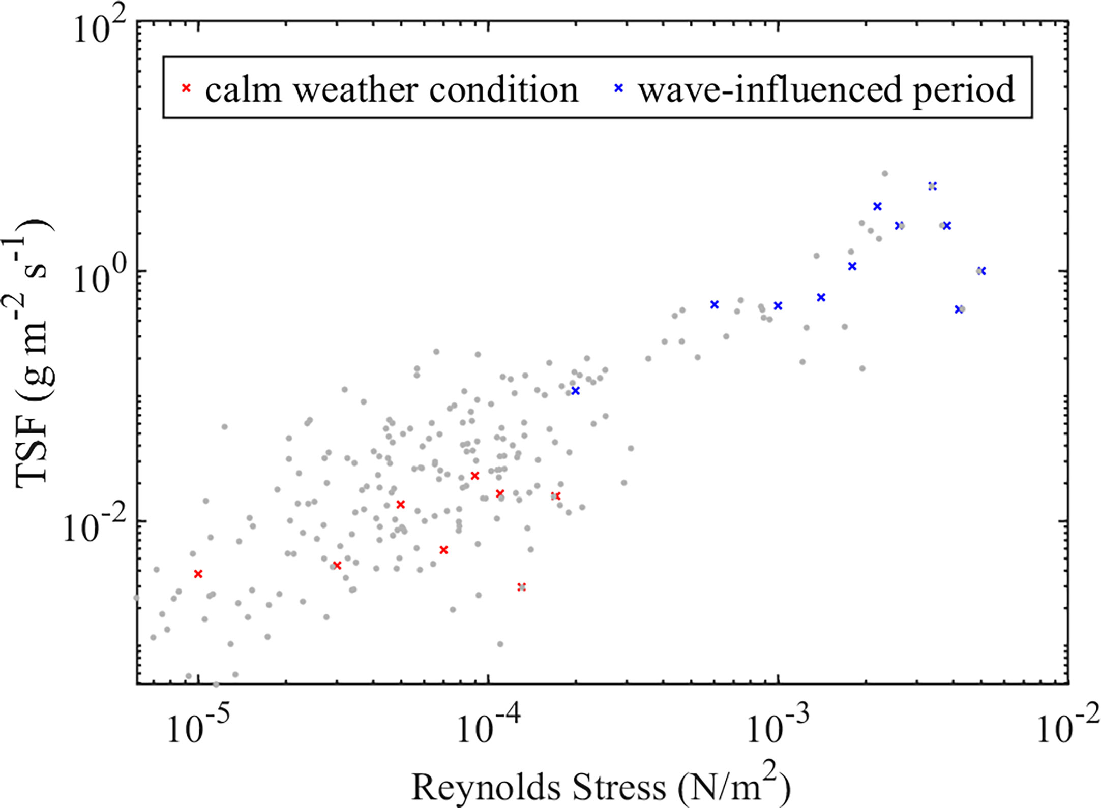
Figure 13 Scatter plot of turbulent Reynolds stress and turbulence-induced sediment vertical diffusion flux (TSF). Gray dots indicate burst-averaged values, while red and blue symbols represent calm weather conditions and wave-influenced episodes, respectively. The abscissa values of the red and blue points should be uniformly distributed; discontinuity indicates no sample points in the corresponding value range.

CWT has been used to visualize the intermittency of instantaneous Reynolds stress and TSF effectively (Torrence and Compo, 1998; Salmond, 2005; Keylock, 2007; Yuan et al., 2009; Li et al., 2022). Wavelet analysis results of instantaneous Reynolds stress and TSF signals during a gale (Burst = 28, Hs = 2.4 m) are shown in Figure 14, where the wavelet analysis passed the confidence test (95% confidence interval). The energy of Reynolds stress and TSF in the wave frequency range are relatively low. This suggests that the wave energy in the original signal was filtered out via the SWT method. Distinct plume strip structures with distribution regularity were observed between 0.2 and 8 Hz. These plume structures contained the strongest TKE, which contributed most to Reynolds stress and TSF. The high-energy bands in the Reynolds stress and TSF wavelet coefficients are consistent over time, which highlights the significant impact of turbulence on sediment resuspension.

FIGURE 14

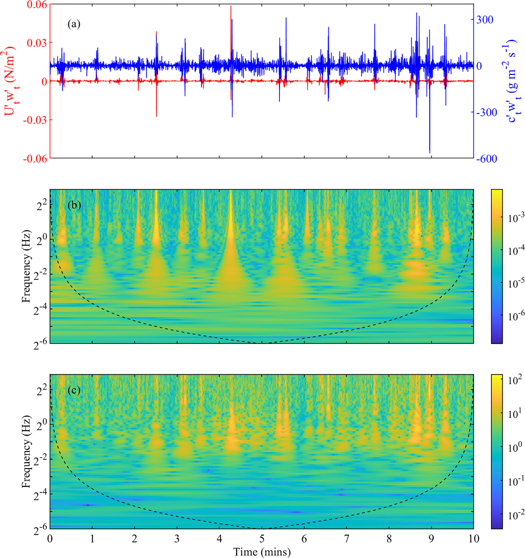
Figure 14 (A) Time series of instantaneous turbulent Reynolds shear stress ($U_t^{\prime }{w}_t^{\prime }$, red line) and instantaneous turbulent-induced sediment vertical diffusion flux ($c_t^{\prime }{w}_t^{\prime }$, blue line). Wavelet power spectra (using the Morlet wavelet) of (B) $U_t^{\prime }{w}_t^{\prime }$ and (C) $c_t^{\prime }{w}_t^{\prime }$. Black dotted line indicates the cone-of-influence caused by edge effects. The data used were obtained from burst 28, when Hs was 2.4 m.

6. Conclusions

High frequency measurements of waves, currents, tides, SSC, and turbulence were conducted for one month in the nearshore area in front of the Gudong seawall. Using advanced time–frequency analysis techniques including wavelet transform and spectrum analysis, we examined the dynamic factors associated with sediment resuspension and transport. This has provided novel insights into the formation mechanism of seabed scour and theoretical guidance for seawall protection. Our main findings are as follows:

(1) During high winds, the significant wave height was rapidly enhanced to 3.1 m, the current speed in front of the seawall increased significantly to 1.11 m/s, and the current direction changed from reciprocating flow to longshore or offshore unidirectional currents. By comparison, the maximum current speed at approximately 5 km from the seawall was 0.68 m/s, and the current direction was variable. This implies the important influence of the seawall structure on hydrodynamic conditions.

(2) In calm weather conditions, the variation of SSC was not notable and generally less than 300 mg/L. During high waves, the bottom bed shear stress and SSC increased sharply to 5.68 N/m² and 12,222 mg/L, respectively. This indicates that tidal dynamics were not sufficient for sediment resuspension. The sediment vertical diffusion flux induced by turbulence was coupled to the SSC during winter gales. This indicates that increased SSC was mainly attributed to local resuspension, and waves are the main driving force for sediment resuspension. Consistent temporal distribution of turbulence-induced sediment vertical diffusion flux and momentum flux in high wavelet power spectra highlights the important role of turbulence in sediment dynamics in front of the seawall.

(3) During high waves, the longshore currents were strengthened in front of the seawall, which intensifies sediment transportation. The daily horizontal net flux reached the maximum value (769 t/m²) during large gales, indicating the enhanced expulsion of suspended sediments from the study area, while the seabed may have been subjected to erosion.

Data availability statement

Publicly available datasets were analyzed in this study. This data can be found here: https://rda.ucar.edu/datasets/ds094.1/ and https://landsat.gsfc.nasa.gov/.

Author contributions

HS: Methodology, Investigation, Data curation, Conceptualization, Writing-original draft, Writing-review and editing. JX: Resources, Methodology, Investigation, Conceptualization, Writing-original draft, Writing-review and editing, Validation. SZ: Data curation, Investigation, Validation. GL: Resources, Data curation, Investigation. SL: Resources, Data curation, Investigation. LQ: Resources, Supervision. YY: Data curation, Writing-review. XL: Writing-review. All authors contributed to the article and approved the submitted version.

Funding

This work was supported by the National Natural Science Foundation of China [grant number 41976198, 41806072, 42276215]; the National Key Research and Development Program of China [grant number 2017YFE0133500]; the Taishan Scholar Grant to Guangxue Li.

Conflict of interest

The authors declare that the research was conducted in the absence of any commercial or financial relationships that could be construed as a potential conflict of interest.

Publisher’s note

All claims expressed in this article are solely those of the authors and do not necessarily represent those of their affiliated organizations, or those of the publisher, the editors and the reviewers. Any product that may be evaluated in this article, or claim that may be made by its manufacturer, is not guaranteed or endorsed by the publisher.

References

Austin M. J., Masselink G., Russell P. E., Turner I. L., Blenkinsopp C. E. (2011). Alongshore fluid motions in the swash zone of a sandy and gravel beach. Coast. Eng. 58 (8), 690–705. doi: 10.1016/j.coastaleng.2011.03.004

CrossRef Full Text | Google Scholar

Bian C., Liu Z., Huang Y., Zhao L., Jiang W. (2018). On estimating turbulent reynolds stress in wavy aquatic environment. J. Geophys. Res.: Oceans. 123 (4), 3060–3071. doi: 10.1002/2017JC013230

CrossRef Full Text | Google Scholar

Bi N., Wang H., Yang Z. (2014). Recent changes in the erosion–accretion patterns of the active huanghe (Yellow river) delta lobe caused by human activities. Continental. Shelf. Res. 90, 70–78. doi: 10.1016/j.csr.2014.02.014

CrossRef Full Text | Google Scholar

Brand A., Lacy J. R., Hsu K., Hoover D., Gladding S., Stacey M. T. (2010). Wind-enhanced resuspension in the shallow waters of south San Francisco bay: Mechanisms and potential implications for cohesive sediment transport. J. Geophys. Res.: Oceans. 115 (C11). doi: 10.1029/2010JC006172

CrossRef Full Text | Google Scholar

Chu Z. X., Sun X. G., Zhai S. K., Xu K. H. (2006). Changing pattern of accretion/erosion of the modern yellow river (Huanghe) subaerial delta, China: Based on remote sensing images. Mar. Geol. 227 (1), 13–30. doi: 10.1016/j.margeo.2005.11.013

CrossRef Full Text | Google Scholar

Daubechies I., Lu J., Wu H.-T. (2011). Synchrosqueezed wavelet transforms: An empirical mode decomposition-like tool. Appl. Comput. Harmonic. Anal. 30 (2), 243–261. doi: 10.1016/j.acha.2010.08.002

CrossRef Full Text | Google Scholar

Elsayed M. A. K. (2008). Application of continuous wavelet analysis in distinguishing breaking and nonbreaking waves in the wind-wave time series. J. Coast. Res. 241, 273–277. doi: 10.2112/05-0443.1

CrossRef Full Text | Google Scholar

Fan Y., Chen S., Pan S., Dou S. (2020). Storm-induced hydrodynamic changes and seabed erosion in the littoral area of yellow river delta: A model-guided mechanism study. Continental. Shelf. Res. 205, 104171. doi: 10.1016/j.csr.2020.104171

CrossRef Full Text | Google Scholar

Fan R., Wei H., Zhao L., Zhao W., Jiang C., Nie H. (2019). Identify the impacts of waves and tides to coastal suspended sediment concentration based on high-frequency acoustic observations. Mar. Geol. 408, 154–164. doi: 10.1016/j.margeo.2018.12.005

CrossRef Full Text | Google Scholar

Fowler J. E. (1992). “Scour problems and methods for prediction of maximum scour at vertical seawalls,” in Technical report CERC-92-16. Ed. W E. S. (Vicksburg, MS, USA: Us Army Corps of Engineers. Coastal Engineering Research Center).

Google Scholar

Fugate D. C., Friedrichs C. T. (2002). Determining concentration and fall velocity of estuarine particle populations using ADV, OBS and LISST. Continental. Shelf. Res. 22 (11), 1867–1886. doi: 10.1016/S0278-4343(02)00043-2

CrossRef Full Text | Google Scholar

Goring D. G., Nikora V. I. (2002). Despiking acoustic Doppler velocimeter data. J. Hydraulic. Eng. 128 (1), 117–126. doi: 10.1061/(ASCE)0733-9429(2002)128:1(117

CrossRef Full Text | Google Scholar

Grant W. D., Madsen O. S. (1979). Combined wave and current interaction with a rough bottom. J. Geophys. Res.: Oceans. 84 (C4), 1797–1808. doi: 10.1029/JC084iC04p01797

CrossRef Full Text | Google Scholar

Jayaratne M. P. R., Premaratne B., Adewale A., Mikami T., Matsuba S., Shibayama T., et al. (2016). Failure mechanisms and local scour at coastal structures induced by tsunami. Coast. Eng. J. 58 (4), 1640017–1640011-1640017-1640038. doi: 10.1142/S0578563416400179

CrossRef Full Text | Google Scholar

Jiang W., Pohlmann T., Sun J., Starke A. (2004). SPM transport in the bohai Sea: field experiments and numerical modelling. J. Mar. Syst. 44 (3), 175–188. doi: 10.1016/j.jmarsys.2003.09.009

CrossRef Full Text | Google Scholar

Keylock C. J. (2007). The visualization of turbulence data using a wavelet-based method. Earth Surface. Processes. Landforms. 32 (4), 637–647. doi: 10.1002/esp.1423

CrossRef Full Text | Google Scholar

Kim S. C., Friedrichs C. T., Maa J. P. Y., Wright L. D. (2000). Estimating bottom stress in tidal boundary layer from acoustic Doppler velocimeter data. J. Hydraulic. Eng. 126 (6), 399–406. doi: 10.1061/(ASCE)0733-9429(2000)126:6(399

CrossRef Full Text | Google Scholar

Lee K.-H., Mizutani N. (2008). Experimental study on scour occurring at a vertical impermeable submerged breakwater. Appl. Ocean. Res. 30 (2), 92–99. doi: 10.1016/j.apor.2008.06.003

CrossRef Full Text | Google Scholar

Li P., Chen S., Ji H., Ke Y., Fu Y. (2021). Combining landsat-8 and sentinel-2 to investigate seasonal changes of suspended particulate matter off the abandoned distributary mouths of yellow river delta. Mar. Geol. 441, 106622. doi: 10.1016/j.margeo.2021.106622

CrossRef Full Text | Google Scholar

Li L., Ren Y., Wang X. H., Xia Y. (2022). Sediment dynamics on a tidal flat in macro-tidal hangzhou bay during typhoon mitag. Continental. Shelf. Res. 237, 104684. doi: 10.1016/j.csr.2022.104684

CrossRef Full Text | Google Scholar

Liu P. C., Babanin A. V. (2004). Using wavelet spectrum analysis to resolve breaking events in the wind wave time series. Annales. Geophys. 22, 3335–3345. doi: 10.5194/angeo-22-3335-2004

CrossRef Full Text | Google Scholar

Liu X., Zhang H., Zheng J., Guo L., Jia Y., Bian C., et al. (2020). Critical role of wave–seabed interactions in the extensive erosion of yellow river estuarine sediments. Mar. Geol. 426, 106208. doi: 10.1016/j.margeo.2020.106208

CrossRef Full Text | Google Scholar

MacVean L. J., Lacy J. R. (2014). Interactions between waves, sediment, and turbulence on a shallow estuarine mudflat. J. Geophys. Res.: Oceans. 119 (3), 1534–1553. doi: 10.1002/2013JC009477

CrossRef Full Text | Google Scholar

Müller G., Allsop W., Bruce T., Kortenhaus A., Pearce A., Sutherland J., et al. (2007). The occurrence and effects of wave impacts. Proc. Inst. Civil. Eng. - Maritime. Eng. 160 (4), 167–173. doi: 10.1680/maen.2007.160.4.167

CrossRef Full Text | Google Scholar

Niu J., Xu J., Li G., Dong P., Shi J., Qiao L. (2020). Swell-dominated sediment re-suspension in a silty coastal seabed. Estuarine. Coast. Shelf. Sci. 242, 106845. doi: 10.1016/j.ecss.2020.106845

CrossRef Full Text | Google Scholar

Pawlowicz R., Beardsley B., Lentz S. (2002). Classical tidal harmonic analysis including error estimates in MATLAB using T_TIDE. Comput. Geosci. 28 (8), 929–937. doi: 10.1016/S0098-3004(02)00013-4

CrossRef Full Text | Google Scholar

Pedersen T., Lohrmann A. (2004). “(2004, 9-12 nov. 2004). possibilities and limitations of acoustic surface tracking,” in Oceans '04 MTS/IEEE Techno-Ocean '04 (IEEE Cat. No.04CH37600). Kobe, Japan: MTT/IEEE, 3, 1428–1434.

Google Scholar

Peng Z., Zou Q.-P., Lin P. (2018). A partial cell technique for modeling the morphological change and scour. Coast. Eng. 131, 88–105. doi: 10.1016/j.coastaleng.2017.09.006

CrossRef Full Text | Google Scholar

Pomeroy A. W. M., Lowe R. J., Dongeren A. R. V., Ghisalberti M., Bodde W., Roelvink D. (2015). Spectral wave-driven sediment transport across a fringing reef. Coastal. Eng. 98, 78–94. doi: 10.1016/j.coastaleng.2015.01.005

CrossRef Full Text | Google Scholar

Pourzangbar A., Brocchini M., Saber A., Mahjoobi J., Mirzaaghasi M., Barzegar M. (2017a). Prediction of scour depth at breakwaters due to non-breaking waves using machine learning approaches. Appl. Ocean. Res. 63, 120–128. doi: 10.1016/j.apor.2017.01.012

CrossRef Full Text | Google Scholar

Pourzangbar A., Losada M. A., Saber A., Ahari L. R., Larroudé P., Vaezi M., et al. (2017b). Prediction of non-breaking wave induced scour depth at the trunk section of breakwaters using genetic programming and artificial neural networks. Coast. Eng. 121, 107–118. doi: 10.1016/j.coastaleng.2016.12.008

CrossRef Full Text | Google Scholar

Pourzangbar A., Saber A., Yeganeh-Bakhtiary A., Ahari L. R. (2017c). Predicting scour depth at seawalls using GP and ANNs. J. Hydroinform. 19 (3), 349–363. doi: 10.2166/hydro.2017.125

CrossRef Full Text | Google Scholar

Puleo J. A., Cristaudo D., Torres-Freyermuth A., Masselink G., Shi F. (2020). The role of alongshore flows on inner surf and swash zone hydrodynamics on a dissipative beach. Continental. Shelf. Res. 201, 104134. doi: 10.1016/j.csr.2020.104134

CrossRef Full Text | Google Scholar

Salauddin M., Pearson J. M. (2019). Wave overtopping and toe scouring at a plain vertical seawall with shingle foreshore: A physical model study. Ocean. Eng. 171, 286–299. doi: 10.1016/j.oceaneng.2018.11.011

CrossRef Full Text | Google Scholar

Salmond J. A. (2005). Wavelet analysis of intermittent turbulence in a very stable nocturnal boundary layer: implications for the vertical mixing of ozone. Boundary-Layer. Meteorol. 114 (3), 463–488. doi: 10.1007/s10546-004-2422-3

CrossRef Full Text | Google Scholar

Soulsby R. L. (1997). Dynamics of marine sands: a manual for practical applications. Oceanographic. Literature. Rev. 9, 947.

Google Scholar

Stapleton K. R., Huntley D. A. (1995). Seabed stress determinations using the inertial dissipation method and the turbulent kinetic energy method. Earth Surface. Processes. Landforms. 20 (9), 807–815. doi: 10.1002/esp.3290200906

CrossRef Full Text | Google Scholar

Sumer B. M., Fredsøe J. (2000). Experimental study of 2D scour and its protection at a rubble-mound breakwater. Coast. Eng. 40 (1), 59–87. doi: 10.1016/S0378-3839(00)00006-5

CrossRef Full Text | Google Scholar

Sutherland J., Obhrai C., Whitehouse R. J. S., Pearce A. (2006). “Laboratory tests of scour at a seawall,” in Proceedings of the 3rd international conference on scour and Erosion,CURNET (Gouda, The Netherlands: Technical University of Denmark).

Google Scholar

Tahersima M., Yeganeh-Bakhtiary A., Hajivalie F. (2011). Scour pattern in front of vertical breakwater with wave overtopping. J. Coast. Res., 598–602.

Google Scholar

Thakur G., Brevdo E., Fučkar N. S., Wu H.-T. (2013). The synchrosqueezing algorithm for time-varying spectral analysis: Robustness properties and new paleoclimate applications. Signal Process. 93 (5), 1079–1094. doi: 10.1016/j.sigpro.2012.11.029

CrossRef Full Text | Google Scholar

Tofany N., Ahmad M. F., Kartono A., Mamat M., Mohd-Lokman H. (2014). Numerical modeling of the hydrodynamics of standing wave and scouring in front of impermeable breakwaters with different steepnesses. Ocean. Eng. 88, 255–270. doi: 10.1016/j.oceaneng.2014.06.008

CrossRef Full Text | Google Scholar

Torrence C., Compo G. P. (1998). A practical guide to wavelet analysis. Bull. Am. Meteorol. Soc. 79 (1), 61–78. doi: 10.1175/1520-0477(1998)079<0061:APGTWA>2.0.CO;2

CrossRef Full Text | Google Scholar

Voulgaris G., Meyers S. T. (2004). Temporal variability of hydrodynamics, sediment concentration and sediment settling velocity in a tidal creek. Continental. Shelf. Res. 24 (15), 1659–1683. doi: 10.1016/j.csr.2004.05.006

CrossRef Full Text | Google Scholar

Wang H., Gao J., Pu R., Ren L., Kong Y., Li H., et al. (2014). Natural and anthropogenic influences on a red-crowned crane habitat in the yellow river delta natural reserve 1992–2008. Environ. Monit. Assess. 186 (7), 4013–4028. doi: 10.1007/s10661-014-3676-y

PubMed Abstract | CrossRef Full Text | Google Scholar

Wang G., Li P., Li Z., Ding D., Qiao L., Xu J., et al. (2020). Coastal dam inundation assessment for the yellow river delta: Measurements, analysis and scenario. Remote Sens. 12 (21), 3658. doi: 10.3390/rs12213658

CrossRef Full Text | Google Scholar

Wang A., Wang H., Bi N., Wu X. (2016). Sediment transport and dispersal pattern from the bohai Sea to the yellow Sea. J. Coast. Res. 74 (sp1), 104–116. doi: 10.2112/SI74-010.1

CrossRef Full Text | Google Scholar

Wiberg P. L., Sherwood C. R. (2008). Calculating wave-generated bottom orbital velocities from surface-wave parameters. Comput. Geosci. 34 (10), 1243–1262. doi: 10.1016/j.cageo.2008.02.010

CrossRef Full Text | Google Scholar

Xie S. (1981). Scouring patterns in front of vertical breakwaters and their influences on the stability of the foundation of the breakwaters (Report) (Delft, Netherlands: Department of Civil Engineering, Delft University of Technology).

Google Scholar

Xu J., Sun J., Shi J., Li G., Wang X., Ding D., et al. (2022a). Increased wave load on the gudong seawall caused by seabed scour. Ocean. Eng. 250, 111005. doi: 10.1016/j.oceaneng.2022.111005

CrossRef Full Text | Google Scholar

Xu J., Dong J., Zhang S., Sun H., Li G., Niu J., et al. (2022b). Pore-water pressure response of a silty seabed to random wave action: Importance of low-frequency waves. Coast. Eng. 178, 104214. doi: 10.1016/j.coastaleng.2022.104214

CrossRef Full Text | Google Scholar

Yang Z., Ji Y., Bi N., Lei K., Wang H. (2011). Sediment transport off the huanghe (Yellow river) delta and in the adjacent bohai Sea in winter and seasonal comparison. Estuarine. Coast. Shelf. Sci. 93 (3), 173–181. doi: 10.1016/j.ecss.2010.06.005

CrossRef Full Text | Google Scholar

Yuan Y., Wei H., Zhao L., Cao Y. (2009). Implications of intermittent turbulent bursts for sediment resuspension in a coastal bottom boundary layer: A field study in the western yellow Sea, China. Mar. Geol. 263 (1), 87–96. doi: 10.1016/j.margeo.2009.03.023

CrossRef Full Text | Google Scholar

Yuan Y., Wei H., Zhao L., Jiang W. (2008). Observations of sediment resuspension and settling off the mouth of jiaozhou bay, yellow Sea. Continental. Shelf. Res. 28 (19), 2630–2643. doi: 10.1016/j.csr.2008.08.005

CrossRef Full Text | Google Scholar

Zang Q. Y. (1996). Nearshore sediment along the yellow river delta (Beijing (in Chinese: Ocean Press).

Google Scholar

Zhang X., Lu Z., Jiang S., Chi W., Zhu L., Wang H., et al. (2018). The progradation and retrogradation of two newborn huanghe (Yellow river) delta lobes and its influencing factors. Mar. Geol. 400, 38–48. doi: 10.1016/j.margeo.2018.03.006

CrossRef Full Text | Google Scholar

Zhang B., Wang R., Deng Y., Ma P., Lin H., Wang J., et al. (2019). Mapping the yellow river delta land subsidence with multitemporal SAR interferometry by exploiting both persistent and distributed scatterers. ISPRS. J. Photogramm. Remote Sens. 148, 157–173. doi: 10.1016/j.isprsjprs.2018.12.008

CrossRef Full Text | Google Scholar

Zhang S., Nielsen P., Perrochet P., Jia Y. (2021). Multiscale superposition and decomposition of field-measured suspended sediment concentrations: Implications for extending 1DV models to coastal oceans with advected fine sediments. J. Geophys. Res.: Oceans. 126 (3), e2020JC016474. doi: 10.1029/2020JC016474

CrossRef Full Text | Google Scholar

Zhang X., Zhang Y., Ji Y., Zhang Y., Yang Z. (2016). Shoreline change of the northern yellow river (Huanghe) delta after the latest deltaic course shift in 1976 and its influence factors. J. Coast. Res. 74 (10074), 48–58. doi: 10.2112/SI74-005.1

CrossRef Full Text | Google Scholar

Zhao L., Xu Y., Yuan Y. (2016). The estimation of a critical shear stress based on a bottom tripod observation in the southwest off jeju island, the East China Sea. Acta Oceanol. Sin. 35 (11), 105–112. doi: 10.1007/s13131-016-0953-3

CrossRef Full Text | Google Scholar

Zheng S., Han S., Tan G., Xia J., Wu B., Wang K., et al. (2018). Morphological adjustment of the qingshuigou channel on the yellow river delta and factors controlling its avulsion. CATENA 166, 44–55. doi: 10.1016/j.catena.2018.03.009

CrossRef Full Text | Google Scholar

Zhu Q., van Prooijen B. C., Wang Z. B., Ma Y. X., Yang S. L. (2016). Bed shear stress estimation on an open intertidal flat using in situ measurements. Estuarine. Coast. Shelf. Sci. 182, 190–201. doi: 10.1016/j.ecss.2016.08.028

CrossRef Full Text | Google Scholar

Zou Q., Reeve D. (2009). Modelling water from clouds to coast. Planet. Earth. (Autumn)., 22–23.

Google Scholar