Marine Heatwaves Offshore Central and South Chile: Understanding Forcing Mechanisms During the Years 2016-2017

Highlights

1) Detection of MHWs from 1982 to 2020 with satellite data.

2) 5-months long MHW offshore Patagonia.

3) Combination of reduced winds and advected warm water that favoured MHW development.

Additional content available at: https://dox.uliege.be/index.php/s/i3JQbteimolWYkr.

It contains the different metrics associated with all MHWs detected in the 3 studied areas (Northern, Transition and Southern areas): event number; duration; start, end and peak date of each event; mean, maximal and cumulative intensity; variation of the intensity; onset and decline rate.

1 Introduction

Extreme warming events in the oceans have become more frequent over the years (Oliver et al., 2018), partly due to human induced global warming (Laufkötter et al., 2020). Lima and Wethey (2012) estimated that between the 1980s and the 2010s, 38% of the world’s coastal zones suffered from an increase of extremely warm SST events. More recently, the IPCC has estimated in 2021 that the frequency of marine heatwaves (MHWs) has doubled since the 1980s and is believed to continue to increase, particularly in the coastal zones (IPCC, 2021). Considered as anomalously warm events, MHWs are described by their duration, intensity, rate of evolution and spatial extent. Their severity depends on both absolute SST and on local seasonal SST variability, meaning that a high temperature above the threshold does not always imply a severe MHW. Diverse factors, both atmospheric (e.g. reduced winds, higher air temperatures) and oceanographic (e.g. advection of warm waters, weaker than usual upwellings) ones with different time and spatial scales can lead to ocean’s mixed layer warming, inducing formation, maintenance and disappearance of MHWs (e.g. Holbrook et al., 2019). However, although the mechanisms that contribute to the formation of such events are becoming well known, the way they interplay to initiate and maintain MHWs remains uncertain.

The consequences of such extreme events, which can extend up to 100 m depth (e.g. Pearce and Feng, 2013; Jackson et al., 2018; Su et al., 2021), are diverse, ranging from ecosystems damages such as mass mortality, species migrations, ecosystem’s communities shifts (e.g. Smale et al., 2019), to reduced fisheries and aquaculture production (e.g. Oliver et al., 2017; Cheung and Frölicher, 2020), to modifications of the ocean’s properties (e.g. altering carbon cycle and water column stratification, reducing dissolved oxygen concentration or preventing sea ice formation; Brauko et al., 2020; Hu et al., 2020; Carvalho et al., 2021; Mignot et al., 2021).

The Chilean Patagonia, extending from 41.5°S to 56°S and bordered by the Southeast Pacific Ocean, is characterised by a complex fragmented coast forming one of the largest fjord regions in the world (Pantoja et al., 2011). Freshwater inputs through the fjords and the relatively cold and stable coastal oceanic conditions confers to Patagonia an ideal environment for aquaculture farming (Iriarte, 2018; FAO, 2019), thus being a region with a major importance in the country’s economy. Due to its sensitive environment and its economic importance, this region is particularly vulnerable to global warming (Yáñez et al., 2017; Castilla et al., 2021; Soto et al., 2021). Patagonia has already experienced the global change consequences in the form of melting glaciers (e.g. Porter and Santana, 2014), reduced precipitations (Boisier et al., 2016; León-Muñoz et al., 2018; Aguayo et al., 2021) associated with more frequent droughts (Garreaud, 2018a; Winckler-Grez et al., 2020), reduced river discharge modifying nutrient supply, turbidity and salinity (e.g. Soto et al., 2019; Winckler-Grez et al., 2020) and harmful algal blooms (HABs; León-Muñoz et al., 2018). More precisely, during the first half of 2016, Patagonia experienced very uncommon conditions with warmer temperatures, a severe drought which had reduced the streamflow by -30% to -60%, and experienced a very strong HAB development (Garreaud, 2018a) in a global context of drought in subtropical Southeast Pacific Ocean since 2010 partly due to large-scale climate forcings (Garreaud et al., 2020). However, to the best of our knowledge, MHWs have not been studied yet in this region, despite the ecosystem’s vulnerability. The first objective of this study is to realise a global assessment of the MHWs that have occurred off Central and South Chile over the last 4 decades (1982 to 2020). The second objective is to analyse the metrics of those MHWs (frequency of the events, duration and average and maximal intensity) in order to determine when the most important events occurred and if long-term trends can be observed. In addition, decadal trends of the MHWs’ metrics and of the SST will also be assessed. The third objective of this study is to have a better understanding of the factors that contribute to the formation of exceptional MHW conditions that have occurred during the 2016-2017 period, as the MHWs observed at that time were particularly intense and long.

This paper is organised as follows: in section 2, we describe the data used for the MHWs detection and for the understanding of the atmospheric and oceanic context while the MHWs were occurring. An overview of the MHWs that have occurred between 1982 and 2020 is presented in section 3, as well as a focus on the MHW conditions and their forcings over the period 2016-2017. Then, the MHWs detected in 2016-2017 are placed in a larger context and the possible consequences of the MHWs on fjord ecosystems are exposed in section 4. Section 5 provides a summary of the main results of the study.

2 Material And Methods

2.1 Study Area

Chile, bordered to the West by the South Pacific Ocean and to the East by the Andean Cordillera, extends over more than 4300 km from 17°S to 56°S (Figure 1). The Cordillera has a major role in Chilean hydrology as it regulates the climate by controlling precipitations due to the orographic effect (Viale and Garreaud, 2015; Aceituno et al., 2021). The climate and oceanic circulation off the southern part of Chile, the Patagonia (characterised by fjord ecosystems), are forced by large scale atmospheric systems. The two main ones are the Westerly Winds belt at midlatitudes and the basin-scale South Pacific Subtropical Anticyclone extending over the Southeast Pacific. The seasonal North-South migration of the two atmospheric systems is largely influencing the oceanic circulation by inducing the north-south migration of the South Pacific Current (Pérez- Santos et al., 2019; Strub et al., 2019). Thus, the wind-induced currents are also alternating from North to South direction with respectively equatorward currents in summer and poleward currents in winter along central coasts of Chile (Thiel et al., 2007; Strub et al., 2019). Consequently, along the coasts, currents are mostly equatorward north of 37°S (Sobarzo et al., 2007), North-South alternating between 37°S and 46°S, and mostly poleward south of 46°S (Strub et al., 2019). Our study region will therefore be separated in 3 areas according to the main currents circulation: as highlighted by Strub et al. (2019), the region between 38°S to 46°S represents a “transition zone” where the currents are alternating from North to South. This zone, representing North Patagonia, will constitute our central study area, referred to as the “Transition area” in the study. The two other studied areas are North and South of the Transition one, the first one extending from 29°S to 38°S and corresponding to Central Chile, named in this study the “Northern area”, and the second one being the South Patagonia, 46°S to 55°S, named in this study “Southern area”. Longitudinally, the areas were delimited in order to have a similar oceanic surface: Northern area is limited from -82°E to -71°E; Transition area from -86°E to -72°E; Southern area from -89°E to -74°E.

FIGURE 1

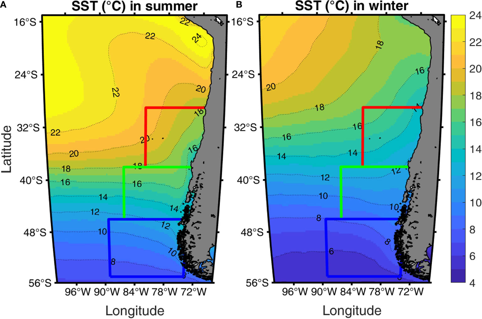
Figure 1 Mean sea surface temperature (SST; °C) in Southeast Pacific during summer (A) and winter (B). Seasonal averaged SST has been calculated over 1982-2020. Studied areas are indicated by the coloured squares: in red the Northern area (-82°E to -71°E and 38°S to 29°S); in green the Transition area (-86°E to -72°E and 46°S to 38°S); in blue the Southern area (-89°E to -74°E and 55°S to 46°S).

2.2 Data

The SST was needed to first calculate the SST climatology and secondly to calculate the SST anomaly. The SST climatology was calculated using the reanalysed product Optimum Interpolated Sea Surface Temperature (OISSTv2) provided by NOAA (available at https://psl.noaa.gov/data/gridded/data.noaa.oisst.v2.highres.html) which has a daily resolution. OISSTv2 is one of the longest temporal global SST data available and makes available 39 years of daily data with a spatial resolution of 1/4 degree, from 1982 to 2020. This dataset was used for MHW detection as advised by Hobday et al. (2016) and also to calculate SST long-term trends (described in section 2.4). To calculate the SST anomaly, we choose to use another dataset. Indeed, reanalysed products tend to be overly smooth (e.g. Subrahmanyam, 2015); we therefore preferred to create ourselves an L4 dataset instead of relying on existing ones to retain as much as possible SST variability. We decided to use the SST satellite dataset provided by the Advanced Microwave Scanning Radiometer 2 instrument (AMSR-2) onboard Global Change Observation Mission satellite, having a 1/4 degree resolution and being available at http://www.remss.com. Although our study focuses on the 2016-2017 MHWs, we downloaded the satellite data over the whole available period (2012-07-03 to 2020-12-31) for the whole Pacific Ocean. While microwaves do not interfere with clouds, they do interfere with rain; thus satellite data are still incomplete (36% of missing data on average). Reconstruction of the satellite SST field was performed with DINEOF as described in section 2.3. SST anomalies were calculated by doing the difference between the reconstructed SST data and the daily climatology.

Sea level pressure and air temperature 2 meters above surface were downloaded from 1982 to 2020 using the European Centre for Medium-Range Weather Forecast (ECMWF) reanalysis data (ERA5) available at https://cds.climate.copernicus.eu/#!/home. They both have a spatial resolution of 1/4 degree and a daily temporal resolution. Daily and monthly average atmospheric temperature anomalies were calculated using the data described above doing respectively the difference between daily and monthly air temperature and long-term daily and monthly mean from 1982 to 2020. Same for daily and monthly sea level pressure anomalies.

Zonal and meridional winds components 10 meters above surface, also downloaded from the ECMWF, were analysed over the period 2012 to 2020 (hourly temporal resolution and a spatial resolution of 1/4 degree) and wind speed was calculated from u and v component (respectively eastward and northward components).

Time series of atmospheric temperature, sea level pressure, winds and anomalies for both atmospheric pressure and temperature were also calculated and a 3-months Gaussian filter was applied on each variable to remove variability inferior to the season.

The hourly heat fluxes were also downloaded from the ECMWF from 2012 to 2020 with a spatial resolution of 1/4 degree. They are related as follows:

$$Qi=Qs-Qb-Qe-Qc$$

where Qi is the total net heat flux at the surface of the ocean, Qs the surface net solar radiation (also known as shortwave radiation) that reaches a horizontal plane at the surface of Earth minus what is reflected by Earth’s surface (governed by the albedo); Qb is the surface net thermal radiation (also known as longwave radiation) which is the difference between downward and upward radiation received/emitted by Earth’s surface;Qe is the surface latent heat flux representing the transfer of latent heat (e.g. heat transfer due to evaporation or condensation) between atmosphere and Earth’s surface through turbulent motion; Oc is the sensible heat flux, i.e. the heat transfer between Earth’s surface and atmosphere via turbulent motion but not taking into account heat transfer resulting from water phase change (e.g. evaporation and condensation). We have calculated a spatial average of the hourly heat fluxes between the ocean and the atmosphere within the 3 studied areas (Northern, Transition, Southern areas) to know the temporal evolution and applied a 3-month Gaussian filter to subtract variations inferior to the season. In addition, we calculated the anomaly of the total heat transfer from the ocean to the atmosphere (Qbec), which is the sum of Qb, Qe and Qc, by subtracting Qbec monthly climatological mean (calculated based on 2012 to 2020 values) from monthly averaged Qbec values. Within this study, we will consider that fluxes from ocean to the atmosphere are heat loss from the ocean, i.e. negative fluxes, whereas fluxes from the atmosphere to the ocean are heat gain for the ocean, i.e. positive fluxes.

Different remote forcings were evaluated. For El Niño Southern Oscillation (ENSO), we used the Oceanic Niño Index (ONI) provided by NOAA to monitor El Niño and La Niña phases. This index indicates the difference between the 3-month running mean SST and the 30-year climatology in the tropical Pacific between 120°-170°W (Niño3.4 region). El Niño (La Niña) phases are determined when the index is above (below) +0.5 (-0.5). For PDO, we used the ERSST PDO index provided by NOAA. It is the dominant year-round pattern of monthly SST anomalies in the Northern Pacific obtained via empirical orthogonal function analysis. For the Southern Annular Mode (SAM), we used the index calculated according to Marshall’s method (2003) expressing the zonal pressure difference between 40° S and 60° S. All indexes were analysed from 1982 to 2020. We applied a 3-month Gaussian filter for PDO and SAM but not for ONI as it is already calculated as a 3-month average.

2.3 Reconstruction of the SST Field

Data INterpolating Empirical Orthogonal Functions (DINEOF) was used to reconstruct the missing data in the SST field from AMSR-2. It is a tool developed by Beckers and Rixen (2003) and Alvera-Azcárate et al. (2005). It is based on an empirical orthogonal functions (EOF) calculation enabling to fill the missing data in large sets of data, especially satellite ones (Alvera-Azcárate et al., 2005). To fill the missing data, first, DINEOF removes a spatial and a temporal mean to the original dataset, and the missing data are set to zero. Then, a first EOF decomposition is performed with the first EOF for this field and the missing values are replaced by the values obtained by this EOF decomposition. In parallel, DINEOF calculates a cross-validation error. Then, the EOF decomposition and error calculation are repeated with 2 EOFs, then 3 EOFs, etc. The final number of EOFs retained corresponds to the minimal error obtained by the cross-validation. DINEOF has been applied year by year to fill the gaps in the microwave SST data in order to avoid working with too large data files. Indeed, multiyear reconstructions, if done all at once in DINEOF, can lead to overly smoothed reconstructions (as too much weight is given by the EOFs to long-term variations). Although the division of a long time series in separate years can lead to artificial changes between the years, it was not the case in this application. See example of reconstruction with DINEOF for the South Pacific Ocean in Figure 2.

FIGURE 2

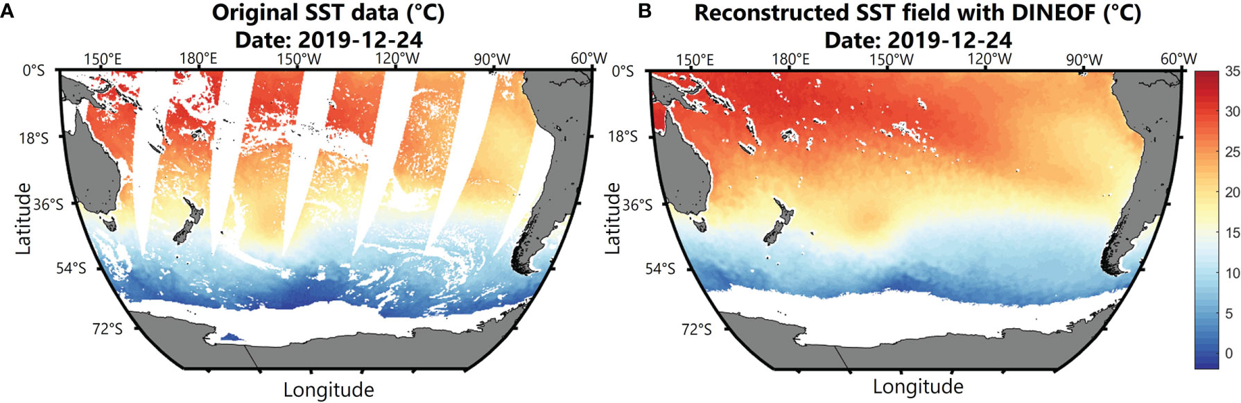
Figure 2 (A) AMSR-2 sea surface temperature (SST; °C). White parts indicate the missing data due to rain, ice and satellite limitations (swaths). (B) Reconstructed SST (°C) with DINEOF. Missing data are still present alongshore and everywhere water was covered at least one day by sea ice.

We reconstructed the whole South Pacific Ocean but decided that every portion of water covered at least one day by sea ice will not be part of the reconstruction, as we are not interested in high latitudes. For each year (2012-2020), the percentage of missing data in the original SST dataset for the whole South Pacific was between 35% and 37%. For the reconstruction, 50 EOF were calculated by DINEOF for each year, explaining in average 99.89% of the initial variance. To estimate the accuracy of DINEOF reconstruction, we calculate the bias, correlation and root mean square error (RMS) between the reconstructed field and in situ data from drifting buoys (shown in Table 1). We used 10 surface drifting buoys with hourly temporal resolution (allowing to select the same hour at which the satellite measures of the SST were done), all scattered offshore Central and South Chile between the coast and about 2 500 km offshore, with a complete temporal coverage from 2014 to 2020. In total, 4219 points were used to estimate the accuracy of our reconstruction (buoys’ data are available at https://map.emodnet-physics.eu/). Results show a slight negative bias which indicates that the satellite and the reconstructed SST are lower than the in situ SST. The bias, the correlation and the RMS are very close for both sets of data, meaning that our reconstructed field is as accurate as the satellite data.

TABLE 1

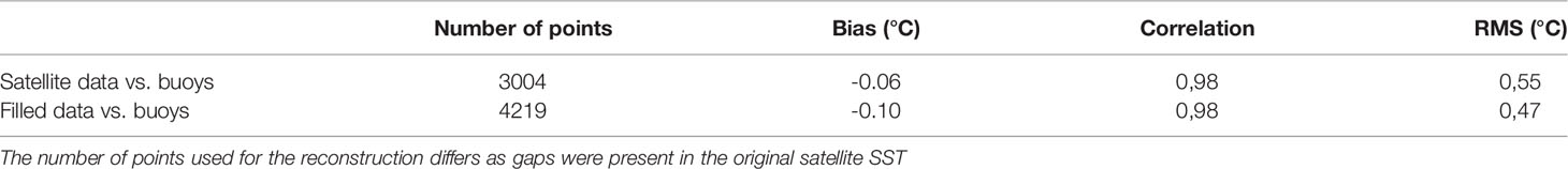
Table 1 Bias (°C), correlation and root mean square error (RMS, °C) calculated between original satellite SST and SST from in situ buoys and between the reconstructed SST field with DINEOF and the SST from the buoys.

2.4 SST Trends

We calculated the seasonal mean SST over the studied area by doing the long-term average (1982 to 2020) over austral summer, autumn, winter and spring. To calculate the SST long-term trends, as a first step we removed SST seasonal variation to our SST values through a low-pass filter in order to have only the annual SST trends and removed seasonal variations. Then, SST linear trends were calculated from 1982 to 2020, by using the OISSTv2 dataset. We choose p-value inferior to 0.05 as a significant trend. Secondly, trend calculation was performed again over ten-year periods, from 1982 to 1991, 1992 to 2001, 2002 to 2011 and 2012 to 2020.

2.5 Marine Heatwaves

In this study, we used the MHW definition given by Hobday et al. (2016), which defines MHWs as continuous events of warm SST anomalies exceeding a threshold (90^th percentile with respect to a 30-years climatology) during at least 5 days. Our marine heatwave detection is based on the HeatwaveR algorithms provided by Schlegel and Smit (2018) available at https://robwschlegel.github.io/heatwaveR/index.html. The SST is spatially averaged over a determined area (in our case Northern, Transition and Southern areas) and the algorithm determines when MHWs are occurring, calculating for each day a long-term climatology, a threshold according to this climatology (90^th percentile), and find the periods during which SST exceed this threshold during at least 5 days with no more than 2 below-threshold consecutive days, based on a 11-days moving mean centred on each Julian day (in the case of time series SST data) or on each pixel (in the case of gridded data). In addition to the MHW calculation, the algorithm provides several metrics: number of events per year, duration of each event and maximal and mean intensity (the maximal intensity is the highest temperature anomaly value recorded during the MHW whereas the mean intensity is the mean temperature anomaly observed during the event).

To calculate the climatology, Hobday et al. (2016) recommend to have at least 30 years of SST data because multi-year cyclic events (e.g. ENSO) must be considered to calculate the MHWs. Here we used the same dataset as they did, that is to say the OISSTv2 dataset but over a longer period, from 1982 to 2020. The threshold we used to calculate MHWs is the 90^th percentile. In addition, the algorithm also determines the long-term trends in MHW occurrence by first calculating the number of MHW in each pixel of the gridded data that has occurred, in our case between 1982 and 2020, and then applying a generalised linear model to each pixel. From the generalised linear model, slope and p-value (<0.05) are used to determine the long-term trends in MHW occurrence.

Hobday et al. (2018) have proposed a classification of the MHW events in order to have a better visualisation of the MHWs’ real impact on ecosystems. This classification has 4 categories which depend on the maximal intensity reached by the MHW event (which in turn depends on the climatology). Categories are based on multiples of the local difference between the climatology and the threshold. Between 0 and 1 times the differences between the climatology and the threshold, no MHW is detected; between 1 and twice the difference it is a Category I MHW, between 2 and 3 times the difference it is a Category II MHW, Category III corresponds to 3 to 4 times the difference and a Category IV corresponds to more than 4 times the difference. This categorization is also given by the heatwave detection algorithm.

3 Results

3.1 Marine Heatwaves in Central and South Chile: 39 Years of Data

To understand how MHWs have evolved within a 39-year period, we performed an analysis of the duration and intensity for each event and studied the number of MHWs occurring each year. MHWs were identified by doing the spatial average of the SST within the 3 studied areas and their metrics were identified using HeatwaveR code.

From 1982 to 2020, the Northern, Transition and Southern area experienced respectively a total of 75, 73 and 71 periods under MHW conditions from which 5, 6 and 9 MHW periods had a duration superior to one month. In the Northern and Transition areas, the highest number of MHWs was recorded during El Niño years, respectively 9 events in 1997 and 7 in 1998 (Figures 3A, B). For the Southern area, in both 1987 and 2020, 6 MHWs were recorded of which 3 had a duration superior to 1 month (Figure 3C). For the Transition area, alternance of years with and without MHWs was common until 2011 (Figure 3B). Nonetheless, from 2011 to 2020, MHWs were recorded every year totalling during that 10-year period 45% of all MHWs recorded for the area. The decade 2012-2020 was particularly active in terms of number of MHW events for the Transition area, totalling on average twice as many events than during the 1982-1991 decade and was 2.5 times superior to the number of events that have occurred during decades 1992-2001 and 2002-2011 (Figure 4E). It is notable that the early 21^st century was MHWs-free for all 3 areas (this period was the longest in the Transition area).

FIGURE 3

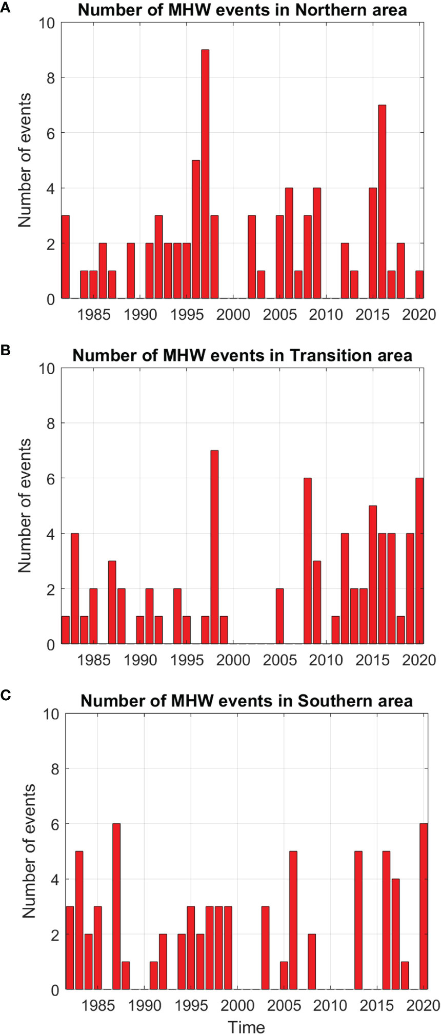
Figure 3 Number of marine heatwave events (MHW) that have occurred each year from 1982 to 2020 for Northern (A), Transition (B) and Southern (C) areas.

For all 3 areas, the mean duration of MHWs for the 1982-1991 decade was about 10 days and was the lowest of the four decades (Figure 4A), whereas mean duration during the 2012-2020 decade was the longest recorded, with 20 days, 19 days, 23 days for respectively Northern, Transition and Southern area (Figure 4B). The mean duration was multiplied by 2.14, 1.9 and 2.3 respectively between the two decades. Between 1982-1991 and 2012-2020, the duration of the longest event has been multiplied by 8, 5 and 3 for respectively Northern, Transition and Southern areas. The longest event in the Northern area began in January 2017 and lasted for 137 days (4.5 months); in the Transition area, the longest event began in May 2016 and lasted for 148 days (almost 5 months), and in the Southern area, the longest event began in June 2016 and lasted for 119 days (almost 4 months).

FIGURE 4

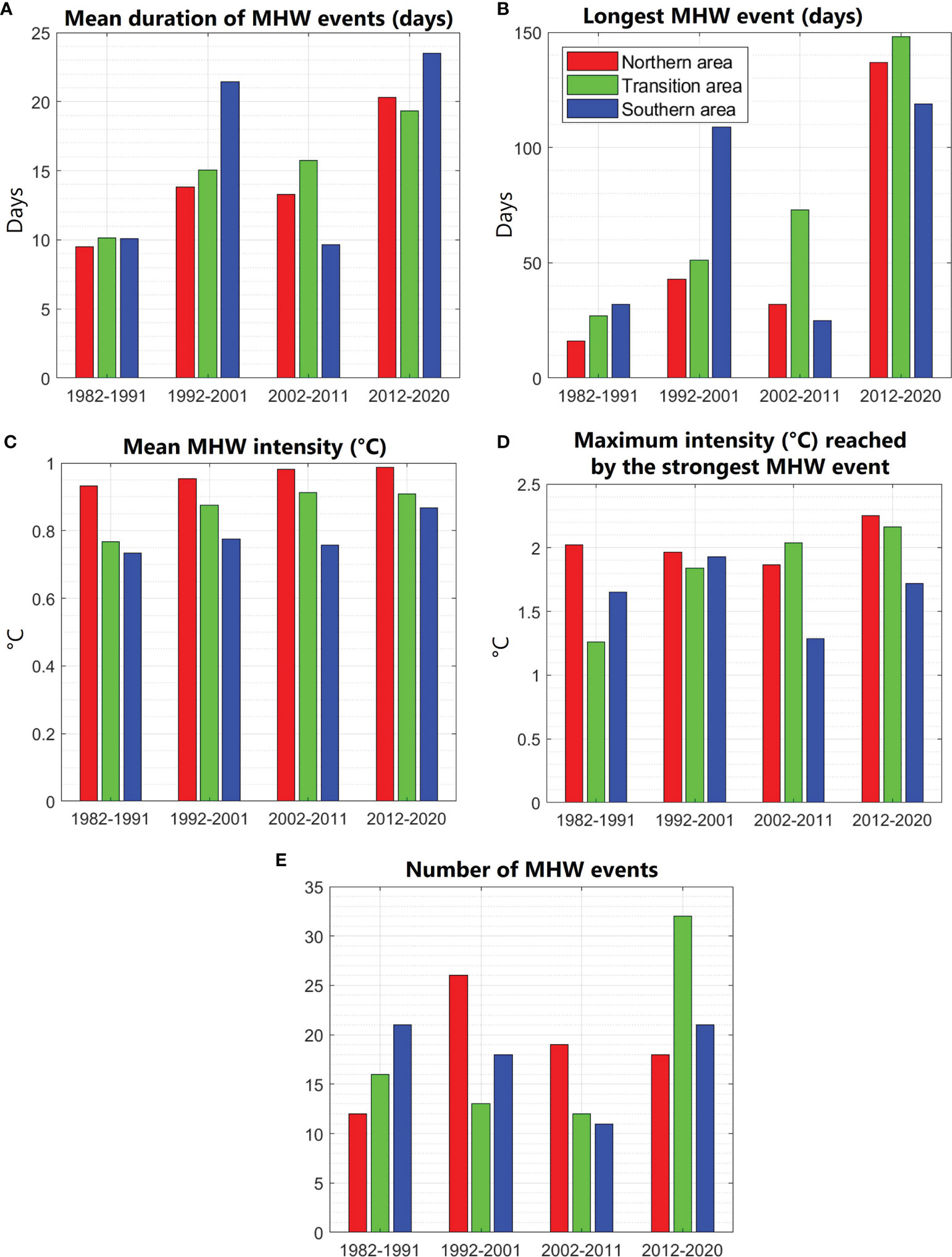
Figure 4 Decadal trends (1982-1991, 1992-2001, 2002-2012, 2012-2020) for Northern (red), Transition (green) and Southern (blue) areas. Parameters analysed over the different decades are: (A) mean duration (days) of the events that have peaked during the decade, (B) duration (days) of the longest event of the decade, (C) mean intensity (°C) of all the events that have occurred during the decade, (D) maximal intensity (°C) reached by the strongest event of each decade, (E) number of MHW events that have occurred throughout the decades.

Regarding the intensity over the decades, the mean intensity of the MHWs is the highest in the Northern area and the lowest in the Southern area (Figure 4C). For the Northern area, the strongest event recorded was in 2017 with a maximal intensity of 2.3°C (Figure 4D), classified as a Category III event. This strong event corresponds to the longest one recorded in this area (137 days). For the Transition area, the highest intensity recorded was 2.2°C corresponding to a Category II MHW which started in October 2016 and lasted for 64 days. In the Southern area, the strongest event ever recorded was a Category II event in 1998. It occurred while a strong El Niño event was present and had a maximal intensity of 1.9°C with a duration of 99 days. It seems interesting to note that the strongest event recorded was during the last decade for both Northern and Transition areas. Indeed, 21%, 40% and 38% of the MHW events (respectively for Northern, Transition and Southern areas) that had a maximal intensity superior to 1°C occurred after 2011 whereas it represents only a fourth of the total period we studied. In the same way, 36%, 33% and 50% of the events (respectively for the Northern Transition and Southern areas) having a maximal intensity superior to 1.5°C occurred after 2011.

3.2 Development of the MHWs in 2016-2017

The years 2016 and 2017 were particularly hit by MHWs with, from May 2016 to May 2017, 219, 298 and 224 days under MHWs conditions for respectively Northern, Transition and Southern areas. More specifically, from May to December 2016 (that is to say a duration of 245 days), the Transition and Southern areas were under MHW conditions during respectively 212 and 216 days (and “only” 86 days for the Northern area). Those conditions were caused by a succession of unusually long and strong MHWs that started on May 2016 (see details in Figure 5).

FIGURE 5

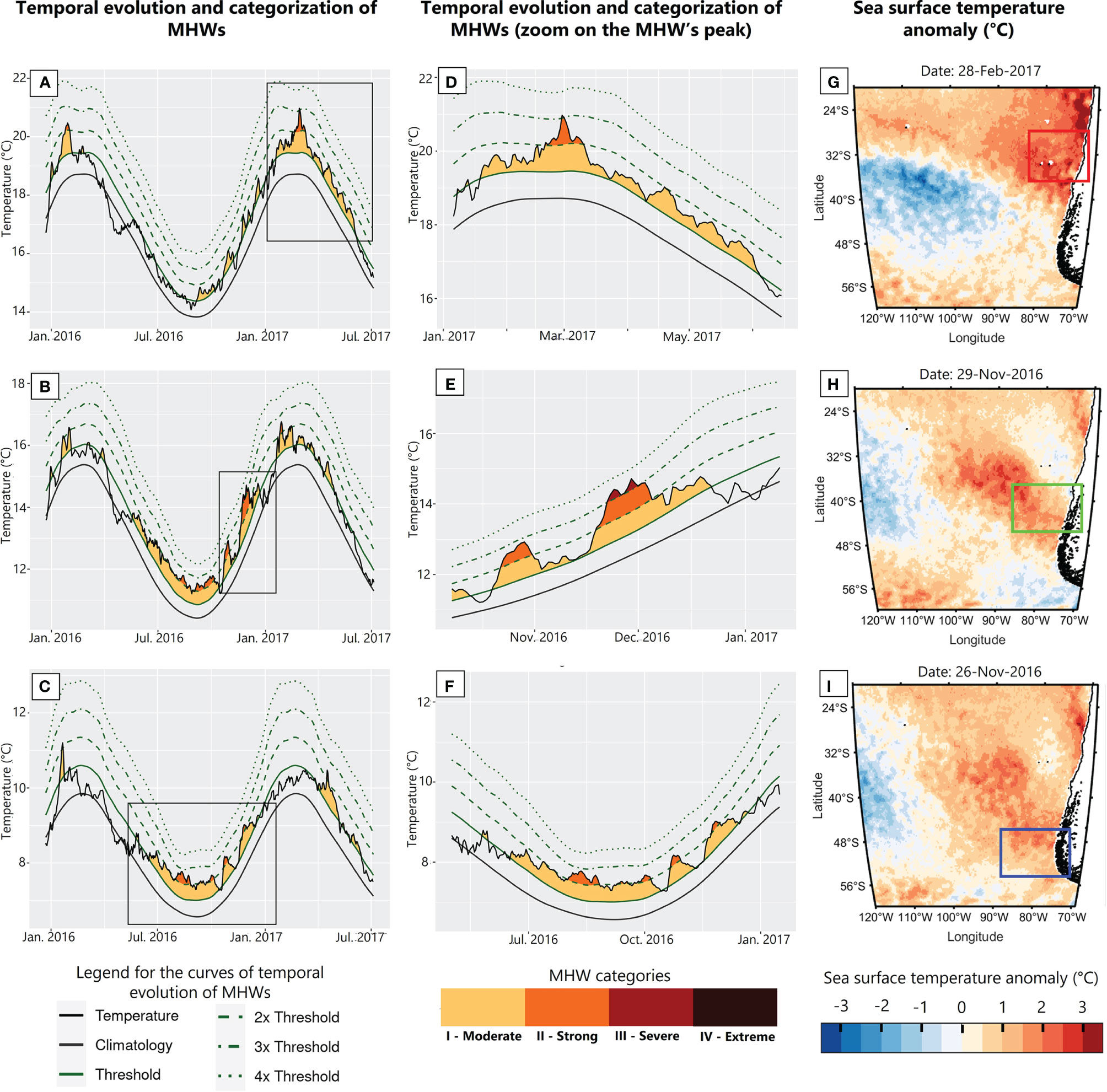
Figure 5 Temporal evolution of the marine heatwaves (MHWs) recorded between January 1^st of 2016 and July 1^st of 2017 (A–C). Those graphs are obtained by averaging the sea surface temperature (SST) over the corresponding area. (D–F) Represents a zoom over the strongest event recorded for each area over this period, highlighted by the black square in the left column. For both left and central columns, the lower line of the graph (black and bold) represents the long-term climatology. The irregular black line represents the daily SST temperature. The green bold line represents the threshold, the first green dashed line is 2 times the threshold, the second green dashed line represents 3 times the threshold and the final green dashed line represents 4 times the threshold. The MHWs categorization is represented by the colours with yellow, orange, red and dark purple corresponding respectively to Category I, II, III and IV. (G–I) Represents the SST anomaly on the day of the main peak of the strongest event. The areas are represented by the coloured squares. Upper line corresponds to the Northern area, middle one to the Transition area and bottom one to the Southern area.

On May 19^th 2016 (austral fall) started MHW conditions in the Transition area and one month later, on June 17^th, in the Southern area. The MHW peaked on June 29^th (austral winter) in the Transition area with a maximal intensity of 1.4°C and on August 18^th in the Southern area with a maximal intensity of 1.1°C. For both areas, the MHW was considered as a Category II event. On October 13^th (austral spring), the MHW disappeared for both areas resulting in 148 days under MHW conditions for the Transition area and 119 days for the Southern area. However, only 7 days later, on October 20^th, a new MHW started again in both areas. That time, the intensity of the MHW decreased quickly in early November, the MHW conditions almost disappeared for the Transition area and even disappeared in the Southern area on the 9^th of November. Nevertheless, the MHW’s intensity increased back by mid-November, provoking a new MHW for the Southern area with a maximal intensity of 1.2°C and for the Transition area the strongest intensity reached over the last 39 years with a value of 2.2°C on November 29^th. The MHW then progressively disappeared by the end of December. Finally, MHW conditions totalled 64 days of uninterrupted MHW conditions in the Transition area and 55 days for the Southern area interrupted by 9 days without MHW conditions in November. The MHWs were Category III events for the Transition area and Category II for the Southern area. Concerning the Northern area, 4 relatively short (inferior to one month) and weak MHWs were recorded in austral spring 2016, from September to December. All were Category I events except the third one which was a Category II event with a maximum intensity on November 24^th of 1.5°C. Then, on January 19^th of 2017 began a Category III MHW which lasted for 137 days with a maximal intensity of 2.3°C on February 28^th, being the longest event recorded for the Northern area and the strongest one of all areas combined. At the same period, the Transition area experienced discontinuous short (inferior to 1 month) and weak (all Category I events) MHWs from January to March 2017.

3.3 Atmospheric Conditions in 2016-2017

In April 2016, a high-pressure system was present in the extreme South Pacific Ocean, reaching Chilean coasts up to 45° S (Figure 6A). In May and June, the high-pressure system moved northward, encompassing the whole Patagonia and reaching the highest pressure ever recorded over the 2012-2020 period for both Transition and Southern areas (Figures 6B, C). This resulted in very stable anticyclonic conditions over the Transition and Southern areas, leading to a low winds velocity, the lowest recorded over the 2012-2020 period for all 3 areas (Figures 7A–C). Furthermore, in the Transition area, the east-component of the wind speed is fully eastward over the 2012-2020 period except in mid-May 2016, having a very low wind speed with a westward direction. During austral winter, the high-pressure system moved toward eastern Patagonia and disappeared in August.

FIGURE 6

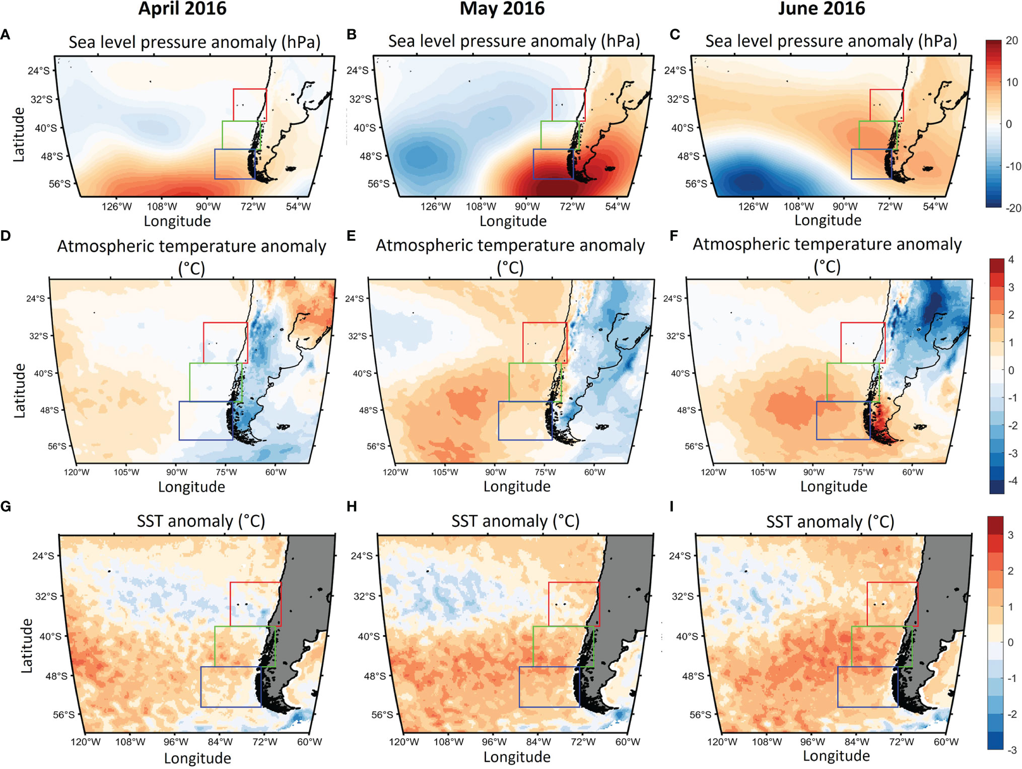
Figure 6 Monthly average sea level atmospheric pressure anomalies (A–C), atmospheric temperature anomalies (D–F) and sea surface temperature (SST) anomalies (G–I), expressed respectively in hPa, °C and °C, for the months of April 2016 (left column), May 2016 (central column) and June 2016 (right column). Colour scale is indicated on the right side of each line. Areas concerned are all located between 20°S and 50°S, and between 50°W and 140°W for pressure anomaly, between 60°W and 120°W for air temperature anomalies and between 60°W and 120°W for SST anomalies.

FIGURE 7

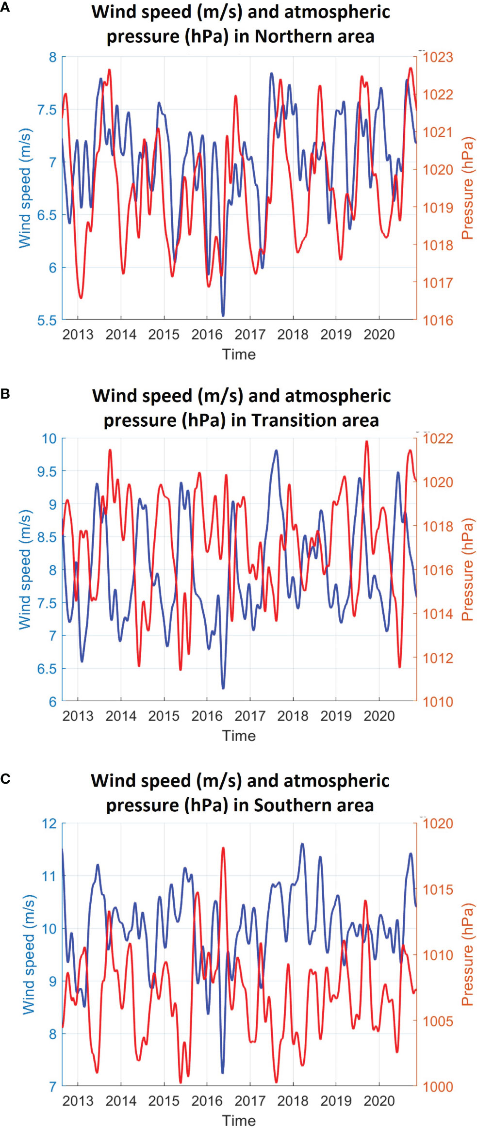
Figure 7 Wind speed (blue) and sea level atmospheric pressure (red) from 2012 to 2020 for Northern (A) Transition (B) and Southern (C) areas. A 3-month Gaussian filter was applied to the data. For a better visualisation of the variations, y-axis’ scales differ.

SST and air temperature were evolving in similar ways. In April 2016, at midlatitudes, a large patch of SST anomalies is present offshore Chile, affecting both Transition and Southern areas (Figure 6G). A core of negative SST anomalies was observable between the mid-latitude warm patches and warm anomalies at tropical latitudes. The same pattern is observable for atmospheric temperature anomalies (Figure 6D). In May, the SST patch moved eastward (Figure 6H), bringing warm anomalies nearshore. Those anomalies were the highest in the Transition area with local anomalies between 2°C and 2.5°C. Alongshore, the warm anomalies merged with lower latitude anomalies, forming a continuous band of positive anomalies along Chilean coasts. Again, a similar distribution of warm atmospheric temperature anomalies is observed (Figure 6E). In June, the air temperature anomalies were still high and the patch of warm SST anomalies was still getting closer to Patagonian coasts (Figures 6F, I). Although the SST anomalies persisted during austral winter, they were progressively diminishing until early spring. However, in October, a patch of warm air temperature anomalies formed in the tropical Pacific, moving progressively southeastward, reaching in November the Juan Fernández Archipelago. In early November, a very warm circular patch formed in the ocean, coinciding with the location of the warm air patch, centred approximately on 90° W and 35° S, West of Juan Fernández Archipelago. At this place, the temperature anomalies rose quickly, reaching on November 18^th 4.5°C for the SST and 4°C for the air temperature (Figure 8); no remarkable positive or negative pressure system was observed where the patches were present. Then, both warm SST and warm air patch migrated southeastward, losing in intensity, and reached coasts of the Transition area in late November. The warm SST patch progressively disappeared in December but pulsed again South-West of Juan Fernandez Archipelago in early 2017. The warm air patch was still present in January and February affecting at that time only the Northern area.

FIGURE 8

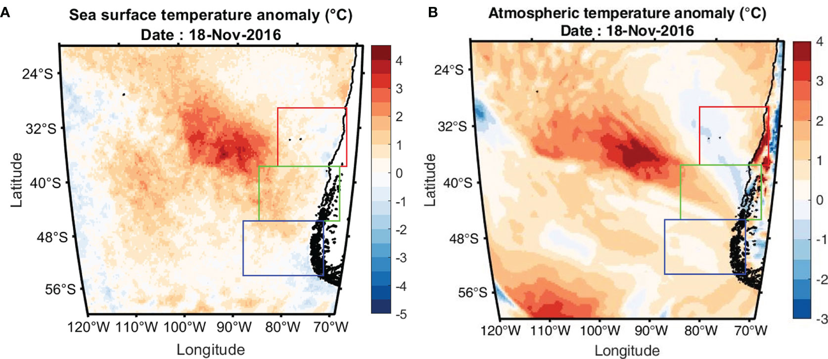
Figure 8 (A) Sea surface temperature anomaly and (B) air temperature anomaly (both in °C) on November 18^th, 2016. A particularly warm patch is observable, centred on 90°W 35° S, with anomalies reaching locally 4.5°C for the SST and 4°C for the air temperature.

In addition to the atmospheric variables, we also analysed the mean heat transfer from the ocean to the atmosphere over the period 2012-2020 (Figure 9). Indeed, during late fall and winter 2016, offshore Chilean coasts, the heat transfer from the ocean to the atmosphere was lower than usual, being reduced up to 100 W/m² in June in both Transition and Southern areas compared to the 2012-2020 average (Figure 9C). This diminished heat transfer was caused by a lower latent and sensible heat transfer. Indeed, in the Transition area the latent heat was reduced by 1/4 in May and June, while in the Southern area it was reduced by ~1/3 from May to July. The sensible heat was reduced in the Transition area from May to September, being reduced up to 1/3 from June to August, whereas in the Southern area a reduction is observed from May to September being almost equal to zero in June and divided by 4 in July. By the end of austral spring, the heat transfer slightly recovers to normal values except in November when the warm SST and air patches were observed.

FIGURE 9

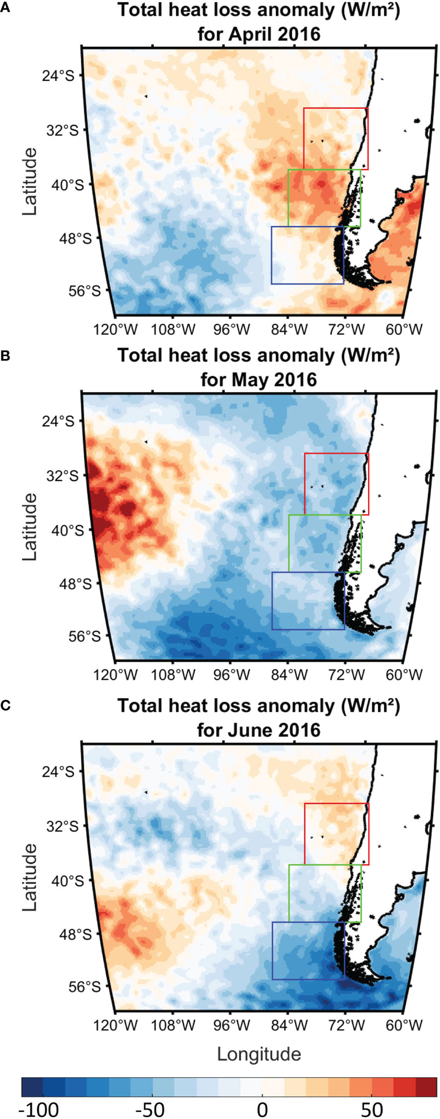
Figure 9 Monthly anomaly of total heat transfer (in W/m²) from the ocean to the atmosphere for (A) April, (B) May, and (C) June of 2016. The anomaly has been calculated according to the 2012 to 2020 average.

4 Discussion

SST satellite products covering the period of 1982-2020 were used in this manuscript to understand the forcing mechanisms involved in the formation of MHWs offshore central and south Chile. The data analysis showed an increase in MHWs events during the last decade, particularly offshore Northern Patagonia. On another side, the years of 2016-2017 were significant in MHWs occurrence, in terms of duration and intensity. Detailed descriptions of the main results are included in the following discussions sections.

4.1 SST and Marine Heatwaves Trends

SST trends from 1982 to 2020 show that the Central South Pacific has been particularly hit by warming waters during the last 39 years (Figure 10A). A very large patch from the Tropics to mid-latitudes suffered from positive trends, about 0.03°C per year within the patch’s centre. The patch reaches South American coasts from 30°S to 47°S, except at 37°S where a cold trend is present. According to those trends, the Transition area is the only South American Pacific coast (South of 10°S) impacted by positive trends, ranging from 0.005 to 0.015°C per year. A closer look to the decadal trends confirms that Chilean coast did not suffer from warming trends during the three first decades (cooling trends are observed nearshore), although a tongue-shaped positive trend is observable in the open ocean centred approximately on 35°S (Figures 10B–D). Nevertheless, the last decade shows a totally different pattern, with positive anomalies everywhere (except a horseshoe pattern of negative trends), particularly high along Patagonian coasts with trends of +0.05°C to +0.1°C per year (Figure 10E). Note that the Central South Pacific has been badly hit during all 4 decades. The long-term trends are consistent with what was observed by Roemmich et al. (2016): a tongue-shaped warm patch, with a warm core between 30° S and 40° S getting closer to the coast between 38° S and 47° S. However, contrary to what we found, Roemmich et al. (2016) highlight cooling trends nearshore. The difference might be linked to the different time series used: their study has been realised from 1981 to 2015, whereas our study also encompassed the end of the last decade which was important in terms of warming. In addition, Gutiérrez et al. (2018) found that winter SST has been increasing from 2010 to 2016 in Northern Patagonian fjords, being maximal in 2016, the winter we observe the very long MHW in both Transition and Southern areas.

FIGURE 10

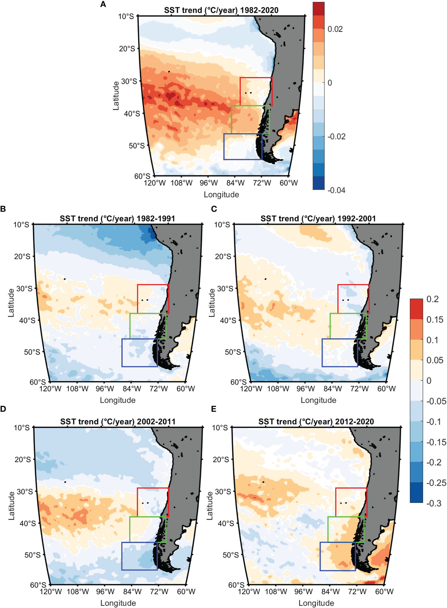
Figure 10 Significant sea surface temperature (SST) trends (according to pvalue<0.05) in °C per year for (A) 1982-2020, (B) 1982-1991, (C) 1992-2001, (D) 2002-2011 and (E) 2012-2020. Areas where no significant trends were observed are shown in white.

HeatwaveR algorithms can also provide the MHWs trends (Figures 11A, B). Thus, we performed the analysis over a reduced portion of the Southeast Pacific Ocean from 1982 to 2020, focusing only on our 3 areas of interest. The results are the MHWs frequency trends within each pixel. An increase of the MHWs frequency is remarkable at mid-latitudes, especially at lower latitudes than 46° S. Along Transition area coasts, a positive trend is also present but not significant. Moreover, a negative trend is observable at 37° S, at the location of the Punta Lavapie upwelling system. The same distribution pattern of MHWs trends and SST trends can be explained by the fact that MHWs are highly related to increasing SST across the globe (Frölicher et al., 2018).

FIGURE 11

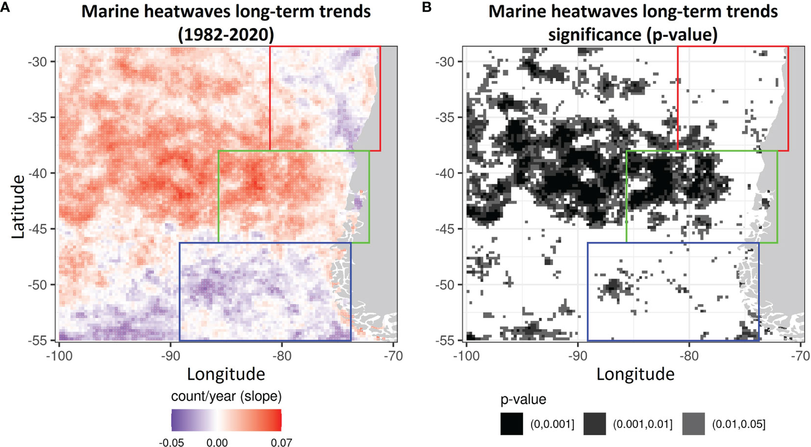
Figure 11 Marine heatwaves (MHWs) trends (A) and significance of the trends according to the p-value (B). The trend is calculated according to the number of MHWs that have occurred in each pixel from 1982 to 2020. Consequently, a positive (negative) trend significate that the number of MHWs is increasing (decreasing) with time.

4.2 Formation and Processes of the 2016-2017 MHWs

In autumn 2016 started a series of MHWs in the Southeast Pacific Ocean, offshore South Chilean coasts (Figure 5). In April 2016, positive SST anomalies coming from the extratropical Pacific (~55°S, 130° W) started to be stronger in the Transition area, accompanied with diminishing winds (Figure 6G). This warm patch observed in the extratropical South bringing positive SST anomalies to Patagonia through the Pacific Gyre could be part of the South Pacific Ocean Dipole. This dipole is composed of an extratropical positive SST anomalies patch (which would corresponds to the one we highlighted) centred on about 58° S, 125° W and a subtropical negative SST anomalies patch centred on the eastern coast of New-Zealand (Saurral et al., 2020). The main variability of the dipole is explained by ENSO (Li et al., 2012; Chatterjee et al., 2017): the warm anomalies in the extratropical dipole are enhanced when positive phases of ENSO are occurring. Strong El Niño conditions were present in austral summer 2015-2016 (Figure 12A), probably strengthening the dipole’s warm anomalies. In addition, dipole’s SST anomalies are subject to eastward propagation (Li et al., 2012) explaining why they reached Patagonia. In May 2016, the wind speed reached its lowest value over the 2012-2020 period for both Northern and Southern areas (Figure 7), and the Transition area experienced unusual westward winds. The combination of unusually weak winds due to a persisting high-pressure system (the highest recorded for the Southern area over the period 2012-2020) reducing the heat loss from the ocean (sensible and latent heat; Figure 9) and the presence of anomalously warm waters triggered MHW conditions in the Transition area in mid-May. In June, the SST anomaly, still coming from the extratropical ocean (Figure 6I), got stronger in the Southern area, allowing to trigger MHW conditions in that area by the end of the month (Figure 5F). We did not perform a comparison between 2016 wind speed and long-term wind speed, but Garreaud, (2018a) did it off Chiloe Island (42.5°S, 74.3°W, located in the Transition area) and shown that winds were about twice inferior to the long term average from late-May to mid-June. In winter, the wind gets back to usual values, and the heat transfer from the ocean to the atmosphere progressively gets back to normal by early spring. In spring, SST anomalies were present but were getting lower than during previous months, barely maintaining MHW conditions. The MHWs conditions stopped by mid-October in both Transition and Southern areas, totalling 148 days under MHWs conditions in the first area and 119 in the second one (Figure 5). The Northern area has not been affected by this MHW, except in the form of short heat peaks during winter. However, advection of warm waters coming from extratropical South Pacific triggered new MHWs in all 3 areas in mid-October but were not high enough to maintain the MHW conditions resulting in early November in a break within the MHW period in Northern and Southern areas and to its almost disappearance in the Transition area. Meanwhile, a warm patch formed very quickly in both ocean and atmosphere West of Juan Fernández Islands in early November 2016 (Figure 8), with an SST anomaly increase of 2.5°C in only 12 days. Both atmospheric and oceanic warm patches moved southeastward and reached the coasts in late November, encompassing the three areas and coinciding with the new apparition of MHW conditions in Northern and Southern area and to the strengthening of the MHW in the Transition area. In the Transition area, this MHW corresponds to the most intense one recorded over the 1982-2020 period. In the Northern area, the MHW was not that strong because of the presence of a coastal negative anomaly signal at approximately 37°S, corresponding to Punta Lavapie, an area where upwelling favourable winds are predominant from September to February (Letelier et al., 2009), explaining the negative SST anomalies often observed in this area. However, the positive anomalies patches got cooler while moving northeastward in mid-December and the anomalies were decreasing. Nevertheless, in late January 2017, both SST and atmospheric temperature anomalies patch increased back, provoking the 137 days (4 and a half months) MHW in the Northern area (which was, by the way, the strongest event ever recorded along Chile) and to short pulses in Transition and Southern areas.

FIGURE 12

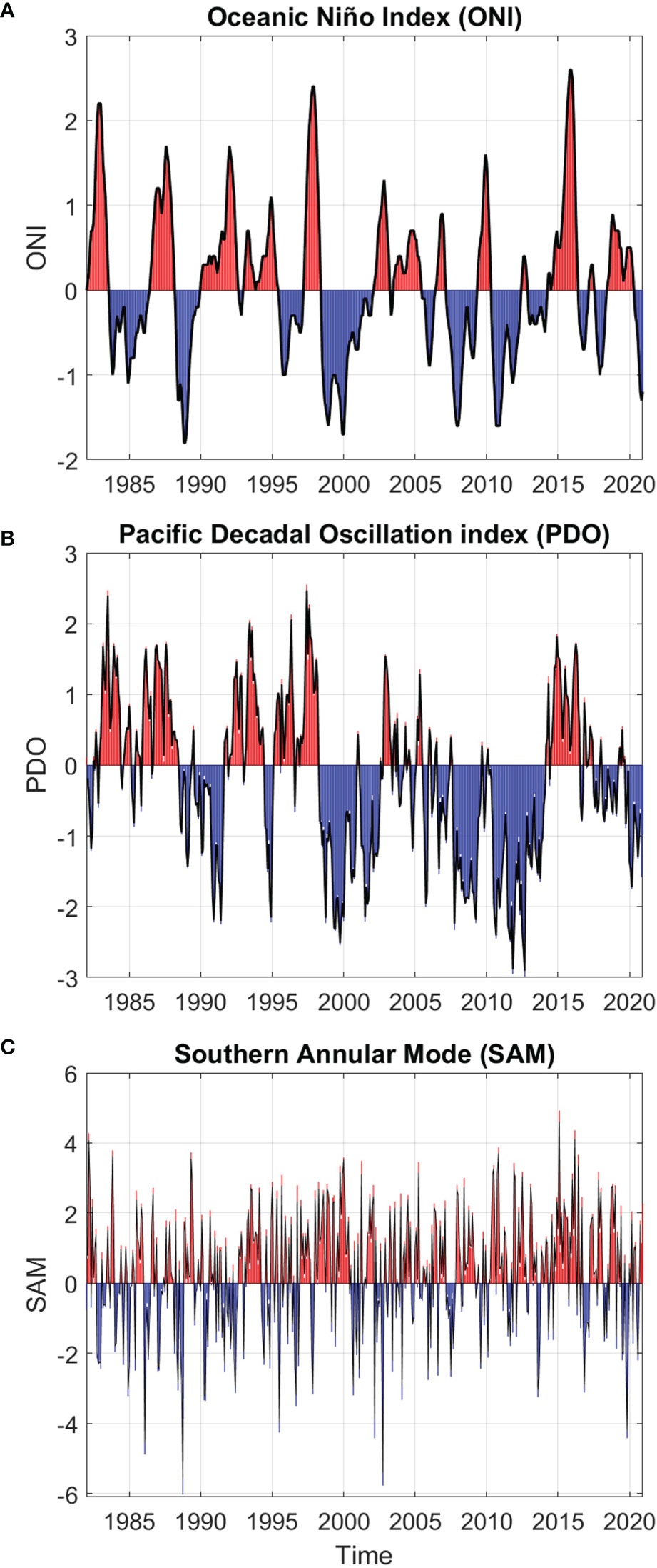
Figure 12 Different remotes forcings expressed by their index. (A) Oceanic Niño Index for ENSO monitoring (ONI), (B) Pacific Decadal Oscillation (PDO) index, (C) Southern Annular Mode (SAM) index. Red indicates a positive period and blue a negative period. PDO and SAM index are expressed with a 3-month Gauss filter, represented by the black bold line. ONI calculation is already based on a 3-month average. The scale differs according to the index.

It is important to note that in the part of the world we are interested in, SST is generally higher than the air temperature. To understand how SST and air temperatures are related, we spatially averaged SST anomalies and air temperature anomalies (and applied a 3-months Gaussian filter on both) over the period 2012-2020 for the 3 areas and calculate their correlation to know how they are related. Over the period 2012-2020, the correlation between air temperature anomalies and SST anomalies was the highest with a 10, 1 and 3-days lag respectively for Northern, Transition and Southern areas. The correlation was therefore 0.9291, 0.8748 and 0.8711 respectively. However, having a more specific look to the year 2016 only, air temperature and SST anomalies were occurring with no lag for both Northern and Transition areas, whereas for the Southern area, SST anomalies were leading air temperature anomalies by 9 days; correlation between the two parameters for all 3 areas being higher than 0.94 for the year 2016. Consequently, as the SST is higher than the air temperature and as SST variations precede or occurred at the same time as air temperature variations, this would signify that the autumn-winter-spring MHWs in 2016 were not led by the air temperature. However, the global atmospheric conditions (lower winds associated with high-pressure system, thus reducing heat loss from the ocean) contribute to enhance the SST anomalies, preventing waters to cool during winter, in addition to the warm waters advected from the South-Central Pacific Ocean. That combination of oceanic and atmospheric factors, i.e. advected warm waters, high pressure system inducing reduced winds and in return a decrease in the sea-air fluxes, having led to MHW formation has already been observed in the past, for instance in the Pacific Ocean when a MHW lasted from 2013 to 2015 (Bond et al., 2015) or in 2011 in Western Australia (Pearce and Feng, 2013).

Besides the oceanic and atmospheric forcings, remote forcings could have played a role within the longevity and intensity of the MHWs events during 2016 and 2017. Indeed, in 2014, ENSO switched to a positive phase until mid-2016, being one of the three strongest El Niño events ever recorded with the 1982-1983 and 1997-1998 ones (Figure 12A). Because of its importance, it has been popularly named “Godzilla El Niño”. Garreaud, (2018b) has shown that the Godzilla El Niño event, was associated with strong positive sea level atmospheric pressure anomalies (>5 hPa) at extratropical latitudes during austral summer 2016. In our study, we found that during austral autumn (March-April-May), the atmospheric pressure anomalies were also high, with seasonal average up to 10 hPa. In addition, the warm patch we described West of Juan Fernández Archipelago that formed in November 2016 and strengthened in January 2017 was probably linked to a “coastal El Niño” (Garreaud, 2018b; Rodríguez-Morata et al., 2019; Smith et al., 2021), whose characteristics were a strong and rapid warming of the easternmost Equatorial Pacific in January 2017 followed by other warm pulses in February and March, associated with very weak Tradewinds from January to April 2017 (Garreaud, 2018b). In fact, the whole Central Pacific experienced a very strong El Niño in 2015-2016 and the easternmost Central Pacific experienced a coastal El Niño in summer 2016-2017 (Garreaud, 2018b). In its study, Garreaud, (2018b) highlights a tongue-shaped warm SST coming from Equatorial Pacific and extending southeastward to the coasts of our Northern area, in accordance with what we described. This warm patch resulted in the formation of the most intense MHW in the Northern area, which lasted from January 19^th to June 4^th 2017. In addition to the El Niño event, a positive phase of PDO also occurred from 2014 to 2017 (Figure 12B). PDO has already been correlated with positive sea surface temperature for the period 2014-2017 in previous study (Narváez et al., 2019). Indeed, when its positive phase occurs together with ENSO’s positive phase, their consequences can cumulate and cause lower winds and warmer conditions at mid-latitudes (Garreaud et al., 2009; Ancapichun and Garcés-Vargas, 2015; Yáñez et al., 2017). Besides the El Niño and PDO events, a strongly positive phase of SAM also occurred in 2016 (Figure 12C). Nevertheless, usually ENSO and SAM have negative correlation (Gong et al., 2010), thus the synchronisation of very strong positive events of both phenomena seems confusing. However, as the two phenomena have the same consequences over Chilean Patagonia, meaning high pressure systems South of Patagonia, reduced Westerly winds at mid-latitude and higher temperatures, their combined effects might exacerbate their consequences. And effectively, the drop in wind speed we observed in late autumn 2016 and the high pressure associated were the highest ever recorded at least over the period 2012-2020. Although SAM has been cited in a few studies as a factor maintaining or initiating environmental conditions for MHW formation (e.g. Perkins-Kirkpatrick et al., 2019; Salinger et al., 2019; Su et al., 2021), its implication within the formation of MHWs, particularly in the Southeast Pacific Ocean, needs to be in-depth investigated.

4.3 Marine Heatwaves Consequences on Fjords Ecosystems

Although Patagonian ecosystems are extremely vulnerable to global warming (Yáñez et al., 2017) and even if fjords are considered as aquatic critical zones (Bianchi et al., 2020), only few studies have been realised on MHWs’ consequences on fjords ecosystems and none on Patagonian fjords. Here, we suggest that numerous typical impacts of MHWs could be considered according to what has been observed in other parts of the world. For instance, a HAB occurred in North Patagonia inner seas from February to May 2016 (Garreaud, 2018a; León-Muñoz et al., 2018; Armijo et al., 2020) resulting in economic losses of several hundred million dollars (e.g. Díaz et al., 2019). HABs are often described as a consequence of MHWs (e.g. NOAA Climate, (National Oceanic and Atmospheric Administration Climate)2015; Roberts et al., 2019), but this one occurred shortly before the MHW we detected in the Transition area. That temporal mismatch could be due to the coarse spatial resolution of the SST data we used to perform our MHWs detection, preventing us to know if the inner seas experienced more numerous or longer MHWs than the open ocean did and if the HAB coincided with a MHW event. Another type of consequences of MHWs on Patagonian fjords could be the diminution of oxygen concentration. Indeed, Patagonian fjords are already experiencing hypoxic conditions due to fjord alimentation by low-oxygenated Equatorial Subsurface water mass filling the deep micro-basins (Silva and Vargas, 2014; Pérez-Santos et al., 2018), a strong stratification which prevents deep waters to be re-oxygenated by vertical mixing (Silva and Vargas, 2014) and anthropogenic activities (Silva and Vargas, 2014). The presence of a long-lasting and severe MHW as the one we observed during winter 2016 could worsen the hypoxic conditions by increasing thermal stratification and reducing oxygen dissolution (Breitburg et al., 2018), as it has already been observed in Norwegian deep-fjords where hypoxic conditions were exacerbated by deep waters warming, then affecting benthic communities (Aksnes et al., 2019). In addition, Patagonia is also a place for large aquaculture development, particularly salmon farming as the environmental conditions are optimal with average temperatures up to 15°C in summer for Northern Patagonia (Figure 13A). However, in February 2017, the strongest ever MHW event was recorded and SST nearshore was nearly 2°C higher than average, reaching 17°C (Figure 13B) in northernmost Patagonia, being close to the upper limit of optimal temperature growth for Atlantic salmons (Elliott and Elliott, 2010). Finally, decreases in microbial richness have already been observed in Patagonian fjords, associated with seasonal increase of sea temperatures, particularly in winter (Gutiérrez et al., 2018). This would probably be exacerbated as MHWs are projected to be more numerous, as we saw in section 4.2.

FIGURE 13

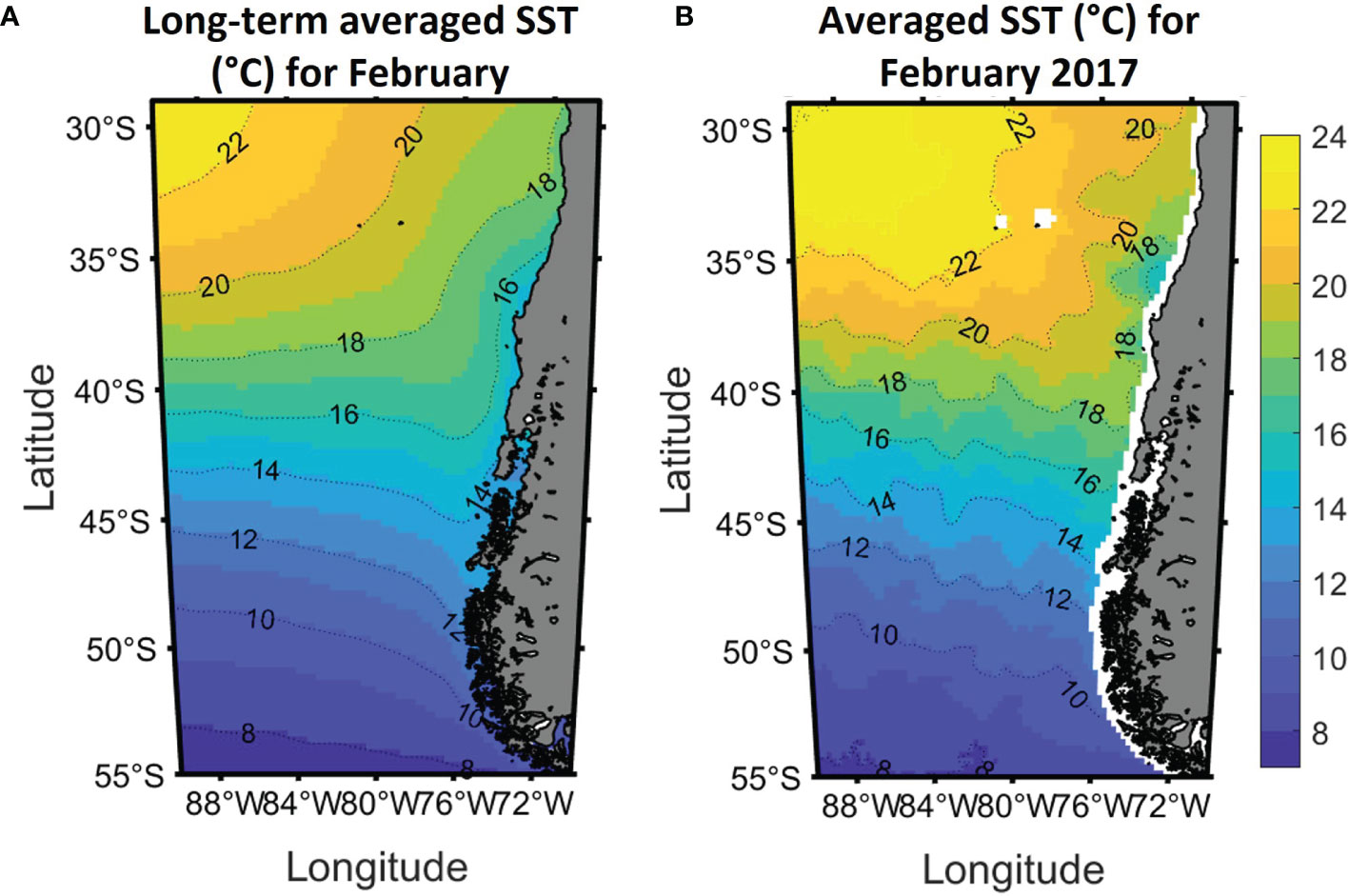
Figure 13 (A) Sea surface temperature (°C) long-term monthly averaged over 1982 to 2020 period for February and (B) monthly average for February 2017.

5 Conclusion

This study presents, to the best of our knowledge, the first assessment of the marine heatwaves (MHWs) that have occurred along Central and South Chile (29° S-55° S) from 1982 to 2020. We found that, although MHWs were already present in the 1980s, their intensity and their duration has increased, particularly over the period 2012-2020 with record-breaking events. The central studied area (North Patagonia) located between 38° S-46° S is the only Chilean coastal area where a long-term positive trend of MHWs frequency is present, probably related to the SST long-term warming trends. Indeed, that area totals 45% of the MHW events and 40% of the events that had an intensity superior to 1°C during the 2012-2020 period, showing how badly the area has been hit during the last decade. More particularly, the period from austral fall 2016 to summer 2017 suffered a succession of unusually long and strong MHWs. From May 2016 to May 2017, North Patagonia suffered about 300 days under MHW conditions. We found that in fall and winter 2016, warm waters were advected from the extratropical Pacific Ocean to the Patagonian coasts, contributing to the MHWs triggered and that atmospheric conditions were optimal for MHW development. Indeed, in May and June 2016, winds were abnormally low contributing to the diminution of the heat lost by the ocean. The MHW conditions persisted until spring 2016 and progressively disappeared. However, in November, new MHW conditions started causing the strongest MHW we recorded which lasted until early June 2017 in Central Chile, probably linked to a coastal El Niño. In addition, in early 2016, very strong El Niño conditions were reported and were associated with positive phases of SAM, probably having influenced the environmental conditions that have led to very intense and long MHW events.

In this study we analysed the surface development of the MHWs. However, the evolution of the detected MHWs off the coast of Chile, with several MHWs happening sequentially with only a few days between them, indicates that the subsurface temperatures might stay high during longer periods of time, favouring the development of new MHWs in the surface more easily. Therefore, further works should be dedicated to the subsurface development of the MHWs which is also primordial as it will define the depth at which species will be affected by the warming. Additionally, further studies should assess how the inner seas of Patagonia are affected by MHWs. Indeed, MHWs consequences add to the already existing hypoxia and to global warming might severely damage fjords ecosystems and aquaculture production.

Data Availability Statement

The datasets presented in this study can be found in online repositories. The names of the repository/repositories and accession number(s) can be found in the article/Supplementary Material.

Author Contributions

CP: Main research, main writer. AA-A: Main contributor to the research, main supervisor of the work, main supervisor of the writing. IP-S: Contributor to the research, supervisor. AB: additional help for research and for writing. All authors contributed to the article and approved the submitted version.

Funding

This work benefits financial support of the F.R.S-FNRS (Fonds de la Recherche Scientifique de Belgique, Communauté Française de Belgique) through funding the position of AB and funding a FRIA grant. IP-S was funded by FONDECYT 1211037, COPAS Sur-Austral ANID AFB170006, COPAS COASTAL ANID FB210021, and CIEP R20F002.

Conflict of Interest

The authors declare that the research was conducted in the absence of any commercial or financial relationships that could be construed as a potential conflict of interest.

Publisher’s Note

All claims expressed in this article are solely those of the authors and do not necessarily represent those of their affiliated organizations, or those of the publisher, the editors and the reviewers. Any product that may be evaluated in this article, or claim that may be made by its manufacturer, is not guaranteed or endorsed by the publisher.

Acknowledgments

The authors would like to thank Dr. Robert Schlegel and Dr. Albertus Smit for providing the HeatwaveR codes and packages freely at https://robwschlegel.github.io/heatwaveR/. The Oceanic Niño index (ONI) and the Pacific Decadal Oscillation are provided by NOAA available at https://origin.cpc.ncep.noaa.gov/products/analysis_monitoring/ensostuff/ONI_v5.php and https://www.ncdc.noaa.gov/teleconnections/pdo/respectively, and the Southern Annular Mode index is provided by Dr. Gareth Marshall available at https://legacy.bas.ac.uk/met/gjma/sam.html.

Supplementary Material

The Supplementary Material for this article can be found online at: https://www.frontiersin.org/articles/10.3389/fmars.2022.800325/full#supplementary-material.

References

Aceituno P., Boisier J. P., Garreaud R., Rondanelli R., Ruttlant J. A. (2021). “Chapter 2: Climate and Weather in Chile,” in Water Resources of Chile, vol. Vol. 8 . Eds. Fernandez B., Gironàs J. (Texas, USA: Springer International Publishing), 129–151. doi: 10.1007/978-3-030-56901-3

CrossRef Full Text | Google Scholar

Aguayo R., León-Muñoz J., Garreaud R., Montecinos A. (2021). Hydrological Droughts in the Southern Andes (40–45°S) From an Ensemble Experiment Using CMIP5 and CMIP6 Models. Sci. Rep. 11 (1), 5530. doi: 10.1038/s41598-021-84807-4

PubMed Abstract | CrossRef Full Text | Google Scholar

Aksnes D. L., Aure J., Johansen P.-O., Johnsen G. H., Vea Salvanes A. G. (2019). Multi-Decadal Warming of Atlantic Water and Associated Decline of Dissolved Oxygen in a Deep Fjord. Estua. Coast. Shelf. Sci. 228, 106392. doi: 10.1016/j.ecss.2019.106392

CrossRef Full Text | Google Scholar

Alvera-Azcárate A., Barth A., Rixen M., Beckers J. M. (2005). Reconstruction of Incomplete Oceanographic Data Sets Using Empirical Orthogonal Functions: Application to the Adriatic Sea Surface Temperature. Ocean. Model. 9 (4), 325–346. doi: 10.1016/j.ocemod.2004.08.001

CrossRef Full Text | Google Scholar

Ancapichun S., Garcés-Vargas J. (2015). Variability of the Southeast Pacific Subtropical Anticyclone and its Impact on Sea Surface Temperature Off North-Central Chile. Cienc. Mar. 41 (1), 1–20. doi: 10.7773/cm.v41i1.2338

CrossRef Full Text | Google Scholar

Armijo J., Oerder V., Auger P.-A., Bravo A., Molina E. (2020). The 2016 Red Tide Crisis in Southern Chile: Possible Influence of the Mass Oceanic Dumping of Dead Salmons. Mar. Poll. Bull. 150, 110603. doi: 10.1016/j.marpolbul.2019.110603

CrossRef Full Text | Google Scholar

Beckers J. M., Rixen M. (2003). EOF Calculations and Data Filling From Incomplete Oceanographic Datasets. J. Atmosph. Ocean. Technol. 20 (12), 1839–1856. doi: 10.1175/1520-0426(2003)020<1839:ECADFF>2.0.CO;2

CrossRef Full Text | Google Scholar

Bianchi T. S., Arndt S., Austin W. E. N., Benn D. I., Bertrand S., Cui X., et al. (2020). Fjords as Aquatic Critical Zones (ACZs). Earth-Sci. Rev. 203, 103145. doi: 10.1016/j.earscirev.2020.103145

CrossRef Full Text | Google Scholar

Boisier J. P., Rondanelli R., Garreaud R., Muñoz F. (2016). Anthropogenic and Natural Contributions to the Southeast Pacific Precipitation Decline and Recent Megadrought in Central Chile. Geophys. Res. Lett. 43 (1), 413–421. doi: 10.1002/2015GL067265

CrossRef Full Text | Google Scholar

Bond N. A., Cronin M. F., Freeland H., Mantua N. (2015). Causes and Impacts of the 2014 Warm Anomaly in the NE Pacific. Geophys. Res. Lett. 42 (9), 3414–3420. doi: 10.1002/2015GL063306

CrossRef Full Text | Google Scholar

Brauko K. M., Cabral A., Costa N. V., Hayden J., Dias C. E. P., Leite E. S., et al. (2020). Marine Heatwaves, Sewage and Eutrophication Combine to Trigger Deoxygenation and Biodiversity Loss: A SW Atlantic Case Study. Front. Mar. Sci. 7. doi: 10.3389/fmars.2020.590258

CrossRef Full Text | Google Scholar

Breitburg D., Levin L. A., Oschlies A., Grégoire M., Chavez F. P., Conley D. J., et al. (2018). Declining Oxygen in the Global Ocean and Coastal Waters. Science 359 (6371). doi: 10.1126/science.aam7240

PubMed Abstract | CrossRef Full Text | Google Scholar

Carvalho K. S., Smith T. E., Wang S. (2021). Bering Sea Marine Heatwaves: Patterns, Trends and Connections With the Arctic. J. Hydrol. 600, 126462. doi: 10.1016/j.jhydrol.2021.126462

CrossRef Full Text | Google Scholar

Castilla J., Armesto J., Martínez –Harms M. J. (2021). “Conservación En La Patagonia Chilena,” in Evaluación Del Conocimiento, Oportunidades Y Desafíos (Santiago, Chile: Ediciones Universidad Católica).

Google Scholar

Chatterjee S., Nuncio M., Satheesan K. (2017). ENSO Related SST Anomalies and Relation With Surface Heat Fluxes Over South Pacific and Atlantic. Climate Dynamic. 49 (1–2), 391–401. doi: 10.1007/s00382-016-3349-3

CrossRef Full Text | Google Scholar

Cheung W. W. L., Frölicher T. L. (2020). Marine Heatwaves Exacerbate Climate Change Impacts for Fisheries in the Northeast Pacific. Sci. Rep. 10 (1), 6678. doi: 10.1038/s41598-020-63650-z

PubMed Abstract | CrossRef Full Text | Google Scholar

Díaz P. A., Álvarez G., Varela D., Pérez-Santos I., Díaz M., Molinet C., et al. (2019). Impacts of Harmful Algal Blooms on the Aquaculture Industry: Chile as a Case Study. Perspect. Phycol. 6 (1–2), 39–50. doi: 10.1127/pip/2019/0081

CrossRef Full Text | Google Scholar

Elliott J. M., Elliott J. A. (2010). Temperature Requirements of Atlantic Salmon Salmo Salar, Brown Trout Salmo Trutta and Arctic Charr Salvelinus Alpinus: Predicting the Effects of Climate Change. J. Fish. Biol. 77 (8), 1793–1817. doi: 10.1111/j.1095-8649.2010.02762.x

PubMed Abstract | CrossRef Full Text | Google Scholar

FAO (2019). “Fishery and Aquaculture Statistics. Global Aquaculture Production 1950-2017 (FishstatJ),” in FAO Fisheries and Aquaculture Department [Online].

Google Scholar

Frölicher T. L., Fischer E. M., Gruber N. (2018). Marine Heatwaves Under Global Warming. Nature 560 (7718), 360–364. doi: 10.1038/s41586-018-0383-9

PubMed Abstract | CrossRef Full Text | Google Scholar

Garreaud R. (2018a). Record-Breaking Climate Anomalies Lead to Severe Drought and Environmental Disruption in Western Patagonia in 2016. Climate Res. 74 (3), 217–229. doi: 10.3354/cr01505

CrossRef Full Text | Google Scholar

Garreaud R. (2018b). A Plausible Atmospheric Trigger for the 2017 Coastal El Niño. Int. J. Climatol. 38, 1296–1302. doi: 10.1002/joc.5426

CrossRef Full Text | Google Scholar

Garreaud R., Boisier J. P., Rondanelli R., Montecinos A., Sepúlveda H. H., Veloso-Aguila D. (2020). The Central Chile Mega Drought, (2010–2018): A Climate Dynamics Perspective. Int. J. Climatol. 40 (1), 421–439. doi: 10.1002/joc.6219

CrossRef Full Text | Google Scholar

Garreaud R., Vuille M., Compagnucci R., Marengo J. (2009). Present-Day South American Climate. Palaeogeograph. Palaeoclimatol. Palaeoecol. 281 (3–4), 180–195. doi: 10.1016/j.palaeo.2007.10.032

CrossRef Full Text | Google Scholar

Gong T., Feldstein S. B., Luo D. (2010). The Impact of ENSO on Wave Breaking and Southern Annular Mode Events. J. Atmosph. Sci. 67 (9), 2854–2870. doi: 10.1175/2010JAS3311.1

CrossRef Full Text | Google Scholar

Gutiérrez M. H., Narváez D., Daneri G., Montero P., Pérez-Santos I., Pantoja S. (2018). Linking Seasonal Reduction of Microbial Diversity to Increase in Winter Temperature of Waters of a Chilean Patagonia Fjord. Front. Mar. Sci. 5. doi: 10.3389/fmars.2018.00277

CrossRef Full Text | Google Scholar

Hobday A. J., Alexander L. V., Perkins S. E., Smale D. A., Straub S. C., Oliver E. C. J., et al. (2016). A Hierarchical Approach to Defining Marine Heatwaves. Prog. Oceanog. 141, 227–238. doi: 10.1016/j.pocean.2015.12.014

CrossRef Full Text | Google Scholar

Hobday A., Oliver E., Sen Gupta A., Benthuysen J., Burrows M., Donat M., et al. (2018). Categorizing and Naming Marine Heatwaves. Oceanography 31 (2), 162–173. doi: 10.5670/oceanog.2018.205

CrossRef Full Text | Google Scholar

Holbrook N. J., Scannell H. A., Sen Gupta A., Benthuysen J. A., Feng M., Oliver E. C. J., et al. (2019). A Global Assessment of Marine Heatwaves and Their Drivers. Nat. Commun. 10, 2624. doi: 10.1038/s41467-019-10206-z

CrossRef Full Text | Google Scholar

Hu S., Zhang L., Qian S. (2020). Marine Heatwaves in the Arctic Region: Variation in Different Ice Covers. Geophys. Res. Lett. 47 (16). doi: 10.1029/2020GL089329

CrossRef Full Text | Google Scholar

IPCC (2021). “Climate Change 2021,” in The Physical Science Basis, vol. 1. .

Google Scholar

Iriarte J. L. (2018). Natural and Human Influences on Marine Processes in Patagonian Subantarctic Coastal Waters. Front. Mar. Sci. 5. doi: 10.3389/fmars.2018.00360

CrossRef Full Text | Google Scholar

Jackson J. M., Johnson G. C., Dosser H. V., Ross T. (2018). Warming From Recent Marine Heatwave Lingers in Deep British Columbia Fjord. Geophys. Res. Lett. 45 (18), 9757–9764. doi: 10.1029/2018GL078971

CrossRef Full Text | Google Scholar

Laufkötter C., Zscheischler J., Frölicher T. L. (2020). High-Impact Marine Heatwaves Attributable to Human-Induced Global Warming. Science 369 (6511), 1621–1625. doi: 10.1126/science.aba0690

PubMed Abstract | CrossRef Full Text | Google Scholar

León-Muñoz J., Urbina M. A., Garreaud R., Iriarte J. L. (2018). Hydroclimatic Conditions Trigger Record Harmful Algal Bloom in Western Patagonia (Summer 2016). Sci. Rep. 8 (1), 1330. doi: 10.1038/s41598-018-19461-4

PubMed Abstract | CrossRef Full Text | Google Scholar

Letelier J., Pizarro O., Nuñez S. (2009). Seasonal Variability of Coastal Upwelling and the Upwelling Front Off Central Chile. J. Geophys. Res. 114, C12009. doi: 10.1029/2008JC005171

CrossRef Full Text | Google Scholar

Li G., Li C., Tan Y., Bai T. (2012). Seasonal Evolution of Dominant Modes in South Pacific SST and Relationship With ENSO. Adv. Atmosph. Sci. 29 (6), 1238–1248. doi: 10.1007/s00376-012-1191-z

CrossRef Full Text | Google Scholar

Lima F. P., Wethey D. S. (2012). Three Decades of High-Resolution Coastal Sea Surface Temperatures Reveal More Than Warming. Nat. Commun. 3, 704. doi: 10.1038/ncomms1713

CrossRef Full Text | Google Scholar

Marshall G. J. (2003). Trends in the Southern Annular Mode From Observations and Reanalyses. J. Climate 16 (24), 4134–4143. doi: 10.1175/1520-0442(2003)016<4134:TITSAM>2.0.CO;2

CrossRef Full Text | Google Scholar

Mignot A., Von Schuckmann K., Gasparin F., van Gennip S., Landschützer P., Perruche C., et al. (2021). Decrease in Air-Sea CO2 Fluxes Caused by Persistent Marine Heatwaves. doi: 10.31223/X5JG7V

CrossRef Full Text | Google Scholar

Narváez D. A., Vargas C. A., Cuevas L. A., García-Loyola S. A., Lara C., Segura C., et al. (2019). Dominant Scales of Subtidal Variability in Coastal Hydrography of the Northern Chilean Patagonia. J. Mar. Syst. 193, 59–73. doi: 10.1016/j.jmarsys.2018.12.008

CrossRef Full Text | Google Scholar

NOAA Climate, (National Oceanic and Atmospheric Administration Climate) (2015) Record-Setting Bloom of Toxic Algae in North Pacific. Available at: https://www.climate.gov/news-features/event-tracker/record-setting-bloom-toxic-algae-north-pacific.

Google Scholar

Oliver E. C. J., Benthuysen J. A., Bindoff N. L., Hobday A. J., Holbrook N. J., Mundy C. N., et al. (2017). The Unprecedented 2015/16 Tasman Sea Marine Heatwave. Nat. Commun. 8 (1), 16101. doi: 10.1038/ncomms16101

PubMed Abstract | CrossRef Full Text | Google Scholar

Oliver E. C. J., Donat M. G., Burrows M. T., Moore P. J., Smale D. A., Alexander L. V., et al. (2018). Longer and More Frequent Marine Heatwaves Over the Past Century. Nat. Commun. 9, 1324. doi: 10.1038/s41467-018-03732-9

CrossRef Full Text | Google Scholar

Pantoja S., Iriarte J. L., Daneri G. (2011). Oceanography of the Chilean Patagonia. Continent. Shelf. Res. 31 (3–4), 149–153. doi: 10.1016/j.csr.2010.10.013

CrossRef Full Text | Google Scholar

Pearce A. F., Feng M. (2013). The Rise and Fall of the “Marine Heat Wave” Off Western Australia During the Summer of 2010/2011. J. Mar. Syst. 111–112, 139–156. doi: 10.1016/j.jmarsys.2012.10.009

CrossRef Full Text | Google Scholar

Pérez-Santos I., Castro L., Ross L., Niklitschek E., Mayorga N., Cubillos L., et al. (2018). Turbulence and Hypoxia Contribute to Dense Biological Scattering Layers in a Patagonian Fjord System. Ocean. Sci. 14 (5), 1185–1206. doi: 10.5194/os-14-1185-2018

CrossRef Full Text | Google Scholar

Pérez-Santos I., Seguel R., Schneider W., Linford P., Donoso D., Navarro E., et al. (2019). Synoptic-Scale Variability of Surface Winds and Ocean Response to Atmospheric Forcing in the Eastern Austral Pacific Ocean. Ocean Science 15 (5), 1247–1266. doi: 10.5194/os-15-1247-2019

CrossRef Full Text | Google Scholar

Perkins-Kirkpatrick S. E., King A. D., Cougnon E. A., Holbrook N. J., Grose M. R., Oliver E. C. J., et al. (2019). The Role of Natural Variability and Anthropogenic Climate Change in the 2017/18 Tasman Sea Marine Heatwave. Bull. Am. Meteorol. Soc. 100 (1), 105–110. doi: 10.1175/BAMS-D-18-0116.1

CrossRef Full Text | Google Scholar

Porter C., Santana A. (2014). Rápido Retroceso, En El Siglo 20, Del Ventisquero Marinelli En El Campo De Hielo De La Cordillera Darwin. Rapid 20th Century Retreat of Ventisquero Marinelli in the Cordillera Darwin Icefield. Anales. Del. Instituto. la Patagonia. 37, 17–26.

Google Scholar

Roberts S. D., Van Ruth P. D., Wilkinson C., Bastianello S. S., Bansemer M. S. (2019). Marine Heatwave, Harmful Algae Blooms and an Extensive Fish Kill Event During 2013 in South Australia. Front. Mar. Sci. 6. doi: 10.3389/fmars.2019.00610

CrossRef Full Text | Google Scholar

Rodríguez-Morata C., Díaz H. F., Ballesteros-Canovas J. A., Rohrer M., Stoffel M. (2019). The Anomalous 2017 Coastal El Niño Event in Peru. Climate Dynamic. 52 (9–10), 5605–5622. doi: 10.1007/s00382-018-4466-y

CrossRef Full Text | Google Scholar

Roemmich D., Gilson J., Sutton P., Zilberman N. (2016). Multidecadal Change of the South Pacific Gyre Circulation. J. Phys. Oceanog. 46 (6), 1871–1883. doi: 10.1175/JPO-D-15-0237.1

CrossRef Full Text | Google Scholar

Salinger M. J., Renwick J., Behrens E., Mullan A. B., Diamond H. J., Sirguey P., et al. (2019). The Unprecedented Coupled Ocean-Atmosphere Summer Heatwave in the New Zealand Region 2017/18: Drivers, Mechanisms and Impacts. Environ. Res. Lett. 14 (4), 044023. doi: 10.1088/1748-9326/ab012a

CrossRef Full Text | Google Scholar

Saurral R. I., García-Serrano J., Doblas-Reyes F. J., Díaz L. B., Vera C. S. (2020). Decadal Predictability and Prediction Skill of Sea Surface Temperatures in the South Pacific Region. Climate Dynamic 54 (9–10), 3945–3958. doi: 10.1007/s00382-020-05208-3

CrossRef Full Text | Google Scholar

Schlegel R. W., Smit A. J. (2018). Heatwaver: A Central Algorithm for the Detection of Heatwaves and Cold-Spells. J. Open Source Software 3 (27), 821. doi: 10.21105/joss.00821

CrossRef Full Text | Google Scholar

Silva N., Vargas C. A. (2014). Hypoxia in Chilean Patagonian Fjords. Prog. Oceanog. 129, 62–74. doi: 10.1016/j.pocean.2014.05.016

CrossRef Full Text | Google Scholar

Smale D. A., Wernberg T., Oliver E. C. J., Thomsen M., Harvey B. P., Straub S. C., et al. (2019). Marine Heatwaves Threaten Global Biodiversity and the Provision of Ecosystem Services. Nat. Climate Change 9 (4), 306–312. doi: 10.1038/s41558-019-0412-1

CrossRef Full Text | Google Scholar

Smith K. E., Burrows M. T., Hobday A. J., Sen Gupta A., Moore P. J., Thomsen M., et al. (2021). Socioeconomic Impacts of Marine Heatwaves: Global Issues and Opportunities. Science 374, 6566. doi: 10.1126/science.abj3593

CrossRef Full Text | Google Scholar

Sobarzo M., Bravo L., Donoso D., Garcés-Vargas J., Schneider W. (2007). Coastal Upwelling and Seasonal Cycles That Influence the Water Column Over the Continental Shelf Off Central Chile. Prog. Oceanog. 75 (3), 363–382. doi: 10.1016/j.pocean.2007.08.022

CrossRef Full Text | Google Scholar

Soto D., Chávez C., León-Muñoz J., Luengo C., Soria-Galvarro Y. (2021). Chilean Salmon Farming Vulnerability to External Stressors: The COVID 19 as a Case to Test and Build Resilience. Mar. Policy 128, 104486. doi: 10.1016/j.marpol.2021.104486

PubMed Abstract | CrossRef Full Text | Google Scholar

Soto D., León-Muñoz J., Dresdner J., Luengo C., Tapia F. J., Garreaud R. (2019). Salmon Farming Vulnerability to Climate Change in Southern Chile: Understanding the Biophysical, Socioeconomic and Governance Links. Rev. Aquacul. 11 (2), 354–374. doi: 10.1111/raq.12336

CrossRef Full Text | Google Scholar

Strub P. T., James C., Montecino V., Rutllant J. A., Blanco J. L. (2019). Ocean Circulation Along the Southern Chile Transition Region (38°–46°S): Mean, Seasonal and Interannual Variability, With a Focus on 2014–2016. Prog. Oceanog. 172, 159–198. doi: 10.1016/j.pocean.2019.01.004

CrossRef Full Text | Google Scholar

Su Z., Pilo G. S., Corney S., Holbrook N. J., Mori M., Ziegler P. (2021). Characterizing Marine Heatwaves in the Kerguelen Plateau Region. Front. Mar. Sci. 7. doi: 10.3389/fmars.2020.531297

CrossRef Full Text | Google Scholar

Subrahmanyam M. V. (2015). Impact of Typhoon on the North-West Pacific Sea Surface Temperature: A Case Study of Typhoon Kaemi (2006). Natural Hazards 78 12(1):569–582. doi: 10.1007/s11069-015-1733-7

CrossRef Full Text | Google Scholar

Thiel M., Macaya E., Acuña E., Arntz W., Bastias H., Brokordt K., et al. (2007). The Humboldt Current System of Northern and Central Chile. Oceanography Marine Biol. 45, 195–345. doi: 10.1201/9781420050943.ch6

CrossRef Full Text | Google Scholar

Viale M., Garreaud R. (2015). Orographic Effects of the Subtropical and Extratropical Andes on Upwind Precipitating Clouds. J. Geophys. Res.: Atmosph. 120 (10), 4962–4974. doi: 10.1002/2014JD023014

CrossRef Full Text | Google Scholar

Winckler-Grez P. W., Aguirre C., Farías L., Contreras-López M., Masotti Í. (2020). Evidence of Climate-Driven Changes on Atmospheric, Hydrological, and Oceanographic Variables Along the Chilean Coastal Zone. Climat. Change 163 (2), 633–652. doi: 10.1007/s10584-020-02805-3

CrossRef Full Text | Google Scholar

Yáñez E., Lagos N. A., Norambuena R., Silva C., Letelier J., Muck K.-P., et al. (2017). “Impacts of Climate Change on Marine Fisheries and Aquaculture in Chile,” in Climate Change Impacts on Fisheries and Aquaculture, vol. 1 . Eds. Phillips B. F., Pérez-Ramírez M. (Hoboken New Jersey, USA: John Wiley&Sons Ltd), 239–332. doi: 10.1002/9781119154051.ch10

CrossRef Full Text | Google Scholar