Modeling Coastal Environmental Change and the Tsunami Hazard

1 Introduction

In this contribution, we explore how the tsunami hazard changes in this century as climate change impacts cause sea-level to rise and drive the evolution of coastal systems as a whole. We focus on a Barrier Island-Marsh-Lagoon-Marsh coastal system, hereafter referred to as the BML system. While some recent tsunami hazard assessments have incorporated sea-level rise (see Li et al., 2018 and Nagai et al., 2020), the simplifying assumption of static changes (also referred to as the bathtub approach) has been employed. Most recently Dura et al. (2021) showed how sea-level rise alters the tsunami hazard expressed by the maximum nearshore tsunami heights, and how the magnitude of the causative earthquakes necessary to generate a given flood depth in the harbors of Los Angeles and Long Beach decreases depending on the Representative Concentration Pathway scenario (RCP, for more information see next paragraph). Dura et al. (2021) shows that sea-level rise can be the driving factor of an increase in the tsunami hazard; now the question arises, do other climate-change impacts contribute significantly, and perhaps nonlinearily, to an increase in the tsunami hazard as well? To go beyond this static representation, we employ a modified version of the model proposed by Lorenzo-Trueba and Mariotti (2017), hereafter referred to as the LTM model, to simulate how the coastal system evolves dynamically under climate change impacts, including sea-level rise. We will show that for the BML system, dynamic changes of the coastal system should be taken into account for tsunami hazard assessments because extreme values of the tsunami run-up distributions, where the tsunami run-up is employed as a measure of the tsunami hazard, are about three times larger compared to the tsunami run-up distribution of the static approach. The extreme values are vital for engineering design of mitigation measures and planning. In this regard, it is also important that computer-based projections of future tsunami impacts are much more integrated into understanding past events through field studies and vice versa. For field studies, our results make a case for the need to understand better the coastal systems affected by past tsunamis and how those coastal systems evolved. Lastly, we will conclude that we need to develop the same stochastic understanding for other climate change impacts, such as wave climate, wind speed, among others, aside from the generally well-understood sea-level rise, to better project the future of a coastal system.

To compare tsunami run-up over the next century under static (sea-level rise only) and dynamic changes (sea-level rise and other climate-change impact induced changes to the coastal system simulated with LTM), we employ probabilistic global sea-level change based on Representative Concentration Pathways (RCP) 2.6 and 8.5 with two prominent uncertainty treatments of Antarctic Ice-sheet processes referred to as K14 (see Kopp et al., 2014) and K17 (see DeConto and Pollard, 2016; Kopp et al., 2017). RCP 2.6 is the target of the well-known Paris Accord, while RCP 8.5 is considered the ‘do-nothing’ scenario. For information and a more exhaustive discussion of RCPs, we refer to Riahi et al. (2011); van Vuuren et al., 2011 and Stocker et al. (2013). The probabilistic global sea-level projections we employ are taken from Kopp et al. (2014) and Kopp et al. (2017), where both ignore local effects. As tsunami sources, we use a fixed suite of earthquake-generated tsunamis using the static (sea-level only) and dynamic (dynamic changes simulated with LTM) bathymetry in 2025, 2050, and 2100. The far-field tsunamigenic earthquakes vary in magnitude from M 8.0 to M 9.0. In each magnitude step, we randomize the slip depth 50 times to account for some source variability and simulate the resultant tsunamis with GeoClaw (Berger et al., 2011, and references therein).

Here, we quantify the impact of dynamic topographic and bathymetric changes due to climate change impacts on tsunami run-up and compare this to the tsunami run-up of the bathtub model for the same set of earthquakes in the aforementioned range of magnitudes. Our focus is on how the tsunami hazard is impacted by coastal change, and to simplify the analysis we do not incorporate any probabilistic considerations on the occurrence of the earthquake-generated tsunamis. Therefore, while our results reveal how coastal change influences probabilistic hazard assessment, they cannot be used to characterize the tsunami flood probability in terms of recurrence.

2 Methods

We created a computational framework that allows us to study how sea-level rise alters the tsunami hazard as a function of sea-level rise for the same suite of earthquakes. Sea-level rise is the leading process in the static bathymetry and dynamic bathymetry models. In the static bathymetry model, the Mean High Water tidal datum is adjusted according to individual realizations of sea-level projections. In contrast, in the dynamic bathymetry LTM model, individual realizations from probabilistic sea-level projections are employed along with other climate change impacts (see below) to simulate more comprehensive bathymetric changes of the BML system. The tsunami simulations are carried out with the GeoClaw model. Because the static and dynamic adjustment of the bathymetry are both driven by sea level, we will focus our attention first on the methods surrounding the sea-level projections.

2.1 Pseudo Realizations of Relative Sea-Level Rise Based on RCP Scenarios

Monte-Carlo simulations of the impact of climate change on sea-level change are an elegant tool to incorporate projection uncertainties in a physically meaningful way. Such models produce a large set of individual realizations of sea-level time series that then can be characterized using descriptive statistics at a given time. For example, Table 1 provides different percentiles for the years 2050, 2100, and 2200 for RCP 2.6 and RCP 8.5 for different Antarctic Ice-Sheet dynamics treatments.

TABLE 1

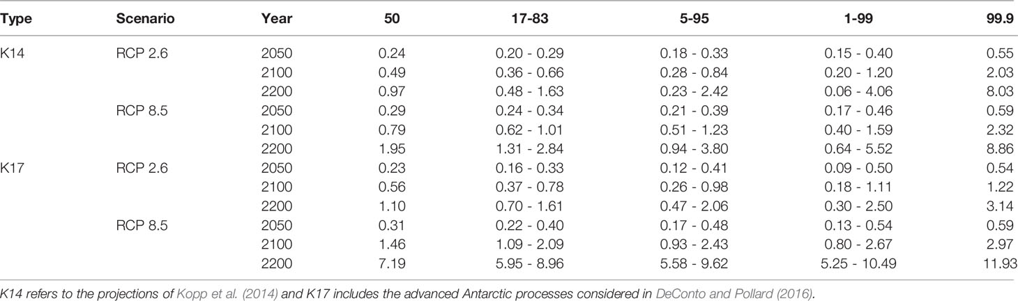
Table 1 Percentiles of projected sea-level rise (in meters) for the different RCP scenarios (from Kopp et al., 2017).

For our study, we created a method to generate the desired number of sea-level time series, over the period from 2000 to 2100 at a 1-year increment, from the percentiles given in the Table 1 from Kopp et al. (2017). To create these sea-level time series, which we refer to as pseudo-realizations, we fit a theoretical cumulative distribution to the provided percentiles in the provided years. Calculating the derivative of these theoretical cumulative distributions provides us with the probability density function. We sample the probability density function in each provided year using the Kernel Density Estimates method. We create an array with the size of the number of pseudo-realization for the year 2000 in which the sea level is defined as zero. Taking the sampled distributions in the years 2050, 2100, and 2200, we append values to the pseudo-realizations array for the provided years by randomly choosing a value from the sampled distribution in 2050, 2100, and 2200, respectively, for which η_sl(t_i+1) = η_sl(t_i) + Δ_i+1η_sl where t_i = 2050,2100,2200, and Δ_iη_sl is small range of sea level. As the last step, for each of the time series containing now values for 2000, 2050, 2100, and 2200, we employ polynomial function to interpolate for the years in the between t_i.

If the number of pseudo realizations is sufficiently large (>1000), the recalculated percentiles from the pseudo realizations fall within an error of less than 2% of the percentiles provided in Kopp et al. (2017).

2.2 Coastal Bathymetry Under Climate Change

From a modeling viewpoint, the influence of sea-level rise and other climate-change impacts on the nearshore bathymetry and, subsequently, the tsunami hazard can be incorporated in two different ways. The first way is to raise or lower the water level or mean sea level according to RCP sea-level projections, which is an approach that is also referred to here as the bathtub approach. As mentioned above, we consider this simple adjustment as static because features, such as barrier islands or marshes, do not change their horizontal locations. In the bathtub approach, adjustments due to sea-level rise only occur vertically, where the vertical adjustment is simplified to a one-to-one shift with sea-level rise.

The second approach to incorporating sea-level rise and climate-change impacts that alter bathymetries is to employ system-level simulation tools, such as the previously mentioned LTM model by Lorenzo-Trueba and Mariotti (2017). The LTM model solves a set of ordinary differential equations (ODEs) that calculate the horizontal and vertical positions of the subcomponents boundaries of the BML system. Figure 1 depicts the subcomponents of the LTM model. The red crosses show the locations of the governing equations, while the green arrows indicate important fluxes and parameters, but also where non-linear connections between the different equations exist. The red arrows mark the location of the important parameters, and important parameters, such as the barrier height (H_b) and width (W_b), or mainland-marsh width (W_bm).

FIGURE 1

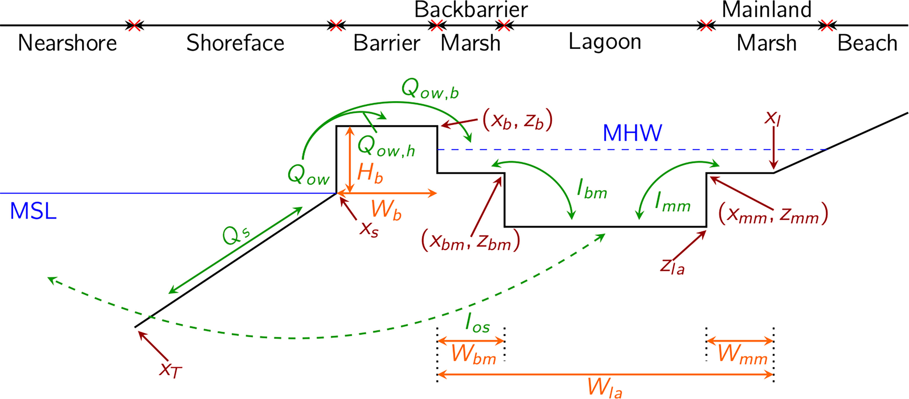
Figure 1 Setup for the Lorenzo-Trueba-Mariotti model with the simplified geometry of the BLM system. The red crosses mark the locations for the governing equations with the names of some of the variables in red. Important fluxes are given in green, while important measures, such as the barrier width and height (for example) are depicted in orange. Modified after Lorenzo-Trueba and Mariotti (2017).

Without loss of generality, the LTM model is a morphokinetic flux model, and, therefore, it does not focus on the physical, chemical, and biological processes directly to drive the development of the BML system. We refer to Lorenzo Trueba and Mariotti (2017, and references therein) for an extensive discussion about the governing equations and their inputs, initial conditions, and applications of the LTM model. As mentioned in the previous paragraph, the LTM model solves a set of coupled ODEs that describe the horizontal and vertical changes of the subcomponent boundaries (see Figure 1). The key parameters are listed in Table 2.

TABLE 2

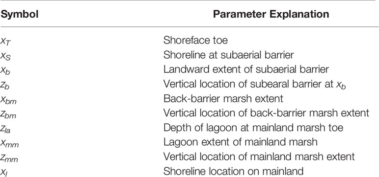
Table 2 Locations of subsystem boundaries simulated in the governing equations provided in Lorenzo-Trueba and Mariotti (2017).

Yet, this set of ODEs can be solved efficiently enabling us to create a Monte-Carlo-type computational framework.

The width of the barrier island is defined as W_b = x_b − x_s, the widths of the backbarrier (W_bm) and mainland (W_mm) marshes with W_bm = x_bm − x_b, and W_mm = x_l − x_mm. The lagoon width is calculated by W_la = x_l −x_b.

As mentioned earlier, climate change is the main driver of sea-level rise in the LTM model. However, other climate change impacts also affect the coastal and marine physical environment, for example, the nearshore wind speed or the sediment overwash flux (for more information about both parameters, see below) and can drive significant changes in the coastal system as a whole as well as its subsystems. To gain initial insights on which parameters are the most influential, we performed a small and limited sensitivity study, varying parameters found in Lorenzo Trueba and Mariotti (2017, Tables 1, 3). The result of this preliminary testing revealed that the shoreface sediment flux, Q_fs, the overwash sediment flux, Q_ow, and the influx of offshore sediment flux, I_os are the most sensitive processes and those that have the most significant impact on, the overall dynamics of the BML system. It is interesting to note that all three parameters (Q_fs, Q_ow, I_os) relate to climate change impacts in different ways. For example, wind speed predominantly controls the shoreface sediment flux. Eichelberger et al. (2008) and Zeng et al. (2019) study how climate change generally impacts wind speed. Tides and the concentration of nutrient-rich open-ocean sediment concentration govern the influx of nutrients into the lagoon and by fractionation the bounding marshes and impact I_os. Pickering et al. (2017) indicates that the impact of climate change on the tidal range and tidal wave period –both are a function of the shelf water depth– is at a maximum within 10% of today’s value. Therefore, the impact of future change in open-ocean sediment concentration is likely to have a much more significant impact on the influx of offshore sediments. Sediment overwash onto the barrier island and into marsh-lagoon subsystems is a necessary process. Leaving the ratio of overwash sediment flux that moves onto the barrier and into the marsh-lagoon subsystem constant, the magnitude of sediment overwash is the most significant parameter influencing the entire BML-system evolution, aside from sea-level change.

TABLE 3

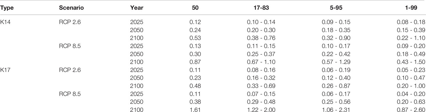
Table 3 Percentiles of projected sea-level rise (in meters) for the different RCP scenarios for 2025, 2050, and 2100, based on the pseudo-realization method.

The result of our aforementioned preliminary parameter study helps us to identify the parameters that need to be studied and put into the context of future climate change. Sea-level rise is, by far, the best-studied climate-change impact. However, open-ocean sediment concentration, overwash sediment flux, and wind speed as a function of climate change are not well understood, and future predictions are not available or part of ongoing controversial discussions within the respective scientific communities. To accommodate changing values for sediment overwash flux, wind speed, and open-ocean sediment concentration, we changed the original LTM model as presented by Lorenzo-Trueba and Mariotti (2017) slightly, without changing the governing equations. Furthermore, we also adopted the value ranges of sediment overwash sediment flux and the available offshore sediment from Lorenzo-Trueba and Mariotti (2017) and wind speeds from Zeng et al. (2019).

To account for future changes and trends of the open-ocean sediment concentration, wind speed, and overwash sediment flux, we assumed that the mean values of all three parameters over the period from 2000 to 2100 could either remain constant, increase or decrease. Again, ranges for end values for these different trends are taken from Lorenzo-Trueba and Mariotti (2017) and Zeng et al. (2019). Furthermore, we sample a Gaussian distribution of wind speed, overwash sediment flux, and available offshore sediment whose mean values are provided following the trend schemes mentioned above and standard deviations defined to be 10% of the respective mean value to create an, albeit, artificial spread of values in each year. We argue that this proposed method to mimic annual fluctuations simulates their stochastic nature as a Wiener process reasonably well.

Lastly, the geometry, especially of the barrier island, shown in Figure 1, is simplified, and the barrier does not feature a characteristic profile containing a dune. The barrier height as considered in the LTM model can be interpreted as an average height. Nevertheless, one could argue a profile containing a dune might have a significant influence on how a tsunami wave would overtop the barrier. Therefore, we assume that the dune is eroded by the tsunami wavefront as it travels over the island. Hence, we argue that the average barrier height is appropriate to describe the height of a barrier.

2.3 GeoClaw

We employ GeoClaw, part of Clawpack, for tsunami simulations (no sediment transport). GeoClaw has been under development since 1994 (i.e., George, 2008; Berger et al., 2011; LeVeque et al., 2011). Clawpack solves hyperbolic systems of partial differential equations in one, two, and three dimensions. For flow problems in large spatial domains, depth-averaged Shallow-Water equations (SWE) are usually sufficient. However, some problems appear in solving the SWE, especially for extreme wave propagation and flow over variable bathymetries and topographies. For this reason, a special subset of Clawpack, GeoClaw, includes adaptive mesh refinement (AMR) (Berger et al., 2011). GeoClaw has been employed for a variety of problems in tsunami science (e.g., MacInnes et al., 2013; Melgar and Bock, 2015; Melgar et al., 2016). GeoClaw is verified and validated with all problems given in NOAA’s standards and procedures for tsunami inundation codes (George, 2008), with a recent application and benchmarking for storm surges (Mandli and Dawson, 2014).

2.4 Earthquakes

We consider the earthquakes in this study to range from magnitudes M_w8.0 to M_w9.0 with 11 magnitude steps. We base the surface deformation field computations on random depth underneath the ocean floor between 5 km and 100 km while leaving the rake, dip, and strike angles constant. A total of 50 earthquakes in each magnitude step is used to ensure a stable tsunami-runup distribution. The area of the earthquake is computed using a standard empirical formula by Strasser et al. (2010). The earthquakes distance to the barrier island is kept constant at about 1970 km to ensure that the coastal environment is located in the far-field for any given earthquake.

2.5 Computational Domain and Parameter Study

As mentioned in the previous paragraph, the earthquake location is about 1970 km away from the BML system. The water depth is constant at 1000 m up to 1800 km from the earthquake area and then increases with a simple sloping beach where the shoreface in front of the barrier connects to the BML system. Figure 1 depicts the general BML system, while Figure 3 in Results below shows the BML system at scale (solid red line and a and b).

The barrier initially is 2 m high and 300 m wide, the back-barrier marsh is 4 km wide, the lagoon is 30 km long, and the mainland marsh initially is 2.5 km wide. These values do not represent any particular BML system by any means and are adopted from Lorenzo-Trueba and Mariotti (2017).

As discussed earlier, wind speed, overwash sediment flux, and open-ocean sediment concentration have profound impacts on the BML model, and, unlike sea-level rise, it is unclear how future changes under different RCPs influence the trends for these parameters. The table in Figure 6 contains the different assumed climate-change scenarios for these additional parameters and notes if the parameters remain constant, increase or decrease as described above. We acknowledge that many more combinations of constant, increasing and decreasing trends are possible among the three parameters, but argue that any additional combination can be realized by combining scenarios A-G with each other.

The parameter space of our study consists of the number of different RCP scenarios, two different treatments of Antarctic Ice Sheet uncertainty, the number of climate-change scenarios for additional parameters (wind speed, overwash flux, and sediment concentration), the number of realizations of the coastal-evolution model, the number of different earthquake magnitudes, and the number of different random depths for each earthquake magnitude. This results in a total of 2 RCPs (RCP 2.6 and 8.5) × 2 AIS models (K14 and K17) × 7 different climate-change scenarios (A-G) × 1000 (realizations per scenario) × 11 earthquake magnitudes × 100 earthquake depth per magnitude step, which totals 30,800,000 individual GeoClaw simulations on a modern Intel i7 (5th generation) processor, each GeoClaw simulation takes 4 minutes, which would result in a total computation time of 85 years. We, thus, make use of high-performance computing resources to execute these simulations.

3 Results

3.1 Sea-Level Rise Realizations

The range between the 5^thand 95^th percentile of the sea-level distribution as a function years is depicted in Figure 2, while Table 3 contains the median (50^th percentile), the percentile range 1-99, 5-95, and 17-83. From Figure 2A, we see that for RCP 2.6 the range between the 5^th (dotted lines) and the 95^th (dashed lines) percentiles is increasing to similar values through the years. We note that K14 between 2100 and 2120 is slightly larger than K17. In 2100, the 5^th- 95^th percentile range is between 0.45 m to 1.00 m for RCP 2.6. There are more significant differences between K14 and K17 for RCP 8.5 (Figure 2). Around the year 2030, the 5^th-95^th percentile ranges diverge, resulting in a range between 0.43 m and 1.5m for K14 and between 1.06 m and 2.6 m for K17 in 2100.

FIGURE 2

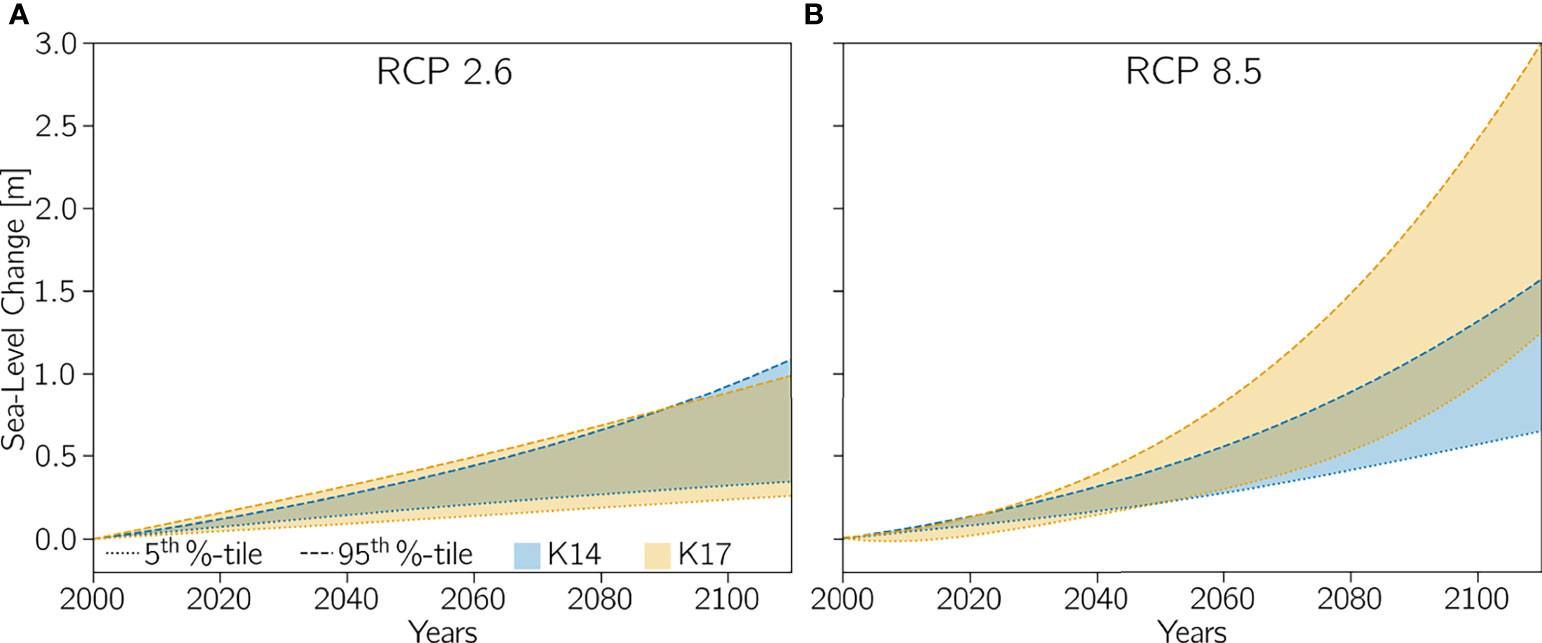
Figure 2 Pseudo realizations of sea-level change times series for (A) RCP 2.6, and (B) RCP 8.5.

From Table 3, we can see that the median values for RCP 2.6 K14 and RCP 8.5 K14 are similar for the years 2025 (RCP 2.6: 0.12 m; RCP 8.5: 0.13 m) and 2050 (RCP 2.6: 0.24 m; RCP 8.5: 0.30 m), but are significantly different for 2100 with 0.53 m for RCP 2.6 and 0.87 m for RCP 8.5. The median values for RCP 2.6 K17 and RCP 8.5 K17 for the year 2025 are the same, 0.11 m. In the year 2050 the values are 0.23 m for RCP 2.7 and 0.38 m for RCP 8.5. However a stark difference is apparent for the 2100 where the value for RCP 2.6 is 0.48 m and the value for RCP 8.5 is 1.61 m. Looking at the extreme values (95^th, 99^th, and 99.9^th percentiles), we see similar trends between RCP 2.6 and 8.5 for K14 and K17 as described for the median values.

3.2 Temporal Evolution of Static and Dynamic Bathymetric Models

Figure 3 depicts a comparison between the static (3a+c) and dynamic (3b+d) bathymetry models under sea-level rise. Both models are based on the same sea-level change time series and start with the same bathymetry (solid blue line). The simulations end at t_e = 100 years, which is indicated by the dashed blue line in both models.

FIGURE 3

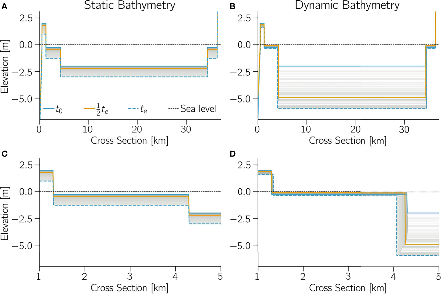
Figure 3 Example realization of simulated bathymetry, where bathymetry is either static (A, C) or dynamic (B, D); open ocean is to left. Note that the ower panes (C, D) show close-ups of back-barrier marsh and t_o is start of simulation (year 2000) while t_eis end of simulation (year 2100).

Comparing the end states of the static and dynamic model with each other, we can see that the barrier height in the static case significantly decreases, while the barrier height in the dynamic case changed very little from the year 2000 to 2100 (Figures 3B, D). Due to the simple dependence of the static model to sea-level change, the water layer over the marshes and the lagoon increases in thickness at the same rate, and the barrier decreases its height. The depth of the marshes in the dynamic model changed some, but it seems as if the marshes were able to maintain more or less the same depth as the sea level was rising, but marsh edge erosion reduced the marsh width. Furthermore, the lagoon depth at t_e is 6m in the dynamic model, significantly deeper than in the static model (lagoon depth at t_e = 3.7m). This result in itself is interesting, but the more interesting part from a theoretical point of view is the seemingly very non-linear response to the sea-level driving change in the early years of the simulation. The yellow lines mark the half time of the simulation $(\frac{1}{2}{t}_e=50years)$, and in the static model, the position of this yellow line is closer to the start state at time t_o (the year 2000) because the sea-level change solely governs the temporal development. It is projected that the sea level changes faster in the latter half of this century (> 50years) compared to earlier in this century. However, in the dynamic model, the yellow line is closer to the end at t_e, which indicates a very non-linear response of the lagoon depth to the relatively smaller sea-level change in the early years of the simulation. The lagoon depth for $\frac{1}{2}{t}_e<t<t_e$ does not change much.

3.3 Tsunami Run-Up

We employ the tsunami run-up as an indicator of the tsunami hazard, which is defined in our context as the vertical distance between the elevation of the maximum tsunami inundation and sea level. Tsunami run-up probability densities for all of the considered scenarios are provided in Figure 4 (RCP 2.6) and 5 (RCP 8.5). For both figures, the left column (a, c, and e) contains the static bathymetry results, and the right column (b, d, and f) the results for the dynamic bathymetry. Furthermore, the solid lines represented the run-up probability density for K14 and the dashed lines for K17; the different colors represent different years (orange: 2025, green: 2050, and blue: 2100).

FIGURE 4

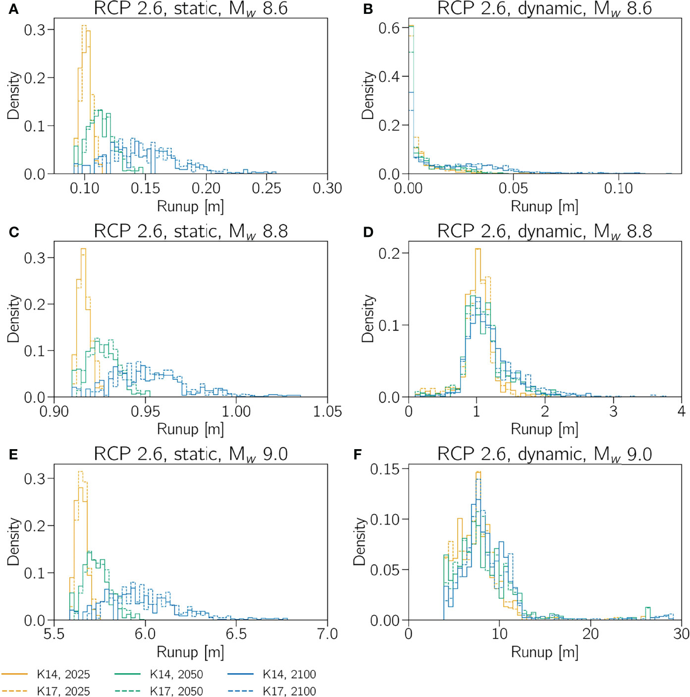
Figure 4 Probability densities of run-up for M_w8.6, 8.8, and 9.0 for RCP 2.6 for the static bathymetry (A, C, E) and dynamic bathymetry (B, D, F) for K14 and K17 for the years 2025, 2050, and 2100. Note that the ranges of the x-axes were chose to highlight the nearly order of magnitude differences between (A, C, E), and (B, D, F).

Focusing first on RCP 2.6 (Figure 4), we can see that the general geometry of the run-up probability density in the case of a static bathymetry (a, c, and e) for earthquake magnitudes 8.6, 8.8, and 9.0 are very similar, but note that the run-up values along the x-axes change significantly from values between 0.075 m and 0.28 m for M_w8.6, from 0.91 m - 1.04 m for M_w 8.8, and 5.52 m - 6.8 m for M_w 9.0. The changes from 2025 to 2100 are consistent with sea-level changes (see Table 3), which is the only variable for static bathymetry. Furthermore, note how the modes of the run-up densities move toward larger run-up values, and are more broadly distributed across run-up values, with increasing time. For the dynamic case (Figures 4B, D, F), the value ranges for the run-up probability densities show a similar increase for the three different earthquakes, which is close to an order of magnitude increase in run-up range from M_w 8.6 to M_w 8.8 to M_w 9.0. For M_w 8.8 and 9.0 scenarios, the probability densities for the dynamic case are skewed toward larger values, and the range of the K14 and K17 curves in a given year have a much wider spread compared to the static bathymetry. For example, the run-up density for K17 in the static bathymetry of M_w 8.8 in 2100 ranges from 0.91 m to 1.04 m, while the run-up density interval for the dynamic bathymetry for the same case reaches from 0.2 m to 3.8 m, exceeding the range of sea-level change in the same year significantly. Furthermore, the modes of the run-up probability density in the dynamic case for all years and AIS treatments (K14 and K17) are consistent for the three earthquake magnitudes; with the exception of a slight spreading toward higher run-up values with time, the density shape does not change in the different years.

For RCP 8.5 (Figure 5), observations about the run-up probability densities for the static and dynamic bathymetry and different earthquakes are similar to that for RCP 2.6. The ranges of run-up values for the static case are consistent with the sea-level rise ranges in the different years (see Table 3).

FIGURE 5

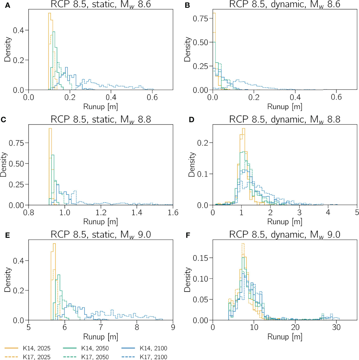
Figure 5 Probability densities of run-up for M_w8.6, 8.8, and 9.0 for RCP 8.5 for the static bathymetry (A, C, E) and dynamic bathymetry (B, D, F) for K14 and K17 for the years 2025, 2050, and 2100. Note that the ranges of the x-axes were chose to highlight the nearly order of magnitude differences between (A, C, E), and (B, D, F).

While the run-up probability densities for the static bathymetry (Figures 5A, C, F, and Figures 4A, C, F) are only a function of sea-level rise, the dynamic bathymetry evolution in time additionally depends on offshore sediment availability, overwash sediment flux, and wind speed. Figure 6 depicts the run-up values for an M_w 8.9 earthquake for RCP 2.6 and 8.5 for K14 and K17 as box plots. As a reminder, the line within the box marks the median run-up value, while the height of the box is referred to as the interquartile range (25^th- 75^th percentiles). We employ the 5^th percentile to define the location of the lower whisker and the 95^th percentile to defined the location of the upper whisker. Note that we exclude the date that is either below the 5^th and above the 95^th percentile as outlier values. The letters refer to the climate change scenarios as provided in the table included in Figure 6. Focusing on RCP 2.6 first (Figures 6A, B), we can see that the median run-up values of the different climate-change impact scenarios vary between 2.00 m and 3.75 for 2025, between 2.00 m and 4.64 m for 2050, and between 2.30 m and 4.10 m for 2100. Note that scenario E defines the maximum of provided intervals and scenario D the minimum for RCP 2.6 for K14 and K17. Interestingly, the median run-up values for scenario E are larger for K14 than for K17 in 2025 and 2050, while K17 is larger in the year 2100. For the interquartile range, the behavior in 2025 and 2050 is very similar. The interquartile range in 2025 has its minimum range at 0.17 m (scenario D) and its maximum at 1.76 m (scenario E, K14). For the year 2050, the maximum interquartile range is 2.30 m (scenario E, K17) and the minimum is 0.25 m (scenario D, K14). The previously described pattern of minimum and maximum interquartile ranges does not continue in the year 2100. In 2100, the maximum interquartile range for K14 is at 2.10 m with scenario E; the maximum for K17 occurs at scenario F with 1.86 m. The lower and upper whiskers exhibit a similarly consistent pattern for both K14 and K17. The largest upper whiskers occur in scenario E and increase from 2025 to 2100 is similar ways. However, the upper whisker for scenario E is with 6.36 m for K17 larger than the 6.09 m for K14, which is consistent with the slightly larger sea-level range as depicted in Figure 2. For the lower whiskers, it is interesting to observe that the minimum values occurs at scenario F and is close to zero for K14 for the years 2025, 2050, and 2100; while for K17 the minimum value is only close to zero in the years 2025 and 2050.

FIGURE 6

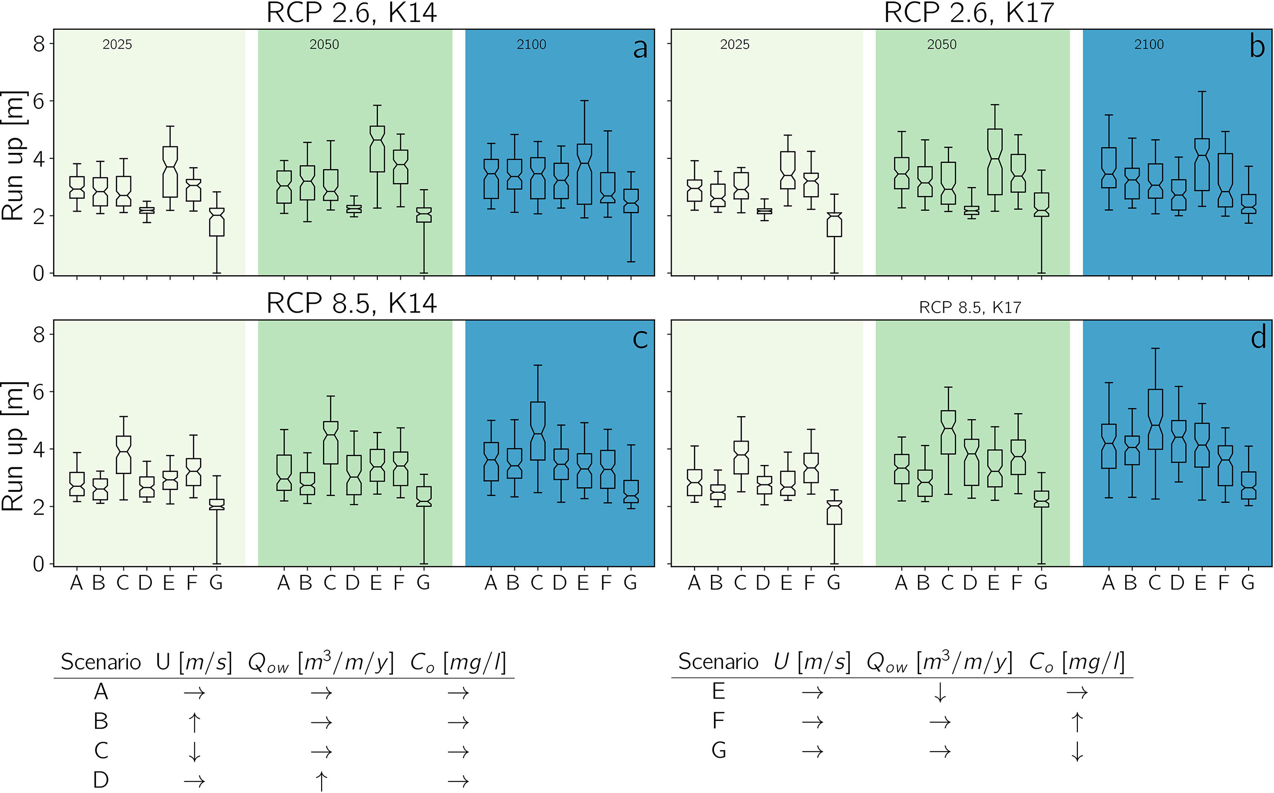
Figure 6 Run-up distributions for the different climate change scenarios for a M_w8.9 for RCP 2.6 K14 (A) and K17 (B), and RCP 8.5 K14 (C) and K17 (D). The different climate-change scenarios are of combinations of wind speed (U), overwash sediment flux (Q_ow), and sediment concentration in the open ocean (C_o) are given below. The range for ↑ (increasing) and ↓ (decreasing) varies between 5 – 15m/s for wind speed, 5 – 300m³/m/y for overwash sediment flux and 0.001 – 0.3mg/l for the open ocean sediment concentration The values for → are U = 10m/s, Q_OW = 100m³/m/y, and C_O = 0.1mg/l.

Figures 6C, D depict the run-up values as box plots for the different climate change scenarios and years for RCP 8.5. While for RCP 2.6, the maximum of the medians can be found at scenario E, the maximum median values occur at scenario C for RCP 8.5 for K14 and K17 (2025: 3.91 m [K14], 2050: 4.72 m [K17], and 2100: 4.85 m [K17]). The interquartile-range and whisker pattern are consistent between K14 and K17 from 2025 to 2100.

Figure 7 depicts the run-up as function of the earthquake magnitude for RCP 2.6 (a & b) and RCP 8.5 (c & d). The run-up values for RCP 2.6 for earthquake magnitude smaller than 8.8 (Figure 7A) are small with neither the median nor the maximum exceeding one meter in any given year. For larger earthquakes, the run-up values change dramatically for larger earthquakes (M_w 8.8 - M_w 9.0, Figure 7B) where the medians increase from about 1 m for M_w 8.8 to values between 3.5 m and 4.1 m for M_w 8.9 to values between 7.0 m and 8.3 m for M_w 9.0. Notably, while the median is highest for 2100, the maximum values of the tsunami run-up for K14 and K17 for a M_w 9.0 earthquake occurs in the year 2050 (Figure 7B). Similarly, the median and maximum values of tsunami run-up remain below one meter for M_w 8.5 to M_w 8.7 for RCP 8.5 (Figure 7C), except for K17 in 2100 whose maximum is 1.1 m. Furthermore, the median changes for larger magnitudes (Figure 7D), where median values have similar values compared to RCP 2.6. It should be noted here that the median values for K17 in the year 2100 for a M_w 9.0 earthquake is slightly larger. The biggest difference in run-up values for M_w between K14 and K17 for RCP 8.5 occurs in 2100. The maximum for RCP 8.5 K14 is 15 m, while the maximum for RCP 8.5 K17 with 30 m twice as large.

FIGURE 7

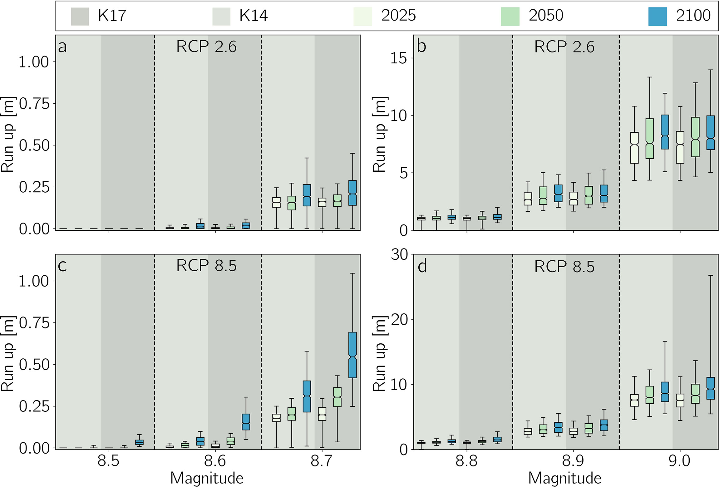
Figure 7 Comparison between run-up as a function of tsunami-genic earthquake magnitude and between RCP 2.6 for both K14 (A) and KP 16 (B) and the RCP 8.5, likewise for K14 (C) and K17 (D). The green-blue colors represent the years 2025, 2050, and 2100, while light and gray backgrounds respectively represent K14 and K17. The colored boxes represent the 17-83 percentile range, while the line within the box denotes the medians. The lower and upper whiskers mark the 5 - 95 percentile range.

4 Discussion

The comparison of Figures 3A, C with Figures 3B, D reveals that the static bathymetry responds linearly, meaning that sea-level rise changes the vertical location of the subsystems in the same way; there is neither a vertical nor a horizontal response of any of the BML subsystems to sea-level rise. On the other hand, the dynamic bathymetry, simulated with the LTM model by Lorenzo-Trueba and Mariotti (2017), shows how nonlinear the response is to sea-level rise, but also other climate change impacts, such as barrier-island sediment overwash flux (Q_ow in Figure 1). Not only is the evolution of the barrier-island-marsh lagoon-marsh system governed by a multitude of climate change impacts, of which only four were varied in this study, but individual subsystems also responded in a different way to the different drivers. For example, the barrier-island height changed very little. The back-barrier marsh kept up with the sea-level rise and exhibited edge erosion in the realization shown in Figure 3D (between 1.2- 4.3 km). However, the lagoon responded dramatically by deepening significantly early on. It should be noted that from our results it is impossible to conclude equilibrium conditions for each of the subcomponents. We refer to Lorenzo-Trueba and Mariotti (2017) for more discussion about equilibrium conditions for the BML system components.

Figures 4, 5 show how fundamentally different the impact of the static and dynamic bathymetry is on tsunami run-up. The modes of the run-up probability densities for the static bathymetry increase and spread over a wider range of values as the barrier islands height lowers with increasing sea level. In the dynamic case, however, the modes (maximums) of the run-up densities remain similar for the years, 2025, 2050, and 2100, which indicates that the barrier height does decrease significantly. Notably, for larger earthquakes the run-up modes for the static and dynamic bathymetries differ dramatically, with the dynamic being much larger; for M_w 9.0 the dynamic modes are 30 to 40% larger than the static modes (Figures 4, 5). Comparing the maximum values of run-up between the static and dynamic bathymetries with each other, it appears that the maximum values of run-up for the dynamic bathymetry are about three times larger than those of the static bathymetry. For the static bathymetry, sea-level rise controls bathymetric change and thus run-up. However, not surprisingly, in case of the dynamic bathymetry the barrier island alone does not govern the tsunami run-up. Other components of the system significantly impact the tsunami interaction with the BML system. Assuming that the tsunami run-up (ℜ) is propostional to the flow speed (u) we use the Froude number to find out that the run-up is propotional to the water depth:$\Re \propto \sqrt{d}$. The thickness of the water layer over lagoon increases dramatically in the dynamic bathymetry case but varies by only the sea level rise amount in the static bathymetry case (for example, see Figure 3). Hence, the lagoon’s water depth, which is generally deeper in the dynamic bathymetry case, governs the tsunami run-up and, therefore, the tsunami hazard.

It seems from Figure 7 that within one RCP scenario the pattern of medians, interquartile ranges and maximum and minimum values in the depicted box plots are consistent for the different magnitudes. This consistency increases our confidence in the results, especially in the LTM model because of its nature, simulating specific cases is a nontrivial endeavor. We employ the range of maximum and minimum values from the box plots in Figure 7 and the run-up probability densities for the dynamic case shown in Figures 4B, D, F, and 5B, D, F compared to the relative narrow peak of the run-up densities in Figures 4A, C E, and 5A, C, E for the static bathymetry as evidence that the nonlinear system response to other climate change impacts significantly affects the tsunami run-up distribution and, therefore, the tsunami hazards, but concede at the same time that sea-level rise carries the leading-order influence.

How climate change impacts other than sea-level rise (see table in Figure 6) affect the tsunami run-up distributions (Figure 6) is variable for different earthquakes and also changes from 2025 to 2100. Therefore, we argue that climate change impacts have nonlinear effects, but warn to not over-interpret the results herein and draw any conclusions on the relative importance of these additional climate-change parameters as listed in table included in Figure 6, because of their simplistic nature. We rather suggest that there is a need to put the other climate-change impacts important for coastal systems on theoretical foundation that is as robust as that for sea-level projections.

5 Conclusions

We recognize from our simulations that future projections of the tsunami hazard for a barrier-island-marsh coastal system are more sensitive to the choice of whether the coastal bathymetry and topography are changed statically (bathtub) or dynamically (with the help pf the LTM model) than they are to the specific RCP scenario that drive sea-level change and other climate change impacts. While there are differences between the impacts of RCP 2.6 and RCP 8.5 with (K17) and without (K14) enhanced AIS treatment, for the tsunami hazard the median values of run-up are correlated to differences in sea-level rise as the leading-order influence on the evolution of the coastal system. Other climate-change impacts, such as wind and wave climate, have second-order influence, but help to skew the run-up probability densities to larger extremes. Because extreme values are important for planning and design, it is crucial to consider how the individual subsystems respond to the different climate-change impacts governing system evolution (see. Lorenzo-Trueba and Mariotti, 2017). Furthermore, more work is needed to study climate-change impacts on coastal systems, bringing in, for example, prediction of future conditions impacting biological processes, in par with the robustness of sea-level change projections. Most likely the integration of these additional processes will contribute to widening the run-up probability density function, but will ensure that the tsunami hazard is fully understood and that uncertainties more fully quantified.

Taking what we learned from our study directly, for example, how climate-change impacts can alter the coastal geomorphology (not “just” sea-level rise), we emphasize that any evaluation of the future tsunami hazard must incorporate future geomorphic changes of the underlying nearshore bathymetry and topography in a dynamic and realistic fashion. At a minimum, the location of the shoreline must be established relative to the tsunami run-up. In this regard, field-based geologic investigations of tsunami records in any given region add significant value to tsunami hazard assessments. Not only can such geologic investigations help to validate some of the underlying statistical assumptions of tsunami frequency in any given region, but such investigations also help to put the tsunami run-up in the past into the context of the conditions of the coastal system at the time of run-up and, thereby, may be used to validate coastal-change models, such as the LTM model. Lastly, we urge that integrated theoretical and field-based studies must also focus on the evolution of the coastal system, its nonlinear responses to climate change impacts in the past and future, and the uncertainties associated with the geologic record.

Data Availability Statement

The original contributions presented in the study are included in the article/supplementary material. Further inquiries can be directed to the corresponding author.

Author Contributions

RW created the concept and generated all the codes to couple models, analyzed the data and produced the figures. Furthermore, RW was responsible for writing. TD and JI contributed to the concept and with writing and editing the manuscript. All authors contributed to the article and approved the submitted version.

Funding

This material is based upon work supported in part by the National Science Foundation under Grants GLD-1630099 and DGE-1735139 and by the U.S. Army Corps of Engineers through the U.S. Coastal Research Program (under Grant No. W912HZ -20-2-0005.

Conflict of Interest

The authors declare that the research was conducted in the absence of any commercial or financial relationships that could be construed as a potential conflict of interest.

Publisher’s Note

All claims expressed in this article are solely those of the authors and do not necessarily represent those of their affiliated organizations, or those of the publisher, the editors and the reviewers. Any product that may be evaluated in this article, or claim that may be made by its manufacturer, is not guaranteed or endorsed by the publisher.

Acknowledgments

Data were not used, nor created for this research. JLI and RW would like to thank the University of Haifa and the Morris Kahn Marine Station (University of Haifa) for their hospitality during the sabbatical, and JLI thanks the U.S. Fulbright Program and the United States-Israel Educational Foundation for support during her stay.

References

Berger M. J., George D. L., LeVeque R. J., Mandli K. T. (2011). The GeoClaw Software for Depth-Averaged Flows With Adaptive Refinement. Adv. Water Resour. 34, 1195–1206. doi: 10.1016/j.advwatres.2011.02.016

CrossRef Full Text | Google Scholar

DeConto R. M., Pollard D. (2016). Contribution of Antarctica to Past and Future Sea-Level Rise. Nature 531, 591–597. doi: 10.1038/nature17145

PubMed Abstract | CrossRef Full Text | Google Scholar

Dura T., Garner A. J., Weiss R., Kopp R. E., Engelhart S. E., Witter R. C., et al. (2021). Changing Impacts of Alaska-Aleutian Subduction Zone Tsunamis in California Under Future Sea-Level Rise. Nat. Commun. 12, 7119. doi: 10.1038/s41467-021-27445-8

PubMed Abstract | CrossRef Full Text | Google Scholar

Eichelberger S., Mccaa J., Nijssen B., Wood A. (2008). Climate Change Effects on Wind Speed. NAm Wind 7, 68–72.

Google Scholar

George D. L. (2008). Augmented Riemann Solvers for the Shallow Water Equations Over Variable Topography With Steady States and Inundation. J. Comput. Phys. 227, 3089–3113. doi: 10.1016/j.jcp.2007.10.027

CrossRef Full Text | Google Scholar

Kopp R. E., DeConto R. M., Bader D. A., Hay C. C., Horton R. M., Kulp S., et al. (2017). Evolving Understanding of Antarctic Ice-Sheet Physics and Ambiguity in Probabilistic Sea-Level Projections. Earth’s Future 5, 1217–1233. doi: 10.1002/2017EF000663

CrossRef Full Text | Google Scholar

Kopp R. E., Horton R. M., Little C. M., Mitrovica J. X., Oppenheimer M., Rasmussen D. J., et al. (2014). Probabilistic 21st and 22nd Century Sea Level Projections at a Global Network of Tide Gauge Sites. Earth’s Future 2, 383–406. doi: 10.1002/2014EF000239

CrossRef Full Text | Google Scholar

LeVeque R. J., George D. L., Berger M. J. (2011). Tsunami Modelling With Adaptively Refined Finite Volume Methods. Acta Numerica 20, 211–289. doi: 10.1017/S0962492911000043

CrossRef Full Text | Google Scholar

Li L., Switzer A. D., Wang Y., Chan C. H., Qiu Q., Weiss R. (2018). A Modest 0.5-M Rise in Sea Level Will Double the Tsunami Hazard in Macau. Sci. Adv. 4. doi: 10.1126/sciadv.aat1180

CrossRef Full Text | Google Scholar

Lorenzo-Trueba J., Mariotti G. (2017). Chasing Boundaries and Cascade Effects in a Coupled Barrier-Marsh-Lagoon System. Geomorphology 290, 153–163. doi: 10.1016/j.geomorph.2017.04.019

CrossRef Full Text | Google Scholar

MacInnes B., Gusman A., LeVeque R., Tanioka Y. (2013). Comparison of Earthquake Source Models for the 2011 Tohoku Event Using Tsunami Simulations and Near-Field Observations. Bull. Seismol. Soc. America 103, 1256–1274. doi: 10.1785/0120120121

CrossRef Full Text | Google Scholar

Mandli K., Dawson C. (2014). Adaptive Mesh Refinement for Storm Surge. Ocean Modeling 75, 36–50. doi: 10.1016/j.ocemod.2014.01.002

CrossRef Full Text | Google Scholar

Melgar D., Allen R., Riquelme S., Geng J., Bravo F., Baez J., et al. (2016). Local Tsunami Warnings: Perspectives From Recent Large Events. Geophys. Res. Lett. 43, 1109–1117. doi: 10.1002/2015GL067100

CrossRef Full Text | Google Scholar

Melgar D., Bock Y. (2015). Kinematic Earthquake Source Inversion and Tsunami Run-Up Prediction With Regional Geophysical Data. J. Geophys. Res.: Solid Earth 120, 3324–3349. doi: 10.1002/2014JB011832

CrossRef Full Text | Google Scholar

Nagai R., Takabatake T., Esteban M., Ishii H., Shibayama T. (2020). Tsunami Risk Hazard in Tokyo Bay: The Challenge of Future Sea Level Rise. Int. J. Disaster Risk Reduction 45, 101321. doi: 10.1016/j.ijdrr.2019.101321

CrossRef Full Text | Google Scholar

Pickering M., Horsburgh K., Blundell J., Hirschi J. M., Nicholls R., Verlaan M., et al. (2017). The Impact of Future Sea-Level Rise on the Global Tides. Cont. Shelf Res. 142, 50–68. doi: 10.1016/j.csr.2017.02.004

CrossRef Full Text | Google Scholar

Riahi K., Rao S., Krey V., Cho C., Chirkov V., Fischer G., et al. (2011). Rcp 8.5—A Scenario of Comparatively High Greenhouse Gas Emissions. Climatic Change 109, 33–57. doi: 10.1007/s10584-011-0149-y

CrossRef Full Text | Google Scholar

Stocker T. F., Qin D., Plattner G. K., Tignor M., Allen S. K., Boschung J., et al. (2013). “Climate Change 2013: The Physical Science Basis,” in Working Group I Contribution to the Fifth Assessment Report of the Intergovernmental Panel on Climate Change. (Cambridge, United Kingdom and New York, NY, USA: Cambridge University Press), 1535 pp.

Google Scholar

Strasser F. O., Arango M. C., Bommer J. J. (2010). Scaling of the Source Dimensions of Interface and Intraslab Subduction-Zone Earthquakes With Moment Magnitude. Seismol. Res. Lett. 81, 941–950. doi: 10.1785/gssrl.81.6.941

CrossRef Full Text | Google Scholar

van Vuuren D., Edmonds J., Kainuma M., Riahi K., Thomson A., Hibbard K., et al. (2011). The Representative Concentration Pathways: An Overview. Climatic Change 109, 5–31. doi: 10.1007/s10584-011-0148-z

CrossRef Full Text | Google Scholar

Zeng Z., Ziegler A., Searchinger T., Yang L., Chen A., Ju K., et al. (2019). A Reversal in Global Terrestrial Stilling and Its Implications for Wind Energy Production. Nat. Climate Change 9, 979–985. doi: 10.1038/s41558-019-0622-6

CrossRef Full Text | Google Scholar