Earth Observation and Machine Learning Reveal the Dynamics of Productive Upwelling Regimes on the Agulhas Bank

1 Introduction

Machine Learning (ML) and satellite observation methods have the potential to address the unique challenges that ocean physical and biological interactions pose (e.g., Rolf et al., 2021), especially in complex oceanic regions. With global coverage and long-term biological and physical observations, satellite remote sensing is an effective technology for understanding ocean processes. Unsupervised ML is a major class of ML that can cluster and reveal significant patterns in high dimensional datasets such as satellite ocean observations (Arnault et al., 2021; Sonnewald et al., 2021). Unsupervised ML identifies relationships among satellite observations of environmental parameters and reduces their large dimensionality, while removing unstructured noise (Boukabara et al., 2021; Rolf et al., 2021; Sonnewald et al., 2021). Successful applications of unsupervised ML to satellite observations to understand complex ocean dynamics have been made in recent decades (Sonnewald et al., 2021). These techniques include k-means, Self-Organizing Maps (SOM), t-SNE, autoencoders and Generative Adversarial Networks (GAN) (Sonnewald et al., 2021). For example, the application of k-means, a space-partitioning algorithm, to satellite ocean colour data identified regions with distinct marine biological activity (Ardyna et al., 2017). The SOM, a neural network-based clustering algorithm, found several applications in extracting spatial and temporal characteristic ocean current patterns using satellite sea surface height, current and surface salinity data (e.g., Liu et al., 2016; Arnault et al., 2021). A GAN, a method that generates new samples with similar distributions as the learning dataset, was used to reconstruct sea surface heights of the North Sea (Zhang et al., 2020; Yu and Ma, 2021). Extensive reviews of the advances and opportunities associated with ML application to satellite Earth observations and ocean science are provided by Boukabara et al. (2021) and Sonnewald et al. (2021). Here, we use the SOM to study intermittent productive upwelling regimes on the Agulhas Bank.

The Agulhas region (South Africa, Figure 1), where waters from the Indian, Atlantic and Southern Ocean meet, is oceanographically complex and amongst the most complex flow regions of the global ocean (Rujitier et al., 2003; Jackson et al., 2012). Numerous biophysical structures, driven by both atmospheric and oceanographic forcing, occur here (Roberts, 2005; Goschen et al., 2015). Its dominant circulation feature is the Agulhas Current (AC) which affects and is influenced by the hydrography of the Agulhas Bank (Lutjeharms, 2006). The AC originates, in part, from eddies and rings flowing southward along the Mozambican coast and westward from the Southeast Madagascar Current (SEMC) (Lutjeharms, 2006; Figure 1). The AC follows the African continental shelf slope, which remains very narrow until Port Elizabeth (~34°S), except at KwaZulu Natal Bight (~30°S) where the shelf widens and a solitary meander called a Natal pulse can form (Harris et al., 1978; Lutjeharms, 2006; Jackson et al., 2012; Figure 1). Note that the Natal Pulse can displace the AC (up to 200 km offshore) from its usual position as it propagates downstream along the coast with the current (Gründlingh, 1979; Lutjeharms, 2006) and can lead to the shedding of Agulhas rings (van Leeuwen et al., 2000). The southern AC (south of ~34°S), which is more unstable due to horizontal shear instability (Paldor and Lutjeharms, 2009), meanders south-westward along the southeastern edge of the wider Agulhas Bank. It then retroflects eastward (usually at 18-20°E and 39.5°S) and becomes the Agulhas Return Current (ARC) (Russo et al., 2021; Figure 1). The retroflection results in the shedding of filaments and eddies (Blanke et al., 2009). Along the southwestward path of the southern AC, cyclonic eddies (shear edge eddies) form on the current’s landward edge (Lutjeharms et al., 2003; Figure 1).

FIGURE 1

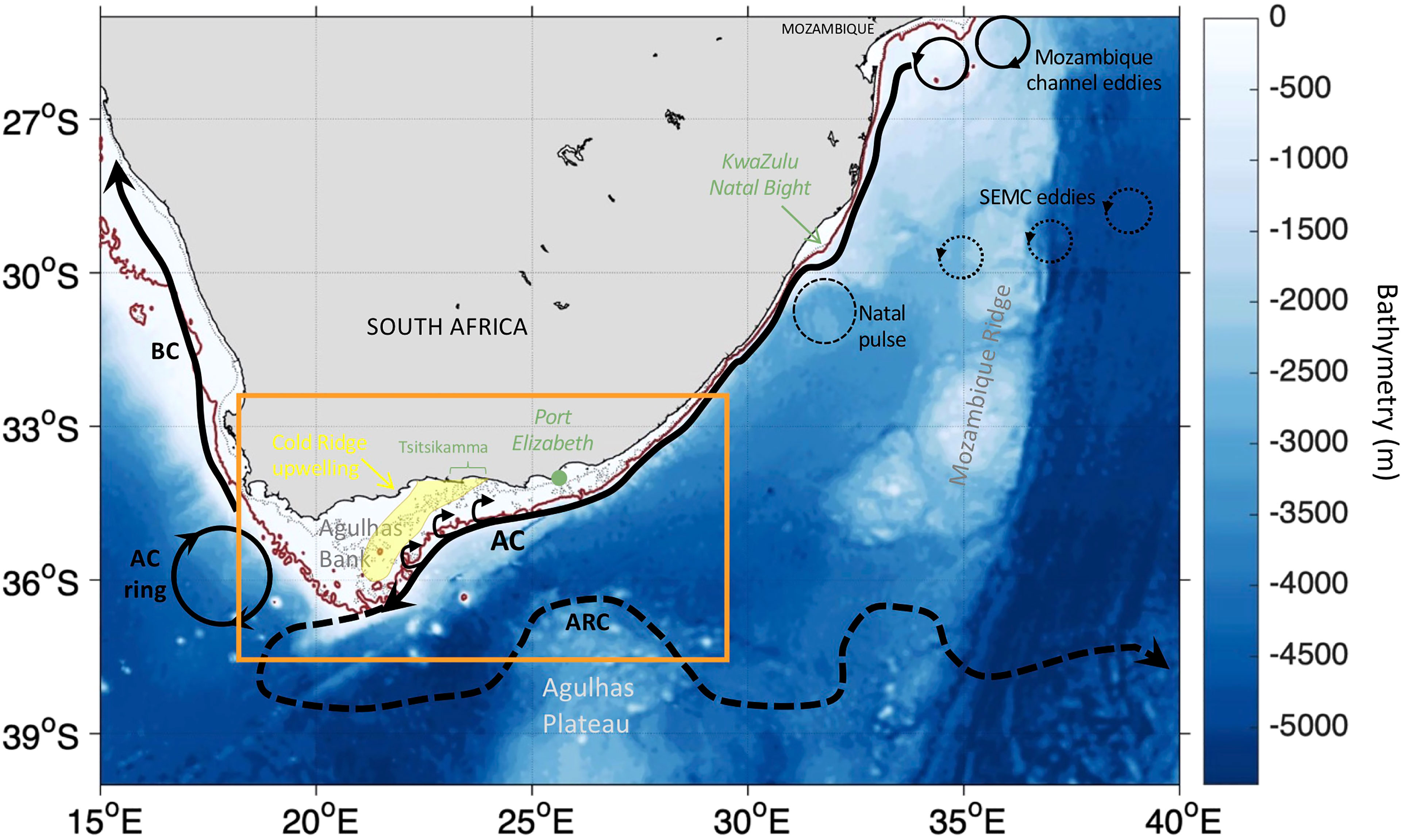
Figure 1 Bathymetry (in m), a schematic of the surface circulation over the Agulhas region based on Lutjeharms, (2006) and Russo et al., (2021) and the area of interest (orange box). The Agulhas Current (AC), the Agulhas Return Current (ARC) and the Benguela Current (BC) are illustrated with the thin black arrows. The thick black arrows along the southern AC at the shelf edge represent shear edge eddies. An AC ring is shown with a thick black circle. Eddies originating from the Mozambique channel and the Southeast Madagascar Current (SEMC) are designated by thin and dotted black circles, respectively. A Natal pulse is indicated with the thin dashed black circle. The approximate locations of the Cold Ridge upwelling is illustrated with a light yellow shaded area. The 100m and 200m isobaths derived from ETOPO2v1 global gridded database are represented by the dotted thin black and solid dark-red lines, respectively.

Due to its position, separating shelf waters from offshore waters, the AC plays a key role in regulating cross-shelf exchanges (Lutjeharms, 2006). The southern AC intensification and divergence from the coast generates shelf-edge upwelling (Blanke et al., 2009; Leber et al., 2017; Malan et al., 2018). The AC oceanic influence extends beyond the shelf edge (Lutjeharms, 2006), as AC water advects onto the eastern Agulhas Bank (Swart and Largier, 1987), due to southwesterly winds (Goschen and Schumann, 1990) or meanders (Lutjeharms et al., 2003), and from the eastern towards the western Bank (Jackson et al., 2012). AC’s Natal Pulse can contribute to upwelling in both the outer and inner shelf regions (Krug et al., 2014). Coastal wind-driven upwelling takes place over the coastal Bank during austral summer (November to March, Nov-Mar) when westward winds prevail (Schumann, 1999; Jackson et al., 2012). Wind-driven upwelling during the austral summer occurs also over the central Bank, along the 100m isobath, bringing cold, fresh, nutrient-rich (Lutjeharms et al., 1996) water to the surface (Boyd and Shillington, 1994; Probyn et al., 1994; Roberts, 2005). This cold filament is commonly called the “Cold Ridge” and extends from the Tsitsikamma coast in an offshore southwesterly direction (Roberts, 2005; Jackson et al., 2012). The Cold Ridge formation has also been linked to the westward transport hypothesis (where westward currents transport Chokka squid paralarvae from the eastern to the central Bank) (Roberts, 2005) and the westward advection of nutrients (Jacobs et al., 2022).

The seasonal Cold Ridge is important for the productivity over the Agulhas Bank (Jacobs et al., 2022), which impacts commercially valuable fisheries including hake, anchovy, sardine, horse mackerel, rock lobster and Chokka squid (Roberts, 2005; Brick and Hasson, 2016). Phytoplankton blooms and their phenology were found to be tightly linked to winds and squid catches in South Africa waters (Jebri et al., accepted). However, surface currents, which can impact paralarval movements (e.g., Lipiński et al., 2016) and upwelling, hence nutrients and phytoplankton productivity, are less well studied. Previous research that investigated interactions between the AC variability and the Bank and how they affect the productivity, or the larvae retention/loss, were largely based on limited in-situ data (e.g., Jackson et al., 2012 from a single cruise in Sep 2010) and Lagrangian particle tracking in models (e.g., Jacobs et al., under review), respectively. Other modelling and satellite observation studies examined mesoscale seasonal and interannual variability within the AC (Backenberg et al., 2012; Krug and Tourandre, 2012; Elipot and Beal, 2018), but only at localized parts of the Bank and not in relation to phytoplankton productivity. The complex interaction of the AC with the continental shelf waters is still not well understood. Questions about the AC’s different modes/topologies, their interannual variation and impact on the phytoplankton productivity over the Bank during the Cold Ridge upwelling season, remain unanswered.

Our objective, here, is to gain insight into the AC modes/topologies and circulation patterns which affect the Cold Ridge upwelling signature (in terms of phytoplankton biomass), and to study their interannual variations. To achieve this, we apply an unsupervised ML approach, the neural clustering Self Organizing Maps (SOM, Kohnen, 1982; Kohonen, 2014), to 23 years of satellite observations of surface currents, Sea Surface Temperature (SST) and chlorophyll-a (Chl-a, proxy for phytoplankton biomass and productivity). Note that although the Cold Ridge upwelling is triggered by south-westerly winds (Probyn et al., 1994; Roberts, 2005), here we only focus on the surface currents influence which enhances the upwelling productivity via westward advection (Jebri et al., 2022; Jacobs et al., submitted a). This multi-parameter SOM analysis is used to identify the most characteristic modes of the circulation that may lead to high and/or low productivity during the Cold Ridge season. The high variability of the AC and the lack of continuous and repeated in-situ observations, make satellite data and the SOM algorithm well suited to our study goal. The SOM algorithm (Kohnen, 1982), which has seen a wider application in recent years in ocean science (Liu and Weisberg, 2011; Arnault et al., 2021), has the advantage of higher discriminant power (distinguishing between the different clusters) and the ability to deal with the nonlinear aspects of the biophysical phenomena we aim to analyze, as compared to other ML (e.g., K-means; Badran et al., 2005) or statistical (e.g., the Empirical Orthogonal Functions [EOF]; Lorenz, 1956) methods (Jouini et al., 2016).

The paper is organized as follows: the datasets and the SOM methodology are presented in section 2. The SOM outputs are analysed to retrieve AC modes and their link to SST and Chl-a over the Cold Ridge path in sections 3.1 and 3.2. Interannual variations of the extracted currents, SST and Chl-a patterns are examined in section 3.3. In section 4, we discuss the currents and Chl-a patterns and their anomalous sequences in light of previous studies and climate variability modes’ extremes. Conclusions are given in section 5.

2 Material and Methods

2.1 Satellite Derived Data

Daily satellite-derived Chl-a concentrations (mg/m³), at a spatial resolution of 4 km, are developed by ACRI-ST based on the Copernicus-GlobColour processor (Gohin et al., 2002). This ocean colour dataset is a multi-satellite (SeaWiFS, MODIS, MERIS, VIIRS-SNPP & JPSS1, OLCI-S3A & S3B), global, reprocessed and cloud free product, downloaded from the Copernicus Marine Environment Monitoring Service (CMEMS) (http://marine.copernicus.eu/services-portfolio/access-to-products/). We use this Chl-a product over the time period 04 September 1997 to December 2020 to derive the Chl-a SOM patterns variability over a sub-domain in the Agulhas region which covers the Agulhas Bank and extends farther offshore to better encompass the AC variability (see Figure 1, orange box). Satellite-derived Chl-a observations may be overestimated in shallow waters (generally < 30m, Zhang et al., 2006). This is because suspended material and dissolved organic matter, which are present in these optically complex Case-II waters, can lead to high water leaving radiance and an overestimation of the correction term (IOCCG, 2000). However, high satellite Chl-a values in shallow areas are not necessarily erroneous, as they may represent chlorophyll-rich detritus from riverine inputs near the coast (Raitsos et al., 2013; Raitsos et al., 2017). Coastal elevated Chl-a values (>3 mg/m³) cover a very narrow band compared to the rest of the study area here which comprises mainly Case-I open ocean waters.

The multi-satellite (AVHRR, VIIRS, AMSR2, GOES13) global Met Office Operational-Sea-Surface-Temperature-and-Sea-Ice-Analysis (OSTIA, Good et al., 2020) SST product, acquired from CMEMS (http://marine.copernicus.eu/services-portfolio/access-to-products/) is used. This SST dataset is provided gap-free and daily at 5 km spatial resolution over the period 01 January 1981 to 31 June 2020 as a reprocessed version and from 01 July 2020 to present as a near-real-time version. Here, only the daily composites from 01 September 1997 to 31 December 2020 are considered, to match the satellite Chl-a dataset.

Finally, we utilize the altimetry derived SSALTO/DUACS absolute geostrophic currents (delayed time DT2018 version) processed and distributed by CMEMS (http://marine.copernicus.eu/services-portfolio/access-to-products/) (previously by AVISO (Archiving, Validation and Interpretation of Satellite Oceanographic Data)). This multi-satellite (Jason-3, Sentinel-3A & 3B, HY-2A, Saral/AltiKa, Cryosat-2, Jason-2, Jason-1, T/P, ENVISAT, GFO, ERS1/2) currents dataset consists of daily geostrophic zonal (U) and meridional (V) velocities gridded at 25 km spatial resolution from the delayed time version for the period 01 January 1993 to 03 June 2020 and from the near-real-time version for the period 04 June 2020 to present. We consider daily means from 01 September 1997 to 31 December 2020, to match the satellite Chl-a data in the SOM algorithm, in order to derive the regional surface circulation spatial patterns and variability modes. Satellite altimetry currents can be affected by sensor limitation near the coast (due to contamination of the sensor near land) (e.g., Cipollino et al., 2017). However, our study region comprises mostly open offshore waters. Additionally, the currents product version used here is characterized by a reduction in error on geostrophic currents estimation in coastal areas by more than 15% (Taburet and Pujol, 2022).

As the focus of this paper is on the seasonal behaviour of the Agulhas Bank upwelling, only data for the austral summer (November to March) each year are analysed in what follows. All satellite datasets (SST, Chl-a) were scaled up to the same spatial resolution of 25 km (the currents’ resolution) using a linear re-gridding. The high Chl-a data near the coast were masked out with the re-gridding (not shown), hence Chl-a was chosen over log10 transformation of Chl-a.

2.2 Unsupervised Learning: SOM

2.2.1 Concept and Architecture

The SOM is an effective method for extraction and clustering of spatial and temporal features (patterns) (Kohonen, 1982; Kohonen, 2001; Liu et al., 2006a; Liu et al., 2006b). The SOM retains the topology of the input datasets (i.e., conserves in the output the neighbour relationships between the inputs), even from noisy data, revealing correlations that are not easily identified with standard statistical methods such as Empirical Orthogonal Function (EOF) (Liu et al., 2006a). The SOM analysis has been applied in many fields (Kaski et al., 1998; Oja et al., 2003; Hong et al., 2004; Hong et al., 2005). In oceanography, it was found useful for the extraction and analysis of currents, wind, SST, Sea Surface Height and Sea Surface Salinity patterns (Richardson et al., 2003; Liu and Weisberg, 2005; Liu et al., 2006a; Mihanović et al., 2011; Jouini et al., 2016; Liu et al., 2016; Arnault et al., 2021).

The SOM is a competitive neural network based on unsupervised learning (Kohonen, 1982; Vesanto et al., 2000). It takes a high-dimensional input space and maps it onto a low dimensional grid, while conserving relationships between the inputs. The SOM is organized in two distinct layers (Kohonen, 1982; Vesanto et al., 2000) (e.g., Figure 2). The first (or input) layer takes a high-dimensional dataset to be clustered (called the input dataset). Here, the input dataset is composed of the satellite U and V, SST and Chl-a over the study region (see Figure 1, orange box and section 2.1). The second layer, which is the output layer, consists of a given number of nodes (neurons, units, clusters or patterns) topologically structured in a low-dimensional 2D grid (map) (Kohonen, 1982; Vesanto et al., 2000; Jouini et al., 2016). The number of output neurons is user-defined following the level of detail and degree of accuracy required in the analysis (Richardson et al., 2003; Jouini et al., 2016). Each neuron in the output layer has a weight vector connected to a subset of the input dataset and to its neighbouring neurons by a neighbourhood function, which dictates the map topology (Vesanto et al., 2000; Richardson et al., 2003; Jouini et al., 2016; Liu et al., 2016). Indeed, the SOM’ neurons are connected in way that determines a topological (neighbourhood) relationship between them (Jouini et al., 2016). Close neurons correspond to similar weight vectors, while distant neurons relate to different weight vectors (Jouini et al., 2016).

FIGURE 2

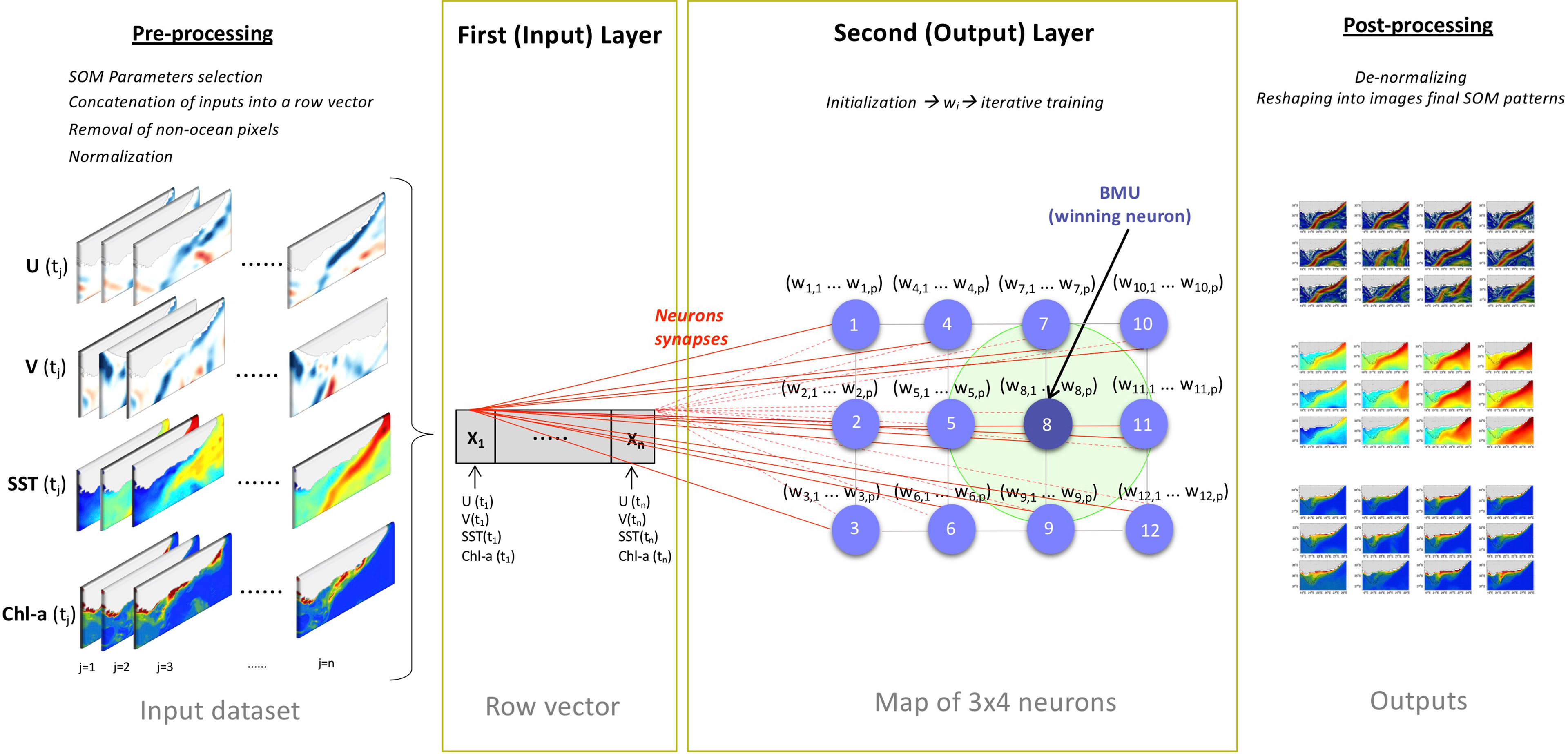
Figure 2 Summary diagram of the 3x4 SOM architecture and functioning described in section 2.2. During the pre-processing, the input dataset which consist of 2-D daily satellite data (U(tj), V(t_j), SST (t_j), Chl-a(t_j) with j=1: n days) is concatenated into a row vector X (which makes up the input layer). X is composed of n=3479 arrays (one for each day of the observational record) each of p=4416 elements (1104 pixels *4 variables). Each SOM neuron (or pattern) gets assigned a weight vector ((w_1,1… w_1,p)… (w_12,1… w_12,p)) that changes with the iterative training (second layer). When a BMU (wining neuron, dark blue circle) is found its weight vector and neighbouring neurons (light green shaded area) are updated. During the post-processing, the SOM outputs are reshaped into 2-D images.

The SOM algorithm organizes the grid (map) by first comparing the input data to each neuron (Liu et al., 2006a). The neuron which best matches the input vector (i.e., with the smallest Euclidean distance) is the winner neuron (or Best Matching Unit, BMU) and the centre of neighbouring neurons (Richardson et al., 2003; Liu et al., 2016; Liu et al., 2006b). The SOM, then, updates the excited neighbouring neurons and their associated weights (Richardson et al., 2003). This iterative training process is called self-organizing (Liu et al., 2016). There are two types of self-organizing: a traditional sequential training and a batch training (Liu et al., 2006a). The sequential training provides the input samples successively to the SOM, while gradually adjusting the weight vectors. In the batch training, the SOM receives the whole input dataset at once and the final weight vectors become the weighted averages of the data vectors associated with each node (Liu et al., 2006a). After the self-organizing process converges, the output weight vectors characterize the dominant patterns from the input data (Liu et al., 2016). Figure 2 sums up the architecture and functioning of the SOM algorithm described above. Here, we use the batch training approach (cf. section 2.2.2).

We use the MATLAB SOM-Toolbox version 2.0 (Vesanto et al., 2000; Kohonen, 2014), which is an efficient SOM implementation developed by the Laboratory of Information and Computer Science in the Helsinki University of Technology freely available at http://www.cis.hut.fi/projects/somtoolbox/. This toolbox was successfully used previously in oceanographic applications (Jouini et al., 2016; Liu et al., 2016; Liu et al., 2006a; Liu et al., 2006b; Arnault et al., 2021). The mapping quality of the SOM can be quantified through the average quantization error (QE) and topographic error (TE) which are returned by the toolbox (Liu et al., 2006a). QE indicates the average distance between data vectors and the BMU, while TE represents the data vectors’ percentage where the first and second BMU are not neighbouring neurons (Liu et al., 2006a). In other words, QE measures how accurate is the representation of the input data while TE measures the topology preservation (Hernandez-carrasco and Orfila, 2018; Meza‐Padilla et al., 2019). The lower QE and TE, the better is the mapping quality (Liu et al., 2006a). However, QE and TE decrease with increasing and decreasing map sizes, respectively, leading to a careful trade-off between mapping accuracy and preservation of the topology (Mihanović et al., 2011; Meza‐Padilla et al., 2019). The SOM-Toolbox returns also the BMU timeseries using the function som_bmus, which allows the identification of how the dominant neurons (patterns) vary/occur over time. More details about the implementation of the SOM using the toolbox are available in Kohonen (2014).

2.2.2 Parameterization

The parametrization of the SOM is a critical step, as it controls the initialization, iteration, and the final output. The SOM parameters selection is determined by the user and covers the map size, scaling/normalization, initialization, training, neighbourhood function, lattice and sheet shapes, length of the neighbourhood radius and the number of training cycles (Kohnen, 2014).

The neighbourhood function, which defines the region of influence that the inputs have on the SOM, can be of four types: Epanechikov or “ep”, Gaussian or “gauss”, Cutgaussian and Bubble (Vesanto et al., 2000). The ‘‘ep’’ function gives the smallest QE (so most accurate patterns) and TE while “Gaussian” gives the smoothest patterns with the lowest noise levels (Liu et al., 2006a). Here, using a ‘Gaussian’ as a neighbourhood function led also to smoother pattern but higher QE (Supplementary Table 1). The normalization of variables gives them equal importance, which is essential because the SOM measures the distance between vectors with the Euclidean metric (Vesanto et al., 2000). The SOM initialization can be random or linear. The random initialization assigns random values to the map weights, while linear initialization (e.g., Kohonen, 2001) initializes the weights by applying an EOF decomposition and linearly interpolating between the two leading modes (Liu et al., 2006a). The linear initialization generates fewer iterations for QE convergence and smaller TE than random initialization. (Liu et al., 2006a). In this study, varying the initialization from linear to a random led to degraded QE and TE (i.e., higher QE and TE) (Supplementary Table 1). Both the sequential and batch training algorithms are iterative, but the batch algorithm is more advantageous in practice as it does not involve any learning-rate parameter, and it is faster and more robust compared to the sequential training (Liu et al., 2006a; Kohnen, 2014).

The SOM parameters choice is preformed, here, following Liu et al. (2006a) who tested the sensitivity of SOM parameters for oceanographic applications. The optimal parameters are summarized in Table 1 (Liu et al., 2006a). One of the SOM limitations is that the map size (number of neurons/clusters) is empirical and defined by the user (Liu et al., 2016). No theoretical principle for the choice of the SOM size exists (Richardson et al., 2003; Kohonen, 2014; Liu et al., 2016). There are two approaches of applying SOM in oceanographic applications and dealing with the size limitation: i) using a 1-step classification (where SOM’s size is based on an “optimum” compromise between the interpretability of the patterns and preserving the topology and accuracy of the mapping) (e.g., Hernandez-carrasco and Orfila, 2018) or ii) using a 2-step classification [data reduction using a large SOM followed by a Hierarchical Agglomerative Classification [HAC)] (e.g., Jouini et al., 2016). Both approaches require making arbitrary choices along with the user’s oceanographic expertise when it comes to determining the SOM size or final number of clusters (see Supplementary Text 1 for more details on these two approaches). Here, the SOM clustering quality measures (QE and TE) are evaluated for a range of map sizes (Supplementary Table 2). Note that the map size is assigned to the SOM algorithm as a size vector [number of map rows x number of map columns], following Kohonen (2014) SOM implementation guide. The lower QE and TE, the better is the mapping quality (Liu et al., 2006a). Although QE decreases with the number of nodes, TE increases and the interpretation of the SOM patterns becomes more complex (e.g., Meza‐Padilla et al., 2019). The elbow criterion helps in determining an “optimum” (best guess) number of clusters by finding the limit at which the addition of clusters fails to add a significant amount of information (Schuenemann et al., 2009). The point at which adding clusters drastically increases the TE without increasing too much QE creates an upper bound for the “optimum” map size. These sensitive tests suggest that a (3x4) map size leading to 12 patterns is an “optimum” size to use for this study (Supplementary Figure 1). It was also found to sufficiently describe the ocean parameters patterns in our region. The tests with smaller map sizes (e.g., [3x3, 3x2]) led to extracted patterns with too simplified surface processes and those with larger sizes (e.g., [4x4, 4x5, 5x5]) resulted in highly detailed and numerous patterns, making it problematic to narrow down the main variability modes. Note that the number of observations that contributed to the construction of each neuron was also considered in choosing the “optimum” map size (not shown). The selection of a neighbourhood radius and number of training iterations were tested based on the QE and TE returned values, as commonly recommended (Liu et al., 2006a).

TABLE 1

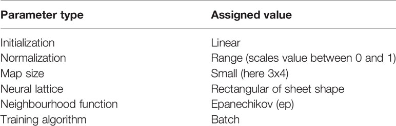
Table 1 SOM parameters and their optimal assigned values based on Liu et al. (2006a).

It is also important to note that the pre-processing of the input dataset (here U, V, SST, Chl-a) includes an additional step before the normalizing of the data (Figure 2). We transform each re-gridded U (V, SST or Chl-a) image of the period Nov-Mar 1997-2020, into a single row vector by concatenating each row in the image. The final input vector consists of 3479 arrays (one for each day of the observational record) each of 4416 elements (1104 pixels *4 variables). We then remove non ocean pixels, following Richardson et al. (2003) and normalize data with a range normalization for each variable (so all the variables are between 0 and 1). Note that the possible data gaps in SST and Chl-a data due to cloud coverage, are dealt with by choosing products that are gap (cloud) free as already mentioned. Indeed, although the SOM algorithm can robustly handle data gaps (Liu et al., 2006b), using datasets with large number of gaps can lead to less realistic SOM outputs. Hence, for the Chl-a data, which is most affected by cloud coverage, we chose the GlobColour product which has L4 daily gap-free composites over the Ocean Colour - Climate Change Initiative (OC-CCI) product whose daily composites are L3 with higher number of missing data. The SOM algorithm uses the daily normalized multivariate vectors (U, V, SST, Chl-a which are moving in a 2D space (longitude, latitude) and in time (days - 1D) to perform the clustering analysis and retrieve the dominant spatial patterns. The SOM approach is summarized in Figure 2.

3 Results

3.1 Patterns Classification: AC Modes

The extracted SOM spatial patterns summarize the currents, SST and Chl-a variability for the period Nov-Mar 1997-2020 (Figures 3, 4 and Supplementary Figures 2, 3) over the study region (cf. section 2.2.1 and Figure 1, orange box). Here, we first analyse the SOM outputs focusing on the currents’ variability and their dominant topologies or modes during the observational record. A schematic of the currents’ direction and speed (along with the corresponding SST) is presented superimposed to current vectors (plotted every 2 grid points) in Figure 3 and separately in Supplementary Figure 4 for better clarity. Note that the difference in current speed over the Bank, which is masked by the much stronger AC, was determined using additional plots with a colour-scale set at a maximum of 0.5 m/s to clarify the flows there (Supplementary Figures 3, 5). As already mentioned, the SOM outputs (Figures 3, 4) are arranged in such a way that close patterns, which represent similar weight vectors, are neighbouring each other, while dissimilar patterns, which correspond to different weight vectors, are distant from each other (Jouini et al., 2016; Liu et al., 2016). The percentages (Figures 3, 4 and Supplementary Figures 2, 3) indicate the frequency of occurrence of each SOM pattern during the 23 years of observations. The frequency of occurrence is calculated here following the Liu et al. (2016) method, where the number of times a pattern was selected as a BMU is divided by the BMU timeseries length. Each pattern and percentage correspond to a dynamical signal. They indicate a certain type of circulation, SST and Chl-a distribution. However, some of these patterns share similarity in terms of the AC configuration and overall circulation. The 12 characteristic spatial currents and SST patterns show similar ARC meanders (solid green arrows), except in P6 where the ARC is located farther south, and eddies southwest (solid grey arrows) and southeast (dashed green arrows) off the Bank (Figure 3). The latter likely originated from the flow around Madagascar (e.g., Ridderinkhof et al., 2013). All the patterns (12 maps) show a main AC entering the Bank from 3 locations (the east at ~24°E and 35°S, centre at ~35.2°E and 22.5°S and southwest at ~20.9°E and 36.2°S), but with some significant differences in the circulation over the Bank (Figure 3). The eastern Bank experiences a return flow directed northeast in every pattern, however, in P5 this flow meanders to the east and then southwest (dashed pink arrows, Figure 3). On the western Bank, the current meanders northeastward then northwestward, except in P6 where it only flows northeastward (dashed blue arrows, Figure 3). Part of this northeast-northwest meandering flow, circles back in a cyclonic loop (dotted blue arrows, Figure 3), excluding P5, P9 and P12. The flow on the central Bank is mainly southwestward, with a slight difference in P9 where it flows northwestward before meandering southwestward.

FIGURE 3

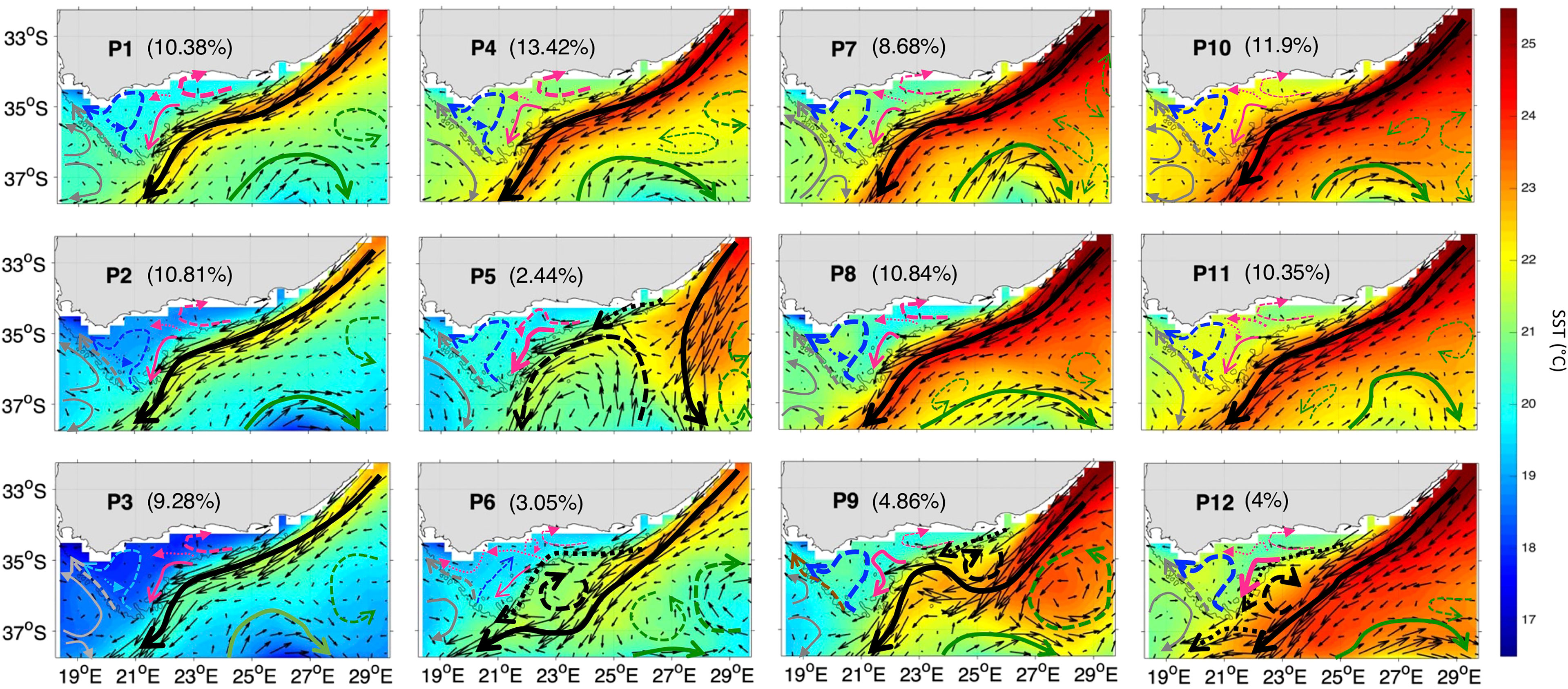
Figure 3 The 12 characteristic SST (in °C) and surface currents patterns (P1 to P12) over the Agulhas area of interest (orange box, Figure 1) during Nov-Mar 97-20 as derived from the 3x4 SOM. The current vectors (thin black arrows) are mapped every 2 grid points. The stronger the currents the longer are the vectors. A schematic of the currents’ direction and speed during Nov-Mar 97-20 for 12 SOM patterns (P1 to P12) is superimposed. The black arrows represent the main AC and its associated meanders. The green (grey) arrows designate the main circulation southeast (southwest) off the Bank. The blue (pink) arrows indicate the circulation on west (east and central) Bank. The stronger the currents the thicker are the arrows. The percentages between parentheses represent the frequency of occurrence of each pattern. The 200m isobath marking the continental shelf is highlighted with a grey solid line.

FIGURE 4

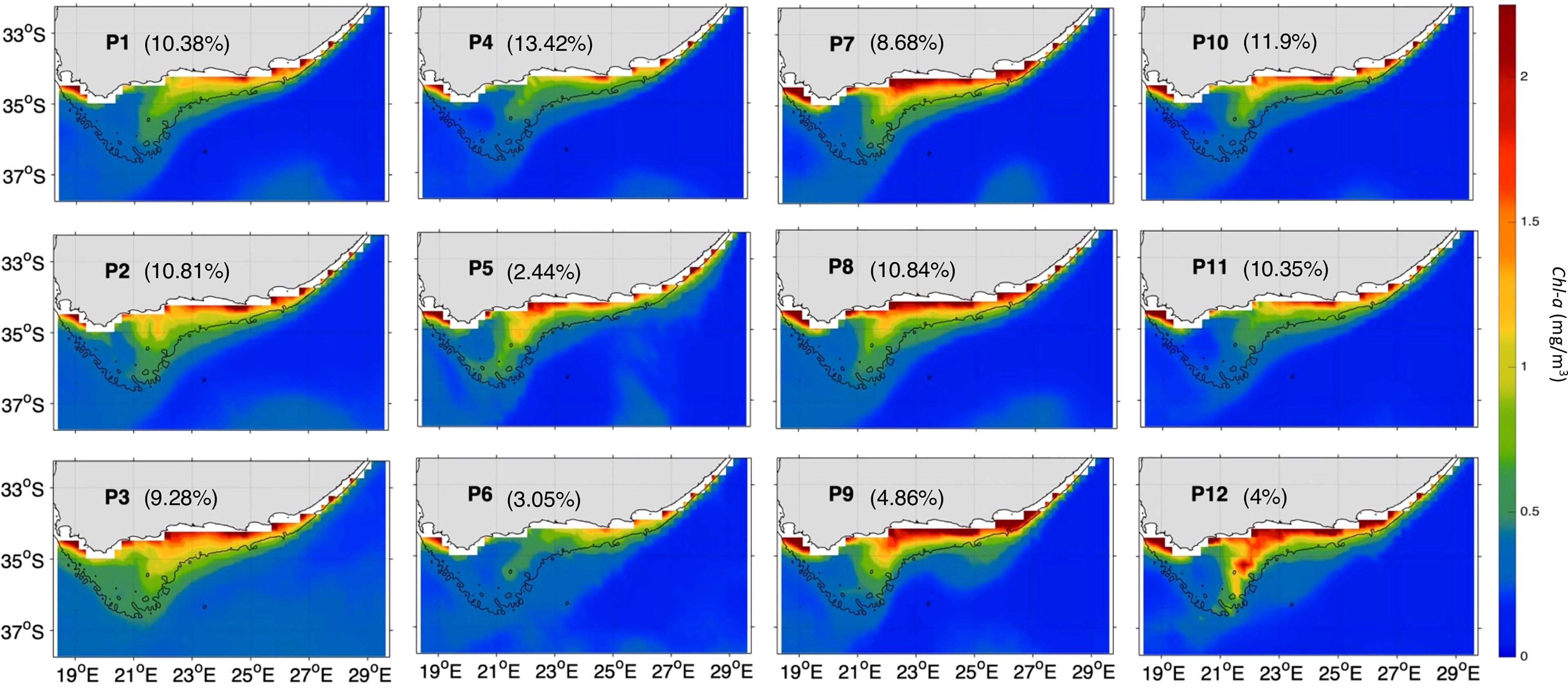
Figure 4 The 12 characteristic Chl-a (in mg/m³) patterns (P1 to P12) over the Agulhas area of interest (orange box, Figure 1) during Nov-Mar 97-20 as derived from the 3x4 SOM. The currents vectors are plotted with the same length, so the direction of the currents is clearer. The currents speed can be seen from the colormap. The percentages between parentheses represent the frequency of occurrence of each pattern. The 200m isobath marking the continental shelf is highlighted with a black solid line.

The 12 SOM patterns display differences in the AC configuration as well (in terms of magnitude and the current pathways) that appear to influence the circulation over the Bank (Figure 3), and possibly affect the advection of nutrients and hence phytoplankton growth (e.g., Jebri et al., 2020). These SOM patterns can be categorized into 4 modes based on the main AC configuration (dashed and solid thick black arrows, Figure 3): AC along the shelf edge (P1-4, P7-8, P10-11), AC early retroflection (P5), AC with a cyclonic meander off shelf of the east and central bank (P6) and AC with a cyclonic meander near shelf (P9, P12) (Table 2). The AC along the shelf edge mode spans the left and upper right sides of the SOM (P1-4, P7-8, P10-11) and is identified by a main AC flowing south-westward along the topography. This AC topology is the most frequent (85.66% of the observational record), but the current can appear narrow and cool (P1-3), which includes ~30.47% of the realizations or broader and warmer (P4, P7-8, P10-11) occurring ~55.19% of the time (Figures 3). The AC early retroflection mode (P5) exhibits an early retroflection of the AC, which is much farther to the east (around 27.5°E while it usually occurs at 18-20°E, Russo et al., 2021), and a large anticyclonic meander (dashed black arrow) centered at 37.4°S and 23.5°E, which detached from the retroflected AC (Figures 3). This mode is the least frequent with only 2.4% occurrences during the 23 years. The AC with cyclonic meander off shelf (P6) occurs rarely with only ~3.05% of the AC realizations during the study period and is characterized by an AC meandering away from the shelf with a cyclonic eddy, centered at 36°S (dashed black arrow), which likely corresponds to a Natal pulse (e.g., Lutjeharms, 2006). The AC with cyclonic meander near shelf, spanning the lower right corner of the SOM (P9, P12), is apparent 8.86% of the time and exhibits an AC flowing near the shelf with a cyclonic eddy, centred at 35°S in P9 and at 35.7°S in P12, which also could be a Natal pulse (e.g., Lutjeharms, 2006). Note that this approach of grouping the patterns into variability modes is commonly used when interpreting SOM outputs in oceanographic studies (e.g., Liu et al., 2016).

TABLE 2

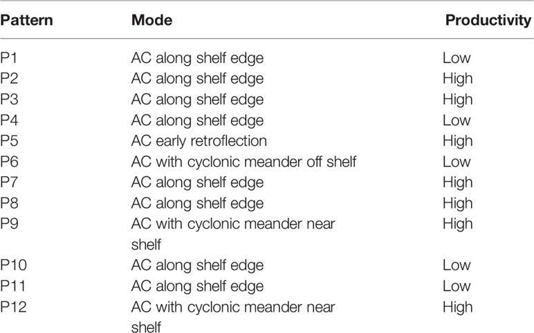
Table 2 Summary of the SOM current patterns classification and their associated productivity state.

3.2 Link to SST and Phytoplankton Biomass Over the Cold Ridge (Central Agulhas Bank)

In this section, the main AC modes are further examined in relation to SST and Chl-a variability along the Cold Ridge path (central Agulhas Bank). Strong Cold Ridge upwelling indicated by prominent phytoplankton biomass and lower SST, relative to the surrounding waters, is the dominant condition. It is observed in the AC early retroflection mode (P5), the AC with a cyclonic meander near shelf mode (P9 and P12) and half of the AC along the shelf edge patterns (P2-3 and P7-8) (Figures 3, 4). The Chl-a and SST signature of the seasonal Cold Ridge upwelling can be diminished, such as in the AC with a cyclonic meander off shelf mode (P6) and in the remaining patterns of the AC along the shelf edge mode (P1, P4, and P10-11) (Figures 3, 4). These changes in SST and Chl-a over the Bank can be linked to the interplay between the intensity and/or direction of the flow on the eastern Bank (dashed pink arrows), central shelf (solid and dotted pink arrows) and western Bank (blue arrows) (Figures 3, 4).

In the AC along the shelf edge mode, P2-3 show the coolest SST overall and specifically over the Cold Ridge path (down to ~18-18.5°C), and a high (~1.25-2.25 mg/m³) widespread phytoplankton biomass over the Bank, indicating a stronger upwelling (Figure 3, 4). However, their circulation patterns are similar to the less productive P10-11, which show a narrower Cold Ridge extension (both in terms of Chl-a and SST) (Figures 3, 4). The main difference lies in the southwestward flow on the central Bank in P10-11 being the second weakest (after P6) among all patterns (solid pink arrow, Figure 3), which can indicate a weaker advective effect along the Cold Ridge, thus smaller horizontal extension of Chl-a. The northwestward flow on the central Bank is also stronger in P10-11 than in P2-3 (thick dotted pink arrows, Figure 2), which suggests a stronger advective effect towards the western Bank in P10-11. The SOM P1 and P4 patterns show the second coolest SST but appear less productive (i.e., high Chl-a levels remain confined to the coast) than their neighbouring P2 pattern (Figures 3, 4). Their northeast circulation is the strongest (dashed pink arrows, Figure 3), which might hinder the extension of the cold and high Chl-a waters farther to the southwest than in P2 (Figure 4). Patterns P7-8 display high Chl-a values (>2.25 mg/m³) which extend farther from the coast compared to P10-11 (Figure 4). Indeed, the SST appears cooler (by ~1°C) over the Cold Ridge area in P7-8 than in P10-11, suggesting a stronger upwelling (Figure 3). Additionally, the southwestward flow is stronger in P7-8 than P10-11, (solid pink arrow, Figure 3) indicative of a wider horizontal extension of the Cold Ridge, despite the northeast flow on the eastern Bank being slightly stronger in P7-8 than P10-11 (dashed pink and blue arrows, Figure 3).

In the AC early retroflection mode (P5), the high Chl-a levels (~1.25-2.25 mg/m³) and low SST (~19.5°C) extending southwestward over the Cold Ridge path (Figures 3-4) are associated with the second strongest (after P12) southwestward flow over the central Bank (solid pink arrow, Figure 3). This southwestward circulation is fed by an eastward flow originating (dashed pink arrow), from part of the fast AC (dotted black arrow) which enters the eastern Bank, and the anticyclonic meander (dashed black arrow), which detached from the early reflected AC (solid thin black arrow) (Figure 3).

The lowest Chl-a values over the Cold Ridge path (with maximums of 0.75-1.2 mg/m³) are seen in the AC with a cyclonic meander off shelf mode (P6) (Figure 4). This is likely due to southwestward flow (solid pink arrow) over the central Bank being weakest in P6 (Figure 3), which does not favour extension of the Cold Ridge southwestward. Another unique feature in P6, is that the part of the AC (dotted black arrow) north of the cyclonic meander enters the Bank around 23°E and 35°S and flows westward (dotted pink arrow) until the west Bank coast, which can also restrain the extension of the Cold Ridge. In contrast to P6, when the AC meanders and a cyclonic meander (or Natal pulse) lies near the shelf (i.e., AC with a cyclonic meander near shelf mode, P9 and P12) a strong Cold Ridge in terms of high Chl-a values (1.5 to above 2.25 mg/m³) and south-westward horizontal extent occurs (Figures 3, 4). The large south-westward extent of the Cold Ridge in P9 and P12 (Figure 4) is likely due to the weak northeast circulation on the eastern Bank and the intense southwest flow over the central Bank (solid pink arrows, Figure 3). This southwest flow over the central Bank is strongest in P12, leading to the most south-westward extension of the Cold Ridge, and third strongest in P9 (of a similar intensity to the productive P7-8) (Figure 3). A summary of the currents’ patterns classification and their associated productivity state is given in Table 2.

3.3 Interannual Variations of the Surface Current, SST and Chl-a Patterns

3.3.1 Typical Conditions

To better understand the year-to-year evolution of the extracted 12 spatial patterns over the period Nov-Mar 1997-2020, we next analyse the BMU timeseries returned by the SOM (Figure 5A). It shows pronounced variability with some anomalous events differing significantly from the rest of the timeseries (Figure 5A). Indeed, by comparing the 12 patterns with the input data maps (daily snapshots), a BMU can be found for each input data vector (e.g., Liu et al., 2016). From the BMU timeseries, the characteristic progression of the SOM patterns (i.e., the typical (most common) pattern sequence) on the SOM grid can be seen to be exemplified by the 2016-17 pattern sequence (Figures 5A). The 2016-17 zoomed-in BMU timeseries and associated patterns provide a detailed visualization of the typical pattern trajectory (Figures 5B, 6 and 7). It is solely composed of the AC along the shelf edge mode (Figures 5B, 6 and 7) which spans P3, P2, P1 and P4; then P11, P7, P8, and P10. Note that in Figures 6, 7, the frequency of occurrence associated with each pattern is indicated relative to the length of the time recorded during Nov-Mar 2016-17 only. Note also that the patterns sequence (trajectory) is determined from the BMU timeseries variations (Figure 5), where the patterns P1-12 (vertical axis) move with time (horizontal axis). Since the SOM grid is composed of 12 patterns arranged from top to bottom (e.g., P1-P2-P3) and from left to right (e.g., P1-P4-P7-P10), it is possible to tell if the SOM is spanning the left or right corner or centre part of the grid when looking at the BMU timeseries (Figure 5). The typical pattern trajectory spans first the left side of the SOM (P3→P2→P1→P4), moving from a cool and high Chl-a Agulhas Bank (P3 → P2) in November to a relatively warmer and less productive configuration (P1 → P4) in December (Figures 6, 7). Next, the patterns move back and forth across the SOM upper right nodes (P11→P7→P11→P8→P11→P10→P8) with overall warmer SST than P1-4. P11, P7 and P8 are seen in January, with P11 being most frequent and least productive in comparison to P7-8 (P7 lasts for 5 days in early January and P8 for 9 days in mid-January). P11, P10 and P8 appear in February. P11 makes up the first three-quarters of February, while P10 (for 5 days) followed by P8 (3 days) appear in the last quarter of February. In March, only the productive pattern P8 is active. The most dominant pattern (P8), with 28.48% frequency of occurrence, is associated with high Chl-a and low SST over the central Bank (Cold Ridge path). But overall, the patterns oscillate, with about 50-50 chance, between less productive (P1, P4 and P10-P11, occurring 50.34% of the time) and more productive (P2-3 and P7-8, making up 49.66% of the realizations) Cold Ridge upwellings.

FIGURE 5

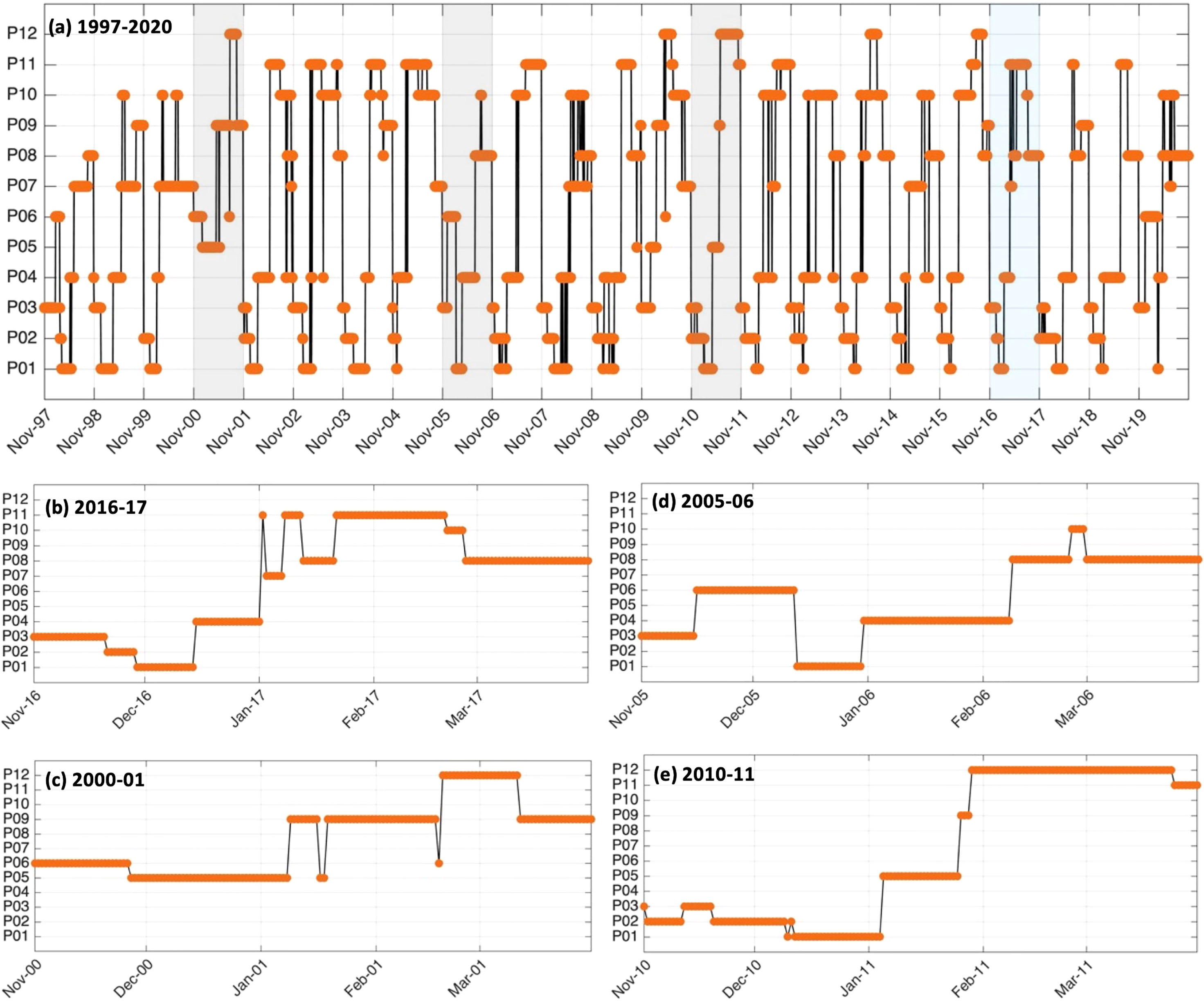
Figure 5 BMU timeseries indicating the daily evolution the SOM 12 patterns (P1 to P12) during all Nov-Mar (A) 1997-2020, a typical patterns’ sequence (B) 2016-17 and the anomalous events (C) 2000-01, (D) 2005-06 and (E) 2010-11.

FIGURE 6

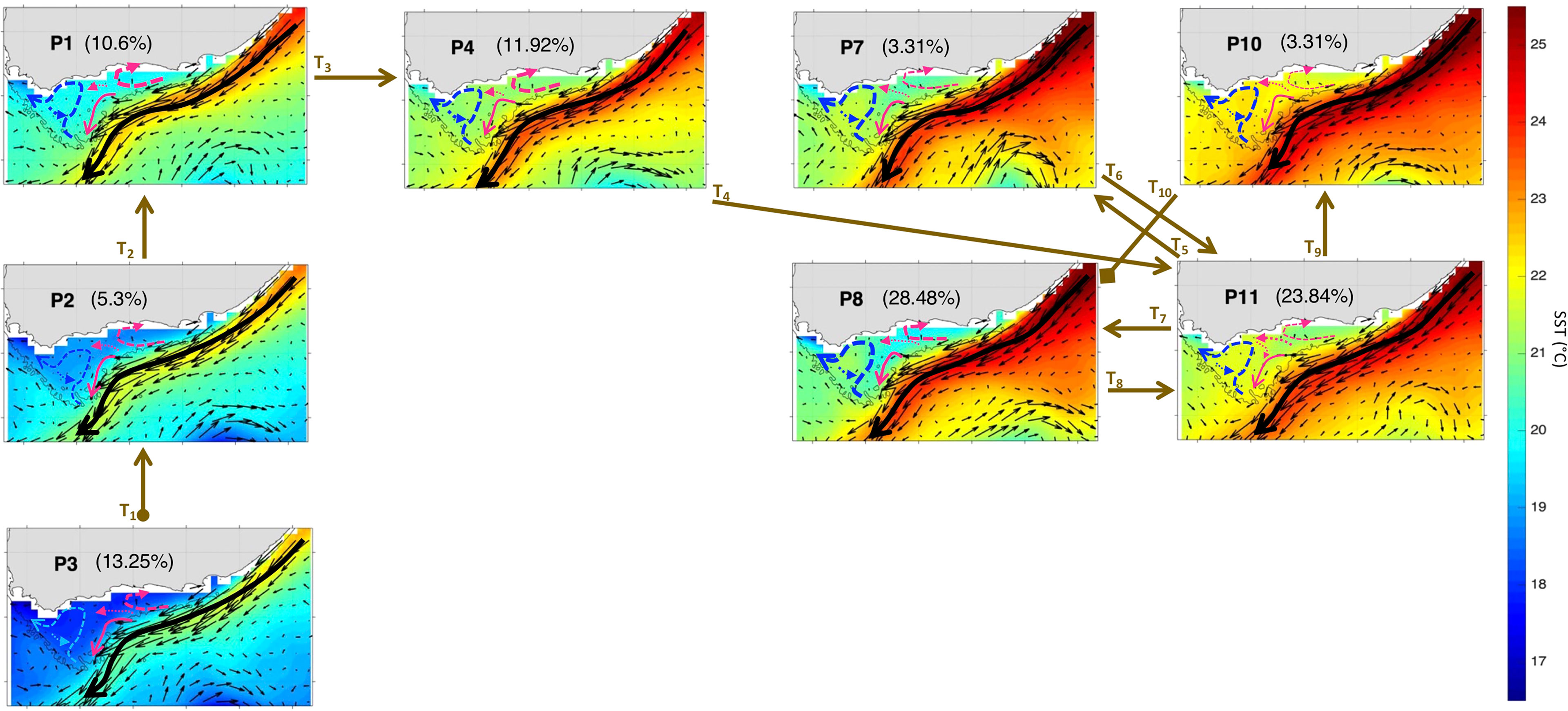
Figure 6 Same as Figure 3 but for Nov-Mar 2016-17. The frequency of occurrence of each pattern is calculated here relative to the days recorded during Nov-Mar 2016-17. The brown arrows represent the SOM patterns trajectories (T_i=1:10) evolving during Nov-Mar 2016-17as inferred from the BMU timeseries (Supplementary Figure 4A). The starting (final) trajectory is designated with a circle (diamond) at the arrow beginning (end).

FIGURE 7

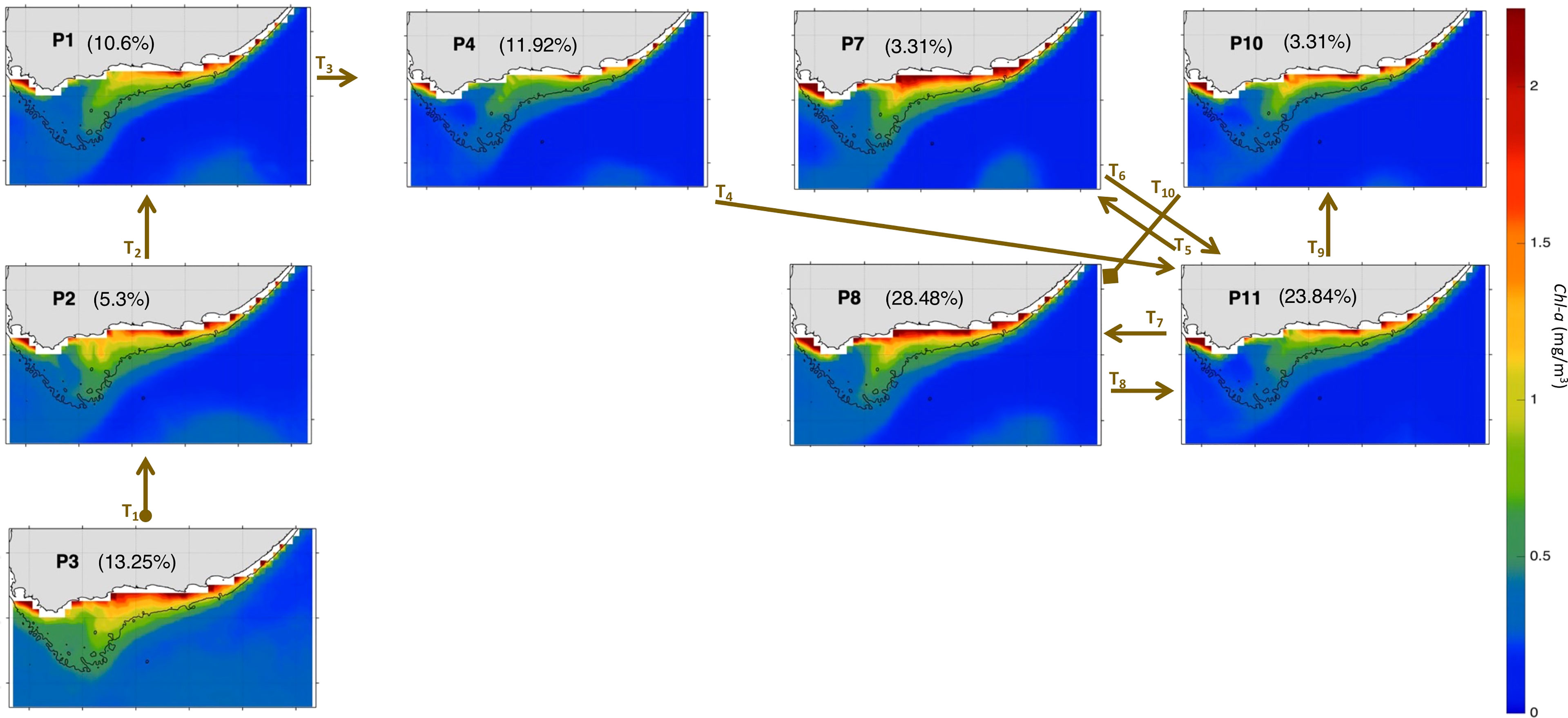
Figure 7 Same as Figure 4 but for Nov-Mar 2016-17. The frequency of occurrence of each pattern is calculated here relative to the days recorded during Nov-Mar 2016-17. The brown arrows represent the SOM patterns trajectories (T_i=1:10) evolving during Nov-Mar 2016-17 as inferred from the BMU timeseries (Supplementary Figure 4A). The starting (final) trajectory is designated with a circle (diamond) at the arrow beginning (end).

3.3.2 Anomalous Conditions

In contrast to Nov-Mar 2016-17 (typical season), the active patterns evolution was most anomalous/unusual (i.e., with a patterns’ sequence significantly different from the typical sequence) during 2000-01, 2005-06 and 2010-11 upwelling seasons (Figure 5A). Note that other years were also quite irregular, namely 1997-98 and 2019-20 (see Supplementary Figures 6–10), compared to the rest of the time record (Figure 5A) and these are discussed in section 4 below.

The anomalous patterns’ trajectory of Nov-Mar 2000-01 revealed by the zoomed-in BMU timeseries (Figure 5C) spans four patterns (P5, P6, P9, P12), which compose the AC early retroflection (P5), AC with cyclonic meander off shelf (P6) and AC with cyclonic meander near shelf (P9, P12) mode, while typical conditions show only the AC along the shelf edge mode for eight patterns (Figures 5C, 8 and 9). The patterns sequence in November 2000 begins at the SOM centre spanning P6→P5 (Figures 5C, 8 and 9), instead of the usual SOM bottom left side (P3→P2 in a typical November, Figures 5B, 6 and 7). In Nov 2000, the SOM is in the AC with cyclonic meander off shelf mode (P6), except for the last 4 days where it moved to the AC early retroflection mode (P5). The AC system remained in P5 for all of December 2000 and until early January 2001. During the rest of January 2001, the SOM moves down to the AC with cyclonic meander near shelf mode (P9), except for 2 days by ~mid-month where P5 took place. The AC with cyclonic meander near shelf mode continues to dominate during February 2001, with mainly P9 and P12 occurring (though P6 was on for a day by mid-February) during the first and second halves of the month, respectively. These patterns (P12 then P9) were also the active patterns of March 2001. The AC with cyclonic meander off shelf mode (P6), which correspond to a weak Cold Ridge (in terms of Chl-a values and horizontal extent, cf. section 3.2) occupied 17.88% of the realizations during Nov-Mar 2000-01. P12, which leads to the most south-westward extended Cold Ridge, was the least dominant (13.9%) during that period. But, overall, the high-productive patterns (P5, P9 and P12, cf. section 3.2) represent together about 82.12% of the 2000-01 occurrences. Thus, Nov-Mar 2000-01 was mainly a high productive season (with 82.12% frequency of occurrence of the more productive patterns) over the Agulhas Bank, in agreement with Jebri et al. (submitted).

FIGURE 8

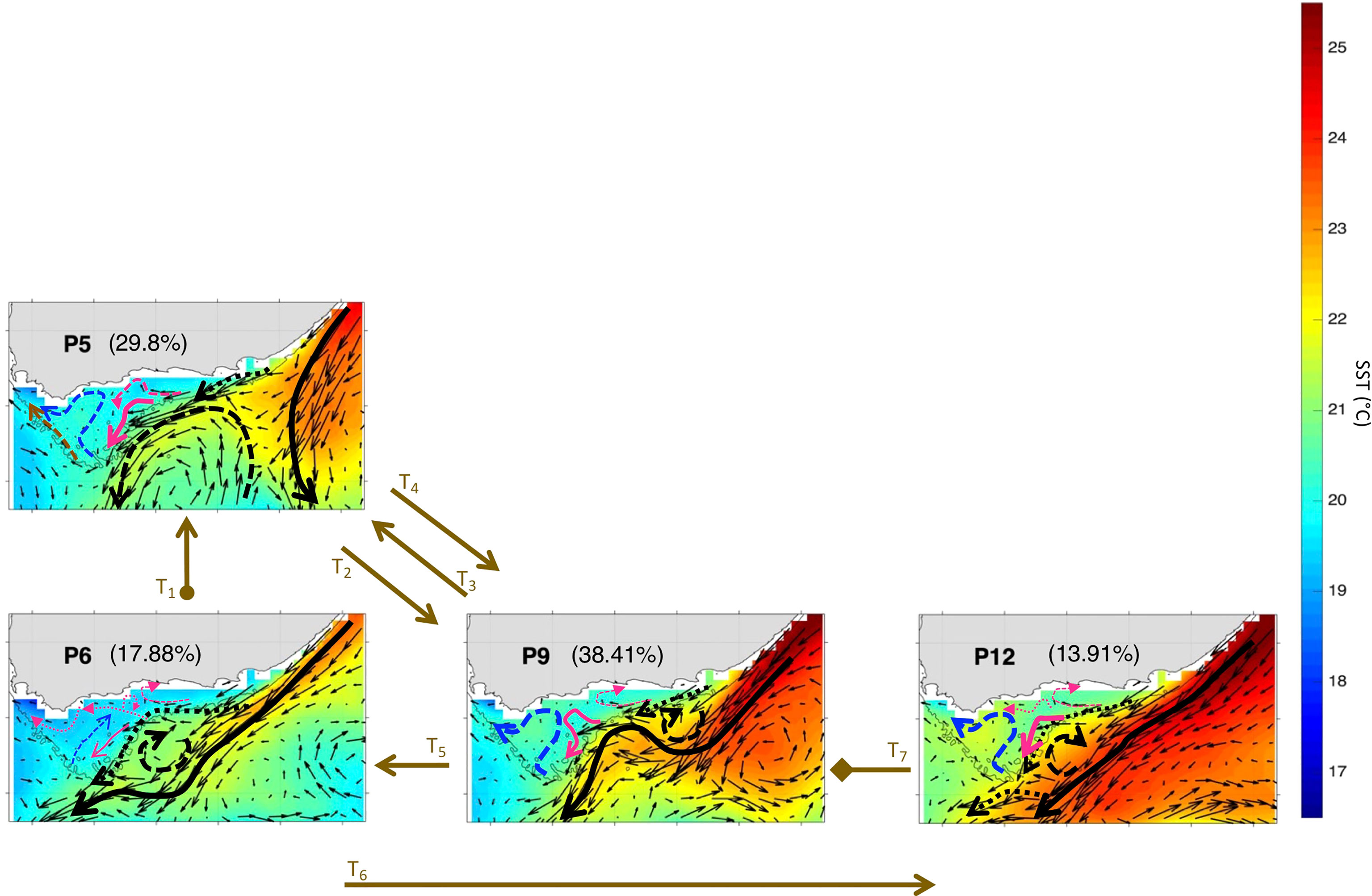
Figure 8 Same as Figure 3 but for Nov-Mar 2000-01. The frequency of occurrence of each pattern is calculated here relative to the days recorded during Nov-Mar 2000-01. The brown arrows represent the SOM patterns trajectories (T_i=1:7) evolving during Nov-Mar 2000-01 as inferred from the BMU timeseries (Supplementary Figure 4A). The starting (final) trajectory is designated with a circle (diamond) at the arrow beginning (end).

FIGURE 9

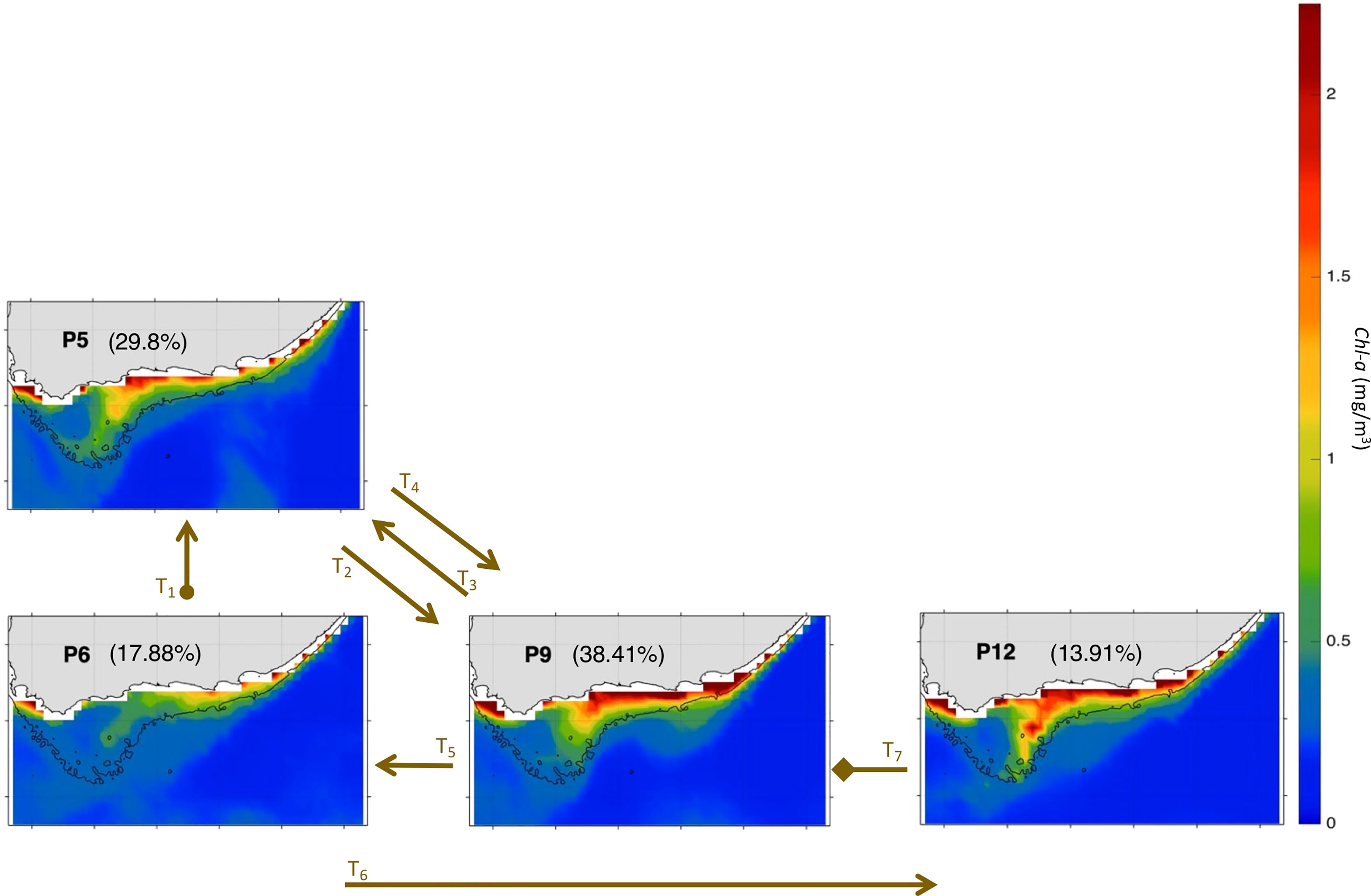
Figure 9 Same as Figure 4 but for Nov-Mar 2000-01. The frequency of occurrence of each pattern is calculated here relative to the days recorded during Nov-Mar 2000-01. The brown arrows represent the SOM patterns trajectories (T_i=1:7) evolving during Nov-Mar 2000-01 as inferred from the BMU timeseries (Supplementary Figure 4A). The starting (final) trajectory is designated with a circle (diamond) at the arrow beginning (end).

Nov-Mar 2005-06 sequence displays 6 patterns belonging to the AC along shelf edge mode (P1, P3, P4, P8, P10) and the AC with a cyclonic meander off shelf (P6) (Figures 5D, 10 and 11). This sequence initiates at the SOM bottom left corner, spanning P3 then P6 during the first and second half of Nov 2005, respectively, while a typical November sees P2 after P3 (Figures 5D, B). The AC with a cyclonic meander off shelf mode (P6) continues until ~mid Dec 2005 before the SOM moves up to P1 which lasts until the end of month, except the last day where the usual P4 appears. P4 then dominates all of Jan 2006 instead of P11, P7 and P8 occurring in a typical January. The patterns trajectory spans the SOM right side in Feb 2006, moving from P4→P8→P10 (P11→P10→P8 in typical Feb). In Mar 2006 appears the same as a typical March with only P8 is active. The pattern with the most realizations (31.13%) in Nov-Mar 2005-06 is P8 (Figures 10, 11), which indicates strong Cold Ridge upwelling (cf. section 3.2). However, patterns P1, P4, P10 and P6, indicative of low productivity over the Bank, represent the majority with 58.94% of occurrences during 2005-06 upwelling season (Figures 10, 11). This makes the Nov-Mar 2005-06 event mostly low productivity (with 41.06% frequency of occurrence of the more productive patterns).

FIGURE 10

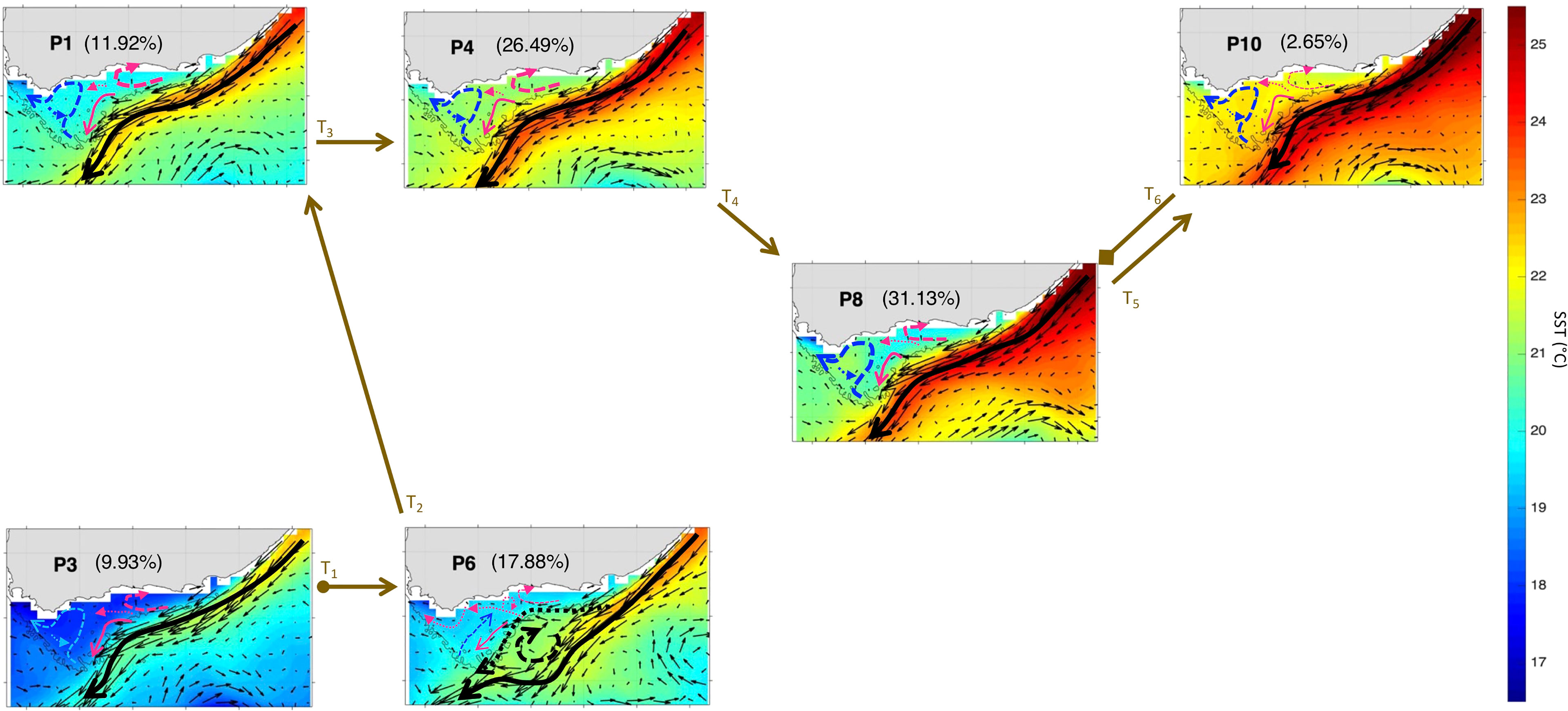
Figure 10 Same as Figure 3 but for Nov-Mar 2005-06. The frequency of occurrence of each pattern is calculated here relative to the days recorded during Nov-Mar 2005-06. The brown arrows represent the SOM patterns trajectories (T_i=1:6) evolving during Nov-Mar 2005-06 as inferred from the BMU timeseries (Supplementary Figure 4A). The starting (final) trajectory is designated with a circle (diamond) at the arrow beginning (end).

FIGURE 11

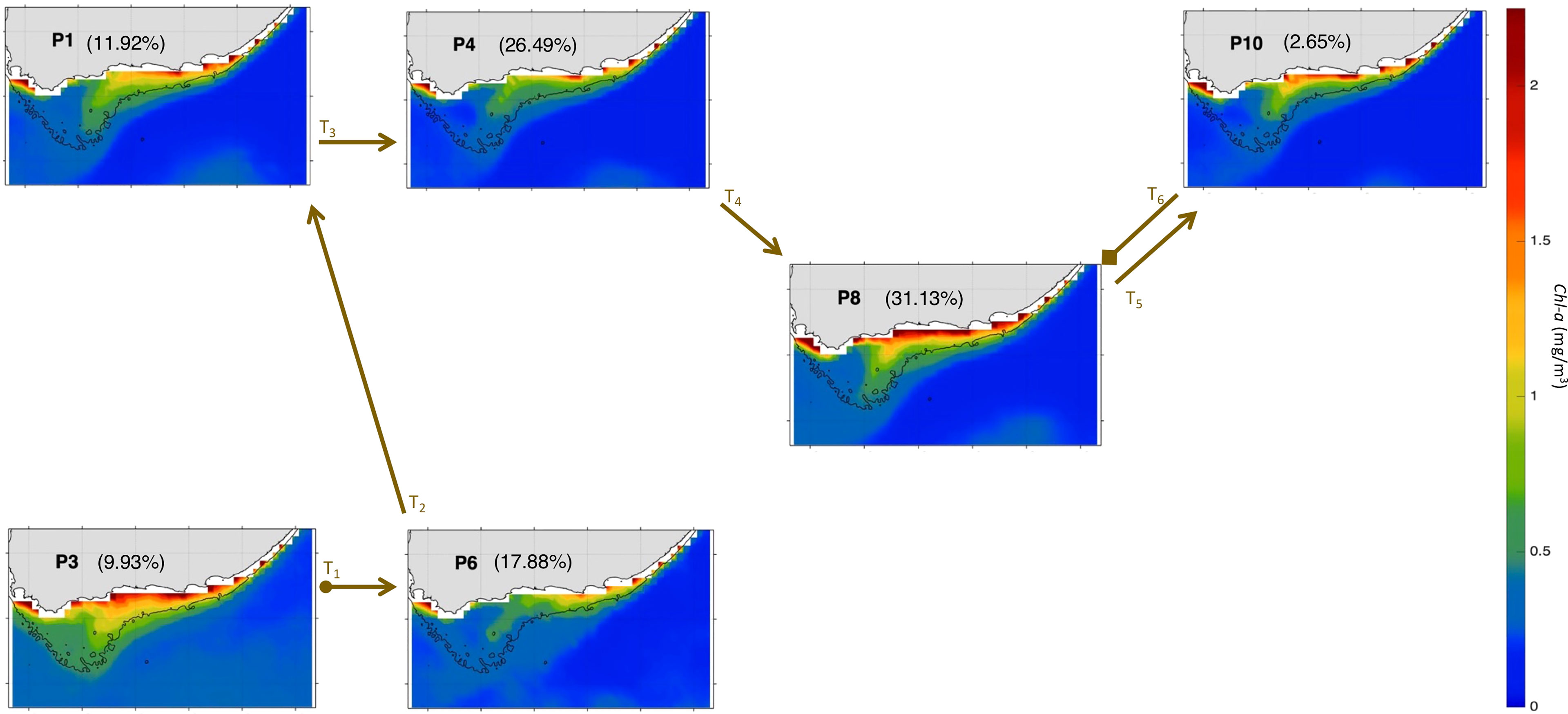
Figure 11 Same as Figure 4 but for Nov-Mar 2005-06. The frequency of occurrence of each pattern is calculated here relative to the days recorded during Nov-Mar 2005-06. The brown arrows represent the SOM patterns trajectories (T_i=1:6) evolving during Nov-Mar 2005-06 as inferred from the BMU timeseries (Supplementary Figure 4A). The starting (final) trajectory is designated with a circle (diamond) at the arrow beginning (end).

Nov-Mar 2010-11 experienced a more complicated AC patterns evolution (Figures 5E, 12 and 13) than 2000-01 and 2005-06. From Nov to Dec 2010, the AC flowing along the shelf edge was dominant (43.05%) with two repetitions of P3→P2 in Nov 2010 and of P2→P1 in Dec 2010. This Nov and Dec patterns sequence (Figure 5E) is different from typical conditions which see P3→ P2 once in Nov and P1→P4 once in Dec (Figure 5B). Except for the first 4 days where P1 is still active, the SOM path evolved diagonally across the grid during Jan 2011, from the AC early retroflection (P5→) to the AC near shelf with cyclonic meander mode (P9→P12) (Figures 12, 13). The SOM trajectory remains at the bottom right SOM corner, in P12, during Feb and Mar 2011, excluding the last week of Mar 2011 where the SOM moves up to the AC flowing along the shelf edge (P11). Overall, P1 and P11, from the AC along the shelf edge mode, which are associated with low productivity over the Bank, represent only 21.2% of the occurrences during 2010-11. The rest of the 2010-11 patterns (P2-3, P5, P9 and P12), which are indicative of strong Cold Ridge upwelling and high Chl-a levels (cf. section 3.2), represent 78.8% of the realizations during the same period. Hence, Nov-Mar 2010-11 was mainly highly productive (with 78.8% frequency of occurrence of the more productive patterns).

FIGURE 12

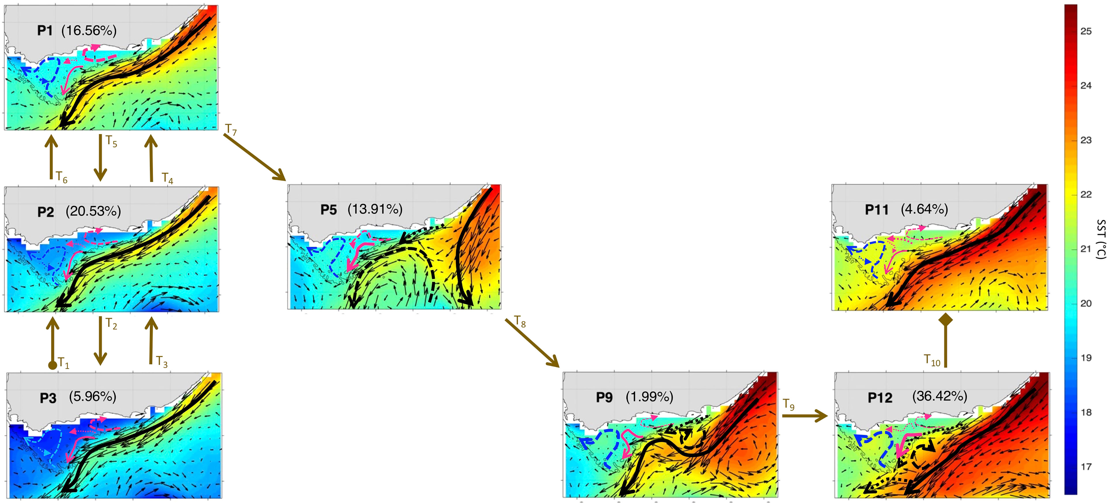
Figure 12 Same as Figure 3 but for Nov-Mar 2010-11. The frequency of occurrence of each pattern is calculated here relative to the days recorded during Nov-Mar 2010-11. The brown arrows represent the SOM patterns trajectories (T_i=1:10) evolving during Nov-Mar 2010-11 as inferred from the BMU timeseries (Supplementary Figure 4A). The starting (final) trajectory is designated with a circle (diamond) at the arrow beginning (end).

FIGURE 13

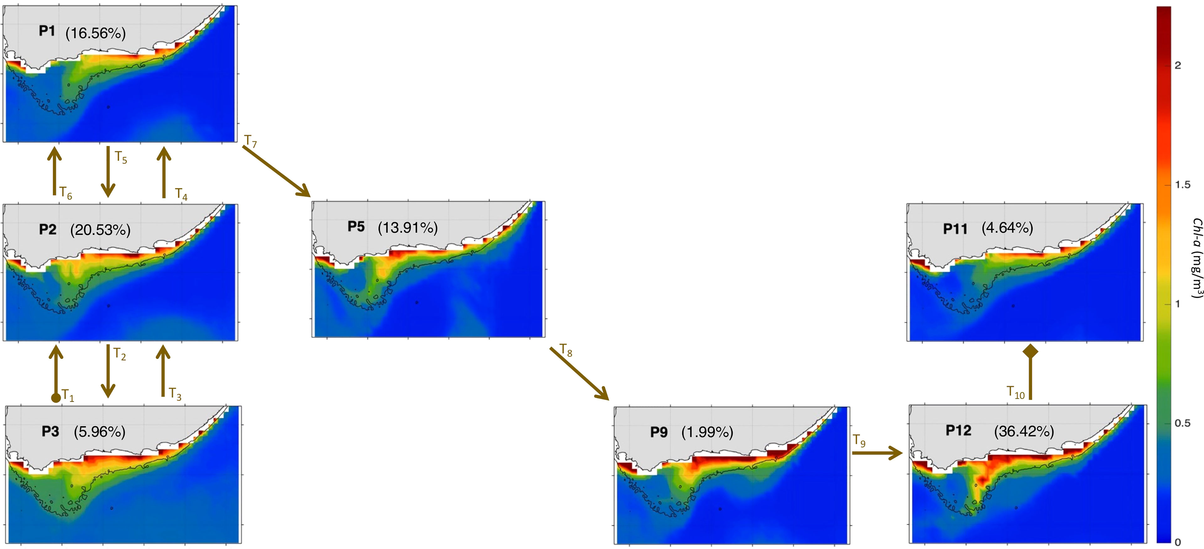
Figure 13 Same as Figure 4 but for Nov-Mar 2010-11. The frequency of occurrence of each pattern is calculated here relative to the days recorded during Nov-Mar 2010-11. The brown arrows represent the SOM patterns trajectories (T_i=1:10) evolving during Nov-Mar 2010-11 as inferred from the BMU timeseries (Supplementary Figure 4A). The starting (final) trajectory is designated with a circle (diamond) at the arrow beginning (end).

3.3.3 Trends in the Frequency of Occurrence

There is an overall decreasing (increasing) trend in P1, P7 and P9 (P2, P4, P8) frequency of occurrence during the 23 years of observations (Figure 14). No clear trend is depicted in the rest of the SOM patterns (i.e., P3, P5, P6, P10, P11, P12) with slope values around zero (Figure 14). The most pronounced positive (negative) trend is seen in P8 (P7) with a slope value of 1.002 (-0.927). All these patterns correspond to the AC along the shelf edge mode, except for P9 which represent the AC with a cyclonic meander near shelf mode. This suggests that the occurrence of the AC along the shelf edge mode is mostly increasing while that of the AC with a cyclonic meander near shelf mode is tending to decrease (as P9 occurred more often than P12 overall, Figure 3) in the past 23 years. P2 and P8 (P4) are associated with high (low) productivity (Table 2) and P7 (P1), which occur overall less than P1 (Figure 3), corresponds to high (low) productivity (Table 2). This finding with the trends’ behaviour depicted above (Figure 14) suggest that high (low) productivity due to the AC along the shelf edge mode is increasing (decreasing); inferred from P2 and P8 (P1). The decrease in occurrence of P9 (Figure 14), which characterizes high productivity (Table 2) and is overall more common than P12 (Figure 3), suggest that productive situations due to the AC with a cyclonic meander near shelf mode are tending to decrease. However, care must be taken in interpreting these trends, as these have been determined from the SOM patterns only for the Nov-Mar period each year because here the focus is on changes in Cold Ridge upwelling. AC changes may be occurring that might lead to different trends during other parts of the year.

FIGURE 14

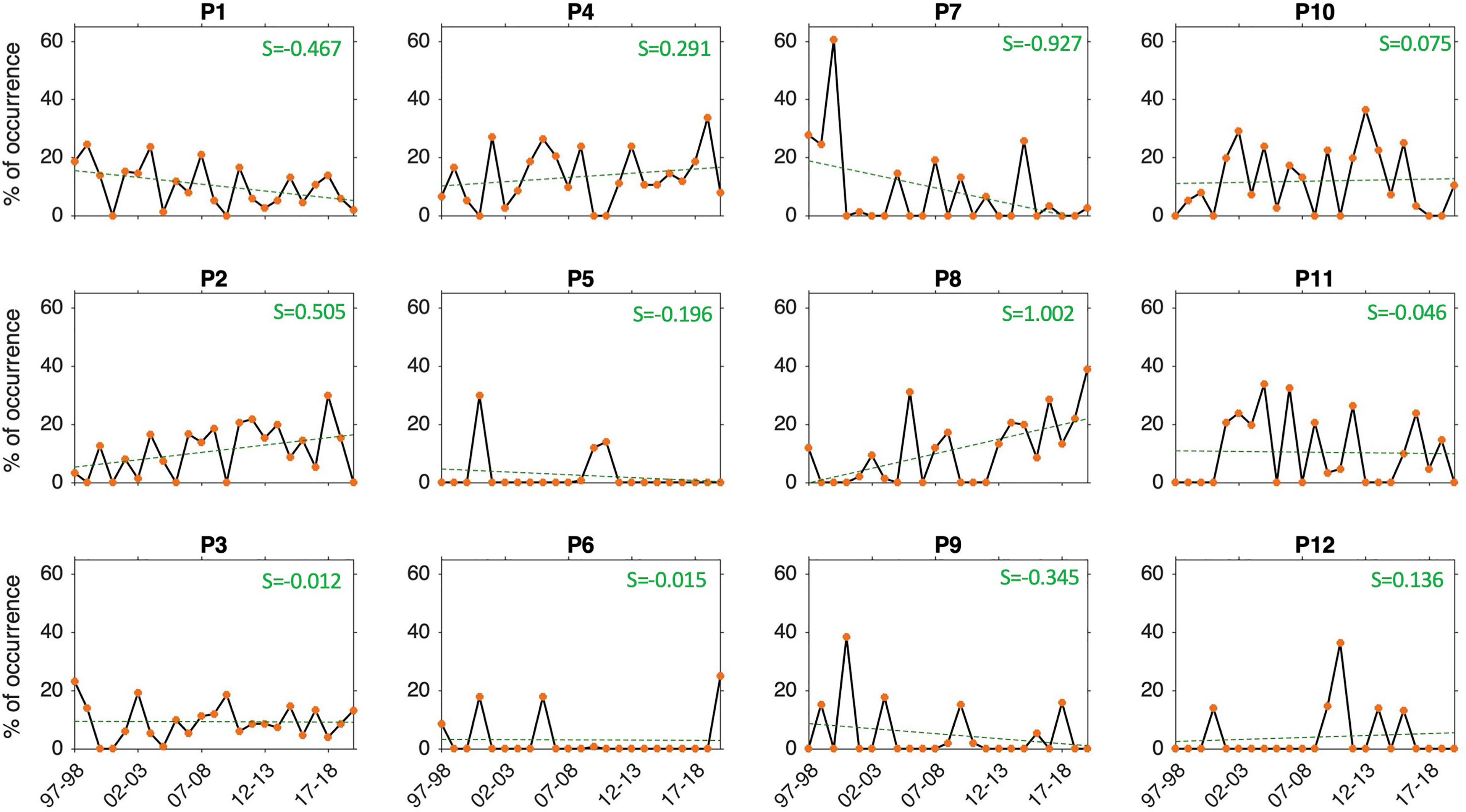
Figure 14 Time evolution of the frequency (%) of occurrence of the SOM 12 patterns (black solid lines with orange dots) and their linear trends (green dashed lines) during Nov-Mar 1997-2020. The slope values (S) of the linear trend lines is indicated in the green text. The frequency of occurrence of each pattern is calculated here relative to the days recorded during Nov-Mar of each year from 1997-98 to 2019-20.

4 Discussion

This study elucidates the variability of surface currents that are most significant during seasonal upwelling, and their influence on the phytoplankton biomass over the Agulhas Bank. This is particularly important because the surface currents’ typologies or modes, through their influence on phytoplankton productivity (Figures 3, 4), can also impact commercially valuable fisheries such as hake, anchovy, sardine, rock lobster and Chokka squid (Roberts, 2005; Brick and Hasson, 2016). The intrusion of AC waters onto the shelf (Figure 3) agrees with previous findings (Swart and Largier, 1987; Lutjeharms et al., 1989; Jackson et al., 2012) but the new result here is that it seems quasi-permanent during Nov-Mar. The eastward flow near the coast over the eastern/central Agulhas Bank (Figure 3) has been reported as sporadic from modelling analyses (Roberts and Mullon, 2010) rather than a prevailing feature. This eastward flow was also seen from drifters’ trajectories deployed in March 2008 (Hence it's stated Hancke et al ; their Figure 6A). The southwestward flow on the central Bank, along the Cold Ridge path (Figure 3), agrees also with previous works (Boyd and Shillington, 1994; Roberts, 2005; Jackson et al., 2012). However, the northeast then northwest circulation on the western Bank (Figure 3) are observed here for the first time. The dominant AC mode inferred from our SOM analysis (AC flowing south-westward along the topography P1-4, P7-8, P10-11, Figure 3), is known as the most common southern AC configuration (e.g., Lutjeharms, 2006). Our SOM classification shows also that the AC retroflection was much farther to the east in Dec-Jan 2000-01 (AC early retroflection mode, P5, Figure 3), in agreement with previous research based solely on direct observations (e.g., Quartly and Srokosz, 2002). The less frequent AC with cyclonic meander off (P6) and near shelf (P9, P12) modes (Figure 3) can result from the occurrence of a Natal pulse, which exerts a forcing on the current creating a meander (Jackson et al., 2012). When the AC and a Natal Pulse are near shelf, a strong southwestward flow is found over the east and central Bank (P9 and P12, Figure 3) and the phytoplankton biomass along the Cold Ridge path reaches its most southward extent (Figure 4). These P9 and P12 conditions are concurrent with the fact that a Natal pulse can be associated with strong productive events or intense upwelling over the Agulhas Bank (e.g., Krug et al., 2014; Jacobs et al., 2022). Additionally, a Natal pulse near the shelf can contribute to strengthening the part of the AC which enters the eastern Bank, generating transport offshore from the continental shelf (Jackson et al., 2012; Weidberg et al., 2015; Jacobs et al., 2022). In contrast, when the AC and a Natal pulse meander farther away from the shelf (P6, Figure 3), the flow over the east and central Bank is weak, in agreement with Jacobs et al. (2022), and the Chl-a over the Cold Ridge path is very low as only relatively high Chl-a concentrations remain along a small portion of the eastern Bank (24-24.5°E) (Figure 4). Interestingly, the trend in frequency occurrence of the SOM patterns over the past 23 years during the period Nov-Mar revealed that high productivity state due to the AC with a cyclonic meander near shelf mode is tending to decrease while high (low) productivity due to the AC along the shelf edge mode is increasing (decreasing) (Figure 14).

The interannual variations of the SOM currents and Chl-a patterns over the Agulhas region showed anomalous sequences (Figures 5A). These could be due to climate events, as oceanic phytoplankton productivity is known to respond to climate-driven variability modes (Behrenfeld et al., 2006; Cai et al., 2015; Racault et al., 2017). The El Niño Southern Oscillation (ENSO), for instance, drives the dominant atmospheric variance related to the interannual changes of AC transport (Schouten et al., 2002; Elipot and Beal., 2018) and can affect upwelling on the Agulhas Bank (Malan et al., 2019). Here, the Nov-Mar 1997-98 anomalous event, which coincides with the 1997-98 super El Niño and Intense IOD+ (e.g., Hameed et al., 2018), is found to be mostly productive (with 66.23% frequency of occurrence of the productive patterns, Supplementary Figures 6A, 7, 8). The closest to 1997-98 El Nino in terms of intensity during the study period, is the 2015-16 super El Nino (Hammed et al., 2018; Supplementary Figure 13A). However, Nov-Mar 2015-16 does not stand out as anomalous in the BMUs timeseries (Figure 5A; Supplementary Figures 6B) and displays a less productive season than 1997-98 (with 46.06% frequency of occurrence of the productive patterns) (Supplementary Figures 9, 10). The contrast between these two events can be explained by their different El Niño dynamics. In fact, 1997-98 was the strongest ever recorded Eastern Pacific (EP) El-Nino, while 2015-16 was the strongest to-date mixed EP and central Pacific (CP) El-Nino, which relies on basin-wide thermocline variations and subtropical forcing, respectively (Paek et al., 2017; Racault et al., 2017). This difference is important because an EP (CP) El Niño leads to an increase (decrease) in primary production and nutrients over the Agulhas Bank (the western most part of the Bank) (Racault et al., 2017, their Figure 6), which is coherent with our 1997-98 and 2015-16 findings (Supplementary Figures 7–10). During ENSO cold events (La Niña), wind-driven coastal upwelling, and hence phytoplankton growth, is favoured over the Agulhas Bank (Jury, 2020). This agrees with the mostly productive (78.8% frequency of occurrence of the more productive patterns) nature of 2010-11 anomalous event (Figures 12, 13), which coincided with the second most intense La-Nina on record since 1979 (e.g., Boening et al., 2012; Supplementary Figure 13A).

Both the ENSO mode and the Indian Ocean Diploe (IOD) can modulate the Agulhas retroflection and ring shedding (Schouten et al., 2002; De Ruijter et al., 2004; Beal et al., 2011). Their effects on the Agulhas system might occur with a delay (Quartly and Srokosz, 2002). The anomalous Nov-Mar 2000-01 event, which is mainly productive (with 82.12% frequency of occurrence of the productive patterns, Figures 8, 9), involved the occurrence of the rare early (i.e., extremely eastward) AC retroreflection mode (P5). This early retroflection, active from December 2000 to January 2001 (Figure 5C), was previously linked to the 1997-98 super El Niño and IOD+ delayed effect on the Agulhas retroflection and ring shedding (Quartly and Srokosz, 2002; Schouten et al., 2002; De Ruijter et al., 2004). Indeed, the extreme 1997- 98 El Niño and IOD+ resulted in the reduction of eddy formation in early 1999, which in turn prevented Agulhas rings shedding during the first half of 2000 (Quartly and Srokosz, 2002; Schouten et al., 2002). It also led to the propagation of a regular train of Madagascar eddy dipoles into the Agulhas region, massively impacting its retroflection, in the second half of 2000 (De Ruijter et al., 2004). This agrees with the unique circulation features seen in the AC early retroflection mode, including the anticyclonic meander/ring detached from the main AC which contributes to the strong south-westward flow (extended Cold Ridge) over the central Bank (P5, Figures 3, 8).

Another anomalous event in the BMUs timeseries which can be linked to extreme IOD is Nov-Mar 2019-20 event (Figure 5A). The autumn (October-November) of 2019 experienced the second strongest IOD+ between 1979 and 2020 (Wang et al., 2020, Supplementary Figure 13). Nov 2019 saw mostly productive patterns and Nov-Mar 2019-20 as a whole was slightly more productive (54.61% frequency of occurrence of the more productive patterns) (Supplementary Figure 6C; Figures 11, 12) compared with the typical Cold Ridge season (2016-17, Figures 5B, 6 and 7 and section 3.3). The only IOD+ stronger than that of 2019 was 1997-98 (Wang et al., 2020, Supplementary Figure 13), which also shows a high productive Nov and Nov-Mar season overall (Supplementary Figures 7, 8). This suggests that extreme IOD+ could lead to increased productivity over the Bank. However, further work needs to be done to fully investigate the relationship between IOD and teleconnections in general with the currents and the productivity over the Bank. In addition to climate effects, other remote factors could also be at play, especially during the Nov-Mar 2005-06 anomalous event, which does not coincide with a specific climate event but shares similarities with the Nov-Mar 2019-20 patterns sequence (Figures 5A, D and Supplementary Figure 6C), leading to mainly lower productivity (with 41.06% frequency of occurrence of the more productive patterns) over the Bank (Figures 10, 11). Interestingly, the SOM patterns sequence in Nov-Mar 2012-13, a period linked to the extremely low squid catch of 2013 (e.g., Augustyn et al., 2017), did not stand out as anomalous (Figure 5A). The Natal pulse/meanders modes (P6, P9 and P12), previously found to enhance the paralarvae loss from the Bank ecosystem (Jacobs et al., submitted b), are absent in Nov-Mar 2012-13, with only the AC along the shelf edge mode active (P1-4, P8 and P10; Figure 5A). This further supports the finding that the low squid catches were not due to anomalous currents patterns (Jebri et al., accepted; Jacobs et al., under review).

Overall, our results show the ability of SOM to detect the main surface current, SST and Chl-a patterns (with 12 spatial patterns that can be grouped into 4 modes) and characterize their interannual changes in the complex Agulhas region. The SOM technique also enabled us to determine how long the dominant variability patterns persisted in time. The configurations of the SST, Chl-a and surface current SOM patterns for a particular month in a typical season (Nov-Mar 2016-17, Figures 6, 7) correspond to the climatological (monthly mean) spatial distributions of these variables (not shown), which further strengthens trust in the SOM method. Although monthly climatology (long-term statistical mean) can be used to describe the overall spatial features found in an oceanic region from satellite data, it comes with a smoothing effect which can mask important variability which is captured here by the SOM analysis. Our SOM approach consisted of a 1-step classification which is recommended (Liu et al., 2006a) and widely used (e.g., Meza‐Padilla et al., 2019) for oceanographic applications. It can be argued that taking a 2-step classification using a larger-sized SOM then reducing the number of clusters using a HAC following Ward’s criterion (Ward’s method) (e.g., Jouini et al., 2016) can allow to further explore the topological organization of the data. However, both approaches have similar limitations regarding the final number of clusters or the initial SOM size which is chosen arbitrarily and/or require user’s oceanographic expertise. Additionally, tests of the clustering accuracy of the SOM and Ward’s method revealed that the SOM determined the cluster membership more accurately than Ward’s method (Lin and Chen, 2006). The traditional 2D grid SOM map used here can be enhanced to a 3D grid (so called 3D-SOM, Zin et al., 2012). The 3D-SOM had met limit success with few applications in fields other than oceanography (e.g., georeferenced data in Goricha and Lobo, 2011; Iris flowers in Zin et al., 2012). Although theoretically there are no problems in generating SOM with higher dimensional output spaces (>2D), it is difficult to visualize SOM with more than two dimensions (Gorricha and Lobo, 2011). Thus, the majority of applications use SOM with a regular 2D grid of neurons (Gorricha and Lobo, 2011). Nevertheless, a 3D-SOM could be experimented with in a future study. Unlike other SOM oceanographic applications where the SOM was applied on a single parameter (e.g., Richardson et al., 2003) or on a set of physical parameters only (e.g., Arnault et al., 2021), our analysis combines ocean physical and biological parameters and links together their frequency of occurrence thus highlighting the biophysical interactions (e.g., P1 is 10.38% for Chl-a, SST and currents). As a next step, integrating into the SOM other variables such as winds to account for atmospheric effects and study links with the biological response. The available satellite wind data present some limitations in terms of spatio-temporal coverage/resolution and missing data near the coasts which can impact the SOM clustering. However, new/future satellite missions (e.g., CyGNSS and the next generation of Metop satellites) offer higher resolution and better-quality wind data. The new generation of satellite data, like those from the NASA/CNES SWOT mission which aims to provide 2-D currents at a very high resolution (i.e., 1 km instead of the 25 km available at present), holds the promise of resolving an improved and broader spectrum of ocean physics variability.

5 Conclusions

This paper aimed to examine surface current influences on phytoplankton productivity during the seasonal Cold Ridge upwelling on the Agulhas Bank. By analysing 23 years (Nov-Mar 1997-2020) of daily satellite observations using a high-performance SOM neural clustering algorithm, we provided a synoptic description of the circulation linking the Agulhas Bank and the AC. The 12 extracted SOM patterns showed interesting variability with 4 modes for the AC system over the study area. The dominant AC along the topography mode (P1-4, P7-8 and P10-11) confirms the well-known AC flowing southwestward scenario. The second most frequent mode is the AC with a cyclonic meander (Natal pulse) near the shelf (P9 and P12). The AC early retroflection (P5) and AC with a cyclonic meander (Natal pulse) off the shelf (P6) modes are the least frequent. The circulation over the Bank is found to be controlled by the intrusion of the AC from the east, centre and southwest. A new branch of the AC flow has been observed to flow northeast then northwest on the western Bank. The AC’s four modes appear to influence the circulation and the phytoplankton productivity on the shelf. Strong Cold Ridge upwelling (indicated by low SST and high and widespread Chl-a along the central Bank) is detected in the AC early retroflection mode (P5), the AC with a cyclonic meander (Natal pulse) near shelf mode (P9 and P12) and half of the AC along the shelf edge patterns (P2-3 and P7-8). These more productive patterns (P5, P9, P12, P7-8) are generally associated a with strong southwestward flow over the central Bank. The strong southwestward flow can be caused by intrusion of the AC from the eastern Bank or via an anticyclonic meander such as in P5, a result of the early (more eastward) retroflection. A less pronounced Cold Ridge upwelling (with low or more spatially constrained Chl-a) is seen in the AC with a cyclonic meander (Natal pulse) off shelf mode (P6) and in the remaining patterns of the AC along the shelf edge mode (P1, P4, and P10-11). These situations can be related to a weaker southwest flow over the central Bank (as in P6), strong northeast flow on the eastern Bank (as in P1 and P4), and/or to a stronger northwest flow on the central Bank (as in P10-11); which might hinder the extension of the Cold Ridge farther to the southwest.

The 12 extracted patterns show a marked year-to-year variability in their occurrence. The typical pattern trajectory (e.g., Nov-Mar 2016-17, Figures 6, 7) is solely composed of the AC along the shelf edge mode (encompassing 8 patterns). The most anomalous/unusual patterns sequences occurred during Nov-Mar 2000-01, 2005-06 and 2010-11 (Figures 8–13) with less frequent and fewer patterns than a typical season. Other irregular sequences include 1997-98 and 2019-20 which coincided with super El-Nino and intense IOD+. The more or less productive nature of these events (identified from the frequency of occurrence of the productive patterns) seem to link to the occurrence of ENSO and IOD extremes.

The novel aspect of this study lies in the application of unsupervised ML (SOM extraction of spatial patterns) to investigate interrelated ocean physics and biology behaviours, here in the Agulhas region. This combined analysis can be applied to other oceanic regions, or at the global scale, and extended to other data sets, including hindcast modelling outputs and future climate projections. This could provide new insights into the links between physical and biological ocean parameters and how they are evolving as the Earth’s climate changes.

Data Availability Statement

The original contributions presented in the study are included in the article/Supplementary Material. Further inquiries can be directed to the corresponding author.

Author Contributions

FJ developed the original idea and undertook most of the analysis. MS, ZLJ, FN and EP contributed to the interpretation and discussion of the results. MS and FN contributed to the development of the idea and methods. EP coordinated the research activity planning. All authors made important contributions to the contents of the paper. All authors have revised and approved the manuscript.

Funding

The study was supported by the Global Challenges Research Fund (GCRF) under NERC grant NE/P021050/1 in the framework of the SOLSTICE-WIO project (https://www.solstice-wio.org/).

Conflict of Interest

The authors declare that the research was conducted in the absence of any commercial or financial relationships that could be construed as a potential conflict of interest.

Publisher’s Note

All claims expressed in this article are solely those of the authors and do not necessarily represent those of their affiliated organizations, or those of the publisher, the editors and the reviewers. Any product that may be evaluated in this article, or claim that may be made by its manufacturer, is not guaranteed or endorsed by the publisher.

Acknowledgments

We the thank the Copernicus Marine Environment Monitoring Service (CMEMS) (https://marine.copernicus.eu/) for distributing the satellite SST, Chl-a and the altimetry-derived absolute geostrophic currents.

Supplementary Material

The Supplementary Material for this article can be found online at: https://www.frontiersin.org/articles/10.3389/fmars.2022.872515/full#supplementary-material

References

Ardyna M., Claustre H., Sallee J., DOvidio F., Gentili B., van Dijken G., et al. (2017). Delineating Environmental Control of Phytoplankton Biomass and Phenology in the Southern Ocean. Geophysical Res. Letters 44, 5016–5024. doi: 10.1002/2016GL072428

CrossRef Full Text | Google Scholar

Arnault S., Thiria S., Crépon M., Kaly F. (2021). A Tropical Atlantic Dynamics Analysis by Combining Machine Learning and Satellite Data. Adv. Space Res. 68, 467–486. doi: 10.1016/j.asr.2020.09.044

CrossRef Full Text | Google Scholar

Augustyn J., Cockcroft A., Kerwath S., Lamberth S., Githaiga-Mwicigi J., Pitcher G., et al. (2017). “South Africa”, in Climate Change Impacts on Fisheries and Aquaculture: A Global Analysis I. Eds. Phillips B. F., M. Pérez-Ramírez. (Hoboken, New Jersey: John Wiley & Sons Ltd) 479–522. doi: 10.1002/9781119154051.ch15

CrossRef Full Text | Google Scholar

Backeberg B., Penven P., Rouault M. (2012). Impact of Intensified Indian Ocean Winds on Mesoscale Variability in the Agulhas System. Nat. Climate Change 2, 608–612. doi: 10.1038/nclimate1587

CrossRef Full Text | Google Scholar

Badran F., Yacoub M., Thiria S. (2005). “Self-Organizing Maps and Unsupervised Classification”, in Neural Networks. Ed. Dreyfus G. (Berlin, Heidelberg: Springer), 379–442. doi: 10.1007/3-540-28847-3_7

CrossRef Full Text | Google Scholar

Beal L. M., De Ruijter W. P. M., Biastoch A., Zahn R. (2011). On the Role of the Agulhas System in Ocean Circulation and Climate. Nature 472, 429–436. doi: 10.1038/nature09983

PubMed Abstract | CrossRef Full Text | Google Scholar

Behrenfeld M. J., O’Malley R. T., Siegel D. A., McClain C. R., Sarmiento J. L., Feldman G. C., et al. (2006). Climate-Driven Trends in Contemporary Ocean Productivity. Nature 444, 752–755. doi: 10.1038/nature05317

PubMed Abstract | CrossRef Full Text | Google Scholar

Blanke B., Penven P., Roy C., Chang N., Kokoszka F. (2009). Ocean Variability Over the Agulhas Bank and its Dynamical Connection With the Southern Benguela Upwelling System. J. Geophys. Res. Oceans 114, C12028. doi: 10.1029/2009JC005358

CrossRef Full Text | Google Scholar

Boening C., Willis J. K., Landerer F. W., Nerem R. S., Fasullo J. (2012). The 2011 La Niña: So Strong, the Oceans Fell. Geophys. Res. Lett. 39, L19602. doi: 10.1029/2012GL053055

CrossRef Full Text | Google Scholar

Boukabara S., Krasnopolsky V., Penny S. G., Stewart J. Q., McGovern A., Hall D., et al. (2021). Outlook for Exploiting Artificial Intelligence in the Earth and Environmental Sciences. Bull. Am. Meteorological Soc. 102, E1016–E1032. doi: 10.1175/BAMS-D-20-0031.1

CrossRef Full Text | Google Scholar

Boyd A., Shillington F. (1994). Physical Forcing and Circulation Patterns on the Agulhas Bank. South Afr. J. Sci. 90, 114–122. Available at: https://journals.co.za/doi/epdf/10.10520/AJA00382353_4624.

Google Scholar

Brick K., Hasson R. (2016). Valuing The Socio-Economic Contribution of Fisheries and Other Marine Uses in South Africa. Environmental Economics Policy Research (South Africa: Unit University of Cape Town).

Google Scholar

Cai W., Santoso A., Wang G., Yeh S.-Y., An S.-I., Cobb K. M., et al. (2015). ENSO and Greenhouse Warming. Nature 5, 849–859. doi: 10.1038/nclimate2743

CrossRef Full Text | Google Scholar

Cipollini P., Benveniste J., Birol F., Fernandes J., Passaro M., Obligis E., et al. (2017). “Satellite Altimetry in Coastal Regions,” in Satellite Altimetry Over Oceans and Land Surfaces. Eds. Stammer D., Cazenave A.. (Boca Raton, Florida: Taylor & Francis Group), 343–380. doi: 10.1201/9781315151779-11

CrossRef Full Text | Google Scholar

De Ruijter W. P. M., van Aken H. M., Beier E. J., Lutjeharms J. R. E., Matano R. P., Schouten M. W. (2004). Eddies and Dipoles Around South Madagascar: Formation, Pathways and Large-Scale Impact. Deep Sea Res. Part I: Oceanographic Res. Papers 51, 383–400. doi: 10.1016/j.dsr.2003.10.011

CrossRef Full Text | Google Scholar

Elipot S., Beal L. M. (2018). Observed Agulhas Current Sensitivity to Interannual and Long-Term Trend Atmospheric Forcings. J. Climate 31, 3077–3098. doi: 10.1175/JCLI-D-17-0597.1

CrossRef Full Text | Google Scholar

Gohin F., Druon J. N., Lampert L. (2002). A Five Channel Chlorophyll Concentration Algorithm Applied to SeaWiFS Data Processed by SeaDAS in Coastal Waters. Int. J. Remote Sens. 23, 1639–1661. doi: 10.1080/01431160110071879

CrossRef Full Text | Google Scholar

Good S., Fiedler E., Mao C., Martin M. J., Maycock A., Reid R., et al. (2020). The Current Configuration of the OSTIA System for Operational Production of Foundation Sea Surface Temperature and Ice Concentration Analyses. Remote Sens. 12, 720. doi: 10.3390/rs12040720

CrossRef Full Text | Google Scholar

Gorricha J. M. L., Lobo V. J. A. S. (2011). “On the Use of Three-Dimensional Self-Organizing Maps for Visualizing Clusters in Georeferenced Data”, in Information Fusion and Geographic Information Systems. Lecture Notes in Geoinformation and Cartography, vol. vol 5 . Eds. Popovich V., Claramunt C., Devogele T., Schrenk M., Korolenko K. (Berlin, Heidelberg: Springer). doi: 10.1007/978-3-642-19766-6_6

CrossRef Full Text | Google Scholar

Goschen W. S., Bornman T. G., Deyzel S. H. P., Schumann E. H. (2015). Coastal Upwelling on the Far Eastern Agulhas Bank Associated With Large Meanders in the Agulhas Current. Continental Shelf Res. 101, 34–46. doi: 10.1016/j.csr.2015.04.004

CrossRef Full Text | Google Scholar

Goschen W. S., Schumann E. H. (1990). Agulhas Current Variability and Inshore Structures Off the Cape Province, South Africa. J. Geophys. Res. 95, 667– 678. doi: 10.1029/JC095iC01p00667

CrossRef Full Text | Google Scholar

Gründlingh M. L. (1979). Observation of a Large Meander in the Agulhas Current. J. Geophysical Research: Oceans 84, 3776–3778. doi: 10.1029/JC084iC07p03776

CrossRef Full Text | Google Scholar

Hameed S. N., Jin D., Thilakan V. (2018). A Model for Super El Niños. Nat. Commun. 9, 2528. doi: 10.1038/s41467-018-04803-7

PubMed Abstract | CrossRef Full Text | Google Scholar

Hancke L., Roberts M. J., Smeed D., Jebri F. Cold Ridge Formation Mechanisms on the Agulhas Bank (South Africa) as Revealed by Satellite-Tracked Drifters (South Africa: Submitted to Deep Sea Research II).

Google Scholar

Harris T. F. W., Legeckis R., van Foreest D. (1978). Satellite Infra-Red Images in the Agulhas Current System. Deep Sea Res. 25, 542–548. doi: 10.1016/0146-6291(78)90642-2

CrossRef Full Text | Google Scholar

Hernandez-Carrasco I., Orfila A. (2018). The Role of an Intense Front on the Connectivity of the Western Mediterranean Sea: The Cartagena- Tenes Front. J. Geophysical Research: Oceans 123, 4398–4422. doi: 10.1029/2017JC013613

CrossRef Full Text | Google Scholar

Hong Y., Hsu K., Sorooshian S., Gao X. (2004). Precipitation Estimation From Remotely Sensed Imagery Using an Artificial Neural Network Cloud Classification System. J. Appl. Meteorol. 43, 1834–1853. doi: 10.1175/JAM2173.1

CrossRef Full Text | Google Scholar

Hong Y., Hsu K., Sorooshian S., Gao X. (2005). Self-Organizing Nonlinear Output (SONO): A Neural Network Suitable for Cloud Patch-Based Rainfall Estimation at Small Scales. Water Resour. Res. 41, W03008. doi: 10.1029/2004WR003142

CrossRef Full Text | Google Scholar

IOCCG, Reports of the International Ocean Colour Coordinating Group (2000). Remote Sensing of Ocean Colour in Coastal and Other Optically Complex Waters. Ed. Sathyendrannath S. (Dartmouth, Canada: No 3, IOCCG).

Google Scholar

Jackson J. M., Rainville L., Roberts M. J., McQuaid C. D., Lutjeharms J. R. (2012). Mesoscale Bio-Physical Interactions Between the Agulhas Current and the Agulhas Bank, South Africa. Continental Shelf Res. 49, 10–24. doi: 10.1016/j.csr.2012.09.005

CrossRef Full Text | Google Scholar

Jacobs Z. L., Kelly S., Jebri F., Roberts M. J., Srokosz M., Sauer W. H. H., et al. (under review) Retention Properties of the Agulhas Bank and Their Relevance to the Chokka Squid Life Cycle (under review to Deep Sea Research II).

Google Scholar

Jacobs Z. L., Roberts M. J., Jebri F., Srokosz M., Kelly S., Asdar S., et al. (2022) Drivers of Productivity on the Agulhas Bank and the Importance for Marine Ecosystems (Submitted a to Deep Sea Research II). doi: 10.1016/j.dsr2.2022.105080

CrossRef Full Text | Google Scholar

Jebri F., Jacobs Z. L., Raitsos D. E., Srokosz M., Painter S. C., Kelly S., et al. (2020). Interannual Monsoon Wind Variability as a Key Driver of East African Small Pelagic Fisheries. Sc. Rep. 10:13247. doi: 10.1038/s41598-020-70275-9

CrossRef Full Text | Google Scholar

Jebri F., Raitsos D. E., Gittings J. A., Jacobs Z. L., Srokosz M., Gornall J., et al. (2022). Unravelling Links Between Squid Catch Variations and Biophysical Mechanisms in South African Waters. Deep Sea Res. Part II: Topical Stud. Oceanography 196, 105028. doi: 10.1016/j.dsr2.2022.105028

CrossRef Full Text | Google Scholar

Jouini M., Beranger K., Arsouze T., Beuvier J., Thiria S., Crepon M., et al. (2016). The Sicily Channel Surface Circulation Revisited Using a Neural Clustering Analysis of a High-Resolution Simulation. J. Geophys. Res. Oceans. 121, 4545–4567. doi: 10.1002/2015JC011472

CrossRef Full Text | Google Scholar

Jury M. R. (2020). Marine Climate Change Over the Eastern Agulhas Bank of South Africa. Ocean Sci. 16, 1529–1544. doi: 10.5194/os-16-1529-2020

CrossRef Full Text | Google Scholar

Kaski S., Kangas J., Kohonen T. (1998). Bibliography of Self-Organizing Map (Som) Papers: 1981–1997. Neural Computing Surveys 1, 102–350. Available at: http://www.cis.hut.fi/research/som-bibl/vol1_4.pdf.

Google Scholar

Kohonen T. (1982) in Proceedings of the Sixth International Conference on Pattern Recognition. 114–128 (Washington, D.C: IEEE Computer Society Press).

Google Scholar

Kohonen T. (2001). Self-Organizing Maps. 3rd edition (Berlin, Heidelberg: Springer). doi: 10.1007/978-3-642-56927-2

CrossRef Full Text | Google Scholar

Kohonen T. (2014). MATLAB Implementations and Applications of the Self-Organizing Map (Helsinki, Finland: Unigrafia Oy). Available at: http://docs.unigrafia.fi/publications/kohonen_teuvo/index.html.

Google Scholar

Krug M., Tournadre J. (2012). Satellite Observations of an Annual Cycle in the Agulhas Current. Geophysical Res. Lett. 39, L15607. doi: 10.1029/2012GL052335

CrossRef Full Text | Google Scholar

Krug M., Tournadre J., Dufois F. (2014). Interactions Between the Agulhas Current and the Eastern Margin of the Agulhas Bank. Continental Shelf Res. 81, 67–79. doi: 10.1016/j.csr.2014.02.020

CrossRef Full Text | Google Scholar

Leber G. M., Beal L. M., Elipot S. (2017). Wind and Current Forcing Combine to Drive Strong Upwelling in the Agulhas Current. J. Phys. Oceanography 47, 123–134. doi: 10.1175/JPO-D-16-0079.1

CrossRef Full Text | Google Scholar

Lin G.-F., Chen L.-H. (2006). Identification of Homogeneous Regions for Regional Frequency Analysis Using the Self-Organizing Map. J. Hydrol. 324, 1–9. doi: 10.1016/j.jhydrol.2005.09.009

CrossRef Full Text | Google Scholar

Lipiński M. R., van der Vyver J. S. F., Shaw P., Sauer W. H. H. (2016). Life Cycle of Chokka-squid Loligo Reynaudii in South African Waters. Afr. J. Marine Sci. 38, 589–593. doi: 10.2989/1814232X.2016.1230074

CrossRef Full Text | Google Scholar

Liu Y., Weisberg R. H. (2005). Patterns of Ocean Current Variability on the West Florida Shelf Using the Self-Organizing Map. J. Geophys. Res. 110, C06003. doi: 10.1029/2004JC002786

CrossRef Full Text | Google Scholar

Liu Y., Weisberg R. H. (2011). “A Review of Self-Organizing Map Applications in Meteorology and Oceanography”, in Self Organizing Maps - Applications and Novel Algorithm Design. Ed. Mwasiagi J. I. (London: IntechOpen), 255–272. doi: 10.5772/13146

CrossRef Full Text | Google Scholar

Liu Y., Weisberg R. H., He R. (2006b). Sea Surface Temperature Patterns on the West Florida Shelf Using Growing Hierarchical Self-Organizing Maps. J. Atmos. Oceanic Technol. 23, 325–338. doi: 10.1175/JTECH1848.1

CrossRef Full Text | Google Scholar

Liu Y., Weisberg R. H., Mooers C. N. K. (2006a). Performance Evaluation of the Self-Organizing Map for Feature Extraction. J. Geophys. Res. 111, C05018. doi: 10.1029/2005JC003117

CrossRef Full Text | Google Scholar

Liu Y., Weisberg R. H., Vignudelli S., Mitchum G. T. (2016). Patterns of the Loop Current System and Regions of Sea Surface Height Variability in the Eastern Gulf of Mexico Revealed by the Self-Organizing Maps. J. Geophys. Res. Oceans. 121, 2347–2366. doi: 10.1002/2015JC011493

CrossRef Full Text | Google Scholar

Lorenz E. N. (1956). Empirical Orthogonal Functions and Statistical Weather Prediction. Statistical Forecasting Project, Scientific Report Vol. 1 (MIT, Cambridge: Department of Meteorology), 1–49.

Google Scholar

Lutjeharms J. R. E. (2006). The Agulhas Current (Berlin Heidelberg: Springer), 329. doi: 10.1007/3-540-37212-1

CrossRef Full Text | Google Scholar

Lutjeharms J. R. E., Catzel R., Valentine H. R. (1989). Eddies and Other Boundary Phenomena of the Agulhas Current, Cont. Shelf Res. 9, 597–616. doi: 10.1016/0278-4343(89)90032-0

CrossRef Full Text | Google Scholar

Lutjeharms J. R. E., Meyer A. A., Ansorge I. J., Eagle G. A., Orren M. J. (1996). The Nutrient Characteristics of the Agulhas Bank. South Afr. J. Marine Sci. 17 (1), 253–274. doi: 10.2989/025776196784158464

CrossRef Full Text | Google Scholar

Lutjeharms J. R. E., Penven P., Roy C. (2003). Modelling the Shear Edge Eddies of the Southern Agulhas Current. Continental Shelf Res. 23, 11–13. doi: 10.1016/S0278-4343(03)00106-7

CrossRef Full Text | Google Scholar

Malan N., Backeberg B., Biastoch A., Durgadoo J. V., Samuelsen A., Reason C., et al. (2018). Agulhas Current Meanders Facilitate Shelf-Slope Exchange on the Eastern Agulhas Bank. J. Geophysical Research: Oceans 123, 4762–4778. doi: 10.1029/2017JC013602

CrossRef Full Text | Google Scholar

Malan N. C., Durgadoo J. V., Biastoch A., Reason C. J., Hermes J. C. (2019). Multidecadal Wind Variability Drives Temperature Shifts on the Agulhas Bank. J. Geophysical Research: Oceans. 124, 3021–3035. doi: 10.1029/2018JC014614

CrossRef Full Text | Google Scholar

Meza-Padilla R., Enriquez C., Liu Y., Appendini C. M. (2019). Ocean Circulation in the Western Gulf of Mexico Using Self-Organizing Maps. J. Geophysical Research: Oceans 124, 4152–4167. doi: 10.1029/2018JC014377

CrossRef Full Text | Google Scholar

Mihanović H., Cosoli S., Vilibić I., Ivanković D., Dadić V., Gačić M. (2011). Surface Current Patterns in the Northern Adriatic Extracted From High-Frequency Radar Data Using Self-Organizing Map Analysis. J. Geophys. Res. 116, C08033. doi: 10.1029/2011JC007104

CrossRef Full Text | Google Scholar

Oja M., Kaski S., Kohonen T. (2003). Bibliography of Self-Organizing Map (SOM) Papers: 1998-2001 Addendum. Neural Computing Surveys 3, 1–156. Available at: http://www.cis.hut.fi/research/som-bibl/NCS_vol3_1.pdf.

Google Scholar

Paek H., Yu J.-Y., Qian C. (2017). Why Were the 2015/2016 and 1997/1998 Extreme El Niños Different? Geophys. Res. Lett. 44, 1848–1856. doi: 10.1002/2016GL071515

CrossRef Full Text | Google Scholar

Paldor N., Lutjeharms J. R. E. (2009). Why is the Stability of the Agulhas Current Geographically Bi-Modal? Geophysical Res. Letters 36, 14. doi: 10.1029/2009GL038445

CrossRef Full Text | Google Scholar

Probyn T. A., Mitchellinnes B. A., Brown P. C., Hutchings L., Carter R. A. (1994). Review of Primary Production and Related Processes on the Agulhas-Bank. South Afr. J. Sci. 90, 166–173. doi: 10.10520/AJA00382353_4632

CrossRef Full Text | Google Scholar

Quartly G. D., Srokosz M. A. (2002). Sst Observations of the Agulhas and East Madagascar Retroflections by the TRMM Microwave Imager. J Phys Oceanogr 32, 1585–1592. doi: 10.1175/1520-0485(2002)032<1585:SOOTAA>2.0.CO;2

CrossRef Full Text | Google Scholar

Racault M. F., Sathyendranath S., Brewin R. J. W., Raitsos D. E., Jackson T., Platt T. (2017). Impact of El Nino Variability on Oceanic Phytoplankton. Front. Marine Sci. 4. doi: 10.3389/fmars.2017.00133

CrossRef Full Text | Google Scholar

Raitsos D. E., Brewin R. J. W., Zhan P., Dreano D., Pradhan Y., Nanninga G. B., et al. (2017). Sensing Coral Reef Connectivity From Space. Sci. Rep. 7, 9338. doi: 10.1038/s41598-017-08729-w

PubMed Abstract | CrossRef Full Text | Google Scholar

Raitsos D. E., Pradhan Y., Brewin R. J., Stenchikov G., Hoteit I. (2013). Remote Sensing the Phytoplankton Seasonal Succession of the Red Sea. PloS One 8, e64909. doi: 10.1371/journal.pone.0064909

PubMed Abstract | CrossRef Full Text | Google Scholar

Richardson A. J., Risien C., Shillington F. A. (2003). Using Self-Organizing Maps to Identify Patterns in Satellite Imagery. Prog. Oceanogr. 59, 223–239. doi: 10.1016/j.pocean.2003.07.006

CrossRef Full Text | Google Scholar

Ridderinkhof W., Le Bars D., von der Heydt A. S., de Ruijter W. P. M. (2013). Dipoles of the South East Madagascar Current. Geophysical Res. Lett. 40, 558–562. doi: 10.1002/grl.50157

CrossRef Full Text | Google Scholar

Roberts M. J. (2005). Chokka Squid (Loligo Vulgaris Reynaudii) Abundance Linked to Changes in South Africa’s Agulhas Bank Ecosystem During Spawning and the Early Life Cycle. Ices J. Marine Sci. 62, 33–55. doi: 10.1016/j.icesjms.2004.10.002

CrossRef Full Text | Google Scholar

Roberts M. J., Mullon C. (2010). First Lagrangian ROMS–IBM Simulations Indicate Large Losses of Chokka Squid Loligo Reynaudii Paralarvae from South Africa's Agulhas Bank. Afr. J. Marine Sci. 32 (1), 71–84. doi: 10.2989/18142321003714518

CrossRef Full Text | Google Scholar

Rolf E., Proctor J., Carleton T., Bolliger I., Shankar V., Ishihara M., et al. (2021). A Generalizable and Accessible Approach to Machine Learning With Global Satellite Imagery. Nat. Commun. 12, 4392. doi: 10.1038/s41467-021-24638-z

PubMed Abstract | CrossRef Full Text | Google Scholar

Ruijter W. P. M., de, Cunningham S. A., Gordon A. L., Lutjeharms J. R. E., Matano R. P., Piola A. R. (2003). On the South Atlantic Climate Observing System (Sacos). Report of the CLIVAR/OOPC/IAI Workshop (Angra dos Reis – Brazil: CLIVAR). Available at: https://www.aoml.noaa.gov/phod/SAMOC/deRuijter_SACOS.pdf.

Google Scholar

Russo C. S., Lamont T., Krug M. (2021). Spatial and Temporal Variability of the Agulhas Retroflection: Observations From a New Objective Detection Method. Remote Sens. Environment 253, 112239. doi: 10.1016/j.rse.2020.112239

CrossRef Full Text | Google Scholar

Schouten M. W., de Ruijter W. P. M., van Leeuwen P. J., Dijkstra H. A. (2002). An Oceanic Teleconnection Between the Equatorial and Southern Indian Ocean. Geophys. Res. Lett. 29, 16. doi: 10.1029/2001GL014542

CrossRef Full Text | Google Scholar

Schuenemann K. C., Cassano J. J., Finnis J. (2009). Synoptic Forcing of Precipitation Over Greenland: Climatology for 1961–99. J. Hydrometeorol. 10 (1), 60–78. doi: 10.1175/2008JHM1014.1

CrossRef Full Text | Google Scholar

Schumann E. (1999). Wind-driven Mixed Layer and Coastal Upwelling Processes Off the South Coast of South Africa. J. Marine Res. 57, 671–691. doi: 10.1357/002224099321549639

CrossRef Full Text | Google Scholar

Sonnewald M., Lguensat R., Jones D. C., Dueben P. D., Brajard J., Balaji V. (2021). Bridging Observation, Theory and Numerical Simulation of the Ocean Using Machine Learning. Environ. Res. Letters 16, 073008. doi: 10.1088/1748-9326/ac0eb0

CrossRef Full Text | Google Scholar

Swart V. P., Largier J. L. (1987). Thermal Structure of Agulhas Bank Water. South Afr. J. Marine Sci. 5 (1), 243–252. doi: 10.2989/025776187784522153

CrossRef Full Text | Google Scholar

Taburet G., Pujol M.-I. (2022). Sea Level Tac - DUACS Products. Quality Information Document. Copernicus Marine Environ. Monitoring Service. Available at: https://catalogue.marine.copernicus.eu/documents/QUID/CMEMS-SL-QUID-008-032-068.pdf.

Google Scholar

van Leeuwen P. J., de Ruijter W. P. M., Lutjeharms J. R. E. (2000). Natal Pulses and the Formation of Agulhas Rings. J. Geophysical Research: Oceans 105, 6425–6436. doi: 10.1029/1999JC900196

CrossRef Full Text | Google Scholar

Vesanto J., Himberg J., Alhoniemi E., Parhankangas J. (2000). Som Toolbox for Matlab 5 (Finland: Helsinki University of Technology).

Google Scholar

Wang G., Cai W., Yang K., Santoso A., Yamagata T. (2020). A Unique Feature of the 2019 Extreme Positive Indian Ocean Dipole Event. Geophysical Res. Lett. 47, e2020GL088615. doi: 10.1029/2020GL088615

CrossRef Full Text | Google Scholar

Weidberg N., Porri F., der Meden C. E. O. V., Jackson J. M., Goschen W., McQuaid C. D. (2015). Mechanisms of Nearshore Retention and Offshore Export of Mussel Larvae Over the Agulhas Bank. J. Marine Systems 144, 70–80. doi: 10.1016/j.jmarsys.2014.11.012

CrossRef Full Text | Google Scholar

Yu S., Ma J. (2021). Deep Learning for Geophysics: Current and Future Trends. Rev. Geophysics 59, e2021RG000742. doi: 10.1029/2021RG000742

CrossRef Full Text | Google Scholar

Zhang C., Hu C., Shang S., Müller-Karger F. E., Li Y., Dai M., et al. (2006). Bridging Between SeaWiFS and MODIS for Continuity of Chlorophyll-a Concentration Assessments Off Southeastern China. Remote Sens. Environment 102, 250–263. doi: 10.1016/j.rse.2006.02.015

CrossRef Full Text | Google Scholar

Zhang Z., Stanev E. V., Grayek S. (2020). Reconstruction of the basin-Wide Sea-Level Variability in the North Sea Using Coastal Data and Generative Adversarial Networks. J. Geophysical Research: Oceans 125, e2020JC016402. doi: 10.1029/2020JC016402

CrossRef Full Text | Google Scholar

Zin Z. M., Khalid M., Mesbahi E., Yusof R. (2012). “Data Clustering and Topology Preservation Using 3D Visualization of Self Organizing Maps,” Proceedings of the World Congress on Engineering 2012 [London: World Congress of Engineering (WCE)] Vol II, 696–701. Available online at: http://www.iaeng.org/publication/WCE2012/WCE2012_pp696-701.pdf.

Google Scholar