Evidence of phytoplankton blooms under Antarctic sea ice

1 Introduction

Observations of under-ice phytoplankton blooms (UIBs) in the Arctic Ocean (Arrigo et al., 2012) have highlighted ecological communities living under compact sea ice: that ice defined by the World Meteorological Organization (2014) as having local sea ice concentration greater than 80%. These regions are challenging to sample from remote platforms, and thus the presence and variability of sub-ice ecological communities are important to understand both now and in future climate (Ardyna et al., 2020). Regions supporting UIBs in the Arctic have likely expanded as sea ice has thinned and become more seasonal (Horvat et al., 2017; Cuevas et al., 2018). In the Southern Ocean, annual sea ice coverage has changed less than in the Arctic over the satellite period (Parkinson, 2019), and sea ice is typically thinner, more seasonal, and more fragmented. Yet, studies have not yet described or quantified the potential for widespread UIBs under Antarctic sea ice, although observations from under-ice biogeochemical (BGC)-Argo floats (Arteaga et al., 2020; Hague and Vichi, 2021; Bisson and Cael, 2021) demonstrate that primary production may initiate before seasonal sea ice retreat, and even before the restratification of surface waters.

Antarctic sea ice typically has a higher spring–summer surface albedo than Arctic sea ice (Brandt et al., 2005; Arndt et al., 2017) because of its year-round snow cover. A limited amount of photosynthetically available radiation (PAR, 400–700 nm) can therefore reach the upper ocean directly through Antarctic sea ice compared with the Arctic, where light transmission through melt-pond-covered sea ice is thought to be a primary trigger of UIBs (Arrigo et al., 2010; Arrigo et al., 2014; Lowry et al., 2014). Still, spring–summer solar irradiance in the Southern Ocean can support under-and-in-ice communities. As an example, a bloom of nanoflagellates was observed under highly reflective Antarctic landfast sea ice (Saggiomo et al., 2021). Because floating sea ice in the Southern Ocean can be fractured, thin, and mobile, small areas of open water, like leads or small openings within the floe mosaic, can allow substantial amounts of light to reach the upper ocean. Sunlight entering the ocean through leads in the Arctic can initiate phytoplankton blooms, even in areas where sea ice is thick and snow-covered (Assmy et al., 2017), although this is sensitive to the local oceanographic conditions (Lowry et al., 2018).

Phytoplankton communities in the Southern Ocean respond rapidly to changes in light conditions, with blooms often observed as soon as the sea ice edge retreats in spring, flooding the mixed layer with light and leaving freshwater rich in iron, main limiters of primary production (Martin et al., 1990; Comiso et al., 1993; van Oijen, 2004). In the Arctic, a crucial factor in the development of UIBs is a stable surface mixed layer, which can be induced by melt water and/or increased solar heating of the surface layer (Lowry et al., 2018; Oziel et al., 2019). Observations using tagged seals in the Ross Sea show the initiation of a shallow (20 m) surface mixed layer driven by ice melt, preceding the seasonal retreat of sea ice (Porter et al., 2019). These data show that shoaling mixed layers precede sea ice loss and present the possibility that non-coastal areas of the Southern Ocean, much like the Arctic, are productive before sea ice retreats in summer.

We assess evidence for phytoplankton growth under compact (sea ice concentration >80%, World Meteorological Organization (2014)) floating sea ice in the Southern Ocean. We focus on compact ice regions as they are not readily observable from remote sensing platforms used to obtain surface Chl-a concentrations. These areas are qualitatively distinct from the marginal ice zone regions, typically defined as areas with sea ice concentrations below 80% (Strong and Rigor, 2013; Horvat, 2022; Squire, 2022, e.g.),). There, phytoplankton blooms are often observed to occur during or after the seasonal retreat of the ice edge (Smith and Nelson, 1986; Perrette et al., 2011).

We accumulate evidence from in situ observations, remotely sensed data, and climate model output. We first examine 2,197 profiles taken by BGC-Argo floats under sea ice with at least 15% concentration [the minimum threshold for passive microwave sea ice measurements Meier et al. (2021)] in the Southern Hemisphere. We segment these data into 77 unique sets of measurements of oceanic properties, chlorophyll-a (Chl-a), and phytoplankton carbon (PC) derived from particulate backscatter. A single measurement is defined as a time series of consecutive BGC-Argo profiles from a single float, one of which occurs after November 1 in a given year. Nearly all measurements (68/77) showed enhanced phytoplankton biomass preceding sea ice retreat, and 26% (20/77) meet thresholds on Chl-a and PC suggestive of an under-ice bloom. The set of UIB measurements follows representative dynamics of light-limited blooms observed in the Arctic, although this does not preclude other, top-down controls.

In support and in combination with the BGC-Argo data and remotely sensed sea ice data, we define diagnostic criteria for possible under-ice photosynthetic activity in the Southern Ocean. We apply the criteria to data from ICESat-2 laser altimetry and 11 climate model assessments of Southern Ocean sea ice, light, and ocean conditions from CMIP6. The conditions required for such light-limited phytoplankton blooms exist in 50% or more of modeled compact sea ice areas in spring and summer. Our results suggest that in compact ice-covered areas of the Southern Ocean, enough light reaches the upper water column through regions of open water to permit primary production, as found in the Arctic (Assmy et al., 2017; Ardyna et al., 2020). We identify potential sampling regions for examining under-ice primary production and community composition in the Ross Sea, discuss the implications for sampling strategies and cruise timing, and assess the potential for future work to confirm and contextualize these observations and model results.

2 Observations of phytoplankton blooms under compact Antarctic Sea ice

We first analyze in situ data from autonomous profiling Argo floats equipped with biogeochemical sensors (BGC-Argo floats). These floats represent the foundation of Southern Ocean biogeochemical observations because they provide data with consistent sampling methodologies and sampling frequencies, in areas challenging for ships to access, with depth resolutions unavailable from satellite, and with minimal biofouling and lateral drift (Poteau et al., 2017). Because Argo floats drift with currents during their transit, and because of the large seasonal cycle in Antarctic sea ice extent, a portion of floats deployed in open water in the Southern Ocean can be covered by sea ice for part of the year. An ice-avoidant algorithm has been implemented to initiate a float’s descent when encountering near-freezing surface waters, to help protect floats from ice damage (Klatt et al., 2007). In total, we acquired data from 51 floats that performed 2197 under-ice dives from 2014 to 2021 (see supporting Table S1).

Our primary in situ evidence for sub-ice phytoplankton growth is particulate backscatter-derived phytoplankton carbon (PC) and chlorophyll-a (Chl-a) fluorescence. Chl-a is a pigment common to all phytoplankton, which is historically favored as a proxy for phytoplankton biomass, including in under-ice studies (Arrigo et al., 2010; Arrigo et al., 2014; Briggs et al., 2018; Ardyna et al., 2020; Bisson and Cael, 2021). Biomass and Chl-a may not always be directly connected because of mechanistic (i.e., photoacclimation, nutrient conditions, growth stage) and methodological biases (i.e., lamp source, target volume, or calibration standard) (Haëntjens et al., 2017; Johnson et al., 2017; Roesler et al., 2017). On the other hand, PC can be directly computed from particulate backscattering data b_bp (700 nm) (Claustre et al., 2010), which covaries with phytoplankton biomass as phytoplankton scatter light proportional to their concentration and size (Hergert and Wriedt, 2012). Still, the magnitude of b_bp is not on its own determined by the abundance of phytoplankton. Elevated b_bp can be caused by a high concentration of non-algal particles, especially deeper in the water column where there is enhanced particle sinking and/or aggregation. Particulate backscatter can be a preferred proxy for phytoplankton carbon compared with fluorometric Chl-a (Graff et al., 2015) due to less measurement uncertainty for b_bp (on the order of 15%) (Bisson et al., 2019) than for measured Chl-a, and we find better quality control values for backscatter measured on BGC-Argo floats than for Chl-a. We therefore use both Chl-a and PC to describe phytoplankton together and use other observed and derived variables (nitrate, dissolved oxygen, and PAR) as supporting and validative data.

2.1 Preprocessing and quality control of BGC-Argo data

Float data were downloaded from the SOCCOM Argo portal (see Data Availability Statement). We did not initially impose geographical constraints on the data other than that float data were recorded under sea ice in the Southern Ocean.

Chl-a fluorescence, dissolved oxygen concentration, and nitrate concentration were measured by a fluorescence sensor, an oxygen optode sensor, and an optical nitrate sensor, respectively, attached to each BGC-Argo float (details on specific sensors are given in Claustre et al. (2020)). All float parameters were sampled at a 2-m vertical resolution. We report observational parameters at the depth of maximum Chl-a, Chl_max, because while the exact magnitudes of Chl-a may be uncertain, the location of maximum Chl-a in the water column is useful to explore co-located biologically relevant variables (Ardyna et al., 2013; Brown et al., 2015). Ocean phytoplankton blooms are typically surface-intensified, with the highest biomass near the surface during the peak bloom phase (SMITH and NELSON, 1985; Arrigo et al., 2012). In this study, the mean depth of Chl_max for the high PC profiles was 45 m. In the ice-free Arctic Ocean, Chl_max in the subsurface often corresponds to maxima in both particulate carbon and primary production (Weston et al., 2005; Martin et al., 2010). Still, we anticipate that values of phytoplankton biomass reported here may underestimate the true maximum phytoplankton carbon in the water column, as it is not possible to assess backscatter and Chl-a closer to the surface under sea ice due to the ice-avoidant nature of the Argo floats.

We used corrected (methods described in Johnson et al. (2017)) and quality-controlled data, indicated by a quality flag of either “0” (not checked) or “1” (“good” quality) provided by Argo preprocessing (Schmechtig et al., 2016). While most data within a profile were flagged “0,” Chl-a data had high numbers of “bad” flags in near-surface (top 200-m) observations compared with other parameters (for example, whereas the majority of Chl-a observations were flagged “0,” of rated Chl-a observations, 67% were rated “bad”). This reinforces our use of higher-quality coincident backscatter measurements, and we masked and removed any “bad”-rated data prior to analysis.

To obtain phytoplankton carbon (PC), we employed a standard conversion of b_bp (700 nm) to b_bp (470 nm) following the methods described in Lee et al. (2002) and used the empirically derived phytoplankton carbon relationship in Graff et al. (2015) All float profiles of Chl-a and b_bp (at 700 nm, units m^-1) were then despiked with a three-point moving median as applied in Bisson et al. (2019; 2021). Profiles were removed from further analysis if Chl_max was recorded at a depth below 200 m. Profiles were also removed if b_bp(700) exceeded 0.01 m^-1, which is above natural values of b_bp(700) observed for phytoplankton and may indicate the influence of bubbles or large particles (zooplankton) attracted to the instrumentation (Haëntjens et al., 2020).

By selecting PC observations at the depth of Chl_max, a variable we term PC_max, we help confirm that high backscatter measurements correspond to high phytoplankton abundance and that high Chl-a measurements are not the result of photoacclimation. We therefore present them together, consistent with previous BGC-Argo work (Mayot et al., 2018). We found comparable seasonal cycles of Chl_max and b_bp(700)/PC_max under compact ice with a high correlation (Spearman’s R = 0.7) (see Supporting Information, Figure S1). Example profiles of Chl-a and b_bp(700) are provided as Supporting Figure S2, showing Chl_max varying from 0.1 to 3.5 mg/m³ and the covariance of b_bp(700) with Chl-a in a profile.

We obtain sea ice concentrations (SICs) in the area of float deployment by matching coordinates for each profile to the daily 25-km-resolution NSIDC Climate data record SIC product (Meier et al., 2021). Location information for a float under sea ice is imprecise, as the latitude and longitude coordinates are calculated via a linear interpolation of the pre- and post-sea ice coordinates of a specific float. In some cases, floats did not surface in open water following a period under ice, so post-sea ice coordinates were unavailable, and we excluded those profiles from further analysis.

2.2 Under-ice light and ocean data

No under-ice BGC-Argo float measured underwater PAR during their dive. Thus, we obtained an estimate of local PAR using NSIDC SICs, assuming that no shortwave irradiance penetrated sea ice (see Climate-model based bounds on bloom prevalence under Antarctic Sea ice) and averaged over the ocean mixed layer. Given a mixed layer depth H, we defined mixed-layer average PAR E_ML as

$\begin{array}{ll}{E}_{ML}=\frac{E_0}{\kappa H}(1-e^{-\kappa H}),& (1)\end{array}$

where κ = 0.08 m^-1 (Matthes et al., 2019) is a PAR extinction coefficient for clear under-ice waters and E₀ is the surface shortwave forcing, taken from the JRA55-do analysis of diurnal-average downwelling shortwave irradiance (Tsujino et al., 2018).

The mixed-layer depth, H, is obtained from BGC-Argo salinity and temperature data, using a density gradient method designed for Southern Ocean mixed-layer depths in Argo float data (Dong et al., 2008). This method prevents near-surface temperature inversions associated with sea ice from impacting depth estimates. In each profile, water column density was computed from temperature and salinity observations, and the mixed layer depth was identified as the first depth where the density gradient exceeded 0.05 kg/m⁴. Profiles where a mixed layer depth could not be determined were excluded.

2.3 Segmenting continuous sets of Argo profiles

In data pruning and preprocessing, we excluded locations where a local estimated SIC was less than 15%, in profiles with b_bp(700) exceeding 0.01 m^-1 at the depth of Chl_max, and where a mixed layer depth could not be estimated, leading to 2,197 profiles from 51 floats. Summary dive statistics from all floats included in this analysis are provided in the Supporting Information Table S1. Information on accessing this data is in the Data Availability Statement below.

Out of the 2,197 profiles, 1,750 were recorded under a local sea ice concentration above 80% (compact sea ice), by 51 floats. UIBs are likely to occur when solar irradiation increases into spring and summer. Many of the recorded dives take place throughout winter and early spring and therefore will not be useful in assessing the likelihood of observing Southern Ocean UIBs. We therefore segment these data into “measurements,” which we define as a series of consecutive Argo profiles taken by the same float in a given year. We permit up to a single 10-day gap (a single missed dive) in consecutive analyzed profiles. From the under-compact-ice dives, we obtain 146 such measurements. We discard a further 34 that consist of two or fewer profiles. We then also exclude a set of 35 measurements that do not have a single profile taken after November 1 in a given year, as they do not capture the period of increasing under-ice light. This yields a subset of 77 total measurements (from 38 floats) and a total of 1,411 profiles (see Supporting Table S2 for summary statistics on measurements per float). The median number of profiles in each examined measurement was 19 (roughly 6 months of data per float), and we examine the 543 dives that occurred during the annual period from October 1 to February 1.

2.4 Defining an under-ice bloom

To categorize the magnitude of under-ice phytoplankton biomass, we defined two thresholds based on Chl-a and PC measurements. First, we defined profiles where both PC_max and Chl_max exceeded the interquartile range (of the 1,411 “measurement” profiles under compact ice) of 13.2 mg/m³ and 0.11 mg/m³, respectively, as having “elevated” photosynthetic biomass. Second, we identified a profiling float as recording a “UIB” when profiles under compact sea ice record in the same period were 2.5 interquartile ranges above the compact-ice median of both PC_max and Chl_max, or 21.7 and 0.31 mg/m³, respectively. Such values are similar to those used to characterize UIBs in the seasonally ice-covered Arctic (Apollonio, 1959; Laney et al., 2014; Boles et al., 2020). The PC_max threshold chosen here exceeds the majority of global phytoplankton carbon observations (Graff et al., 2015). As we require that both PC_max and Chl_max, taken at the same depth, exceed 2.5 interquartile ranges from the median, we provide a conservative characterization of “bloom-like” conditions that is limited by both Chl-a and PC measurements. Due to the horizontal and temporal intermittency of the BGC-Argo dives, and the lack of near-surface measurements due to ice avoidance, it is unlikely an Argo float will sample peak Chl-a or PC in a bloom. Still, the highest PC_max observed here in under-ice measurements was 92.8 mg/m³ and the highest Chl_max was 3.6 mg/m³.

2.5 Results of in situ observations

BGC-Argo floats recorded many instances of high phytoplankton biomass under compact sea ice in spring–summer. Figure 1A shows the distribution of measured Chl_max in the 543 BGC-Argo profiles taken from October to January under compact sea ice (from daily SIC data on the time of their respective profile), overlaid with climatological October SIC. A majority of these observations are in the Ross Sector (see Supporting Figure S3).

FIGURE 1

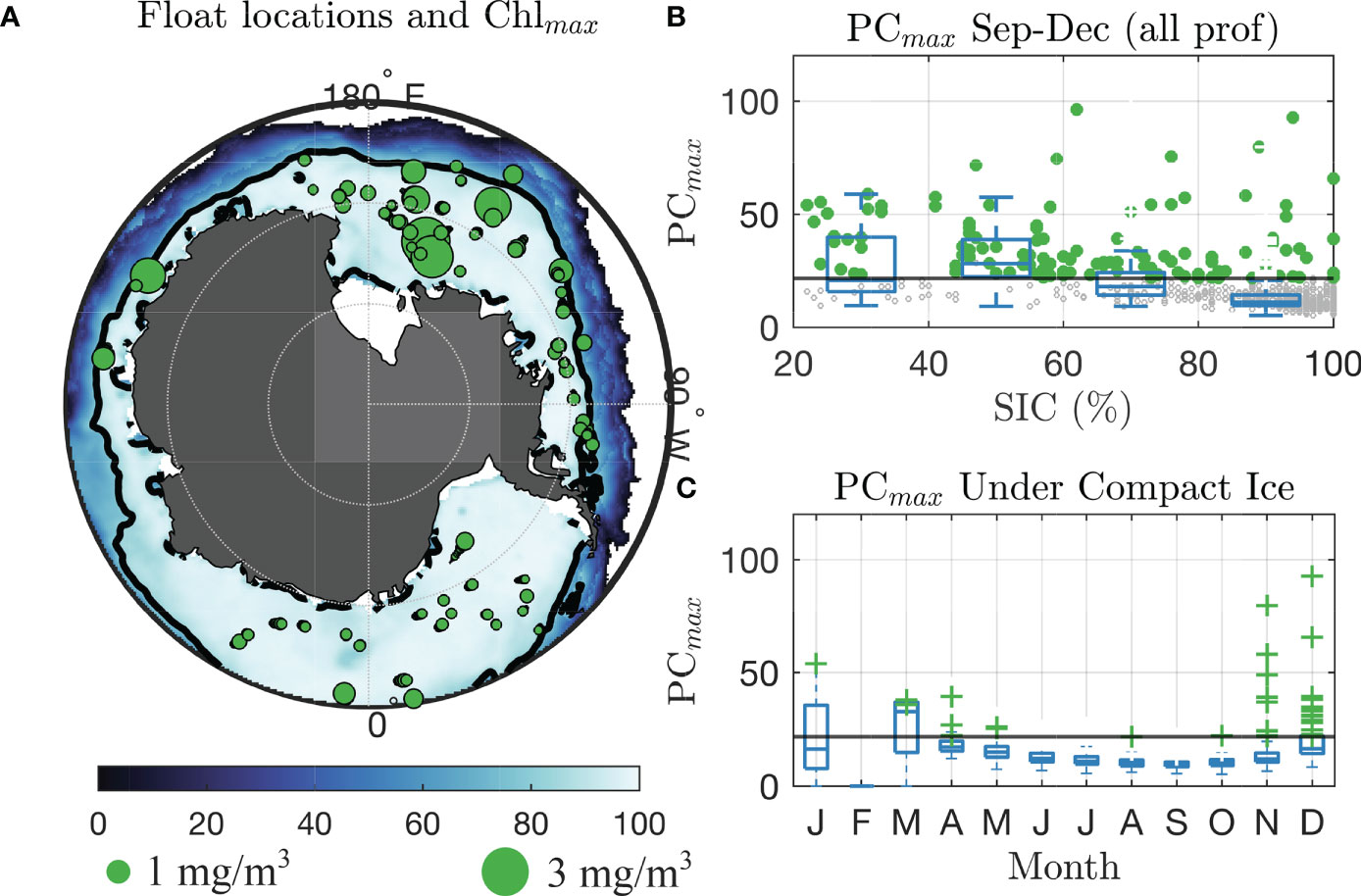
Figure 1 Chlorophyll-a and phytoplankton carbon recorded under compact sea ice by BGC-Argo floats. (A) Climatological sea ice coverage in September–November, 2014–2020. Black line shows 80% concentration contour. Green circles are locations of under-ice Argo float profiles under compact sea ice after October 1, with sizes scaled with value of Chl_max. Green dots outside of map shows sizes corresponding to 1.0 and 3.0 mg/m³. (B) Box plot of PC_max for all BGC-Argo measurements under sea ice, indexed by sea ice concentration. Whiskers extend boxes ±3 standard deviations from the mean in each month, and the vertical blue line is the ensemble median. Crosses show values identified as “UIBs.” The black line is the PC_max bloom threshold. (C) Same as (B), but for PC_max recorded under compact sea ice (concentration >80%) only, indexed by month.

In general, SIC is negatively associated with biomass across all observed data. We plot (gray hashes) values of PC_max for the 731 under-ice profiles from October to January, as a function of local sea ice concentration in Figure 1B. We include box plots in each 20% bin of SIC to illustrate the declining PC_max values with increasing SIC. Measurements meeting the criteria for a UIB are green circles. A total of 119 (16.3%) of under-ice profiles met the criteria for a UIB. Of these, 17/37 (46%) had SIC from 20% to 40%, 39/52 (75%) for SIC from 40% to 60%, 33/95 (35%) for SIC from 60% to 80%, and 30/547 (5.5%) for SIC from 80% to 100% (compact ice). This reinforces the existing understanding that light limitation is key for controlling phytoplankton growth and that ice-edge blooms are ubiquitous. Yet, as we show, phytoplankton biomass is frequently increasing or blooming before the sea ice concentration declines.

Phytoplankton biomass under compact ice increases with increasing solar irradiance. Box plots of PC_max in each month are given in Figure 1C for all under-compact-ice profiles, and we see most “UIB” profiles occurring in November and December. Median PC_max under compact ice ranged from 10.17 mg/m³ (n = 275) in August to a high of 16.4 mg/m³in December (n = 80). The number of UIB profiles was just 1 of 1,269 (0.1%) of profiles measured from June to September, 1 out of 267 (0.4%) of profiles in October, 11 out of 197 (5.6%) of profiles in November, and 18 out of 81 (22.2%) of profiles in December–February. Thus, of all segmented profiles, we find a total of 31 that attained values we deem representative of a UIB in spring–summer. Those profiles had an average PC_max of 35.6 mg/m³ and an average Chl_max of 1.13 mg/m³. We find seven profiles meeting the UIB thresholds in late fall (March–May), which we term “freezeover” profiles, as they are the first under-compact-ice profiles taken by these floats in a given year. They likely derive from sea ice freezing over an existing region of elevated biomass. These seven profiles have a mean Chl_max of 0.39 and a mean PC_max of 27.0, lower than the late spring under-ice valueswe determine to be UIBs.

A majority (68/77, or 88%) of Argo measurements recorded “elevated” photosynthetic biomass when profiling under compact sea ice in late spring–summer, illustrating the fact that photosynthesis is occurring before the seasonal retreat of the sea ice edge. Further, a significant fraction (20/77, or 26%) of the floats reported levels of Chl_max and PC_max that met the adopted criteria for a bloom. We note seven “freeze-over” events, each recording UIB levels of Chl_max and PC_max on their first under-compact-ice profile of the year. In four cases, the float continued to profile under compact ice throughout winter and into spring.

Of the 20 UIB measurements which occur in the spring and summer, six included at least two successive profiles (Argo dives are spaced 10 days apart). These multi-profile events occurred in December 2014 (Argo id 5904183), October–November 2017 (5904860), November 2019 (Argo id 5906000), November–December 2019 (Argo ids 5905635 and 5905997), and December 2020 (Argo id 5905637). The 2014 bloom reported in Briggs et al. (2018) (Argo id 5904184) was also included, as a single profile under compact sea ice at 95% concentration. The estimated locations for each UIB measurement are given in Supporting Figure S4, showing the float location against local sea ice concentration. The six multi-profile events are given as the top two rows, each inside of the sea ice edge. Some of the 14 single-profile events are close to the sea ice edge, demonstrating a need for future work to assess whether these are UIBs or a consequence of advected open-water phytoplankton biomass (see Discussion).

The high under-ice PC and Chl-a measurements recorded here bear an observational signature consistent with light-limited under-ice blooms. In Figure 2A, we plot estimated surface, 25-m average, and mixed-layer average PAR values in the 20 measurements that record a UIB, referenced in time to the first dive recorded as a UIB. While there was high variability in estimated surface PAR values for individual floats (gray lines), there is a noted increase in PAR if averaged across all floats. The recorded values of PC_max for each of these UIB measurements are provided in Figure 2B, showing the rapid increase in phytoplankton carbon that occurs before each event over a multi-week period, underneath compact sea ice.

FIGURE 2

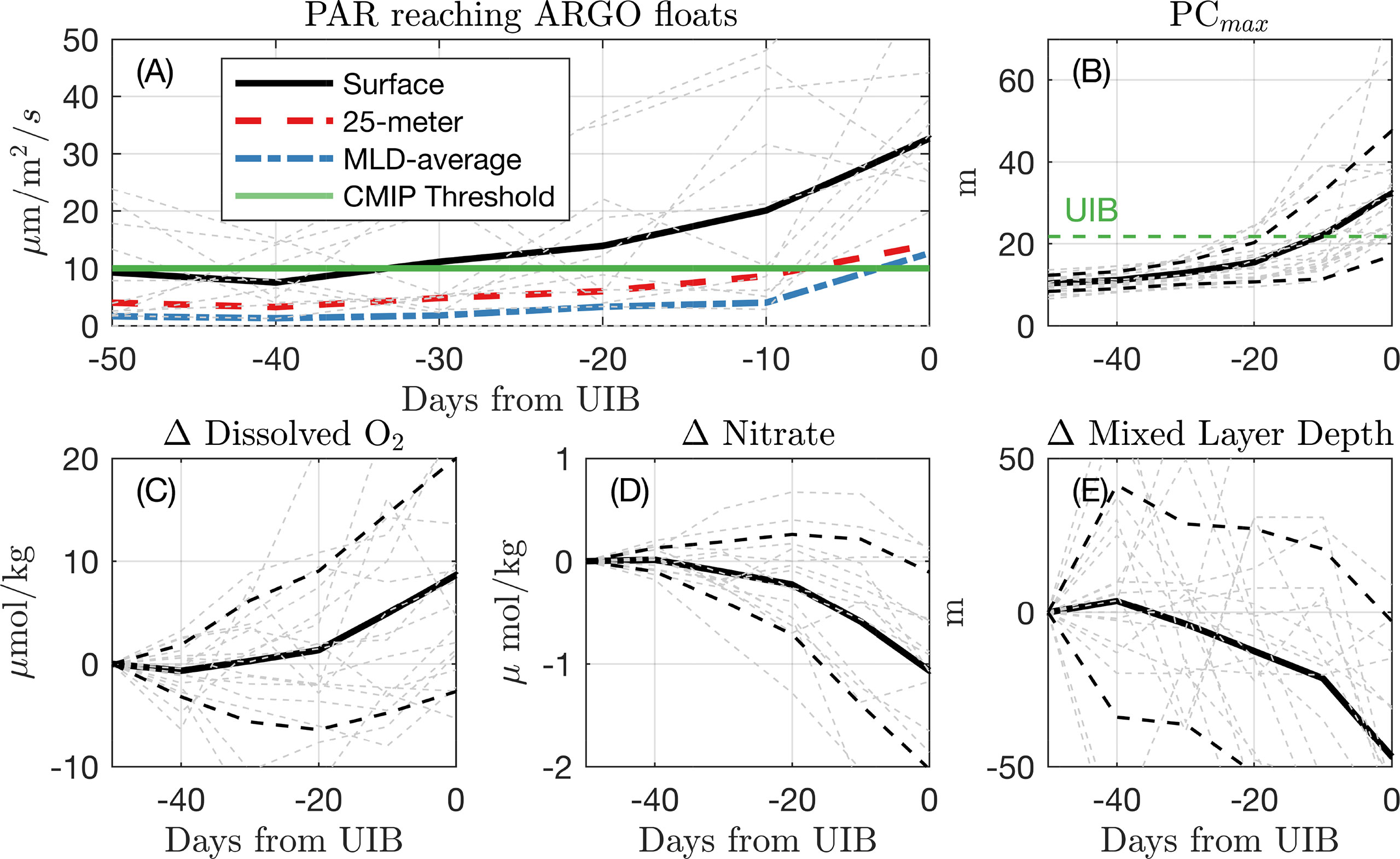
Figure 2 Under-ice conditions preceding UIBs. (A) Averaged estimated PAR for each of the 12 measured “UIBs” for the first profile identified as a UIB and the five preceding under-ice profiles. The black line is the average surface PAR. The red dash line is the average PAR over top 25 m. The blue dot–dash line is PAR averaged over Argo-measured mixed layer depth. The green line indicates the PAR threshold used to define UIBs in CMIP6 data. (B) (C) Change in dissolved oxygen at depth of Chl$_{max}$, relative to the value recorded 50 days (5 dives) preceding the first UIB measurement. (D–E), same as (C) for (D) nitrate at depth of Chl$_{max}$, and (E) mixed layer depth. Dashed lines indicate standard deviation of profile measurements.

At the time of the UIB profile, both mixed-layer average PAR and 25-m average PAR crossed a threshold of 10 μmol photons/m²/s (green horizontal line). We adopt this threshold in Climate-model based bounds on bloom prevalence under Antarctic Sea ice when evaluating the likelihood of observing a bloom in model output data. The median irradiance at 25 m for all UIB measurements was 2.7 μmol photons/m²/s, similar to observed compensation irradiance in Arctic waters (Tremblay et al., 2006) and within the range of reported values in the North Atlantic (Siegel et al., 2002).

We also composite dissolved oxygen (Figure 2C), nitrate (Figure 2D), and mixed layer depth (Figure 2E) for the UIB measurements. Because of differing water conditions at each profile location, we plot in (Figures 2C–E) the difference in these measurements from the profile taken 50 days (5 profiling cycles) preceding the UIB measurement and show the mean (solid lines) and standard deviation (dashed lines) of these anomaly values (light dashed lines). The lead-up to a UIB profile is associated with increasing dissolved oxygen (average eltaO₂≈ 8.7 μmol/kg), decreasing nitrate concentration (average ΔN = -1.1 μmol/kg), and declining mixed layer depths (average ΔH=−46.7 m), all covariant with increases in PAR. Light-limited blooms are often associated with such shoaling mixed layers, which keep phytoplankton in the euphotic layer (Sverdrup, 1953). Autotrophy rates are set by light and nutrient status, and decreasing nitrate concentrations in these surface waters would evince biomass accumulation. As phytoplankton grow, autotrophy will initially exceed heterotrophy in the water column, explaining increases in dissolved oxygen at the surface.

Ultimately, while we have taken a bottom-up view, our results may be compatible with several ecological hypotheses including the “disturbance-recovery” hypothesis (Behrenfeld, 2010; Arteaga et al., 2020), as phytoplankton drift initially in deep MLDs, which might act to dilute them from predators and support their biomass accumulation prior to receiving enhanced light levels with shoaling MLDs. However, due to the poor temporal adjacency of float observations, we could not assess phytoplankton accumulation rates needed to test that hypothesis and others (see Discussion).

3 Climate-model based bounds on bloom prevalence under Antarctic Sea ice

The BGC-Argo float data examined above showed numerous elevated phytoplankton biomass events under compact sea ice in the Southern Ocean. We found that 26% of under-ice measurements reach thresholds which we term a “UIB” before the seasonal loss of sea ice, with 88% showing enhanced phytoplankton biomass, all under sea ice with an average concentration of 96%. Several of these measurements recorded a UIB in November, when Antarctic sea ice is still near its seasonal maximum extent. We next examine climate model and remote sensing output to quantify if conditions that support UIBs are widespread across the sea-ice-covered Southern Ocean before sea ice retreat.

3.1 CMIP6 data

Remote sensing technologies presently do not directly measure light or chlorophyll-a beneath sea ice, and most sampling strategies for Southern Ocean photosynthetic communities associated with sea ice focus on in-ice algae communities in coastal regions (Smetacek et al., 1992; Arrigo and Thomas, 2004; McMinn et al., 2010; Cummings et al., 2019). Therefore, we turned to model estimates, using an ensemble of current-generation coupled climate models contributing to the 6th Coupled Model Intercomparison Project (CMIP6). Each center, by the choice of model and parameters governing that model’s behaviors, will provide a different estimate of the light and ocean conditions governing phytoplankton growth under sea ice. This ensemble is then used to provide a best estimate of the mean and intra-model variance of potential under-ice states.

While observations show Antarctic sea ice has been stable or increased in extent over the satellite period (1978-present), CMIP6 models consistently simulate a declining annual-average Antarctic sea-ice cover over this period (Roach et al., 2020). Thus, we did not consider it feasible to examine present-day model estimates of Antarctic sea ice state. Instead, we postulated that associated light conditions under Antarctic sea ice have remained stable, and used data from preindustrial control run simulations (CMIP6 runs titled picontrol) in this analysis. Of the full CMIP6 model dataset, 11 simulations (see Supporting Table S3) submitted the required model output we used here. Our focus is on the phase space of light and sea ice properties, not specific prediction, so we caution that the use of CMIP6 data is in support of BGC-Argo data but may not be directly comparable.

For each CMIP6 model, we defined a climatology of light and sea ice properties using the final 100 years of their respective preindustrial spin-up experiments. In Figure 3, we specifically examined the Community Earth System Model version 2 (CESM2, Danabasoglu et al., 2020; Singh et al., 2020)) model run, as it uses the more recent version of CICE and the Briegleb (1992) δ-Eddington light scheme. A similar output from CESM2 was analyzed to evaluate the potential for Arctic UIBs in (Ardyna et al., 2020).

We define an area as “permitting” an under-ice bloom if it meets three criteria:

Compact sea ice: Local sea ice concentration exceeds 80% (following World Meteorological Organization (2014)).

An illuminated upper ocean: Average PAR in the top 25 m of the ocean exceeds 10 μmol photons/m²/s over a 10-day period (following Figure 2)

A stable or stratifying surface mixed layer: Sea ice is not refreezing and the upper ocean is non-convecting (following Lowry et al. (2018)).

To quantify the amount of upper-ocean PAR available under the ice, as in Section 2, we estimated PAR at depth H, $\overline{E}(H)$, as

$\begin{array}{ll}\overline{E}=\frac{E_0}{\kappa H}[1-\exp (-\kappa H)].& (2)\end{array}$

CMIP6 models typically store and output full-spectrum solar forcing to the upper ocean, but not PAR. We therefore had to convert full-spectrum solar irradiance to PAR using a factor of 1.9975 μmol photons/J (Yu et al., 2015; Matthes et al., 2019). We assumed positive photosynthesis (gains outweigh losses) occurred when the average PAR over a 25-m deep water column exceeded the threshold value of 10 μmol photons/m²/s established in Section 2 ice and Figure 2A. This value is approximately twice the threshold of integrated daily irradiance of 4.8 μmol photons/m²/s considered to initiate a phytoplankton bloom in other oceans (Letelier et al., 2004; Boss and Behrenfeld, 2010; Oziel et al., 2019), and higher than the levels found to initiate growth in the Southern Ocean (Arteaga et al., 2020; Hague and Vichi, 2021). Note that the surface irradiance in CMIP6 model output is the flux to the ocean surface, and therefore accounts for light penetration through the sea ice itself, unlike our approach in Section 2.

We also include information about the termination of upper-ocean convection. Under-ice blooms are less likely to occur when active convection extends below the euphotic zone, such as when leads are actively refreezing with the ocean at its freezing point (Lowry et al., 2018). The requirement that the upper ocean is non-convecting is similar to the “turbulent shutdown” theory used to explain midlatitude phytoplankton blooms (Taylor and Ferrari, 2011). GCMs used here are too coarse to resolve the complex boundary layer dynamics that result from surface melt processes of sea ice (Holland, 2003; Horvat et al., 2016; Pellichero et al., 2017), and thus, they are not suited for determining the convective state of the upper ocean in the presence of sea ice leads. Instead, we considered the ocean to be non-convecting if sea ice was melting at its base, which would lead to stratification of the upper ocean, consistent with Argo observations of high negative covariance between a shoaling MLD and increasing phytoplankton biomass under ice (Bisson and Cael, 2021).

In practice, simply non-zero basal melting does not restrict the location of UIBs as small monthly averaged basal melt rates occur whenever sea ice is present. We set a positive threshold for the sea ice basal melt rate $\dot{h}$, which we expressed as anequivalent heat flux of $Q={\rho }_i{L}_f\dot{h}$, with the sea ice density of ρ_i = 920 kg/m3 and the latent heat of fusion of L_f=3.34×10⁻⁵ J/kg. As a result, Q is required to exceed 5 W/m2 for an approximate basal melt rate of $\dot{h}=5$ cm/month. While turbulent vertical mixing related to sea ice motion can have a significant impact on local circulation, it does not typically extend beyond several meters in the ocean (Smith and Thomson, 2019; Brenner et al., 2021) and therefore likely does not impact convection at the depths of Chl_max considered here.

3.2 ICESat-2 data

We also approximated the light field under sea ice using new measurements with the ICESat-2 (IS2) laser altimeter. We utilized the L3A along-track sea ice type product (ATL07, Kwok et al. (2019)) derived from Level 2A ATL03 photon heights (Neumann et al., 2019). Sea ice types are determined using an empirical decision tree, which identifies whether a given segment is sea ice or water. We developed an estimate of SIC, which we term the linear ice fraction (LIF), c^* , as the ratio of total ice segment length to total segment length. The LIF is related to the SIC, which is ordinarily defined over a two-dimensional region. Given the random orientation of crack and open water features relative to frequent satellite tracks, many repeated 1D measurements can approximate a 2D field when sampled sufficiently. In Horvat et al. (2020a), we found that global sea ice area metrics derived from passive microwave (PM) satellites were well-approximated by this method in regions where IS2 records at least 1,000 individual segments per month. We adopted this same threshold in this study to define c^* . An advantage of using ICESat-2 segments instead of PM is that ICESat-2 is capable of resolving small cracks and leads that are difficult to observe in PM estimates of local SIC, particularly in summer (Kwok, 2002; Notz et al., 2013; Kern et al., 2020), and that are important for allowing PAR to reach the upper ocean.

From a gridded monthly dataset of

c^*, we estimated the total shortwave irradiance, E0 (

∼ 300–3,000 nm, units W/m2), reaching the upper ocean, E0 (averaged monthly),

$\begin{array}{ll}{E}_0=SW(1-c^{*})(1-{\alpha }_{oc})& (3)\end{array}$

where α_oc=0.06 is the open water albedo and SW is the downwelling solar irradiance (units W/m2) at the surface from [88]. This shortwave irradiance is then converted to a PAR (400–700 nm) estimate as in the CMIP6 model data. This model assumes that no light passes through the sea ice cover and that the only light available in ice-covered regions enters the ocean in the open water areas. For this reason, we consider ICESat-2-derived downwelling irradiances to be conservative. The present-day climatology of E₀ presented in Figure 3 was derived from IS2 data spanning the period from January 2019 to December 2020.

FIGURE 3

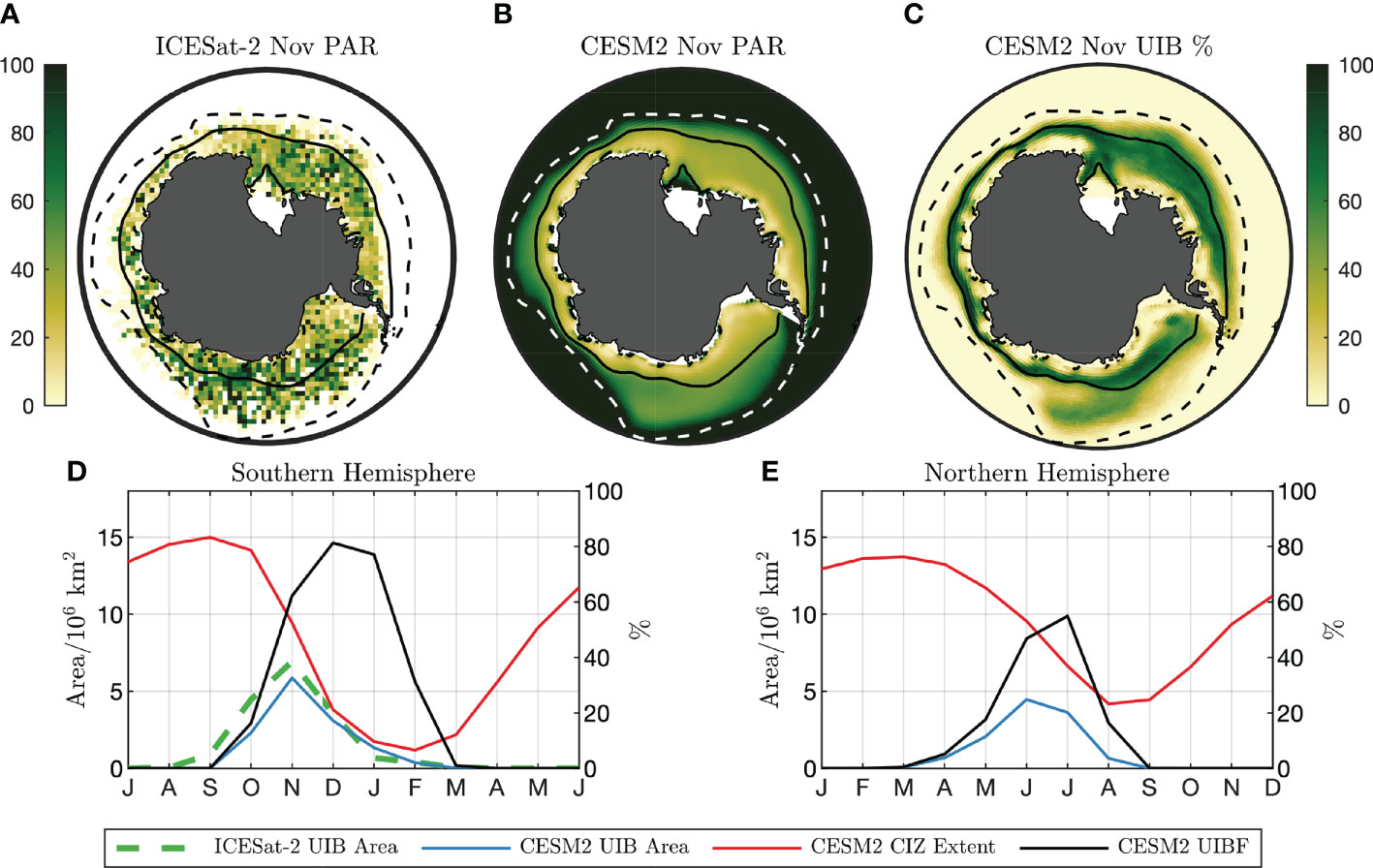
Figure 3 Light field and UIB potential under Southern Ocean sea ice (A) 2018–2020 November surface PAR (μmol photons/m²/s) estimate from ICESat-2. (B) CESM2 climatological PAR from preindustrial simulation. Solid lines in (A, B) are CESM2 climatological CIZ (concentration above 80%). Dashed lines are climatological SIE (concentration above 15%). (C) CESM2 November UIB%. (D, left axis) Seasonal cycle of CESM2 (red) CIZ extent and (blue) UIB extent. The dashed green line is the UIB area from ICESat-2. (D, right axis) CESM2 UIBF. (E) As in (D), but for the Northern Hemisphere. Axes in (D) and (E) are offset by 6 months.

3.3 Model estimates of UIB-permitting areas

In Figure 3A, we show IS2-derived average ocean surface PAR values in the Southern Ocean in November, assuming that no PAR reaches the upper ocean directly through sea ice. A solid line outlines the compact sea ice zone (CIZ, SIC >80%) defined using the NSIDC-CDR SIC product (Meier et al., 2021). We also plot the 15% SIC contour, marking the edge of total sea ice extent (SIE). Regions lying inside the SIE contour but outside the CIZ are defined as marginal ice zones (MIZs), which due to the lower albedo of open water receive higher PAR in the surface water layer compared with the CIZ. Figure 3B shows preindustrial November PAR values for the CESM2 climate model, with CIZ and MIZ defined from the CESM2 model climatology. Both IS2 and CESM2 show large areas within the CIZ where ocean surface PAR estimates exceed a “bloom” threshold of 23 μmol photons/m²/s, sufficient for average insolation within the top 25 m to exceed 10 μmol photons/m²/s. These conditions are representative of the mixed-layer PAR conditions observed in the BGC-Argo UIB profiles (Figure 2A). For the IS2 estimate of ocean surface PAR, 6.9 million km² of the November CIZ exceeds the PAR threshold, versus 5.9 million km² for CESM2. Because we do not have coincident ocean and sea ice melt observations at the scale of IS2 observations, IS2 estimates only indicate the presence of light in the upper ocean and may overestimate the area that permits a UIB.

We next considered how frequently an individual grid cell would permit a UIB over time. Looking across a number of years, we next define the UIB percentage by year (UIB%), equal to the percentage of model years where a grid cell meets all three criteria together. The UIB% can be low if a region is not frequently covered by compact sea ice, not only because the light conditions and ocean stratification are not permissive of a bloom. It can be thought of as the likelihood that an observing station will measure a bloom under compact sea ice in a given year. A spatial map of UIB% in November months is given in Figure 3C for CESM2. Areas within the climatological November CIZ (solid line), which has an area of 8.3 million km², permit a UIB 46.4% of the time. Because of year-to-year variability of the CIZ contour, areas outside of the climatological CIZ also have non-zero UIB%. In those areas, the average UIB% is 19.3%.

We accumulated climatological statistics of UIB-permitting regions in Figure 3D, comparing the climatological extent of compact sea ice (red) to the extent of UIB-permitting regions (blue). Large areas support UIBs, peaking at 5.9 million km² of compact ice-covered regions in November. We next define the UIB fraction (UIBF) in each year and the percentage of the CIZ that would permit a UIB. This quantity is examined in Figure 3D (black line, right axis), peaking in November at a UIBF of 77%. By point of comparison, we reproduce Figures 3D as Figure 3E for the Arctic Ocean. Up to 4.3 million km² of the preindustrial Arctic CIZ is permissive to UIBs, repeating the finding in Ardyna et al. (2020) that large regions of the preindustrial Arctic also supported UIBs. The seasonal maximum of Arctic UIB area occurs in June, at the peak of the solar cycle, with a peak UIBF of 52% in July. Generally, in the CESM2 picontrol experiments, we find that UIB-permitting regions in the Antarctic (1) are larger, (2) constitute a larger percentage of the CIZ, and (3) peak earlier in the annual solar cycle (November in the Antarctic versus June in the Arctic) than in the Arctic.

3.4 Southern ocean UIB statistics across CMIP6 models

In Figures 4A, B, we plot the climatological seasonal cycle of Southern Ocean UIB area (A) and UIBF (B) for the 11 CMIP6 models (listed in Supporting Table S3). Across these models, we found a similar seasonal cycle. None of the CMIP6 models show large UIB areas before October, but 10 of 11 reach a maximum UIB area in November. Only the MRI-ESM2 model shows a maximum UIB area in December. Each model has a climatological UIB area exceeding 2.66 million km², with a median of 4.75 million km². In Figure 4C, we show box plots of the annual maximum UIB area in the Antarctic for each of the models (filled), compared with the annual maximum UIB area in the Arctic (unfilled) for the same years. Out of 11 models, eight have median Antarctic UIB areas that exceed Arctic UIB areas.

FIGURE 4

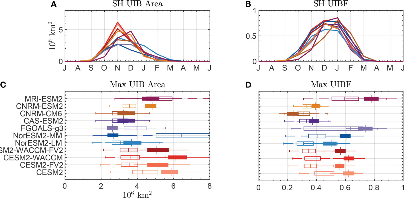
Figure 4 Statistics of bloom-permitting area for CMIP6 models. (A) Seasonal cycle of the UIB-permitting area in the Southern Hemisphere. (B) Seasonal cycle of UIBF. (C) Box plots of the maximum annual UIB area in (filled) the Southern Hemisphere or (unfilled) the Northern Hemisphere. (D) Box plots of UIBF during the month of maximum UIB area. Colors of lines in (A, B) correspond to boxes in (C, D).

We repeat Figures 4A, C in Figures 4B, D for the UIBF, with Figure 4D showing UIBF values during the month where the UIB area is at its maximum (November or December in the Antarctic, June or July in the Arctic). Seasonal cycles of UIBF are similar between models, with most models peaking in December in the Antarctic as the CIZ reduces in extent and ocean surface PAR increases. In 10 of 11 models, a higher fraction of the Antarctic CIZ permits a UIB than of the Arctic CIZ. The average values of UIBF range from 27% to 86% (average 57%) in the Antarctic, compared to 26%–66% in the Arctic (average 37%). Each of the three models, in which Antarctic UIB areas were less than Arctic UIB areas, have higher UIBF in the Antarctic. We hypothesize that the reason for differences in the overall magnitude of Antarctic UIB areas may be caused by differences in model representations of Antarctic and Arctic sea ice instead of disagreements about whether sufficient PAR is available under the compact sea ice in both regions.

3.5 Targeting in situ observations of Antarctic UIBs

Using BGC-Argo float data, we have demonstrated that high phytoplankton biomass events exist under compact sea ice in the Southern Hemisphere, preceding the seasonal loss of sea ice by several months as well as the seasonal maximum downwelling solar irradiance. Examining a series of climate model estimates of upper ocean light and sea ice conditions, we found that under-ice phytoplankton growth would be permitted across a wide fraction of the compact ice-covered Southern Ocean. We also found that areas permitting UIBs make up a larger percentage of compact sea ice zones in the Southern Ocean than the Arctic, with an earlier peak in the seasonal cycle. Further validation will be needed, as the BGC-Argo data are spatially and temporally sparse, and the CMIP6 data rely on parameterizations of light transmission through ice and assumptions about what conditions are necessary to permit a bloom.

To highlight areas of importance for additional in situ observations, we specifically focused on the potential of the Ross Sea region to support UIBs. To define the Ross Sea region, we followed the convention established by the NIWA Ross Sea Trophic Model (Pinkerton et al., 2010), taking the ocean region south of 69 ^∘ S and between 160 ^∘ W and 170 ^∘ E longitude. Because of grid variations, the area of this region can vary between CMIP6 models, but its surface area is approximately 1.5 million km2. We chose this area as it is seasonally ice free, is among the highest-productivity regions of the Southern Ocean, and is known for supporting large ice-algal communities (Lizotte, 2001; Arrigo, 2003).

In Figure 5, we plot UIB% for each of the 11 models during the model period with highest Ross Sea UIB area, which is November in seven models and December in four models. All models have high UIB% in the coastal region near Cape Adare in the Western Ross Sea, which has compact sea ice into January. We marked this region at 72 ^∘ S, 178.5 ^∘ E with a blue square in Figure 5. A box plot of UIB% in this location is given for these 11 models in Figure 5 (bottom right), showing a median UIB% of 62% with a minimum of 40%. Across the CMIP6 models, a mean area of 0.55 million km2 of the Ross Sea is expected to permit UIBs, although the borders of UIB-permitting areas vary by model and range from 0.29 million km2 (MRI-ESM2, 49% of the Ross CIZ) to 0.95 million km2 (NorESM2-LM, 65% of the Ross CIZ), including interannual variability. Independent of modeled sea-ice area coverage, a large fraction of the Ross CIZ permits UIBs in each year in all models. Figure 4 is repeated as Supporting Figure S5 for the Ross Sea region, showing that during the month of highest Ross Sea UIB area, at least 49% of the Ross CIZ permits UIBs in each model, with an average of 60%.

FIGURE 5

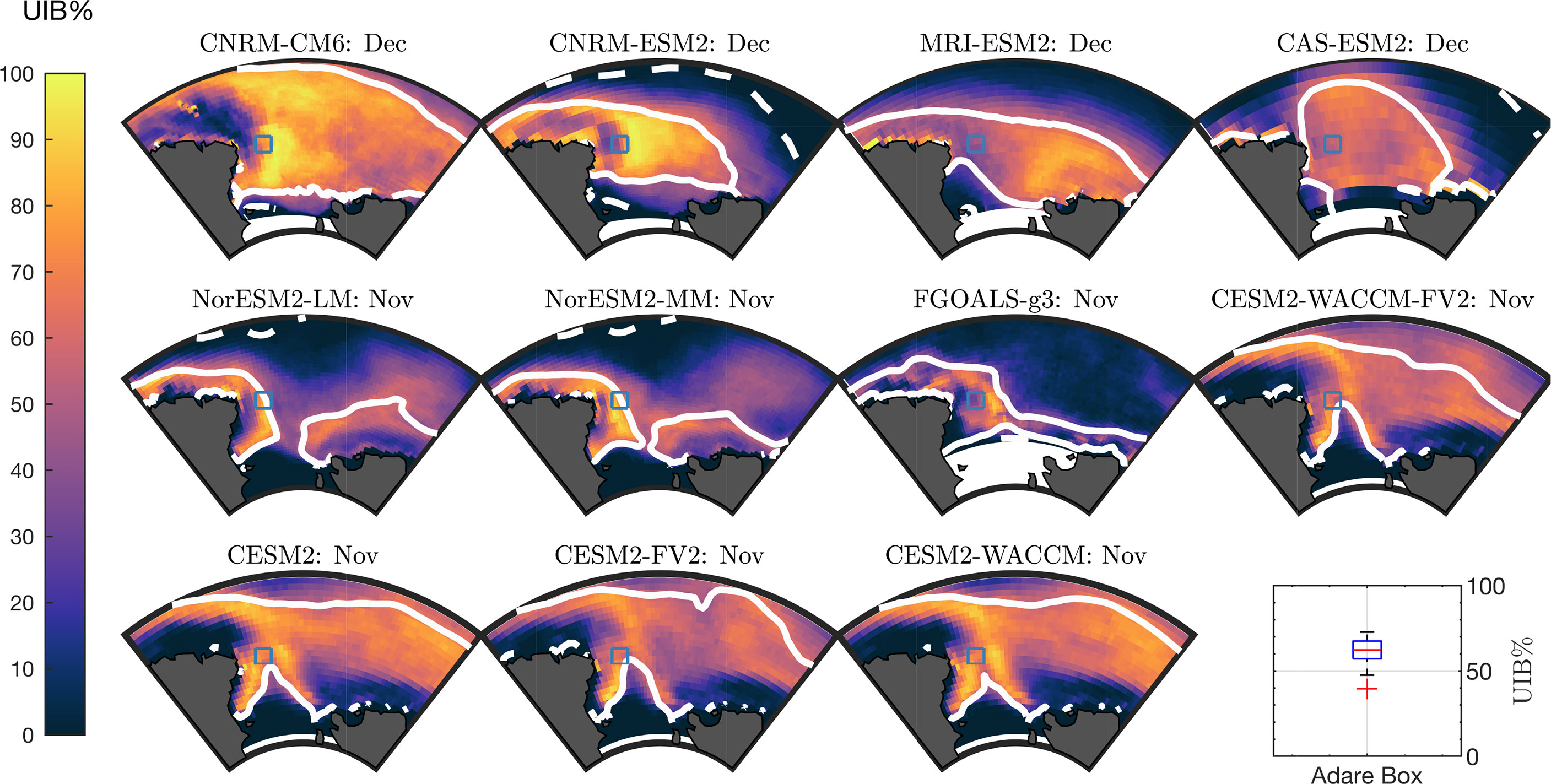
Figure 5 UIB likelihoods in the Ross Sea. Ross Sea UIB% for each model in the month of the maximum UIB area. Solid lines are climatological CIZ. Dashed lines are climatological SIE. Blue square highlights the location of interest at 72°S,178°E. Box plot (bottom right) is of UIB% at square location.

4 Discussion

In this study, we explored the potential for under-ice phytoplankton blooms beneath compact sea ice in the Southern Ocean using model simulations, altimetric measurements of sea ice coverage, and BCG-Argo float data. We showed that 26% of 77 BGC-Argo measurements recorded Chl-a and phytoplankton carbon meeting criteria for UIBs and 88% indicating enhanced under-ice phytoplankton biomass preceding ice retreat. These observations suggest that even for areas with a low open water fraction, incident solar radiation is high enough to promote photosynthetic activity, potentially because the phytoplankton are well adapted to low-light conditions. By evaluating the relationship between under-ice Chl-a and PC to sea ice concentration, we showed that increasing light levels are associated with increasing photosynthetic biomass. Our findings are similar to those in the Arctic, where increased light availability caused by small leads was sufficient to support under-ice blooming (Assmy et al., 2017). Because BGC-Argo floats avoid the surface ocean under ice, and drift with prevailing currents, they may also be underestimating the frequency and magnitude of these events. Thus, data presented here suggest that small regions of open water are sufficient to relax light limitations on under-ice phytoplankton growth in the summertime Southern Ocean.

We have defined a “UIB” in BGC-Argo data in a relative sense, i.e., compared with background values measured in the Southern Ocean under ice (i.e., not relative to the global phytoplankton carbon measurements) (Moore and Abbott, 2000; Haëntjens et al., 2017). This can lead to areas with lower phytoplankton biomass than were, for example, observed in the Arrigo et al. (2010) bloom being recorded as a UIB. Yet, values actually attained in UIB profiles here were not regionally low. For example, observations of an open-water bloom near the West Antarctic Peninsula (Arrigo et al., 2017) average surface Chl-a values ranging from 0.3 to 0.6 mg/m³, as high as 1.1 mg/m³ when only including waters on the West Antarctic Shelf, with substantial spatial variation. Peak Chl_max values at the core of the sampled bloom reached 2.3 mg/m³, but outside of the bloom core, reported values of Chl_max were 1.3 mg/m³ or lower Arrigo et al. (2017).

In contrast, the highest-quality-controlled Chl_max recorded in under-compact-ice measurements was 3.6 mg/m³ taken by float 5904860 on 18 December 2017 under sea ice with a concentration of 91% and with a corresponding PC_max of 38.3 mg/m³. The highest PC_max we analyzed was 92.8mg/m³, recorded by float 5905997 on 5 December 2020 under sea ice with a concentration of 94% and corresponding to a Chl_max of 2.87 mg/m³. The mean Chl_max value for the 20 UIB measurements was 0.96 mg/m³, and the mean PC_max was 36.6 mg/m³. As we noted above, the intermittency and surface avoidance of under-ice BGC Argo floats likely preclude sampling the spatial core of any bloom, and these measurements must necessarily underestimate the peak values observable in any individual event.

We supplemented the PC_max observations with observed nitrate and dissolved oxygen concentrations at the depth of Chl_max and observed mixed-layer depths. Increasing dissolved oxygen concentrations toward the time of peak PC_max together with decreasing nitrate indicate an enhanced phytoplankton biomass accumulation. Our conclusion of increasing phytoplankton (i.e., biomass) concentrations is further supported by the observed high correlation between Chl-a and phytoplankton carbon (Spearman’s R = 0.7, see Supporting Info Figure S1). Ultimately, the highest biomass blooms were in November, occurring before sea ice retreat. We suggest that the November blooms are caused by low zooplankton predation combined with low-light-adapted phytoplankton that are able to grow rapidly as the mixed layer shoals and light availability increases.

Presented ICESat-2 and an ensemble of climate model estimates of sea ice, light, and oceanographic conditions across the compact-ice-covered Southern Ocean also showed that conditions are favorable for under-ice blooms over wide regions, with a median estimated UIB area of 4.75 million km² across the model ensemble. In using ICESat-2 data, we assumed that no light was transmitted through sea ice and all light available for photosynthesis entered the water column in open water regions near compact ice. We find that the month with the largest potential area for permitting under-ice photosynthesis is in November rather than December, where there is more sunlight, a result of both the higher overall sea ice area in November and the fact that solar irradiance is yet high enough to allow for UIBs, as seen in BGC-Argo data. Thus, these findings indicate that even in regions with local sea ice concentrations above 80%, enough open water areas exist to support light-limited phytoplankton growth in the upper Southern Ocean (Hague and Vichi, 2021).

The climate models considered here have interrelated sea ice and light schemes (see Supporting Table S3) and provide estimates of the light conditions in the Southern Ocean. They may not be accurate if systematic biases in the modeled Southern Ocean phase space of light and sea ice properties exist. We adopted a diagnostic criteria for when sufficient light is available to support a bloom, using a fixed PAR threshold in model data based on our observations of UIBs in BGC-Argo data, which is in line with Arctic modeling studies and observations of photoacclimation in key Antarctic phytoplankton species (Arrigo et al., 2010). While some BGC-Argo floats do report PAR values, none of the ice-enabled floats included in this study did. Further observations and modeling of radiative transfer of PAR specifically focused on variable Antarctic sea ice conditions (as in, for example, Horvat et al. (2020b); Katlein et al. (2021)) would help constrain and evaluate PAR levels needed to trigger blooms observed in BGC-Argo data.

4.1 Future directions for observing and contextualizing Antarctic under-ice blooms

The work we presented here raises an important question: if conditions beneath compact sea ice are favorable for supporting UIBs, if Antarctic sea ice coverage and downwelling irradiance have remained largely stable over the past several decades, and if BGC-Argo floats repeatedly observe high levels of phytoplankton biomass, why are there no reported observations of under-ice blooms in the Southern Ocean made during research cruises or recorded by long-term mooring deployments? We suggest two potential answers.

First, the detection of UIBs requires a dedicated effort to collect in situ phytoplankton biomass data under compact sea ice. An analogy can be drawn to the Arctic Ocean, where spring–summer icebreaker research expeditions are more common. UIBs are now thought to have been widespread dating back to at least the 1950s (with an overall area coverage that has doubled since 1970 (Ardyna et al., 2020)). However, these phenomena, which can have some of the highest levels of integrated biomass of any ecological system (Arrigo et al., 2012), were rarely observed before the report of a massive under-ice bloom in the Chukchi Sea in 2011. BGC-Argo floats permit a broader sampling of biological parameters across the Southern Hemisphere using consistent methodologies and calibrations. We did not mine previous ship-based under-ice Chl-a and backscatter data, for example from the BCO-DMO archive, as BGC-Argo floats provide broader and more regular spatial and temporal coverage with consistent instrument calibration. Still, such data and assimilating models like B-SOSE will be a focus of future work to understand whether such events were common in the past.

Second, it is possible that UIBs do not occur as regularly as suggested by models. Out of all measurements, 26% contain profiles meeting our UIB threshold, lower values than observed in the Chukchi bloom Arrigo et al. (2010). This mismatch points toward fruitful future research and observation. It is clear in a wide majority of float measurements (88%) that elevated phytoplankton biomass precedes the retreat of sea ice, and so this discrepancy may be a result of a too-broad temporal sampling of the under-ice ecosystem by Argo floats, a spatial bias in the deployment of floats, or that rapid sea ice loss uncovers productive regions before they can be termed a “bloom.” The modeling we examine here does not consider factors like community growth, iron limitation, viral lysis, or predation by zooplankton. It is simply based on a set of diagnostic criteria using bulk estimates for light transmission and stratification as detailed biogeochemical modeling was beyond the scope of this study, following the perspective of van Oijen (2004), arguing that primary production is primarily light-limited in the summer Southern Ocean. While the BGC-Argo data, as in Arteaga et al. (2020) and Hague and Vichi (2021), confirm that under-ice regions are productive, we caution it is not possible to directly compare geographic estimates of model-predicted conditions with float data because of uneven spatial coverage (Supporting Info Figure S3).

As after the observation of a UIB in the Chukchi Sea, more work may be necessary to ascertain the provenance of the 20 high-PC and high-Chl-a measurements seen here, requiring detailed oceanographic and biological modeling. In Supporting Figure S4, we show the location of float when recording a UIB, along with local SIC measured on the day of the highest PC_max measurement, along with lat/lon data for UIB profiles taken preceding this maximum. Several UIB profiles were recorded near the sea ice edge. Because of uncertainty in prescribing a specific lat/lon coordinate to under-ice profiles, the potential influence of ice-free waters for UIB profiles recorded near the ice edge will be important to address in future work (see Discussion). Those UIB measurements with more than one consecutive profile meeting the specified thresholds were all significantly inside the sea ice edge at the time the UIBs were recorded and likely not the result of ice-edge advection of Chl-a. Investigation of combined data/modeling sources, like the biogeochemical Southern Ocean State Estimate (SOSE) (Verdy and Mazloff, 2017), may provide a pathway toward observation-model comparison and the estimation of pan-Antarctic UIB extent.

5 Summary

Our presented results, drawn from observations and simulations, suggest underexplored ecological variability beneath Southern Ocean sea ice, and several million square kilometers of the ice-covered Southern Ocean potentially permitting phytoplankton blooms before seasonal ice retreat. We paid special attention to the frequently visited Ross Sea region and suggest detailed measurements of physical and biogeochemical variables to study under-ice phytoplankton bloom phenology, magnitude, and community composition, and to compare those with known bloom dynamics in the Arctic Ocean (Chase et al., 2020). Sampling during the sea ice-covered season will be challenging, especially as remote sensing technologies presently cannot measure Chl-a under sea ice. Continued targeted deployment of remotely operated and autonomous platforms (Arteaga et al., 2020; Hague and Vichi, 2021) to measure under-ice light availability and bio-optical parameters, in combination with ICESat-2 measurements to remotely sense particulate backscatter (Lu et al., 2020) in open water areas within sea-ice-covered regions, can be complementary to ship-based sampling.

Data availability statement

Code for processing data and producing Antarctic under-ice light fields and UIB-permitting criteria is publicly available on github at https://github.com/chhorvat/Antarctic-Light/, with releases archived in the Zenodo repository (Horvat et al., 2021).

Author contributions

CH and SS designed the study. CH performed the data analysis and prepared the manuscript. KB processed and analyzed presented BGC-Argo data. All authors assisted with study design and manuscript writing. All authors contributed to the article and approved the submitted version.

Funding

CH was supported by NASA grant 80NSSC20K0959 and by Schmidt Futures — a philanthropic initiative that seeks to improve societal outcomes through the development of emerging science and technologies. KB was supported by NASA grant 80NSSC20K0970 and thanks Tanya Maurer at MBARI for help with BGC-Argo under-ice identification. LM was supported by funding from the Weston Foundation.

Acknowledgments

We acknowledge the World Climate Research Programme, which, through its Working Group on Coupled Modelling, coordinated and promoted CMIP6. We thank the climate modeling groups for producing and making available their model output, the Earth System Grid Federation (ESGF) for archiving the data and providing access, and the multiple funding agencies who support CMIP6 and ESGF. These Argo data were collected and made freely available by the International Argo Program and the national programs that contribute to it. (https://argo.ucsd.edu, https://www.ocean-ops.org). The Argo Program is part of the Global Ocean Observing System. CH thanks the National Institute of Water and Atmospheric Research in Wellington, NZ, for their hospitality during parts of this work.

Conflict of interest

The authors declare that the research was conducted in the absence of any commercial or financial relationships that could be construed as a potential conflict of interest.

Publisher’s note

All claims expressed in this article are solely those of the authors and do not necessarily represent those of their affiliated organizations, or those of the publisher, the editors and the reviewers. Any product that may be evaluated in this article, or claim that may be made by its manufacturer, is not guaranteed or endorsed by the publisher.

Supplementary material

The Supplementary Material for this article can be found online at: https://www.frontiersin.org/articles/10.3389/fmars.2022.942799/full#supplementary-material

References

Apollonio S. (1959). Hydrobiological measurements on IGY Drifting Station Bravo. Natl. Acad. Sci. IGY Bull 27, 16–19. doi: 10.13155/40879

CrossRef Full Text | Google Scholar

Ardyna M., Babin M., Gosselin M., Devred E., Bélanger S., Matsuoka A., et al. (2013). Parameterization of vertical chlorophyll a in the Arctic ocean: Impact of the subsurface chlorophyll maximum on regional, seasonal, and annual primary production estimates. Biogeosciences 10, 4383–4404. doi: 10.5194/bg-10-4383-2013

CrossRef Full Text | Google Scholar

Ardyna M., Mundy C. J., Mayot N., Matthes L. C., Oziel L., Horvat C., et al. (2020). Under-ice phytoplankton blooms: Shedding light on the “Invisible”. Part of Arctic primary production. Front. Mar. Sci. 7. doi: 10.3389/fmars.2020.608032

CrossRef Full Text | Google Scholar

Arndt S., Meiners K. M., Ricker R., Krumpen T., Katlein C., Nicolaus M. (2017). Influence of snow depth and surface flooding on light transmission through Antarctic pack ice. J. Geophys. Res.: Oceans 122, 2108–2119. doi: 10.1002/2016JC012325

CrossRef Full Text | Google Scholar

Arrigo K. R. (2003). Physical control of chlorophyll a, POC, and TPN distributions in the pack ice of the Ross Sea, Antarctica. J. Geophys. Res. 108, 3316. doi: 10.1029/2001JC001138

CrossRef Full Text | Google Scholar

Arrigo K. R., Mills M. M., Kropuenske L. R., Van Dijken G. L., Alderkamp A. C., Robinson D. H. (2010). Photophysiology in two major southern ocean phytoplankton taxa: Photosynthesis and growth of phaeocystis antarctica and fragilariopsis cylindrus under different irradiance levels. Integr. Comp. Biol. 50, 950–966. doi: 10.1093/icb/icq021

PubMed Abstract | CrossRef Full Text | Google Scholar

Arrigo K. R., Perovich D. K., Pickart R. S., Brown Z. W., van Dijken G. L., Lowry K. E., et al. (2012). Massive phytoplankton blooms under Arctic Sea ice. Science 336, 1408. doi: 10.1126/science.1215065

PubMed Abstract | CrossRef Full Text | Google Scholar

Arrigo K. R., Perovich D. K., Pickart R. S., Brown Z. W., van Dijken G. L., Lowry K. E., et al. (2014). Phytoplankton blooms beneath the sea ice in the chukchi sea. Deep-Sea Res. Part II: Topical Stud. Oceanog. 105, 1–16. doi: 10.1016/j.dsr2.2014.03.018

CrossRef Full Text | Google Scholar

Arrigo K. R., Thomas D. N. (2004). Large Scale importance of sea ice biology in the southern ocean. Antarct. Sci. 16, 471–486. doi: 10.1017/S0954102004002263

CrossRef Full Text | Google Scholar

Arrigo K. R., van Dijken G. L., Alderkamp A., Erickson Z. K., Lewis K. M., Lowry K. E., et al. (2017). Early spring phytoplankton dynamics in the Western Antarctic peninsula. J. Geophys. Res.: Oceans 122, 9350–9369. doi: 10.1002/2017JC013281

CrossRef Full Text | Google Scholar

Arteaga L. A., Boss E., Behrenfeld M. J., Westberry T. K., Sarmiento J. L. (2020). Seasonal modulation of phytoplankton biomass in the southern ocean. Nat. Commun. 11, 5364. doi: 10.1038/s41467-020-19157-2

PubMed Abstract | CrossRef Full Text | Google Scholar

Assmy P., Fernández-Méndez M., Duarte P., Meyer A., Randelhoff A., Mundy C. J., et al. (2017). Leads in Arctic pack ice enable early phytoplankton blooms below snow-covered sea ice. Sci. Rep. 7, 40850. doi: 10.1038/srep40850

PubMed Abstract | CrossRef Full Text | Google Scholar

Behrenfeld M. J. (2010). Abandoning sverdrup’s critical depth hypothesis on phytoplankton blooms. Ecology 91, 977–989. doi: 10.1890/09-1207.1

PubMed Abstract | CrossRef Full Text | Google Scholar

Bisson K. M., Boss E., Werdell P. J., Ibrahim A., Behrenfeld M. J. (2021). Particulate backscattering in the global ocean: A comparison of independent assessments. Geophys. Res. Lett. 48. doi: 10.1029/2020GL090909

CrossRef Full Text | Google Scholar

Bisson K. M., Boss E., Westberry T. K., Behrenfeld M. J. (2019). Evaluating satellite estimates of particulate backscatter in the global open ocean using autonomous profiling floats. Optics Express 27, 30191. doi: 10.1364/OE.27.030191

PubMed Abstract | CrossRef Full Text | Google Scholar

Bisson K. M., Cael B. B. (2021). How are under ice phytoplankton related to sea ice in the southern ocean? Geophys. Res. Lett. 48, 1–14. doi: 10.1029/2021GL095051

CrossRef Full Text | Google Scholar

Boles E., Provost C., Garçon V., Bertosio C., Athanase M., Koenig Z., et al. (2020). Under-ice phytoplankton blooms in the central Arctic ocean: Insights from the first biogeochemical IAOOS platform drift in 2017. J. Geophys. Res.: Oceans 125, 6069–6079. doi: 10.1029/2019JC015608

CrossRef Full Text | Google Scholar

Boss E., Behrenfeld M. (2010). In situ evaluation of the initiation of the north Atlantic phytoplankton bloom. Geophys. Res. Lett. 37, 1–5. doi: 10.1029/2010GL044174

CrossRef Full Text | Google Scholar

Brandt R. E., Warren S. G., Worby A. P., Grenfell T. C. (2005). Surface albedo of the Antarctic Sea ice zone. J. Climate 18, 3606–3622. doi: 10.1175/JCLI3489.1

CrossRef Full Text | Google Scholar

Brenner S., Rainville L., Thomson J., Cole S., Lee C. (2021). Comparing observations and parameterizations of ice-ocean drag through an annual cycle across the Beaufort Sea. J. Geophys. Res.: Oceans 126. doi: 10.1029/2020JC016977

CrossRef Full Text | Google Scholar

Briegleb B. P. (1992). Delta Eddington approximation for solar radiation in the NCAR community climate model. J. Geophys. Res. 97, 7603–7612. doi: 10.1029/92JD00291

CrossRef Full Text | Google Scholar

Briggs E. M., Martz T. R., Talley L. D., Mazloff M. R., Johnson K. S. (2018). Physical and biological drivers of biogeochemical tracers within the seasonal Sea ice zone of the southern ocean from profiling floats. J. Geophys. Res.: Oceans 123, 746–758. doi: 10.1002/2017JC012846

CrossRef Full Text | Google Scholar

Brown Z. W., Lowry K. E., Palmer M. A., van Dijken G. L., Mills M. M., Pickart R. S., et al. (2015). Characterizing the subsurface chlorophyll a maximum in the chukchi Sea and Canada basin. Deep-Sea Res. Part II: Topical Stud. Oceanog. 118, 88–104. doi: 10.1016/j.dsr2.2015.02.010

CrossRef Full Text | Google Scholar

Chase A. P., Kramer S. J., Haëntjens N., Boss E. S., Karp-Boss L., Edmondson M., et al. (2020). Evaluation of diagnostic pigments to estimate phytoplankton size classes. Limnol. Oceanog.: Methods. 18 (10), 570–584. doi: 10.1002/lom3.10385

CrossRef Full Text | Google Scholar

Claustre H., Claustre H., Claustre H., Claustre H., Claustre H., Claustre H., et al. (2010). Bio-optical profiling floats as new observational tools for biogeochemical and ecosystem studies: Potential synergies with ocean color remote sensing. In Proc. OceanObs’09: Sustain. Ocean Observations Inf. Soc. (European Space Agency) 1, 177–183. doi: 10.5270/OceanObs09.cwp.17

CrossRef Full Text | Google Scholar

Claustre H., Johnson K. S., Takeshita Y. (2020). Observing the global ocean with biogeochemical-argo. Annu. Rev. Mar. Sci. 12, 23–48. doi: 10.1146/annurev-marine-010419-010956

CrossRef Full Text | Google Scholar

Comiso J. C., McClain C. R., Sullivan C. W., Ryan J. P., Leonard C. L. (1993). Coastal zone color scanner pigment concentrations in the southern ocean and relationships to geophysical surface features. J. Geophys. Res.: Oceans 98, 2419–2451. doi: 10.1029/92JC02505

CrossRef Full Text | Google Scholar

Cuevas C. A., Maffezzoli N., Corella J. P., Spolaor A., Vallelonga P., Kjær H. A., et al. (2018). Rapid increase in atmospheric iodine levels in the north Atlantic since the mid-20th century. Nat. Commun. 9, 1452. doi: 10.1038/s41467-018-03756-1

PubMed Abstract | CrossRef Full Text | Google Scholar

Cummings V. J., Barr N. G., Budd R. G., Marriott P. M., Safi K. A., Lohrer A. M. (2019). In situ response of Antarctic under-ice primary producers to experimentally altered pH. Sci. Rep. 9, 6069. doi: 10.1038/s41598-019-42329-0

PubMed Abstract | CrossRef Full Text | Google Scholar

Danabasoglu G., Lamarque J. F., Bacmeister J., Bailey D. A., DuVivier A. K., Edwards J., et al. (2020). The community earth system model version 2 (CESM2). J. Adv. Modeling Earth Syst. 12, 1–35. doi: 10.1029/2019MS001916

CrossRef Full Text | Google Scholar

Dong S., Sprintall J., Gille S. T., Talley L. (2008). Southern ocean mixed-layer depth from argo float profiles. J. Geophys. Res.: Oceans 113, 1–12. doi: 10.1029/2006JC004051

CrossRef Full Text | Google Scholar

Graff J. R., Westberry T. K., Milligan A. J., Brown M. B., Dall’Olmo G., van Dongen-Vogels V., et al. (2015). Analytical phytoplankton carbon measurements spanning diverse ecosystems. Deep Sea Res. Part I: Oceanog. Res. Papers 102, 16–25. doi: 10.1016/j.dsr.2015.04.006

CrossRef Full Text | Google Scholar

Haëntjens N., Boss E., Talley L. D. (2017). Revisiting ocean color algorithms for chlorophyll-a and particulate organic carbon in the southern ocean using biogeochemical floats. J. Geophys. Res.: Oceans 122, 6583–6593. doi: 10.1002/2017JC012844

CrossRef Full Text | Google Scholar

Haëntjens N., Della Penna A., Briggs N., Karp-Boss L., Gaube P., Claustre H., et al. (2020). Detecting mesopelagic organisms using biogeochemical-argo floats. Geophys. Res. Lett. 47, e2019GL086088. doi: 10.1029/2019GL086088

PubMed Abstract | CrossRef Full Text | Google Scholar

Hague M., Vichi M. (2021). Southern ocean biogeochemical argo detect under-ice phytoplankton growth before sea ice retreat. Biogeosciences 18, 25–38. doi: 10.5194/bg-18-25-2021

CrossRef Full Text | Google Scholar

Hergert W., Wriedt T. eds. (2012). The mie theory: basics and applications (Springer) 169.

Google Scholar

Holland M. M. (2003). An improved single-column model representation of ocean mixing associated with summertime leads: Results from a SHEBA case study. J. Geophys. Res. 108, 3107. doi: 10.1029/2002JC001557

CrossRef Full Text | Google Scholar

Horvat C. (2022). Floes, the marginal ice zone and coupled wave-sea-ice feedbacks. Philos. Trans. R. Soc. A: Math. Phys. Eng. Sci. 380, 20210252. doi: 10.1098/rsta.2021.0252

CrossRef Full Text | Google Scholar

Horvat C., Blanchard-Wrigglesworth E., Petty A. (2020a). Observing waves in sea ice with ICESat-2. Geophys. Res. Lett. 47.10 (2020), e2020GL087629. doi: 10.1029/2020GL087629

CrossRef Full Text | Google Scholar

Horvat C., Flocco D., Rees Jones D. W., Roach L., Golden K. M. (2020b). The effect of melt pond geometry on the distribution of solar energy under first-year Sea ice. Geophys. Res. Lett. 47, e2019GL085956. doi: 10.1029/2019GL085956

CrossRef Full Text | Google Scholar

Horvat C., Jones D. R., Iams S., Schroeder D., Flocco D., Feltham D. (2017). The frequency and extent of sub-ice phytoplankton blooms in the Arctic ocean. Sci. Adv. 3, e1601191. doi: 10.1126/sciadv.1601191

PubMed Abstract | CrossRef Full Text | Google Scholar

Horvat C., Seabrook S., Cristi A., Matthes L., Bisson K. (2021). Code for: The case for phytoplankton blooms under Antarctic Sea ice. Tech. Rep. doi: 10.5281/zenodo.4579199

CrossRef Full Text | Google Scholar

Horvat C., Tziperman E., Campin J.-M. (2016). Interaction of sea ice floe size, ocean eddies, and sea ice melting. Geophys. Res. Lett. 43, 8083–8090. doi: 10.1002/2016GL069742

CrossRef Full Text | Google Scholar

Johnson K. S., Plant J. N., Coletti L. J., Jannasch H. W., Sakamoto C. M., Riser S. C., et al. (2017). Biogeochemical sensor performance in the SOCCOM profiling float array. J. Geophys. Res.: Oceans 122, 6416–6436. doi: 10.1002/2017JC012838

CrossRef Full Text | Google Scholar

Katlein C., Valcic L., Lambert-Girard S., Hoppmann M. (2021). New insights into radiative transfer within sea ice derived from autonomous optical propagation measurements. Cryosphere 15, 183–198. doi: 10.5194/tc-15-183-2021

CrossRef Full Text | Google Scholar

Kern S., Lavergne T., Notz D., Pedersen L. T., Tonboe R. (2020). Satellite passive microwave sea-ice concentration data set inter-comparison for Arctic summer conditions. Cryosphere 14, 2469–2493. doi: 10.5194/tc-14-2469-2020

CrossRef Full Text | Google Scholar

Klatt O., Boebel O., Fahrbach E. (2007). A profiling float’s sense of ice. J. Atmos. Oceanic Technol. 24, 1301–1308. doi: 10.1175/JTECH2026.1

CrossRef Full Text | Google Scholar

Kwok R. (2002). Sea Ice concentration estimates from satellite passive microwave radiometry and openings from SAR ice motion. Geophys. Res. Lett. 29, 25–1–25–4. doi: 10.1029/2002GL014787

CrossRef Full Text | Google Scholar

Kwok R., Cunningham G., Markus T., Hancock D., Morison J., Palm S. P., et al. (2019). ATLAS/ICESat-2 L3A Sea ice height, version 1. boulder, Colorado USA (Colorado USA: Tech. Rep. May, NSIDC, Boulder). doi: 10.5067/ATLAS/ATL07.001

CrossRef Full Text | Google Scholar

Laney S. R., Krishfield R. A., Toole J. M., Hammar T. R., Ashjian C. J., Timmermans M.-L. (2014). Assessing algal biomass and bio-optical distributions in perennially ice-covered polar ocean ecosystems. Polar Sci. 8, 73–85. doi: 10.1016/j.polar.2013.12.003

CrossRef Full Text | Google Scholar

Lee Z., Carder K. L., Arnone R. A. (2002). Deriving inherent optical properties from water color: a multiband quasi-analytical algorithm for optically deep waters. Appl. Optics 41, 5755. doi: 10.1364/AO.41.005755

CrossRef Full Text | Google Scholar

Letelier R. M., Karl D. M., Abbott M. R., Bidigare R. R. (2004). Light driven seasonal patterns of chlorophyll and nitrate in the lower euphotic zone of the north pacific subtropical gyre. Limnol. Oceanog. 49, 508–519. doi: 10.4319/lo.2004.49.2.0508

CrossRef Full Text | Google Scholar

Lizotte M. P. (2001). The contributions of Sea ice algae to Antarctic marine primary production. Am. Zool. 41, 57–73. doi: 10.1093/icb/41.1.57

CrossRef Full Text | Google Scholar

Lowry K. E., Pickart R. S., Selz V., Mills M. M., Pacini A., Lewis K. M., et al. (2018). Under-ice phytoplankton blooms inhibited by spring convective mixing in refreezing leads. J. Geophys. Res.: Oceans 123, 90–109. doi: 10.1002/2016JC012575

CrossRef Full Text | Google Scholar

Lowry K. E., van Dijken G. L., Arrigo K. R. (2014). Evidence of under-ice phytoplankton blooms in the chukchi Sea from 1998 to 2012. Deep Sea Res. Part II: Topical Stud. Oceanog. 105, 105–117. doi: 10.1016/j.dsr2.2014.03.013

CrossRef Full Text | Google Scholar

Lu X., Hu Y., Yang Y., Bontempi P., Omar A., Baize R. (2020). Antarctic Spring ice-edge blooms observed from space by ICESat-2. Remote Sens. Environ. 245, 111827. doi: 10.1016/j.rse.2020.111827

CrossRef Full Text | Google Scholar

Martin J. H., Fitzwater S. E., Gordon R. M. (1990). Iron deficiency limits phytoplankton growth in Antarctic waters. Global Biogeochem. Cycles 4, 5–12. doi: 10.1029/GB004i001p00005

CrossRef Full Text | Google Scholar

Martin J., Tremblay J., Gagnon J., Tremblay G., Lapoussière A., Jose C., et al. (2010). Prevalence, structure and properties of subsurface chlorophyll maxima in Canadian Arctic waters. Mar. Ecol. Prog. Ser. 412, 69–84. doi: 10.3354/meps08666

CrossRef Full Text | Google Scholar

Matthes L. C., Ehn J. K., Girard S. L., Pogorzelec N. M., Babin M., Mundy C. J. (2019). Average cosine coefficient and spectral distribution of the light field under sea ice: Implications for primary production. Elementa 7, 25. doi: 10.1525/elementa.363

CrossRef Full Text | Google Scholar

Mayot N., Matrai P., Ellingsen I. H., Steele M., Johnson K., Riser S. C., et al. (2018). Assessing phytoplankton activities in the seasonal ice zone of the Greenland Sea over an annual cycle. J. Geophys. Res.: Oceans 123, 8004–8025. doi: 10.1029/2018JC014271

CrossRef Full Text | Google Scholar

McMinn A., Martin A., Ryan K. (2010). Phytoplankton and sea ice algal biomass and physiology during the transition between winter and spring (McMurdo sound, Antarctica). Polar Biol. 33, 1547–1556. doi: 10.1007/s00300-010-0844-6

CrossRef Full Text | Google Scholar

Meier W. N., Fetterer F., Windnagel. A. K., Stewart J. S. (2021). NOAA/NSIDC climate data record of passive microwave Sea ice concentration, version 4 (Colorado USA: Tech. rep., Boulder). doi: 10.7265/efmz-2t65

CrossRef Full Text | Google Scholar

Moore J. K., Abbott M. R. (2000). Phytoplankton chlorophyll distributions and primary production in the southern ocean. J. Geophys. Res.: Oceans 105, 28709–28722. doi: 10.1029/1999JC000043

CrossRef Full Text | Google Scholar

Neumann T. A., Martino A. J., Markus T., Bae S., Bock M. R., Brenner A. C., et al. (2019). The ice, cloud, and land elevation satellite – 2 mission: A global geolocated photon product derived from the advanced topographic laser altimeter system. Remote Sens. Environ. 233, 111325. doi: 10.1016/j.rse.2019.111325

CrossRef Full Text | Google Scholar

Notz D., Haumann F. A., Haak H., Jungclaus J. H., Marotzke J. (2013). Arctic Sea-ice evolution as modeled by max planck institute for meteorology’s earth system model. J. Adv. Modeling Earth Syst. 5, 173–194. doi: 10.1002/jame.20016

CrossRef Full Text | Google Scholar

Oziel L., Massicotte P., Randelhoff A., Ferland J., Vladoiu A., Lacour L., et al. (2019). Environmental factors influencing the seasonal dynamics of spring algal blooms in and beneath sea ice in western Baffin bay. Elementa: Sci. Anthropocene 7, 34. doi: 10.1525/elementa.372

CrossRef Full Text | Google Scholar

Parkinson C. L. (2019). “A 40-y record reveals gradual Antarctic sea ice increases followed by decreases at rates far exceeding the rates seen in the Arctic,” in Proceedings of the National Academy of Sciences of the United States of America, 116, 14414–14423. doi: 10.1073/pnas.1906556116

CrossRef Full Text | Google Scholar

Pellichero V., Sallée J.-B., Schmidtko S., Roquet F., Charrassin J.-B. (2017). The ocean mixed layer under southern ocean sea-ice: Seasonal cycle and forcing. J. Geophys. Res.: Oceans 122, 1608–1633. doi: 10.1002/2016JC011970

CrossRef Full Text | Google Scholar

Perrette M., Yool A., Quartly G. D., Popova E. E. (2011). Near-ubiquity of ice-edge blooms in the Arctic. Biogeosciences 8, 515–524. doi: 10.5194/bg-8-515-2011

CrossRef Full Text | Google Scholar

Pinkerton M. H., Bradford-Grieve J. M., Hanchet S. M. (2010). A balanced model of the food web of the Ross Sea, Antarctica. CCAMLR Sci. 17, 1–31.

Google Scholar

Porter D. F., Springer S. R., Padman L., Fricker H. A., Tinto K. J., Riser S. C., et al. (2019). Evolution of the seasonal surface mixed layer of the Ross Sea, Antarctica, observed with autonomous profiling floats. J. Geophys. Res.: Oceans 124, 4934–4953. doi: 10.1029/2018JC014683

CrossRef Full Text | Google Scholar

Poteau A., Boss E., Claustre H. (2017). Particulate concentration and seasonal dynamics in the mesopelagic ocean based on the backscattering coefficient measured with biogeochemical-argo floats. Geophys. Res. Lett. 44, 6933–6939. doi: 10.1002/2017GL073949

CrossRef Full Text | Google Scholar

Roach L. A., Doerr J., Holmes C. R., Massonnet F., Blockley E. W., Notz D., et al. (2020). Antarctic Sea Ice area in CMIP6. Geophys. Res. Lett. 47, 1–24. doi: 10.1029/2019gl086729

CrossRef Full Text | Google Scholar

Roesler C., Uitz J., Claustre H., Boss E., Xing X., Organelli E., et al. (2017). Recommendations for obtaining unbiased chlorophyll estimates from in situ chlorophyll fluorometers: A global analysis of WET labs ECO sensors. Limnol. Oceanog.: Methods 15, 572–585. doi: 10.1002/lom3.10185

CrossRef Full Text | Google Scholar

Saggiomo M., Escalera L., Saggiomo V., Bolinesi F., Mangoni O. (2021). Phytoplankton blooms below the Antarctic landfast ice during the melt season between late spring and early summer. J. Phycol. 57, 541–550. doi: 10.1111/jpy.13112

PubMed Abstract | CrossRef Full Text | Google Scholar

Schmechtig C., Thierry V., The Bio-Argo Team (2016). Argo quality control manual for biogeochemical data. Argo Data Manage., 1–54. doi: 10.13155/40879

CrossRef Full Text | Google Scholar

Siegel D. A., Doney S. C., Yoder J. A. (2002). The north Atlantic spring PhytoplanktonBloom and sverdrup’s critical depth hypothesis. Science 296, 730–733. doi: 10.1126/science.1069174

PubMed Abstract | CrossRef Full Text | Google Scholar

Singh H. K. A., Landrum L., Holland M. M., Bailey D. A., DuVivier A. K. (2020). An overview of Antarctic Sea ice in the community earth system model version 2, part I: Analysis of the seasonal cycle in the context of Sea ice thermodynamics and coupled atmosphere-Ocean-Ice processes. J. Adv. Modeling Earth Syst. 13.3 (2021), e2020MS002143. doi: 10.1029/2020ms002143

CrossRef Full Text | Google Scholar

Smetacek V., Scharek R., Gordon L. I., Eicken H., Fahrbach E., Rohardt G., et al. (1992). Early spring phytoplankton blooms in ice platelet layers of the southern weddell Sea, Antarctica. Deep Sea Res. Part A. Oceanog. Res. Papers 39, 153–168. doi: 10.1016/0198-0149(92)90102-Y

CrossRef Full Text | Google Scholar

SMITH W. O., NELSON D. M. (1985). Phytoplankton bloom produced by a receding ice edge in the Ross Sea: Spatial coherence with the density field. Science 227, 163–166. doi: 10.1126/science.227.4683.163

PubMed Abstract | CrossRef Full Text | Google Scholar

Smith W. O., Nelson D. M. (1986). Importance of ice edge phytoplankton production in the southern ocean. BioScience 36, 251–257. doi: 10.2307/1310215

CrossRef Full Text | Google Scholar

Smith M., Thomson J. (2019). Ocean surface turbulence in newly formed marginal ice zones. J. Geophys. Res.: Oceans 124, 1382–1398. doi: 10.1029/2018JC014405

CrossRef Full Text | Google Scholar

Squire V. A. (2022). Marginal ice zone dynamics. philosophical transactions of the royal society a: Mathematical, physical and engineering. Sciences 380, 20210266. doi: 10.1098/rsta.2021.0266

CrossRef Full Text | Google Scholar

Strong C., Rigor I. G. (2013). Arctic Marginal ice zone trending wider in summer and narrower in winter. Geophys. Res. Lett. 40, 4864–4868. doi: 10.1002/grl.50928

CrossRef Full Text | Google Scholar

Sverdrup H. U. (1953). On conditions for the vernal blooming of phytoplankton. ICES J. Mar. Sci. 18, 287–295. doi: 10.1093/icesjms/18.3.287

CrossRef Full Text | Google Scholar

Taylor J. R., Ferrari R. (2011). Shutdown of turbulent convection as a new criterion for the onset of spring phytoplankton blooms. Limnol. Oceanog. 56, 2293–2307. doi: 10.4319/lo.2011.56.6.2293

CrossRef Full Text | Google Scholar

Tremblay J.É., Michel C., Hobson K. A., Gosselin M., Price N. M. (2006). Bloom dynamics in early opening waters of the Arctic ocean. Limnol. Oceanog. 51, 900–912. doi: 10.4319/lo.2006.51.2.0900

CrossRef Full Text | Google Scholar

Tsujino H., Urakawa S., Nakano H., Small R. J., Kim W. M., Yeager S. G., et al. (2018). JRA-55 based surface dataset for driving ocean–sea-ice models (JRA55-do). Ocean Model. 130, 79–139. doi: 10.1016/j.ocemod.2018.07.002

CrossRef Full Text | Google Scholar

van Oijen T. (2004). Light rather than iron controls photosynthate production and allocation in southern ocean phytoplankton populations during austral autumn. J. Plankton Res. 26, 885–900. doi: 10.1093/plankt/fbh088

CrossRef Full Text | Google Scholar

Verdy A., Mazloff M. R. (2017). A data assimilating model for estimating southern ocean biogeochemistry. J. Geophys. Res.: Oceans 122, 6968–6988. doi: 10.1002/2016JC012650

CrossRef Full Text | Google Scholar

Weston K., Fernand L., Mills D. K., Delahunty R., Brown J. (2005). Primary production in the deep chlorophyll maximum of the central north Sea. J. Plankton Res. 27, 909–922. doi: 10.1093/plankt/fbi064

CrossRef Full Text | Google Scholar

World Meteorological Organization (2014). WMO publication no. 250 “Sea-ice nomenclature” volume 1 - terminology and codes (Tech. rep., World Meteorological Organization).

Google Scholar

Yu X., Wu Z., Jiang W., Guo X. (2015). Predicting daily photosynthetically active radiation from global solar radiation in the contiguous united states. Energy Convers. Manage. 89, 71–82. doi: 10.1016/j.enconman.2014.09.038

CrossRef Full Text | Google Scholar