Quantifying spatial extents of artificial versus natural reefs in the seascape

Introduction

Artificial habitats are increasingly prevalent in marine environments, where human uses of the coastal oceans are often accompanied by installations of artificial or engineered structures and other materials, a phenomenon sometimes referred to as ocean sprawl (Firth et al., 2016) or marine urbanization (Dafforn et al., 2015). The global extent of artificial structures was estimated to be at least 32,000 km² in 2018 and is projected to increase to 39,400 km² by 2028 (Bugnot et al., 2021). These structures include artificial reefs, energy extraction infrastructure, and shoreline installments (Heery et al., 2017). Artificial reefs, for example, are deployed for a variety of purposes, such as enhancing or supplementing existing habitat, restoring degraded habitat, providing opportunities for fishing and diving recreation, or mitigating environmental impacts (Seaman, 2007; Becker et al., 2018; Lee et al., 2018; Ramm et al., 2021). Energy extraction infrastructure includes structures, such as wind turbines, tidal power extraction devices, and current hydrokinetic energy, that extract renewable energy (Miller et al., 2013), as well as infrastructure required for oil and gas production (Claisse et al., 2014). Human-made shoreline structures that afford habitat values and ecosystem services include structures, such as piers, jetties, breakwaters, and groins (Dugan et al., 2011).

With increased marine urbanization, natural biogenic reefs (e.g., rocky reefs, coral reefs, oyster reefs) and plant-dominated systems (e.g., seagrass or mangroves) in the seascape are supplemented by, or in some cases – replaced by, artificial, human-made structures. Artificial structures added to seascapes already containing natural habitats form novel habitats whose function may differ from those of their natural counterparts. For instance, the introduction of human-made structures alters ecosystem connectivity (Bishop et al., 2017), especially in circumstances where artificial reefs are deployed near existing natural structured habitats, such as rocky reefs (Rosemond et al., 2018) or coral reefs (Stone et al., 1979). Artificial structures have the potential to facilitate invasions (Bulleri and Airoldi, 2005) and range expansions (Cannizzo and Griffen, 2019), by providing support for species at their range edges (Paxton et al., 2019b) and for highly-migratory species, such as sharks and large predators (Paxton et al., 2020). Some artificial structures (e.g., oil platforms) have been estimated to be among the most productive marine fish habitats (Claisse et al., 2014) and these novel human-made habitats (van Elden et al., 2019) support high degrees of zooplanktivory (Champion et al., 2015) and enhance epifaunal invertebrate biomass and associate macrofauna (Gates et al., 2019).

Despite the mixture of natural and artificial habitats that occur across the seascape, the relative distribution and extent of these two structured habitat types is not well understood. Given the increasing number of artificial structures in the marine environment and the often-distinct ecological role of artificial habitats, quantifying the extent of artificial versus natural habitats would provide information useful for guiding ocean planning decisions. Here, we quantify the extent of natural versus artificial reefs through a case study in the southeastern US (SEUS, Atlantic Ocean). Artificial reefs are defined as structures intentionally sunk by state-managed artificial reef programs and do not include historic shipwrecks or oil and gas infrastructure (Figures 1A, B). We focus on the SEUS because its continental shelf contains naturally occurring reefs that are now joined by artificial reefs deployed through state-managed artificial reef programs and intended to enhance existing natural habitat and provide sites for fishers and divers to use. The extent of artificial reefs in the SEUS has not, to our knowledge, been previously quantified.

FIGURE 1

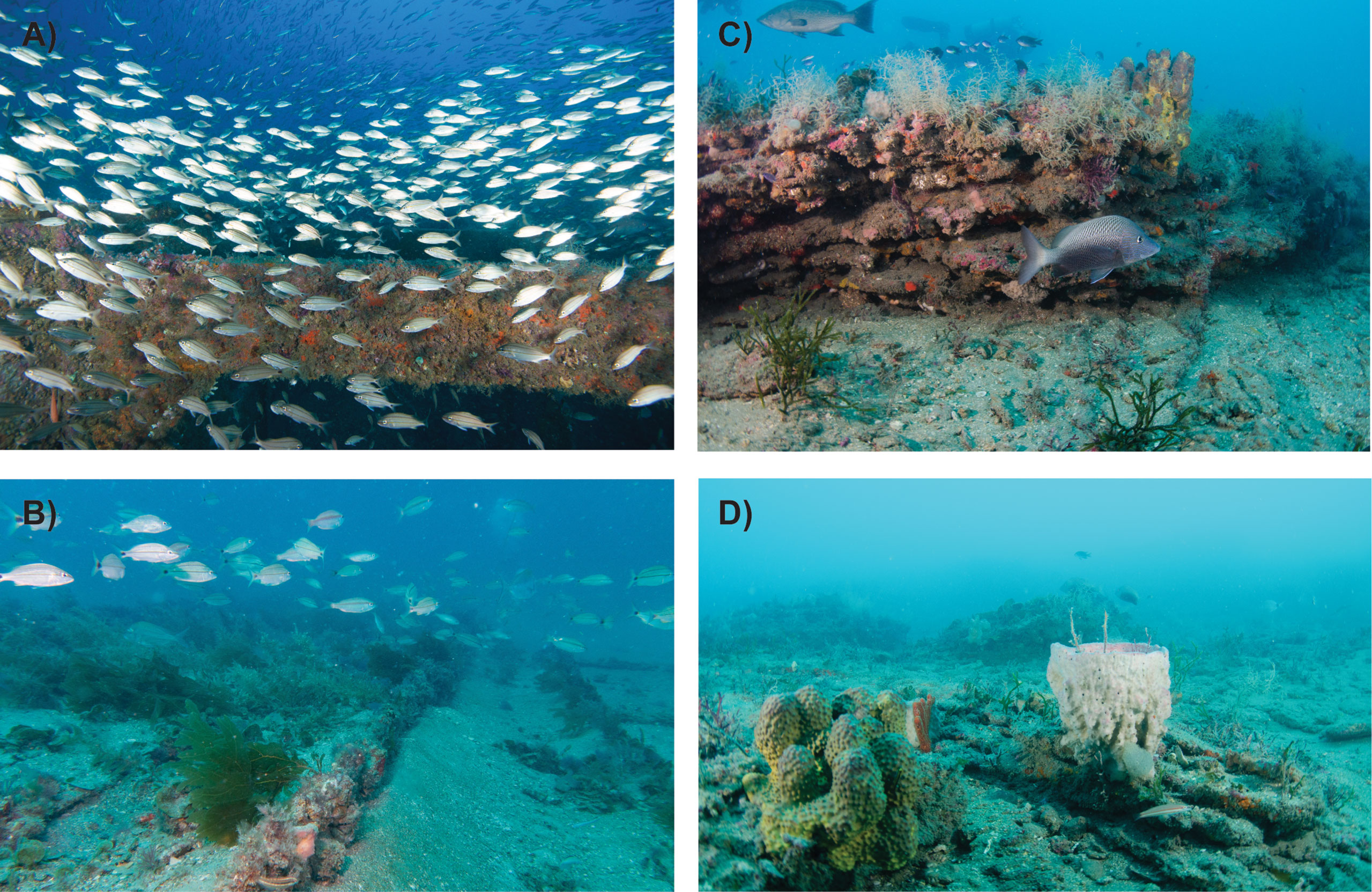
Figure 1 Underwater images of artificial reefs (A, B) and natural reefs (C, D) on the southeast US continental shelf. (A) Artificial reef created by a ship. (B) Artificial reef formed from a train boxcar. (C) High-relief rocky reef. (D) Low-relief rocky reef. Photos by John McCord/Coastal Studies Institute (A), Cory Ames/NCCOS (B), Dave Sybert (C, D).

Natural reefs in the region are patchy (Powles and Barans, 1980; Parker et al., 1983; Schobernd and Sedberry, 2009) and highly variable in size, structure, and composition, ranging from high-relief rocky ledges and outcrops to flat pavement sometimes covered by a veneer of sand (Barans and Henry, 1984; Parker Jr. and Mays, 1998) (Figures 1C, D). Because of their patchy and variable nature, natural reef extent has rarely been estimated in the SEUS and seafloor coverage estimates using limited data range from 3% to 30%. The most comprehensive study to estimate the extent of natural reefs in the SEUS used a stratified random sampling design and estimated that 30% of the seafloor between Cape Fear, North Carolina, and Cape Canaveral, Florida (27–101 m deep), was composed of natural reefs, and that natural reef coverage varied geographically with less coverage (14% of the seafloor) between Cape Hatteras and Cape Fear, North Carolina (Parker et al., 1983). Others have informally estimated that 10% of the SEUS continental shelf constitutes natural reef habitat (Hedgpeth, 1957; Struhsaker, 1969), and Parker et al. (1983) cite various personal communications that estimated 3–5% of various parts of the SEUS seafloor were covered by natural reefs. Regardless of their extent, it is well documented that these natural reefs provide substrate for various species of attached biota, such as sponges, soft corals, and algae, and together these natural reefs with attached biota provide important habitat for a diverse reef-associated fish community (Bacheler et al., 2019).

We develop and implement a reproducible and easily standardized approach for estimating the extent of artificial and natural reefs in the SEUS. Additionally, we compare the resulting reef extent estimates by reef type (artificial versus natural) and examine patterns in reef extent over the entire SEUS region, by state, and by depth. For artificial reefs, specifically, we also examine reef coverage by the material from which the artificial reef is constructed. While our case study was conducted for reefs in the SEUS, this approach is translatable to other large marine ecosystems to help better understand the relative coverage and spatial distribution of habitats, with implications for marine spatial planning and ecosystem-based fisheries management.

Materials and methods

Geographic scope

We compared artificial and natural reef extent in the SEUS (Figure 1), which we defined as bounded to the north by Cape Hatteras, NC (35.25° N latitude) and to the south by Port St. Lucie, FL (27.10° N latitude; Figure S1). Port St. Lucie was the southern boundary of our comparison because the transition from hard-bottom or rocky reefs to reef-building corals generally occurs south of this location. Depth was constrained to the continental shelf and upper slope between 10 m and 200 m for the comparison. Ten meters was selected as the shallowest extent for our analysis because current fishery sampling assessments for reef associated species and associated natural reef habitat begin at 10 m. Two hundred meters was selected as the deepest depth cutoff as this is the generally accepted limit of the upper continental slope off the SEUS (Wenner and Barans, 2001).

We developed multiple approaches, as described below, for quantifying the extent of artificial and natural reefs in the SEUS region, by state (North Carolina (NC), South Carolina (SC), Georgia (GA), Florida (FL)), and by depth bins (Figure S1). We defined state boundaries based on the Bureau of Ocean Energy Management (BOEM) administrative boundaries established for offshore energy planning and development (https://www.boem.gov/oil-gas-energy/mapping-and-data/map-gallery/administrative-boundaries, accessed 12/9/21). We binned depth at a fine resolution (10 m) for depths 10 m to 100 m and at a coarser resolution (100 m) for depths 100 m to 200 m, past the shelf break.

Artificial reefs

Data acquisition

Artificial reef data from four SEUS states – NC, SC, GA, FL – were obtained from the NC Division of Marine Fisheries, SC Department of Natural Resources, GA Department of Natural Resources – Coastal Resources Division, and FL Division of Marine Fisheries Management – Artificial Reef Program. Two data types were provided: 1) data on permitted artificial reef zones and 2) data on reef structures that occur in these zones.

Artificial reef plots

Data on permitted artificial reef zones or plots, which are areas in the coastal ocean officially designated through the permitting process as locations where artificial reefs can be deployed, included the reef plot coordinates (decimal degrees), depth (m), minimum permitted vertical clearance above the artificial reef (m), plot area (km²), deployment date, and special management zone (SMZ) designation, if applicable. We collated plot data from each state into one SEUS regional dataset such that all data were in standardized formats necessary for extent calculations. All data cleaning, collation, and analysis were conducted using ArcGIS Pro (ESRI, 2021) and R (R Development Core Team, 2021).

Artificial reef structures

Artificial reef structures deployed within permitted plots include items such as ships, concrete pipes, and concrete modules. Data for each structure included the permitted plot that the structure was deployed within, as well as the coordinates of the structure deployment. In some cases, we received depth information on the structures, but in most cases, we used depth collected at the level of the permitted plot and applied it to each structure within the plot. Data on the quantity of structure deployed, including the count (e.g., 100 units), tonnage, and for vessels, the vessel length (m), were provided for most structures, but unavailable for others. Each structure was also categorized more broadly (e.g., concrete pipes, steel vessel, train boxcars, bridge pieces, unknown) and sometimes accompanied by a more qualitative description (e.g., 330 ft barge, 75 Reef Balls, 925 tons of concrete pipe). We standardized and collated structure data from each state into one regional structures dataset.

There were 137 unique structure classifications across the four SEUS states. We categorized each of the 137 unique structure classifications into 25 broad categories to streamline the diverse structure types and nomenclature across states (Table S1). Each structure category reflected a combination of material (metal, concrete, rubber, wood, plastic, rock, fiberglass, unknown), structure (e.g., secondary use, modules, bridges, unspecified, vessels, tires, aircraft), and in some cases a sub-type further describing the structure attributes (e.g., long and skinny shaped, squat and block shaped, large vs. small, vessel size category). We also assigned each structure as low relief (< 2 m height) or high relief (> 2 m height) and as having a low, medium, or high rate of degradation.

Footprint calculation

Three data-driven approaches were developed to quantify the extent or footprint of artificial reefs within the SEUS artificial reef programs. Multiple approaches were necessary as each state had differing levels of information on artificial reefs. For example, NC conducted high-resolution habitat mapping of their artificial reefs and had precise estimates of artificial reef footprint, whereas others had not conducted habitat mapping but had quantity data for some structures.

Plot extent (all SEUS states)

We calculated the area of permitted artificial reef plots using the raster package (Hijmans, 2020) in R. The plot areas represent the total possible coverage of artificial reefs since no plots are fully covered by artificial reef structures.

Structure extent - measured (NC)

When artificial reef data included accurate measurements of the amount of area covered by structures in each plot, we used these measurements to calculate artificial reef extent. This approach, which we refer to as the “measured extent” method, was applicable when states had conducted habitat mapping surveys of artificial reefs using instruments, such as multibeam echosounders or side-scan sonar, that permitted delineation of artificial reef structures to calculate footprints. We applied the measured extent method to NC artificial reefs because NC artificial reefs had been mapped using side-scan sonar following an extensive multi-year mapping effort by the NC Artificial Reef Program, from which artificial reef structures were manually delineated for area calculations.

Structure extent - plot percentage (SC, GA, FL)

When measured structure footprints were unavailable, we estimated the extent of artificial reef structures as a percentage of the permitted plot area. This approach, which we refer to as the “plot percentage” method, used NC data to extrapolate to other states. We calculated the mean (0.57%), minimum (0.005%), and maximum (4.07%) percentage of artificial reef plots covered by artificial reef structures. We applied the mean, minimum, and maximum structure extents to permitted plots in SC, GA, and FL by multiplying the artificial reef plot sizes in each state by the NC mean, minimum, and maximum values to obtain an estimated mean, minimum, and maximum coverage value for each SEUS plot.

Structure extent - classified structures (SC, GA, FL)

The third approach for estimating structure extent, called the “classified structures” method, was based upon the footprint of particular structures, such as concrete pipes or large metal vessels. For each of the 25 broad structure categories (Table S1), we estimated footprints as follows. Structures from NC and some from FL were associated with measured footprint values. Some additional structures in FL had model-predicted footprints from a generalized linear model using a power-link function. This model was developed by the FL Artificial Reef Program and used the tonnage of material deployed as a parameter to predict the artificial reef footprint. These measured and modeled values provided footprints for discrete deployments of artificial reef structures. In cases where dimensions (e.g., 20 ft x 20 ft) but not footprints were provided, we used dimensions to calculate footprint. Some of the footprint values also had quantity data, either counts (e.g., a deployment of 500 concrete pipe), tons (a deployment of 100 tons of concrete pipe), or in some cases both count and tonnage values, associated with them. We used these footprint and quantity data to calculate unit footprint as m²/count or m²/ton and then to calculate the unit footprint minimum, mean, and maximum across deployments for each structure type. When quantity (count, tons) but not footprint data were available, we applied the minimum, mean, and maximum unit footprint values and multiplied them by the reported quantity. Footprints per count were preferred and used when available, otherwise we used footprints per ton. When neither quantity nor footprint values were provided for a structure deployment, we obtained footprint estimates from artificial reef managers or found the minimum, mean, and maximum footprints of all deployments (not per unit) of the same structure type across states and applied those values to estimate footprint. For structures with no measured values in the SEUS or manager-estimated footprint values, values were obtained from outside the SEUS from other artificial reef data. Calculating the mean, minimum, and maximum footprint values in a hierarchical fashion (e.g., first for structures with quantity, prioritizing count vs. ton, etc.) helped estimate uncertainty since there were likely variations in structures within each category (e.g., secondary-use concrete with long or skinny shapes included pipes, pilings, and culverts).

Natural reefs

The seafloor of the SEUS mostly consists of sand or mud, but patches of natural reef habitats occur throughout the region (Powles and Barans, 1980; Parker et al., 1983; Schobernd and Sedberry, 2009). Given the large discrepancies in previous estimates of natural reef extent in the SEUS that range from 3% to 30%, we provide updated estimates of the extent of natural reefs in the SEUS using three approaches: 1) polygon delineation, 2) regional synthesis, and 3) predictive model.

Polygon delineation

We delineated polygons corresponding to natural reefs using a spatial dataset of sonar mapping, survey data, and information from fishers in the SEUS (Text S2). Two coauthors (CMS, NMB) independently delineated estimated boundaries of natural reefs in ArcGIS Pro. In most cases, the size and shape of natural reef areas were obvious from the multiple data source layers (e.g., dozens of fishing points on top of a clear natural reef from the multibeam sonar map). In some cases, however, there were sparse points from fishers and no other correlating evidence of natural reefs in an area, so coauthors used their best judgment (independently) to determine if these points indicated a natural reef.

Because natural reefs are patchy and often occur as a matrix of rock and sand, drawing a polygon around this matrix of natural reef and sand would likely overestimate the amount of natural reef inside of the polygons. Low profile or pavement type reefs face exposure and burial by sediment movement influencing their detectability (Renaud et al., 1997). In addition, by drawing polygons around only obvious natural reefs, patches of natural reef habitat would likely be missed outside of the polygons. Thus, we estimated the extent of natural reefs in the SEUS region, by state, and by depth bin using three scenarios. The first scenario was designed as a low estimate of the extent of natural reef, assuming only 50% of the area inside and 0% outside of polygons was natural reef. The second scenario was designed as our best approximation of the extent of natural reefs, assuming 50% of the area inside and 1% outside of polygons was natural reef. Our third scenario was designed as a high estimate of natural reef, assuming 100% of the area inside and 2% of the area outside of polygons was natural reef. This approach resulted in six total estimates of natural reef extent in each stratum using the polygon delineation approach: estimates from two people and three scenarios. From these six estimates, we calculated mean and variance of the extent of natural hard-bottom for the overall SEUS, as well as by state and depth strata.

Regional synthesis - TNC synthesis

The second broad approach to estimate the extent of natural reefs in the SEUS used previously published thematic seafloor habitat classification maps from a regional synthesis conducted by The Nature Conservancy (TNC), called the South Atlantic Bight Marine Assessment (SABMA). SABMA is a synthesis and assessment of publicly available data and literature review on depth, seafloor complexity, geology, and sediments that classifies and defines seafloor habitats from tidal estuary to the outer continental shelf from the NC-VA state boundary to FL Keys (Conley et al., 2017). To quantify the distribution of natural reef habitats we restricted selection of habitat classes in the dataset to “hard-bottom slope” and “shelf upper slope” and only considered polygons that had confidence rankings from the review process of “probable”, “high confidence”, and “very high confidence” and omitted confidence rankings of “possible” and “potential”. The resulting polygons were converted and gridded into a raster layer with square cell dimensions of 90 m. The habitat classes were then reclassified to a binary value, where hard-bottom is 1 and no hard-bottom is 0.

Predictive habitat model - NCCOS model

The third natural reef estimation method was a hard-bottom likelihood map of the SEUS region from a predictive habitat model that was described in Pickens and Taylor (2020). We refer to this model as the NCCOS (NOAA National Centers for Coastal Ocean Science) model. The NCCOS model uses a spatially-explicit likelihood-based approach with derivatives of seafloor complexity as predictor variables and a Maximum Entropy model using bootstrapping to assess accuracy. Observations from fishery-independent surveys and compilations from sediment sampling databases were used to validate model predictions (Pickens and Tayor, 2020). The model output was a raster grid with cell resolution of 90 m by 90 m. We applied a threshold of likelihood values >0.63, which represented an accuracy of greater than 90% at predicting the occurrence of hard-bottom within the grid cell and a <5% false positivity rate. This threshold was used to reclassify into a binary raster with cell resolution 90 m by 90 m.

We also assessed another predictive model for hard-bottom distribution in the SEUS from Dunn and Halpin (2009) but did not include this model in our estimation approaches because it exhibited biases (Text S1).

Results

Multiple data-driven approaches quantifying the amount of seafloor in the SEUS covered by artificial and natural reefs revealed that artificial reefs account for several orders of magnitude less habitat than natural reefs (Figures 2, 3; Table 1). Of the entire SEUS region (103,220 km²), permitted artificial reef zones comprise 705 km² (0.68%) of the seafloor (Figure S2). Permitted extent of artificial reef zones is an overestimate of the amount of seafloor covered by artificial reefs because the zones are not completely covered with artificial reef structures (Table 1). Estimates of structure extent based on percent coverage of permitted zones (plot percentage method) indicated that 4.02 km² (<0.01%) of the SEUS seafloor is covered by artificial reefs (Figure 3A; Tables 1; S2). When we estimated artificial reef coverage based on different structure classifications (e.g., concrete pipes, metal vessels), our calculations suggested that a smaller area, 1.98 km² (<0.01%), of the SEUS is covered with artificial reef structures (Figure 3A; Tables 1, S2). Averaging results from the plot percentage and classified structures approaches resulted in an estimate of 3.00 km² (<0.01%) of the SEUS seafloor covered by artificial reefs.

FIGURE 2

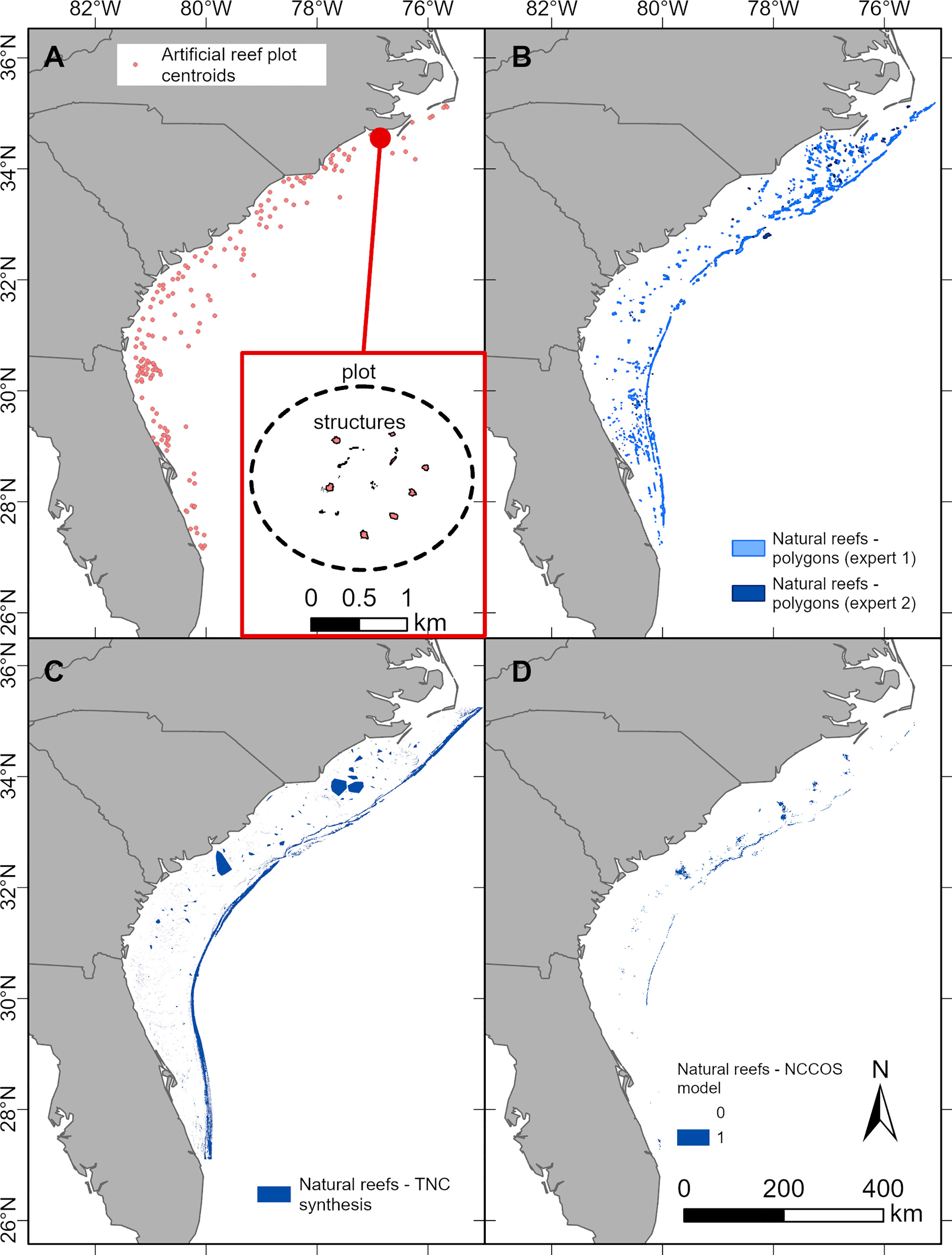
Figure 2 Locations of artificial reefs (A) and natural reefs (B–D) along the southeastern US continental shelf. (A) Artificial reef locations correspond to centroids of permitted artificial reef plots, and the size of the artificial reef dots corresponding to each plot is not to scale. The inset in panel A depicts one NC artificial reef permitted plot (dashed line) and the artificial reef structures (red polygons) within. (B) Natural reefs delineated by expert-drawn polygons. (C) Natural reefs predicted by the TNC synthesis. (D) Natural reefs predicted by the NCCOS model (likelihood >0.63).

FIGURE 3

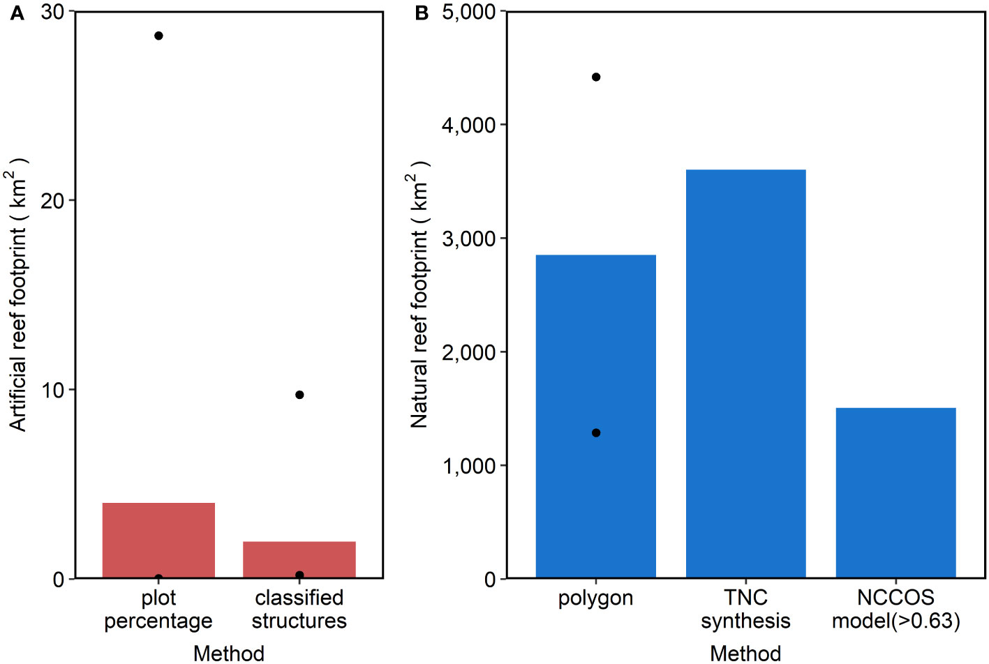
Figure 3 Extent of artificial reefs (A, red) and natural reefs (B, blue) for the entire SEUS region. Measured approach for artificial reef footprint not shown because only applied to NC. Black circles represent the maximum and minimum extent values for applicable methods. Note different y-axis scales.

TABLE 1

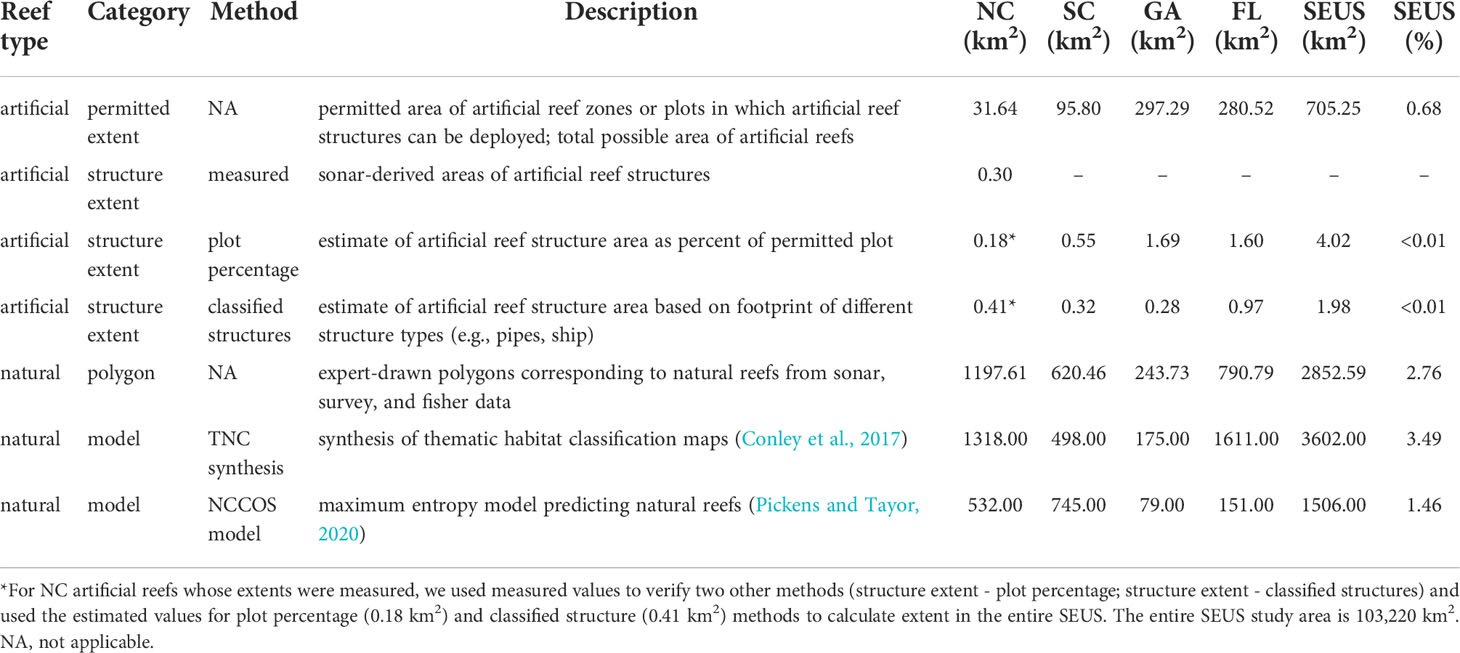
Table 1 Approaches for and corresponding estimates of artificial and natural reef extents.

Estimates of natural reef extent, in contrast, far exceeded those of artificial reef extent in the SEUS. The three natural reef extent methods predicted an average of 2,654 km² (2.57%) of the SEUS covered by natural reefs (Figure 3B; Tables 1, S3). The TNC synthesis model suggested the highest coverage (3,602.0 km², 3.49%), followed by expert drawn polygons (2,852.59 km², 2.76%), and the NCCOS maximum entropy model (1,506.00 km², 1.46%; Figure 3B; Tables 1, S3).

The pattern of artificial reefs covering orders of magnitude less seafloor than natural reefs held across each of the four SEUS states (Figure 4; Table 1). While measured footprints based on seafloor mapping provided the best estimate of artificial reef extent in NC, we also calculated extent based on plot percentage and classified structures as a means of validating these two methods before applying to SC, GA, and FL (Figure 4A; Tables 1, S2). Coverage estimates based on plot percentages consistently exceeded estimates based on classified structures in SC, GA, and FL. For natural reefs, the TNC synthesis predicted the highest coverage for FL, whereas the NCCOS model predicted the highest coverage in SC and the polygon method predicted the highest in NC (Figure 4B; Tables 1, S3). Each artificial reef estimation method was several orders of magnitude less than its respective natural reef estimation.

FIGURE 4

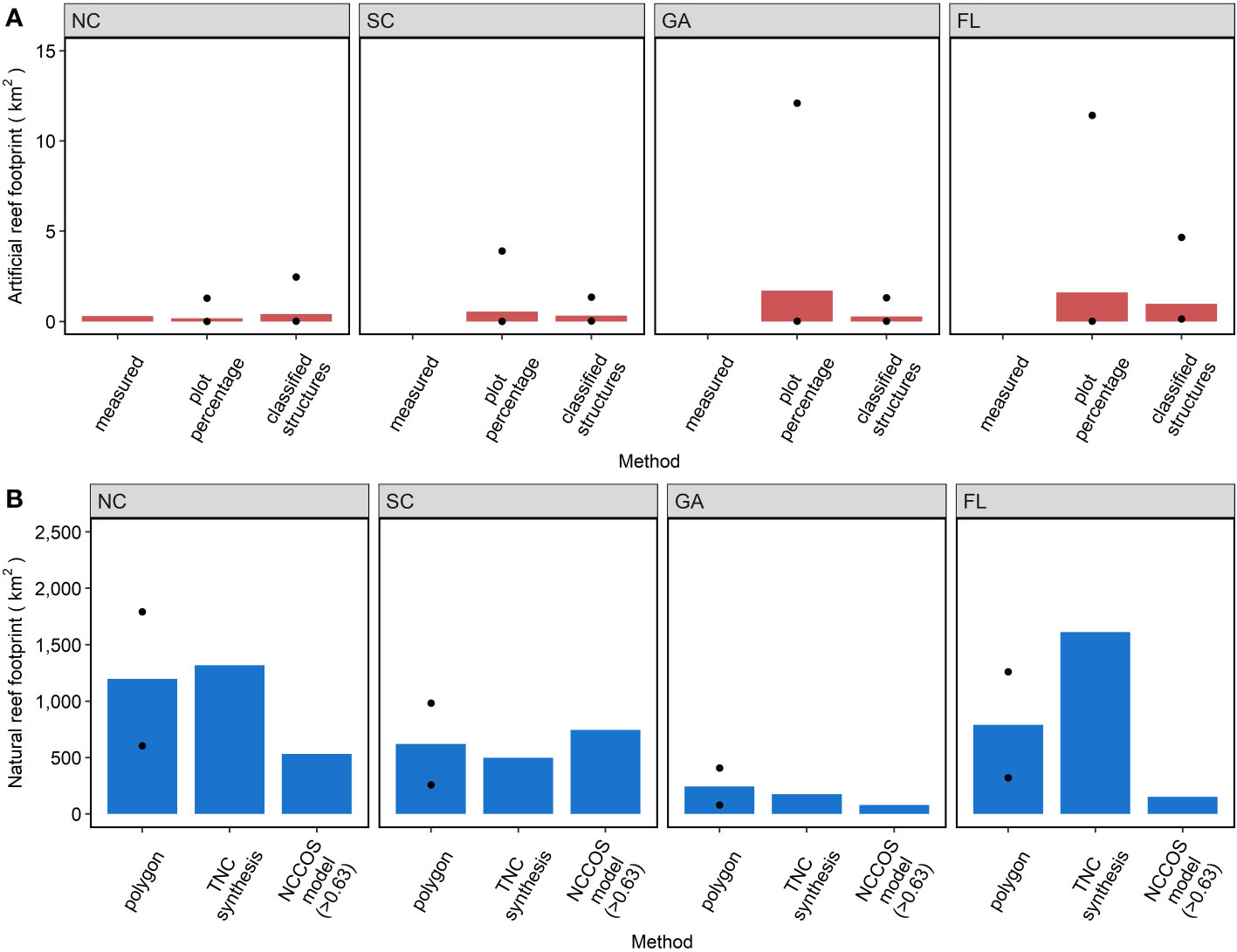
Figure 4 Footprint (km²) of artificial reefs (A, red) and natural reefs (B, blue) by state (columns). Measured approach for artificial reef footprint was only available in NC. Black circles represent the maximum and minimum extent values for applicable methods. Note different y-axis scales between panels (A, B).

Natural reef coverage surpassed that of artificial reefs across SEUS depths ranging from 10 m to 200 m (Figure 5). The deepest artificial reef documented in our study rests in 90 - 100 m, and most occur shallower than 60 m (Figure 5A; Table S2). In contrast, natural reefs were more widely distributed across the continental shelf up to the 200 m cut-off of the study, representing the upper continental slope (Figure 5B; Table S3). The three estimates of natural reef coverage exhibited different patterns. In the NCCOS model, natural reefs were concentrated in shallower depths, whereas in the TNC synthesis the opposite trend was observed. In the expert-based polygon approach, natural reefs were more universally distributed across the depth range.

FIGURE 5

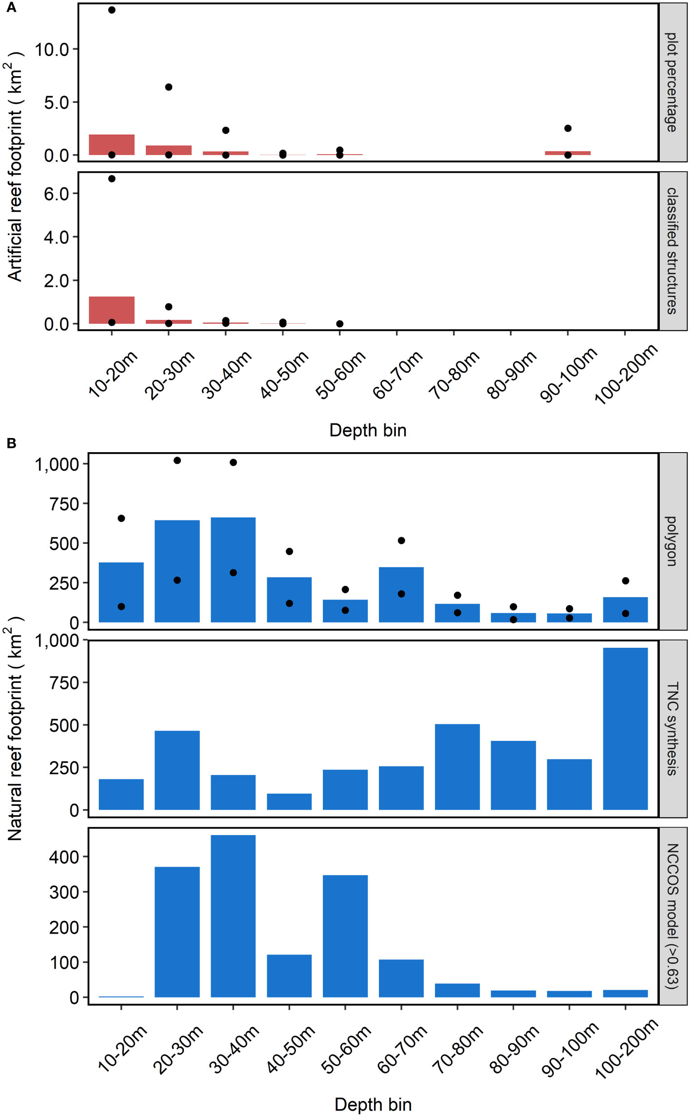
Figure 5 Extent of artificial reefs (A) and natural reefs (B) by depth bin. Measured approach for artificial reef footprint not shown because only applied to NC. Twelve artificial reefs did not have assigned values, so these artificial reefs permitted plots and structures are not represented in this figure. Black circles represent the maximum and minimum extent values for applicable methods. Note different y-axis scales between panels (A, B).

Analysis of the types of artificial reef structures in the SEUS revealed a diversity of structure materials (e.g., concrete, metal) and types (e.g., bridges, modules) (Table S1). Throughout the SEUS, secondary-use concrete structures with a long-skinny shape, such as concrete pipes, were deployed most frequently (449 deployments), followed by medium-sized metal vessels (249 deployments), trains and containers (220 deployments), small concrete modules (199 deployments), and long-lived metal vehicles (146 deployments; Figure S3; Table S1). The structures with the largest regional footprint were secondary-use concrete structures with a long-skinny shape (0.78 km²), followed by concrete bridges (0.34 km²), unspecified concrete (0.27 km²), small concrete modules (0.12 km²), and secondary-use concrete structures with a squat-block shape (0.10 km²; Figure S3; Table S1).

Discussion

Our evaluation of artificial versus natural reef extent indicates that the amount of seafloor covered by artificial reefs in the SEUS is several orders of magnitude less than that of natural reefs. Across the SEUS region (103,220 km²), artificial reef extent (3 km², averaged across methods) was 885 times less than natural reef extent (2,654 km²). This pattern of more extensive natural reef extent was consistent across state and depth groupings. To our knowledge, ours is the first estimate of artificial reef extent in the SEUS. Prior estimates of natural reefs in the region vary dramatically from 3% to 30% (Hedgpeth, 1957; Struhsaker, 1969; Parker et al., 1983). Our estimates based on seafloor maps and published geological and predictive seafloor habitat models suggest that natural reef coverage is less than previous estimates at 2.57% (average of our three approaches) of the SEUS seafloor.

Our SEUS regional estimates suggesting that artificial reefs are a “drop in the bucket” compared to natural reefs are similar to estimates of reef type extent in other geographic regions. A recent synthesis of seafloor mapping data on the eastern Gulf of Mexico (GOM) continental shelf extrapolated that 2.6% of the seafloor is covered in natural reefs (Keenan et al., 2022), which similarly helped refine previous natural reef coverage estimates that ranged from 13% (Jaap, 2015) based on Rohmann et al. (2005) to 38% (Parker et al., 1983). While Keenan et al. did not extrapolate artificial reef coverage across the eastern GOM, they did delineate both artificial and natural reefs from their seafloor mapping dataset that covered a subset of the eastern GOM. These non-extrapolated seafloor mapping data interpretations demonstrated that artificial reefs are several orders of magnitude less than natural reefs (2.2 km² artificial reefs versus 226.2 km² natural reefs delineated) in the eastern GOM. Likewise, in a small portion of the Florida Reef Tract (Martin County, FL), habitat mapping data identified that 0.66% of the region was artificial structure whereas 4.13% was colonized pavement and coral reefs (Walker and Gilliam, 2013).

Patterns in artificial versus natural reef extent observed over the SEUS region translated to finer groupings of states and depth zones. While artificial and natural reef extent estimates varied based on the estimation method, all states exhibited substantially less seafloor covered by artificial reefs than by natural reefs. In NC, for example, the measured footprint of artificial reefs was four orders of magnitude less than each natural reef extent estimate. The same pattern of heightened natural reef coverage applied across depth bins. Artificial reefs had greater proportional coverage in shallower depths, likely reflecting artificial reef deployment goals, which often include providing fishing and diving sites that are easily accessible by stakeholders and thus close to shore in shallower depths (Becker et al., 2018; Paxton et al., 2022). Natural reefs, however, are more widespread across depth gradients and are susceptible to burial and exposure with sediment movement, reflecting the underlying geology of the SEUS region (Parker et al., 1983; Riggs et al., 1996; Renaud et al., 1997; Riggs et al., 1998).

Despite their relatively small footprint (<0.01% of seafloor) in the SEUS, these artificial reefs play key ecological roles within the seascape. Within the SEUS region, for example, artificial reefs have been shown to host high abundances of tropical and subtropical reef fish at their poleward climate range edges (Paxton et al., 2019b) and high densities of large predators (Paxton et al., 2020), potentially provide stepping stones or connectivity corridors for large predator movement (Paxton et al., 2019a), and form hotspots for economically valuable fish species (Paxton et al., 2021). The fish communities on artificial reefs differ from those of nearby natural reefs (Paxton et al., 2017; Rosemond et al., 2018; Lemoine et al., 2019) and this translates to differences in species-specific feeding ecology (Lindquist et al., 1994; Pike and Lindquist, 1994). Additionally, findings outside of the SEUS in shallow urbanized estuaries indicate that artificial reefs have the potential to exacerbate the spread of invasive species (Dafforn et al., 2012; Airoldi et al., 2015) and pose other risks, such as aggregating fish away from natural reefs (Bohnsack, 1989; Layman et al., 2016). Given the ecological functions of artificial reefs, they have the potential to drive change by affecting ecosystem patterns and processes (Bulleri and Chapman, 2010; Dafforn et al., 2015; Bishop et al., 2017; Heery et al., 2017) and by hosting fish communities that differ long-term from those on nearby natural reefs (Becker et al., 2022). Potential ecological ramifications, including both benefits and risks, of artificial reef placement in the seascape cement a future research need to incorporate footprint estimations into ecological projections of artificial reef effects.

There are numerous economically and ecologically important fish species that associate with natural and artificial reefs in the SEUS (Bacheler et al., 2019), and knowing the extent and spatial arrangement of natural reefs can improve their management in several ways. For instance, estimating the total abundance of reef-associated fish species precisely and accurately would be beneficial for reef fish management, as evidenced by the millions of dollars of recent federal funding to estimate red snapper (Lutjanus campechanus; (Stunz et al., 2021); https://www.scseagrant.org/sc-sea-grant-award-red-snapper-count/) and greater amberjack (Seriola dumerili; https://masgc.org/news/article/team-selected-to-estimate-abundance-of-greater-amberjack-in-south-atlantic) absolute abundance in the SEUS and the GOM. With detailed knowledge of the extent of natural and artificial reefs, fish densities could be estimated more accurately and also incorporated into long-term studies, similar to Becker et al. (2022). Another benefit of knowing the spatial arrangement of natural reef habitats in the SEUS is in guiding marine spatial planning, including marine protected area placement and placement of future artificial reefs in the region, since artificial reefs are often installed to supplement existing natural reefs.

Fish are known to concentrate at artificial reefs, but there is disagreement about whether they might add or subtract fish biomass from natural reefs (Bohnsack, 1989; Powers et al., 2003). Artificial reefs may attract fish away from natural reefs (“attraction hypothesis”), which would increase abundance at artificial reefs at the expense of natural reefs and facilitate exploitation by fishers (Grossman et al., 1997). In contrast, artificial reefs may support additional fish production (“production hypothesis”), which would not reduce biomass in natural reefs (Folpp et al., 2020). Regardless of whether aggregation, production, or a blend of both occurs on artificial reefs, artificial reefs are often deployed to enhance fish habitat, forming locations for recreational fishing. Fishing pressure at artificial reefs has not been well-quantified in the SEUS; however, findings from the FL GOM coast suggest high fishing pressure occurs on artificial reefs. For example, recreational reef fish angler surveys revealed that 46% of angler trips seeking reef fish targeted artificial reefs (Cross et al., 2018). Additionally, recreational anglers anecdotally perceive that artificial reefs experience high fishing pressure based on observations of recreational vessel congestion. Given our finding that artificial reefs cover a relatively small amount of SEUS seafloor compared to natural reefs, if heightened fishing pressure on artificial reefs manifests across the SEUS, then small, island-like artificial reefs could be receiving a disproportionate amount of recreational fishing pressure. The designation of artificial reefs in federal waters as Special Management Zones (SMZs), which already existed off SC and have recently been completed and codified in NC through the South Atlantic Fishery Management Council, could prevent inequitable fishing by restricting high-efficiency gears. Directing fishing pressure to artificial reefs instead of natural reefs has ecological implications, potentially establishing natural reefs as refugia from fishing pressure while depleting fish populations at artificial reefs (Solonsky, 1985; Addis et al., 2016). With these scenarios in mind, region-wide reef fish sampling programs could consider sampling artificial reefs concurrently with sampled natural reefs to quantify reef-associated fish communities and potential effects from differential fishing pressure on these two types of structured habitat.

Estimating the extent of artificial reefs was challenging because it involved synthesizing disparate data across a broad geographic region. The methods we developed effectively standardized artificial reef data across states, enabling region-wide analysis, and ultimately comparison with natural reef data. When we validated the plot percentage estimate by performing the estimation in NC and comparing it to the measured NC footprint, we found that the plot percentage approach underestimated the artificial reef footprint. However, when extrapolated to SC, GA, and FL, this method likely overestimated coverage, as NC permitted zones were typically filled with a higher portion of structures than those in the other states. This discrepancy likely reflects different artificial reef development strategies between states. For example, NC rarely established new artificial reef plots, preferring to continue to develop within existing permitted zones, which could explain the inflated artificial reef estimates for reefs in other states. And, in some states, sandy habitat within permitted plots is intentionally left devoid of artificial reef structures to provide foraging grounds for select fish species. When we validated the classified structure method in NC, it overpredicted NC coverage compared to the measured footprint. Despite the overprediction in NC, the structure classification estimate accounted for the diversity of artificial reef structure types deployed on the SEUS seafloor and in general estimated a smaller footprint than the plot percentage method. The true coverage of artificial reefs likely falls between the plot percentage and classified structure estimates. In the future, additional habitat mapping efforts following artificial reef deployment would allow delineation of the footprint of deployed artificial reef structures and could help streamline this approach and refine estimates.

The three approaches to estimating natural reef extent had respective strengths and weaknesses. First, the polygon approach resulted in natural reef extent estimates that were between those predicted by the other two methods, the TNC synthesis and NCCOS model, in all states except GA. Second, the TNC synthesis predicted the highest NR extent compared to the other methods in NC and FL and predicted high natural reef coverage between 100-200 m depths. Third, the NCCOS maximum entropy model predicted the lowest NR extent in all states except SC. This model seemingly underpredicted natural reef extent in the shallowest and deepest depth groupings. This could be explained by the considerable change in relative seafloor complexity from the relatively flat, shallow shelf waters, through the steep slope of the shelf edge to the lower slope of the continental shelf. The true coverage of natural reefs likely falls within the three natural reef estimation approaches. More extensive and concentrated habitat mapping and ground-truthing approaches along the SEUS continental shelf will help improve natural reef extent estimates.

This study fills gaps in and establishes baseline understanding of artificial and natural reef coverage on the SEUS seafloor by generating the first estimate of artificial reef footprint in the SEUS and simultaneously refining previous regional natural reef extent estimates. It also identified gaps, such as the need for more expansive, but also finer scale, seafloor mapping and characterization efforts for both artificial and natural reefs along with a more standardized approach to recording and managing quantitative information on artificial reef deployments. With projected increases in artificial structures globally, including slated offshore wind energy development, and potential reef-related impacts from climate change, the reproducible approach that we developed for quantifying reef footprint is applicable to other geographic regions and ultimately provides support for regional marine spatial planning needs and accompanying ecosystem-based management.

Data availability statement

The original contributions presented in the study are included in the article/Supplementary Material. Further inquiries can be directed to the corresponding authors.

Author contributions

GK, AP, NB, and JT conceived of this research. KM and JR provided Florida artificial reef data. ZH and JB provided North Carolina artificial reef data. RM and CB provided South Carolina and Georgia artificial reef data, respectively. DS and AP processed artificial reef data. NB and CS delineated natural reef polygons and performed associated calculations. JT acquired natural reef habitat synthesis and predictive models and calculated the extent of natural reefs from these. DS and AP conducted comparative analyses for artificial and natural reef extents and created figures and tables. DS, AP, and NB drafted the manuscript. All authors contributed to the article and approved the submitted version.

Funding

CSS-Inc was not involved in the study design, collection, analysis, interpretation of data, the writing of this article or the decision to submit it for publication.

Acknowledgments

We thank the NOAA National Centers for Coastal Ocean Science for supporting this synthesis. DS was supported by Duke University Rachel Carson Scholars Program. AP was partially supported by CSS-Inc. under NOAA/NCCOS Contract #EA133C17BA0062. We thank M. Burton for thoughtful reviews of the manuscript. The views and conclusions contained in this document are those of the authors and should not be interpreted as representing the opinions or policies of the US Government, nor does mention of trade names or commercial products constitute endorsement or recommendation for use.

Conflict of interest

AP received partial support from CSS-Inc.

The remaining authors declare that the research was conducted in the absence of any commercial or financial relationships that could be construed as a potential conflict of interest.

Publisher’s note

All claims expressed in this article are solely those of the authors and do not necessarily represent those of their affiliated organizations, or those of the publisher, the editors and the reviewers. Any product that may be evaluated in this article, or claim that may be made by its manufacturer, is not guaranteed or endorsed by the publisher.

Supplementary material

The Supplementary Material for this article can be found online at: https://www.frontiersin.org/articles/10.3389/fmars.2022.980384/full#supplementary-material

References

Addis D. T., Patterson W. F., Dance M. A. (2016). The potential for unreported artificial reefs to serve as refuges from fishing mortality for reef fishes. North Am. J. Fisheries Manage. 36, 131–139. doi: 10.1080/02755947.2015.1084406

CrossRef Full Text | Google Scholar

Airoldi L., Turon X., Perkol-Finkel S., Rius M. (2015). Corridors for aliens but not for natives: Èffects of marine urban sprawl at a regional scale. Diversity Distributions 21, 755–768. doi: 10.1111/ddi.12301

CrossRef Full Text | Google Scholar

Bacheler N. M., Schobernd Z. H., Gregalis K. C., Schobernd C. M., Teer B. Z., Gillum Z., et al. (2019). Patterns in fish biodiversity associated with temperate reefs on the southeastern US continental shelf. Mar. Biodiversity 49, 2411–2428. doi: 10.1007/s12526-019-00981-9

CrossRef Full Text | Google Scholar

Bacheler N. M., Shertzer K. W. (2020). Catchability of reef fish species in traps is strongly affected by water temperature and substrate. Mar. Ecol. Prog. Ser. 642, 179–190. doi: 10.3354/meps13337

CrossRef Full Text | Google Scholar

Barans C. A., Henry V. J. (1984). A description of the shelf edge groundfish habitat along the southeastern united states. Northeast Gulf Sci. 7, 77–96. doi: 10.18785/negs.0701.05

CrossRef Full Text | Google Scholar

Becker A., Taylor M. D., Folpp H., Lowry M. B. (2018). Managing the development of artificial reef systems: The need for quantitative goals. Fish Fisheries 19, 740–752. doi: 10.1111/faf.12288

CrossRef Full Text | Google Scholar

Becker A., Taylor M., Folpp H., Lowry M. (2022). Revisiting an artificial reef after 10 years: What has changed and what remains the same? Fisheries Res. 249. doi: 10.1016/j.fishres.2022.106261

CrossRef Full Text | Google Scholar

Bishop M. J., Mayer-Pinto M., Airoldi L., Firth L. B., Morris R. L., Loke L. H. L., et al. (2017). Effects of ocean sprawl on ecological connectivity: Impacts and solutions. J. Exp. Mar. Biol. Ecol. 492, 7–30. doi: 10.1016/j.jembe.2017.01.021

CrossRef Full Text | Google Scholar

Bohnsack J. A. (1989). Are high densities of fishes at artificial reefs the result of habitat limitation or behavioral preference? Bull. Mar. Sci. 44, 631–645.

Google Scholar

Bugnot A. B., Mayer-Pinto M., Airoldi L., Heery E. C., Johnston E. L., Critchley L. P., et al. (2021). Current and projected global extent of marine built structures. Nat. Sustainability 4, 33–41. doi: 10.1038/s41893-020-00595-1

CrossRef Full Text | Google Scholar

Bulleri F., Airoldi L. (2005). Artificial marine structures facilitate the spread of a non-indigenous green alga, Codium fragile ssp. tomentosoides. North Adriatic Sea. J. Appl. Ecol. 42, 1063–1072. doi: 10.1111/j.1365-2664.2005.01096.x

CrossRef Full Text | Google Scholar

Bulleri F, Chapman M. G. (2010). The introduction of coastal infrastructure as a driver of change in marine environments. J. Appl. Ecol. 47, 26–35. doi: 10.1111/j.1365-2664.2009.01751.x

CrossRef Full Text | Google Scholar

Cannizzo Z. J., Griffen B. D. (2019). An artificial habitat facilitates a climate-mediated range expansion into a suboptimal novel ecosystem. PloS One 14, e0211638. doi: 10.1371/journal.pone.0211638

PubMed Abstract | CrossRef Full Text | Google Scholar

Champion C., Suthers I. M., Smith J. A. (2015). Zooplanktivory is a key process for fish production on a coastal artificial reef. Mar. Ecol. Prog. Ser. 541, 1–14. doi: 10.3354/meps11529

CrossRef Full Text | Google Scholar

Christiansen H. M., Switzer T. S., Brodie R. B., Solomon J. J., Paperno R. (2020). Indices of abundance for red snapper (Lutjanus campechanus) from the FWC fish and wildlife research institute (FWRI) repetitive timed drop survey in the U.S. south Atlantic (North Charleston, SC:SEDAR).

Google Scholar

Claisse J. T., Pondella D. J., Love M., Zahn L. A., Williams C. M., Williams J. P., et al. (2014). Oil platforms off California are among the most productive marine fish habitats globally. Proc. Natl. Acad. Sci. 111, 15462–15467. doi: 10.1073/pnas.1411477111

CrossRef Full Text | Google Scholar

Conley M. F., Anderson M. G., Steinberg N., Barnett A. (2017). The South Atlantic bight marine assessment: Species, habitats and ecosystems. Nat. Conservancy Eastern Conserv. Sci, 496 pp.

Google Scholar

Cross T. A., Sauls B., Germeroth R., Mille K. (2018). Methods to quantify recreational angling effort on artificial reefs off florida's gulf of Mexico coast. Am. Fisheries Soc. Symposium 86, 265–277.

Google Scholar

Dafforn K. A., Glasby T. M., Airoldi L., Rivero N. K., Mayer-Pinto M., Johnston E. L. (2015). Marine urbanization: An ecological framework for designing multifunctional artificial structures. Front. Ecol. Environ. 13, 82–90. doi: 10.1890/140050

CrossRef Full Text | Google Scholar

Dafforn K. A., Glasby T. M., Johnston E. L. (2012). Comparing the invasibility of experimental "reefs" with field observations of natural reefs and artificial structures. PloS One 7, e38124. doi: 10.1371/journal.pone.0038124

PubMed Abstract | CrossRef Full Text | Google Scholar

Development Core Team R. (2021). R: A language and environment for statistical computing (Vienna, Austria: R Foundation for Statistical Computing).

Google Scholar

Dugan J. E., Airoldi L., Chapman M. G., Walker S. J., Schlacher T. (2011). Estuarine and coastal structures: Environmental effects, a focus on shore and nearshore structuresWolanski E., McLusky D. S.. Treatise Estuar. Coast. Sci. 8, pp 17–41. Waltham:Academic Press. doi: 10.1016/B978-0-12-374711-2.00802.0

CrossRef Full Text | Google Scholar

Dunn D. C., Halpin P. N. (2009). Rugosity-based regional modeling of hard-bottom habitat. Mar. Ecol. Prog. Ser. 377, 1–11. doi: 10.3354/meps07839

CrossRef Full Text | Google Scholar

ESRI (2021). ArcGIS pro. redlands, California, USA. environmental systems research institute (Redlands, California, USA: Environmental Systems Research Institute).

Google Scholar

Firth L. B., Knights A. M., Bridger D., Evans A. J., Mieszkowska N., Moore P., et al. (2016). Ocean sprawl: Challenges and opportunities for biodiversity management in a changing world. Oceanography Mar. Biol.: Annu. Rev. 54, 189–262. doi: 10.1201/9781315368597-5

CrossRef Full Text | Google Scholar

Folpp H. R., Schilling H. T., Clark G. F., Lowry M. B., Maslen B., Gregson M., et al. (2020). Artificial reefs increase fish abundance in habitat-limited estuaries. J. Appl. Ecol. 57, 1752–1761. doi: 10.1111/1365-2664.13666

CrossRef Full Text | Google Scholar

Gates A. R., Horton T., Serpell-Stevens A., Chandler C., Grange L. J., Robert K., et al. (2019). Ecological role of an offshore industry artificial structure. Front. Mar. Sci. 6. doi: 10.3389/fmars.2019.00675

CrossRef Full Text | Google Scholar

Grossman G. D., Jones G. P., Seaman W. J. Jr. (1997). Do artificial reefs increase regional fish production? A review of existing data. Fisheries 22, 17–23. doi: 10.1577/1548-8446(1997)022<0017:DARIRF>2.0.CO;2

CrossRef Full Text | Google Scholar

Harter S. L., Ribera M. M., Shepard A. N., Reed J. K. (2008). Assessment of fish populations and habitat on oculina bank, a deep-sea coral marine protected area off eastern Florida. Fishery Bull. 107, 195–206.

Google Scholar

Hedgpeth J. W. (1957). Treatise on marine ecology and paleoecology. Geological Soc. America Memoir 1, 1296.

Google Scholar

Heery E. C., Bishop M. J., Critchley L. P., Bugnot A. B., Airoldi L., Mayer-Pinto M., et al. (2017). Identifying the consequences of ocean sprawl for sedimentary habitats. J. Exp. Mar. Biol. Ecol. 492, 31–48. doi: 10.1016/j.jembe.2017.01.020

CrossRef Full Text | Google Scholar

Hijmans R. J. (2020). Raster: Geographic data analysis and modeling. https://CRAN.R-project.org/package=raster

Google Scholar

Jaap W. C. (2015). Stony coral (Milleporidae and scleractinia) communities in the eastern gulf of Mexico: A synopsis with insights from the hourglass collections. Bull. Mar. Sci. 91, 207–253. doi: 10.5343/bms.2014.1049

CrossRef Full Text | Google Scholar

Keenan S. F., Switzer T. S., Knapp A., Weather E. J., Davis J. (2022). Spatial dynamics of the quantity and diversity of natural and artificial hard bottom habitats in the eastern gulf of Mexico. Continental Shelf Res. 233. doi: 10.1016/j.csr.2021.104633

CrossRef Full Text | Google Scholar

Layman C. A., Allgeier J. E., Montaña C. G. (2016). Mechanistic evidence of enhanced production on artificial reefs: A case study in a Bahamian seagrass ecosystem. Ecol. Eng. 95, 574–579. doi: 10.1016/j.ecoleng.2016.06.109

CrossRef Full Text | Google Scholar

Lee M. O., Otake S., Kim J. K. (2018). Transition of artificial reefs (ARs) research and its prospects. Ocean Coast. Manage. 154, 55–65. doi: 10.1016/j.ocecoaman.2018.01.010

CrossRef Full Text | Google Scholar

Lemoine H. R., Paxton A. B., Anisfeld S. C., Rosemond R. C., Peterson C. H. (2019). Selecting the optimal artificial reefs to achieve fish habitat enhancement goals. Biol. Conserv. 238. doi: 10.1016/j.biocon.2019.108200

PubMed Abstract | CrossRef Full Text | Google Scholar

Lindquist D. G., Cahoon L. B., Clavijo I. E., Posey M. H., Bolden S. K., Pike L. A., et al. (1994). Reef fish stomach contents and prey abundance on reef and sand substrata associated with adjacent artificial and natural reefs in onslow bay, north Carolina. Bull. Mar. Sci. 55, 308–318.

Google Scholar

Miller R. G., Hutchison Z. L., Macleod A. K., Burrows M. T., Cook E. J., Last K. S., et al. (2013). Marine renewable energy development: Assessing the benthic footprint at multiple scales. Front. Ecol. Environ. 11, 433–440. doi: 10.1890/120089

CrossRef Full Text | Google Scholar

Mitchell W. A., Kellison G. T., Bacheler N. M., Potts J. C., Schobernd C. M., Hale L. F. (2014). Depth-related distribution of postjuvenile red snapper in southeastern U.S. Atlantic ocean waters: Ontogenic patterns and implications for management. Mar. Coast. Fisheries 6, 142–155. doi: 10.1080/19425120.2014.920743

CrossRef Full Text | Google Scholar

Parker R., Colby D., Willis T. (1983). Estimated amount of reef habitat on a portion of the U.S. South Atlantic Gulf Mexico Continental Shelf. Bull. Mar. Sci. 33, 935–940.

Google Scholar

Parker R. O. Jr., Mays R. W. (1998). Southeastern u. s. deepwater reef fish assemblages, habitat characteristics, catches, and life history summaries. NOAA Technical Report, NMFS 138, 41

Google Scholar

Paxton A. B., Blair E., Blawas C., Fatzinger M. H., Marens M., Holmberg J., et al. (2019a). Citizen science reveals female sand tiger sharks (Carcharias taurus) exhibit signs of site fidelity on shipwrecks. Ecology 100, e02687. doi: 10.1002/ecy.2687

PubMed Abstract | CrossRef Full Text | Google Scholar

Paxton A. B., Harter S. L., Ross S. W., Schobernd C. M., Runde B. J., Rudershausen P. J., et al. (2021). Four decades of reef observations illuminate deep-water grouper hotspots. Fish Fisheries 22, 749–761. doi: 10.1111/faf.12548

CrossRef Full Text | Google Scholar

Paxton A. B., Newton E. A., Adler A. M., Van Hoeck R. V., Iversen E. S. Jr., Taylor J. C., et al. (2020). Artificial habitats host elevated densities of large reef-associated predators. PloS One 15, e0237374. doi: 10.1371/journal.pone.0237374

PubMed Abstract | CrossRef Full Text | Google Scholar

Paxton A. B., Peterson C. H., Taylor J. C., Adler A. M., Pickering E. A., Silliman B. R. (2019b). Artificial reefs facilitate tropical fish at their range edge. Commun. Biol. 2, 168. doi: 10.1038/s42003-019-0398-2

PubMed Abstract | CrossRef Full Text | Google Scholar

Paxton A. B., Pickering E. A., Adler A. M., Taylor J. C., Peterson C. H. (2017). Flat and complex temperate reefs provide similar support for fish: evidence for a unimodal species-habitat relationship. PloS One 12, e0183906. doi: 10.1371/journal.pone.0183906

PubMed Abstract | CrossRef Full Text | Google Scholar

Paxton A. B., Steward D. N., Harrison Z. H., Taylor J. C. (2022). Fitting ecological principles of artificial reefs into the ocean planning puzzle. Ecosphere 13. doi: 10.1002/ecs2.3924

PubMed Abstract | CrossRef Full Text | Google Scholar

Pickens B. A., Tayor J. C. (2020). Regional essential fish habitat geospatial assessment and framework for offshore sand features (Sterling, VA: US Department of the Interior, Bureau of Ocean Energy Management).

Google Scholar

Pike L. A., Lindquist D. G. (1994). Feeding ecology of spottail pinfish. Bull. Mar. Sci. 55, 363–374.

Google Scholar

Powers S., Grabowski J., Peterson C., Lindberg W. (2003). Estimating enhancement of fish production by offshore artificial reefs: Uncertainty exhibited by divergent scenarios. Mar. Ecol. Prog. Ser. 264, 265–277. doi: 10.3354/meps264265

CrossRef Full Text | Google Scholar

Powles H., Barans C. A. (1980). Groundfish monitoring in sponge-coral areas off the southeastern united states. Mar. Fisheries Rev. 42, 21–35.

Google Scholar

Ramm L. A. W., Florisson J. H., Watts S. L., Becker A., Tweedley J. R. (2021). Artificial reefs in the anthropocene: A review of geographical and historical trends in their design, purpose, and monitoring. Bull. Mar. Sci. 97, 699–728. doi: 10.5343/bms.2020.0046

CrossRef Full Text | Google Scholar

Renaud P. E., Riggs S. R., Ambrose W. G. Jr., Schmid K., Snyder S. W. (1997). Biological-geological interactions: Storm effects on macroalgal communities mediated by sediment characteristics and distribution. Continental Shelf Res. 17, 37–56. doi: 10.1016/0278-4343(96)00019-2

CrossRef Full Text | Google Scholar

Riggs S. R., Ambrose W. G. Jr., Cook J. W., Snyder S. W., Snyder S. W. (1998). Sediment production on sediment-starved continental margins: The interrelationship between hardbottoms, sedimentological and benthic community processes, and storm dynamics. J. Sedimentary Res. 68, 155–168. doi: 10.2110/jsr.68.155

CrossRef Full Text | Google Scholar

Riggs S. R., Snyder S. W., Hine A. C., Mearns D. L. (1996). Hardbottom morphology and relationship to the geologic framework: Mid-Atlantic continental shelf. J. Sedimentary Res. 66, 830–846. doi: 10.1306/D4268419-2B26-11D7-8648000102C1865D

CrossRef Full Text | Google Scholar

Rohmann S. O., Hayes J. J., Newhall R. C., Monaco M. E., Grigg R. W. (2005). The area of potential shallow-water tropical and subtropical coral ecosystems in the united states. Coral Reefs 24, 370–383. doi: 10.1007/s00338-005-0014-4

CrossRef Full Text | Google Scholar

Rosemond R. C., Paxton A. B., Lemoine H. R., Fegley S. R., Peterson C. H. (2018). Fish use of reef structures and adjacent sand flats: Implications for selecting minimum buffer zones between artificial reefs and existing reefs. Mar. Ecol. Prog. Ser. 587, 187–199. doi: 10.3354/meps12428

CrossRef Full Text | Google Scholar

Rudershausen P. J., Williams E. H., Buckel J. A., Potts J. C., Manooch C. S. (2008). Comparison of reef fish catch per unit effort and total mortality between the 1970s and 2005-2006 in onslow bay, north Carolina. Trans. Am. Fisheries Soc. 137, 1389–1405. doi: 10.1577/T07-159.1

CrossRef Full Text | Google Scholar

Schobernd C. M., Sedberry G. R. (2009). Shelf-edge and upper-slope reef fish assemblages in the south Atlantic bight: Habitat characteristics, spatial variation, and reproductive behavior. Bull. Mar. Sci. 84, 67–92.

Google Scholar

Seaman W. (2007). Artificial habitats and the restoration of degraded marine ecosystems and fisheries. Hydrobiologia 580, 143–155. doi: 10.1007/s10750-006-0457-9

CrossRef Full Text | Google Scholar

Solonsky A. C. (1985). Fish colonization and the effect of fishing activities on two artificial reefs in Monterey bay, California. Bull. Mar. Sci. 37, 336–347.

Google Scholar

Stone R. B., Pratt H. L., Parker R. O. Jr., Davis G. E. (1979). A comparison of fish populations on an artificial and natural reef in the Florida keys. Mar. Fisheries Rev., 1–11. September 1979

Google Scholar

Struhsaker P. (1969). Demersal fish resources: Composition, distribution, and commercial potential of the continental shelf stocks off southeastern united states. Fish. Ind. Res. 4, 261–300.

Google Scholar

Stunz G. W., Patterson W. F. III, Powers S. P., Cowan J. H. Jr, Rooker J. R., Ahrens R. A., et al. (2021). Estimating the absolute abundance of age-2+ red snapper (Lutjanus campechanus) in the U.S. Gulf of Mexico (Mississippi-Alabama Sea Grant Consortium, NOAA Sea Grant), 408.

Google Scholar

van Elden S., Meeuwig J. J., Hobbs R. J., Hemmi J. M. (2019). Offshore oil and gas platforms as novel ecosystems: A global perspective. Front. Mar. Sci. 6. doi: 10.3389/fmars.2019.00548

CrossRef Full Text | Google Scholar

Walker B. K., Gilliam D. S. (2013). Determining the extent and characterizing coral reef habitats of the northern latitudes of the Florida reef tract (Martin county). PloS One 8, e80439. doi: 10.1371/journal.pone.0080439

PubMed Abstract | CrossRef Full Text | Google Scholar

Wenner E. L., Barans C. A. (2001). Benthic habitats and associated fauna of the upper- and middle-continental slope near the Charleston bump. Am. Fisheries Soc. Symposium 25, 161–175.

Google Scholar

Whitfield P. E., Muñoz R. C., Buckel C. A., Degan B. P., Freshwater D. W., Hare J. A. (2014). Native fish community structure and indo-pacific lionfish Pterois volitans densities along a depth-temperature gradient in onslow bay, north Carolina, USA. Mar. Ecol. Prog. Ser. 509, 241–254. doi: 10.3354/meps10882

CrossRef Full Text | Google Scholar