The projection of climate change impact on the fatigue damage of offshore floating photovoltaic structures

1 Introduction

With the rapidly growing demand for green energy around the world, floating photovoltaic (FPV) plants have been moving from inland to offshore. Solar energy techniques are an efficient solution to environmental problems induced by fossil energy such as CO₂ emissions and air pollutions. In addition, offshore wind power farms have been widely constructed in many countries. But the neighboring wind turbines should keep enough distance to keep their power generation efficiency. Hence, FPVs are a good complementary project to wind farms where they can share the electricity facilities. FPVs can also be laid out independently where is not suitable for wind farms (Vo et al., 2021).

FPV systems have plenty of advantages. They do not require any land; sea water makes it easy to be cleaned and cooling down. Besides, there is no need to worry about shadow loss in the sea. Since more than half of world population are living along the coastline, it is very convenient to transit their electricity to these regions (Wang et al., 2019). The FPV plants can also be constructed near those offshore oil field to facilitate the production of offshore oil and gas.

However, there are still many challenges faced by offshore FPVs. First, marine environment is much severer than inland lakes. FPVs have to suffer from high temperature, high humidity, saltwater corrosion and biofouling (Liu et al., 2018). These floating structures are subjected to wind, wave and current loads (Gao et al., 2020; Gao et al., 2021). The solar power within each square meter is rather limited. FPV farms require a huge amount of sea area to operate. Therefore, from a commercial point of view, the substructure of FPV should not be designed too conservative. More verification is required for safety purpose. Both ultimate limit state and fatigue limit state should be paid more attention. Since FPVs are commonly designed with a long lifetime, they are very vulnerable to fatigue damages. Fatigue cracks are very likely to occur on joints and connections (Claus and López, 2022).

The climate change impact on wave conditions has been widely investigated (Sverdrup and Munk, 1952; Hemer et al., 2013; Young and Ribal, 2019). Waves are the primary source of fatigue damage for ships and offshore structures. The design of offshore structures is usually based on wave scatter diagrams which are from wave measurement and observations in the past decades. However, it is still doubted if the sea states in the past can be fully representative of sea states in the future (Zou and Kaminski, 2016; Zou and Kaminski, 2020). There might be decades passed between the wave observations and the service of offshore structures. Bitner-Gregersen et al. have studied the climate change impact on the design of ships (Bitner-Gregersen et al., 2018). They concluded that the marine industry had to update methods and tool to deal with climate change impact in a systematic way.

This paper aims to evaluate the climate change impact on the fatigue damage of offshore FPVs in the future. The elements of FPV systems are first introduced in Section 2. Then, the fatigue assessment of FPVs is discussed. In section 3, the mechanics of climate change impact on wave conditions is introduced. A projection method of future sea states with association of climate change is presented. The future sea states are projected by coupling global climate models to wind-driven wave models. In section 4, a case study is analyzed with the fatigue assessment of FPVs in the North Sea. Section 6 discusses the result of the case study.

2 Fatigue design of a FPV structure

2.1 Elements of a FPV system

The FPV system in this study consists of three components: PV modules, floaters and a mooring system, see Figure 1. PV modules are installed at the top to harvest the solar energy. Floaters are composed of buoys to provide enough buoyancy and frames to support the whole structure. Buoys are made of high-density polyethylene (HDPE), and frames are welded with steel tubular beam. The mooring system is attached to the bottom of FPVs. In the marine environment, the FPVs are subjected to greater loads, high humidity, the effect of saltwater corrosion (Rosa-Clot and Tina, 2018) and biofouling (Hooper et al., 2021). Although HDPE already has a relatively strong resistance against this corrosive environment, antifouling coatings are still required for both HDPE buoys and steel members to prevent loss of mechanical properties.

FIGURE 1

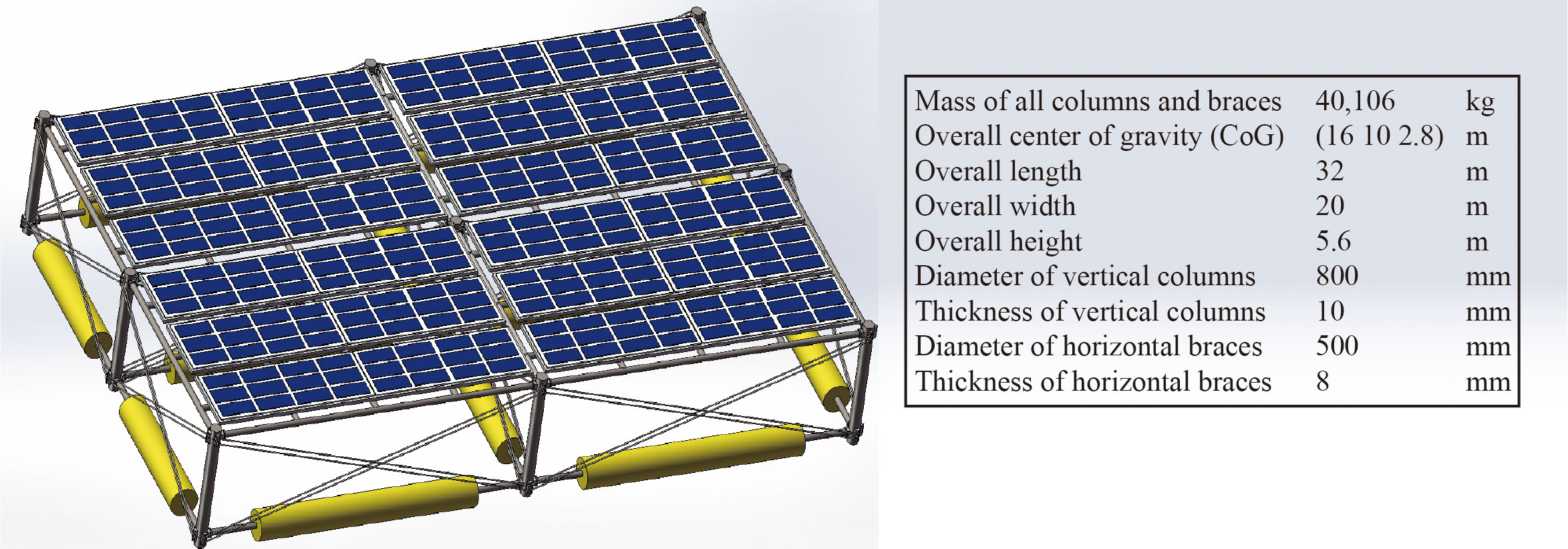
Figure 1 The offshore FPV with single floater and its structural properties.

The demand of offshore FPVs has been expanding due to the CO₂ emission requirement of each country, such as Japan, South Korea, Netherlands, UK, Norway, China and India. However, the past research mainly focused on inland PVs. The lack of specific design standards is attributed to the low maturity of offshore FPV technology. In fact, the operation environment of offshore FPVs is much severer than in lakes or rivers where inland FPVs are located. Standards and guidelines to verify different limit state, including ultimate, fatigue, service and accidental, should be established by classification societies or government associations to accelerate the growth of offshore FPVs’ market. Among all limit states, fatigue damage is regarded as one big technical challenging. Due to the low manufacture budget of FPVs, its strength cannot be designed as high as other offshore structures. In addition, the lifetime of offshore FPVs is commonly designed as 25 years. The dynamic wind and wave loads may easily accumulate fatigue cracks at the structures’ joint and connection spots.

2.2 Fatigue assessment

Different from inland PVs, offshore FPVs are exposed to marine environment and subjected to wind, wave and current. Among them, waves are the primary source of fatigue damage (Paik and Thayamballi, 2007), because wave loadings are producing fluctuating stress in structures, which result in cumulated fatigue damage. Fatigue assessment is important to FPVs, because fatigue failure can even occur under cyclic loadings below ultimate limit states. Hence, in design stage, it is highly recommended to identify all the wave conditions which the FPV will encounter in their service life.

In fatigue assessment, sea states are defined as the statistical description of wave conditions over 3 or 6 hours. According to classification notes (DNV, 2014), sea states in fatigue design are represented by wave scatter diagrams. Each block in the scatter diagram stands for one sea state with its significant wave height $H_s$), zero crossing period ($T_z$) and occurrence. The sea states in scatter diagrams are characterized based on observations, measurements or hindcast.

It is believed that these sea states in scatter diagrams still need further improvement since they are all from observations and measurements in the past (Zou and Kaminski, 2016; Zou and Kaminski, 2020). It is assumed that past sea states can be representative of future sea states. The lifecycle of FPVs may be as long as 25 years. The wave conditions measured in the past may not necessarily be representative of the future wave conditions that FPVs will encounter in their service life. There might be decades passed between the wave observations and the service of offshore structures. And the sea states in the future will probably become significantly different from the sea states in the past (Bitner-Gregersen and Eide, 2010). Therefore, it is necessary to update the scatter diagrams with the consideration of climate change impact.

According to finite element analysis and experience, the tubular joints of FPVs are the most sensitive spots for fatigue damage. The varying stresses in joints initiate fatigue cracks, and these cracks when propagating may subsequently cause a fatigue failure.

For offshore structures, fatigue damage is usually calculated based on the spectral approach, and the fatigue resistance is represented by S-N curves (DNV, 2014). If the long-term stress range distribution is defined as the sum of the Rayleigh distribution of each short term stress range corresponding to each sea state, the cumulative fatigue damage with one slope S-N curve is given by:

$\begin{array}{ll}\text{D}=\frac{{\omega }_0{T}_d}{a}\Gamma \left(1+\frac{m}{2}\right){\displaystyle {\sum }_{n=1}^{N_{load}}{p}_n}{\displaystyle {\sum }_{i=1,j=1}^{\begin{array}{c}\mathit{\text{all seastates}}\\ \mathit{\text{all headings}}\end{array}}{r}_{ijn}}{(2\sqrt{2m_{0ijn}})}^m& \text{(2.1)}\end{array}$

where D is accumulated fatigue damage, ${\omega }_0$ is the average long-term zero-crossing frequency, a and m are the S-N curve parameters, $T_d$ is the design life of offshore structures $\Gamma$ is gamma function, $N_{load}$ is total number of load conditions, $p_n$ is the fraction of design life in load condition $n$, $r_{ijn}$ is relative number of stress cycles in short-term condition $i,j$, $m_{0ijn}$ is zero spectral moment of stress response process.

The stress response spectrum and spectral moments in linear models are defined as

$\begin{array}{ll}{S}_{\sigma }(\omega |H_s, T_z,\theta )={\left|H_{\sigma }(\omega |\theta )\right|}^2·S_{\eta }(\omega |H_s, T_z)& \text{(2.2)}\end{array}$

$\begin{array}{ll}{m}_n={\int }_{\omega }{\displaystyle {\sum }_{\theta -{90}^{°}}^{\theta +{90}^{°}}f(\theta ){\omega }^n}·S_{\sigma }(\omega |H_s, T_z,\theta )d\omega & \text{(2.3)}\end{array}$

where $H_{\sigma }(\omega |\theta )$ is the transfer function which represent the relation between unit wave amplitude and response, $S_{\eta }(\omega |H_s, T_z)$ is wave spectrum, $f(\theta )$ is the wave spreading function. It can be seen that, for a particular offshore structure, the fatigue damage is mainly determined by sea states which are represented by wave scatter diagrams or time series of sea states.

2.3 Numerical simulations

A fully coupled simulation is conducted for dynamic analysis in the time domain of the FPVs, see Figure 2. A preprocessor GeniE software is used for the structural modelling with tubular beam elements, and the model is then transferred to HydroD for hydrodynamic analysis. HydroD is a program to analyze the global response of floaters. WADAM is one module of HydroD for frequency domain analysis. The kinetic parameters including hydrostatic data, wave force transfer function and so on are obtained from HydroD and outputted into SIMA for further analysis. SIMA software include SIMO and RIFLEX programs. SIMO calculates the aerodynamic and hydrodynamic loads on the FPV structure. Since the FPVs are modelled as a rigid body, the aerodynamic loads on them are simplified to calculate based on Equation 2.4. The hydrodynamic loads mainly include first-order wave loads, second-order wave drift loads, and viscous drag force. They are calculated respectively based on the linear potential flow theory, the Newman’s approximation, the viscous term of the Morison equation and quadratic drag force coefficient. RIFLEX models the mooring lines of FPVs. With SIMO and RIFLEX, a time domain dynamic analysis is conducted and the structural response of FPVs in each sea state is simulated. Then, the output is transferred into ANSYS for local analysis.

FIGURE 2

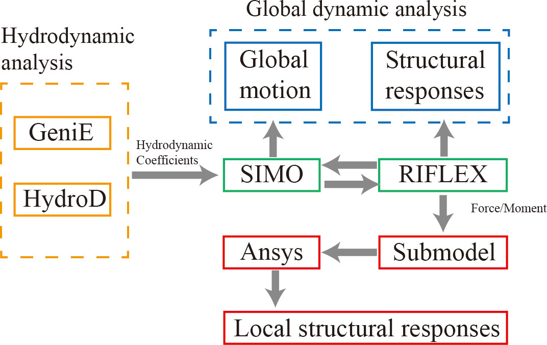
Figure 2 Flow chart of numerical simulations.

$\begin{array}{ll}q=\text{C}(\text{α})v^2& \text{(2.4)}\end{array}$

$q$ is wind force; $\text{C}(\text{α})$ is wind force coefficient for the instantaneous relative direction $\text{α}$, and $v$ is relative wind speed between body and wind. After an initial verification of the convergence tests, the validation of this fully coupled simulation method has been conducted through a model-to-experiment comparison for floating offshore wind turbines from (Zou et al., 2021). In the future study of optimization with increasing complexity of the FPV structures, a multiple FPV array instead of a single floater is planned to be examined through experiments which would provide solid experimental data to further validate the numerical simulation method for complex FPVs.

3 Climate change impact

Climate change is a long-term cumulative process, and it changes the wave conditions slowly and gradually. The lifecycle of a FPV may be over 25 years in length, and the annual fatigue damage is probably influenced where wave conditions are sensitive to climate change. The relations between climate change and fatigue damage are clarified in Figure 3 from a physical point of view.

● Due to natural variability and human-induced climate change (greenhouse gases emission), the climate circulation is changed. The atmosphere makes the most rapid response to climate change. The surface wind field, as the part of lower atmosphere, is circulating differently.

● Most ocean surface waves are generated by wind. Therefore, the climate change leads to different wave conditions.

● The waves are the primary source of fatigue damage for offshore floating structures. As a result, fatigue damage may be affected by wave changes.

FIGURE 3

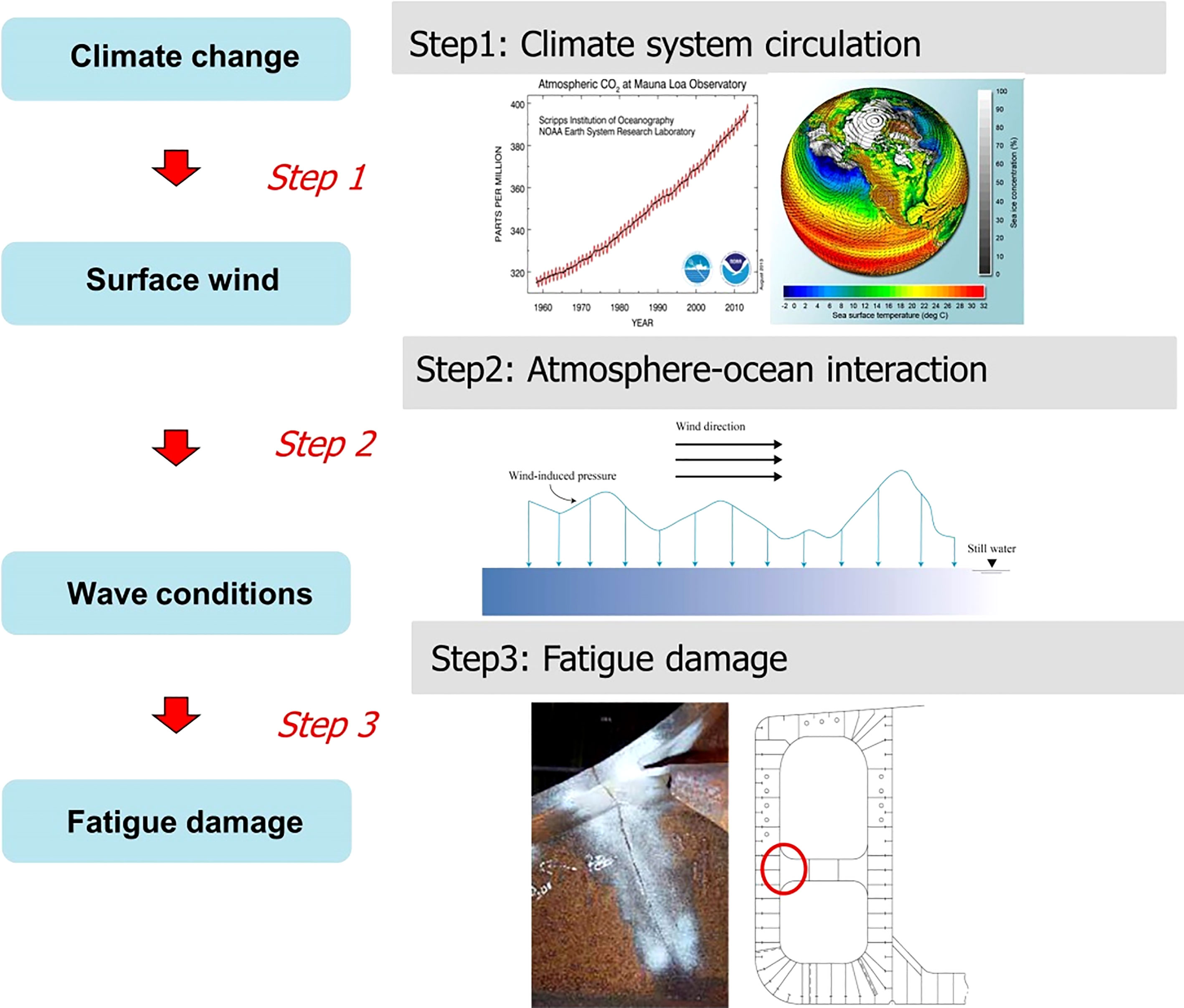
Figure 3 The relation between climate change and fatigue damage from a physical point of view.

3.1 Global climate models and climate scenarios

The modelling technology of the climate system has been highly developed since last century. In 1995, the Coupled Model Intercomparison Project (CMIP) was proposed to better understand past, present and future climate changes arising from natural, unforced variability or in response to changes in radiative forcing in a multi-model context. In 2014, its sixth phase (CMIP6) was initiated with the aim to fill scientific gaps remaining in CMIP5 and address new challenges emerging in climate modeling (Taylor et al., 2012). Tens of global climate models (GCMs) are constructed by the fundamental physical laws (such as conservation of mass, energy and momentum) with many specific developments in CMIP (Solomon et al., 2007).

These models were designed to simulate the circulation of climate system for different specific purposes and may differ in parametrizations and numerical formulations. GCMs usually include atmospheric and ocean components. According to their design objective, some of them also include sea ice and land components as shown in Figure 4 (Wu et al., 2014). Many factors may affect the radiative forcing. For offshore engineering, more attentions should be paid on the emission of greenhouse gases (GHGs), because the greenhouse effect has a shorter time-scale (from decades to centuries). As there is a range of climate models in CMIP6, it is hardly possible to give a detailed description of all these models. The following part of this section focuses on the atmosphere model, because it is the key component in this study.

FIGURE 4

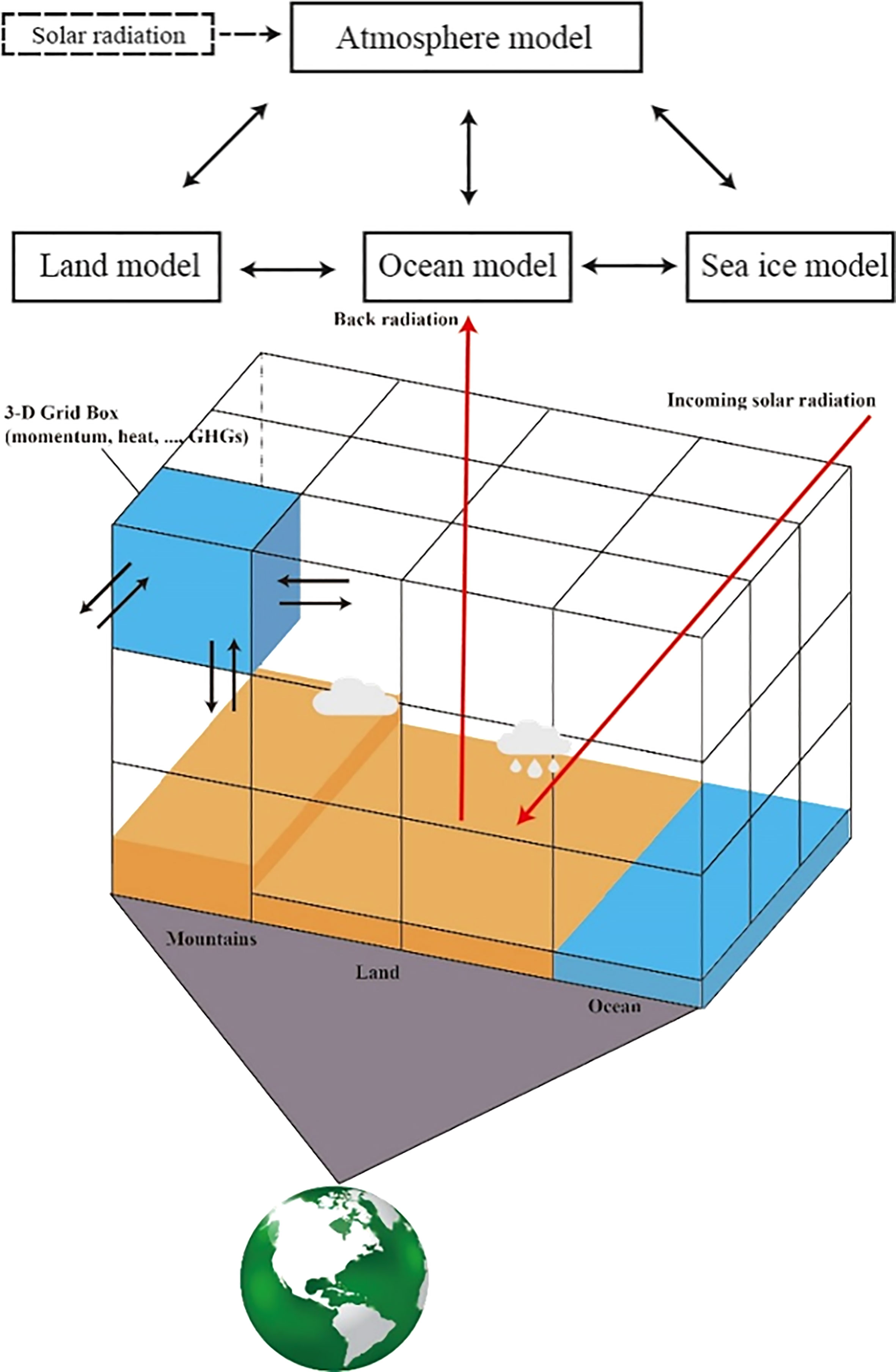
Figure 4 Climate component models. There are four climate components in the climate system. The emission of greenhouse gases affects the solar radiation and results in the climate change.

Climate scenarios are used to describe the historical and future climate with respect to a wide range of variables including socio-economic change, technological development, energy composition, land use, and emissions of GHGs and air pollutants (van Vuuren et al., 2011). A group of climate scenarios named as “Shared Socioeconomic Pathways” (SSPs) were initially developed since 2016, see Figure 5. These climate scenarios consider factors such as population, economic growth, education, urbanization and the rate of technological development at five different ways in which the world might evolve in the absence of climate policy. SSPs provide the trajectories of all the radiative forcing components over time, including the emissions of GHGs, air pollutants, and land use. The trajectories cover both the historical and future period from 2015 to 2100, and all the RCPs have been harmonized for a smooth transition between the historical and future periods. Some researchers even further extended the time period covered by SSPs to 2500 (Meinshausen et al., 2020).

FIGURE 5

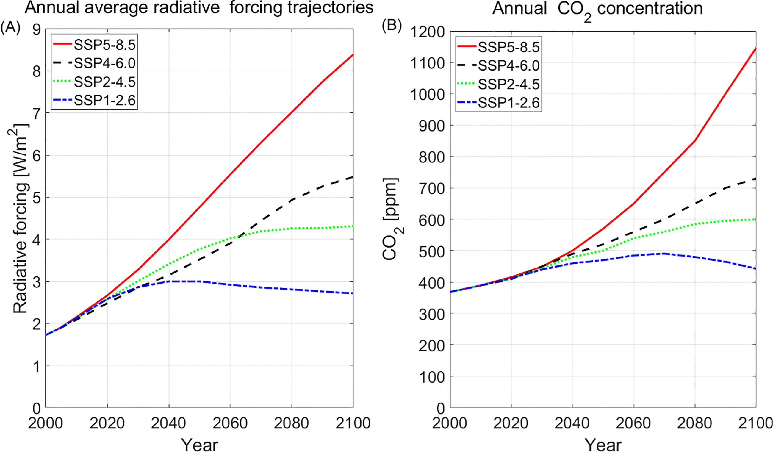
Figure 5 (A) Radiative forcing and (B) CO2 concentration trajectories of SSPs. The climate data before 2015 are from Representative Concentration Pathways (RCPs) and historical data.

3.2 Wind-driven wave models

Most ocean waves are generated by surface winds. With climate models, the atmospheric circulation in each layer is numerically simulated. The surface wind field, as part of the lower layer of atmosphere, is also modelled. Then, in order to describe the evolution of wave spectrum in each sea state, wind-driven wave models are designed to numerically simulate wind-wave interactions, nonlinear wave-wave interactions, and energy dissipation over a large or even global scale (Janssen, 2008). The driving force of wave models is the surface wind field. By coupling climate models to wave models, it is feasible to simulate the climate change impact on ocean waves. In other words, the response of ocean surface to climate scenarios (i.g., ocean waves) can be simulated by wave models. If the radiative forcing is changed, the wave simulations would also be affected.

The wave conditions are represented by wave spectra in wave modelling. The most widely used wind-driven wave models are Ocean Wave Model (WAM) (Komen et al., 1996), Simulating WAves Nearshore model (SWAN) (Booij et al., 1996), and WaveWatch-III (WW3) model (Tolman and the WAVEWATCH III Development Group, 2014). These models have been widely applied in coastal engineering (Booij et al., 1999), wave energy harvesting (Rusu and Soares, 2009), wave forecasting and hindcasting (Gómez Lahoz and Carretero Albiach, 2005). All these wave models are constructed based on energy conservations. The wave spectra over a sea area are simultaneously calculated on Cartesian x,y-grids (the Eulerian approach), as demonstrated in Figure 6.

FIGURE 6

Figure 6 The energy propagation through one cell of the grid.

In an idealized case where a constant wind (constant in space and time) is blowing over deep open water, the wave energy is locally balanced for each cell as:

$$\begin{array}{c}\mathit{\text{change of energy in cell}}\\ =\mathit{\text{net import of energy}}+\mathit{\text{local generation of energy}}\end{array}$$

Since the group wave speed in deep water is independent of geographical locations, the spectral energy balance equation is as follows:

$\begin{array}{ll}\frac{\partial E\mathbf{(}k,\theta ;x,y,t\mathbf{)}}{\partial t}+c_{g,x}\frac{\partial E\mathbf{(}k,\theta ;x,y,t\mathbf{)}}{\partial x}+c_{g,y}\frac{\partial E\mathbf{(}k,\theta ;x,y,t\mathbf{)}}{\partial y}=S\mathbf{(}k,\theta ;x,y,t\mathbf{)}& \text{(3.1)}\end{array}$

In marine environment, ocean currents may also affect wave energy balance and make it no longer conserved. In contrast, wave action N $(k,\theta ;X,t)=\text{E}(k,\theta ;X,t)/\text{σ}$ is still conserved (Whitham, 1965; Bretherthon and Raymond Garrett, 1968). If we consider the influence of ocean current $U$, the energy balance equation should be transferred into the spectral action balance equation as:

$\begin{array}{ll}\frac{\partial N}{\partial t}+{\nabla }_x·\dot{X}N+\frac{\partial }{\partial k}\dot{k}N+\frac{\partial }{\partial \theta }\dot{\theta }N=\frac{S}{\sigma }& \text{(3.2)}\end{array}$

$\begin{array}{ll}\dot{X}=c_g+U& \text{(3.3)}\end{array}$

$\begin{array}{ll}\dot{k}=-\frac{\partial \sigma }{\partial d}\frac{\partial d}{\partial s}-k·\frac{\partial U}{\partial s}& \text{(3.4)}\end{array}$

$\begin{array}{ll}\dot{\theta }=-\frac{1}{k}[\frac{\partial \sigma }{\partial d}\frac{\partial d}{\partial r}+k·\frac{\partial U}{\partial r}]& \text{(3.5)}\end{array}$

$\begin{array}{ll}S=S_{in}+S_{nl}+S_{ds}+S_{bot}+S_{db}& \text{(3.6)}\end{array}$

where $\text{N}(k,\theta ;X,t)$ is the wave action density spectrum, $\text{N}(k,\theta ;X,t)=\text{E}(k,\theta ;X,t)/\text{σ}$, $\text{E}(k,\theta ;X,t)$ is wave variance spectrum, X stands for the geographical variables (x, y in Cartesian grids or λ, φ in longitude-latitude grids), $\sigma$ is radian frequency, $U$ and $c_g$ are the vectors of current and wave group given by group speed $c_g$ and wave direction $\text{θ}$, $k$ is wave number vector, $d$ is mean water depth, $\text{s}$ is a coordinate in the direction $\text{θ}$, and $\text{r}$ is a coordinate perpendicular to $s$. $S$ is the source function. In deep water, the source function includes three parts: wind-wave generation ($S_{in}$), nonlinear wave-wave interaction ($S_{nl}$) and dissipation by wave breaking ($S_{ds}$). In shallow water, wave-bottom interactions ($S_{bot}$) and depth-induced breaking ($S_{db}$) are also considered.

3.3 Global time step and grid sensitivity

Spatial resolutions and time steps are two key parameters in wave model simulations. In order to investigate the sensitivity of fatigue damage to them, wave conditions were simulated by coupling WaveWatch-III wave model to ERA-Interim reanalysis data with different grid sizes (0.25°×0.25°,0.75°×0.75°,1.25°×1.25°,1.50°×1.50° Lat/Lon) and time step settings. Fatigue damage at the midship of a FPSO (Floating Production Storage and Offloading) named Glas-Dowr was calculated based on different scatter diagrams. The first five scatter diagrams were generated with the same grid size (0.75°×0.75° Lat/Lon) but different global time step settings. Another four scatter diagrams were made with the same time step setting (the global time step is 3600s) but different grid sizes. The results of fatigue calculations were compared in Figure 7.

FIGURE 7

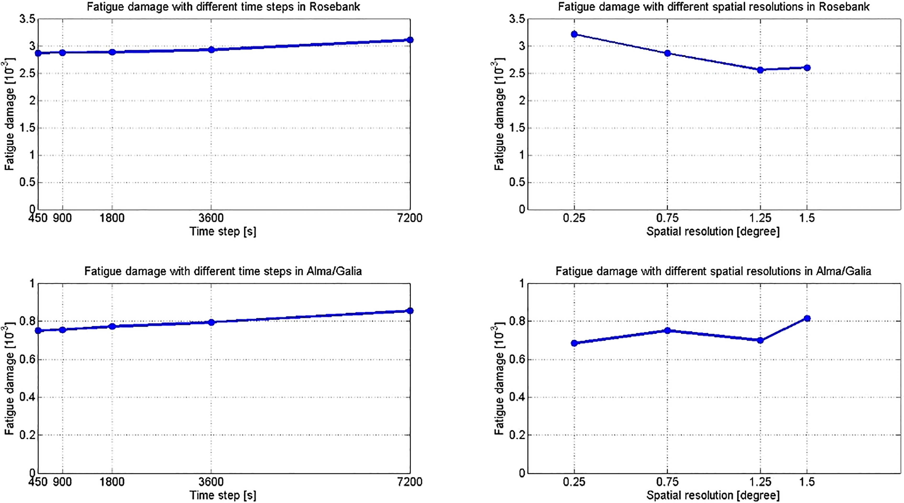
Figure 7 Global time step and grid sensitivity analysis.

4 Case study in the North Sea

The North Sea is a mature oil and gas producing region. In the meanwhile, plenty of floating solar farms have been installed in the North Sea during recent years. Most FPVs are located near coastal area to minimize the electrical transmission cost, and some other FPVs are designed to located near offshore oil fields to support power. In this case study, three North Sea oil fields were selected, Rosebank, Alma and Pierce, see Figure 8A. The oil fields Alma (56.2°N; 2.8°E) and Pierce (58°N; 1.45°E) are both in the central North Sea with a water depth of approximately 100 meters. Rosebank oil field (61°N; 4°W) is located North-West of the Shetland Islands with a water depth of approximately 1100 meters. FPVs are located in these oil fields to supply electricity to offshore platforms, as shown in Figure 8B. The floater is moored with four catenary lines spread symmetrically about the X-axis and Y-axis. The fairleads are located at the bottom of the floater. Each of these four lines has an unstretched length of 410m and a diameter of 0.0766m. The submerged equivalent mass per unit length is 108.63 kg/m, and the equivalent extensional stiffness is set as 753.6 MN. The structural properties of FPVs are listed in Figure 1. Based on the projection method, this case study aims to evaluate the sea states in three time period 2011-2020, 2051-2060, 2091-2100 with a high GHG emission climate scenario. Then, the trend of annual fatigue damage is calculated in section 4.2.

FIGURE 8

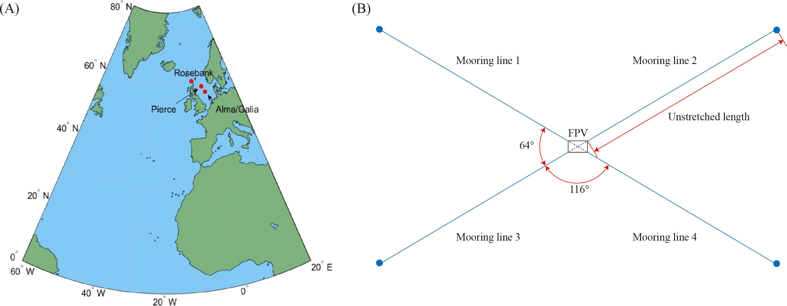
Figure 8 (A) Geographical locations of three fields in the North Sea. The wave modelling area covers a region of 0°-80°N/60°W-20°E Latitude/Longitude. (B) The mooring lines of floaters.

4.1 Sea states projection

A large scale of wave simulation is required to simulate all the waves in the North Sea to consider the waves from nearby sea areas, as shown in Figure 8A. A rectangular region of 70°S-60°N/70°W-120°E Latitude/Longitude were simulated by WaveWatch-III Version 6.07. The wave-driving forces were from five GCMs: ACCESS-ESM1, CMCC-ESM2, CanESM5, CNRM-CM-6-1 and IPSL-CM6A-LR. This semi-global simulation can ensure that all the swells generated in remote sea areas could propagate into the North Sea. Each 6-hourly wave condition was represented by a multi peak JONSWAP wave spectrum defined for 24 directions (i.e. every 15°) and 25 frequencies ranging from 0.042 Hz to 0.414 Hz. The spatial resolution of grids in the model is 0.75°×0.75° Latitude/Longitude with the global time step 3600 seconds. More details of the wave simulations are listed in Table 1. By coupling global climate models to wave models, the continuous wave conditions of 30 years (2011-2020, 2051-2060, 2091-2100) are projected and simulated. The 30 years wave conditions include $30yr\times 365days\times 4=43800$ 6-hour sea states. It will be very time-consuming to make the simulations for each sea state. Instead, a spectral fatigue calculation method is used from DNV (2014) to simplify the calculation process. The spectral fatigue calculations are based on stress transfer functions established through SIMO/Riflex numerical simulations. This spectral method assumes linear load effects and responses, and the nonlinear effect is neglected. Then, a wave scatter diagram is created by these 30 years wave conditions, and the fatigue damage is calculated with the stress response spectrum. The stress response spectrum and spectral moments in linear models are defined as

TABLE 1

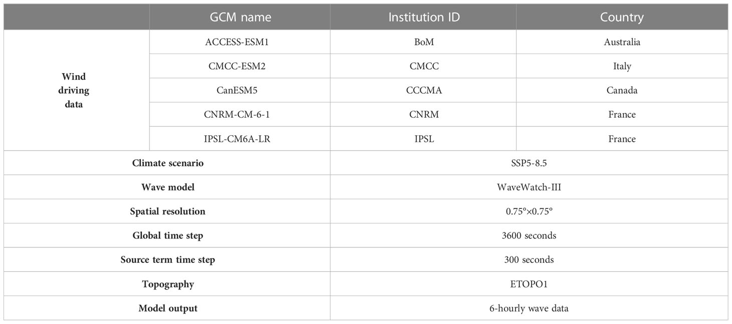
Table 1 The wave modelling details.

$\begin{array}{ll}{S}_{\sigma }(\omega |H_s, T_z,\theta )={\left|H_{\sigma }(\omega |\theta )\right|}^2·S_{\eta }(\omega |H_s, T_z)& \text{(4.1)}\end{array}$

$\begin{array}{ll}{m}_n={\int }_{\omega }{\sum }_{\theta -{90}^{°}}^{\theta +{90}^{°}}f(\theta ){\omega }^n·S_{\sigma }(\omega |H_s, T_z,\theta )d\omega & \text{(4.2)}\end{array}$

where $H_{\sigma }(\omega |\theta )$ is the transfer function which represent the relation between unit wave amplitude and response, $S_{\eta }(\omega |H_s, T_z)$ is wave spectrum, $f(\theta )$ is the wave spreading function.

4.2 Annual fatigue damage projection

Although wave scatter diagrams are recommended for fatigue analysis by many classification societies (DNVGL, 2016; DNVGL, 2018), they are not exactly representative of ocean waves due to the impact of climate change. In addition, some important information of wave properties is limited when constructing scatter diagrams, such as wave directions, wave directional spreading and the sequence of sea states. In this section, the wave scatter diagrams in those three oil fields are upgraded with the sea states data projected by the wind-driven wave model WaveWatch-III. The output of WaveWatch-III is exemplified in Table 2, including wave properties such as significant wave height (H_s), zero crossing period (T_z), mean wave direction (θ), and directional spreading coefficient (s) for each wave system (wind waves and swells). The fatigue damage is calculated with each wave system independently. Then, the total fatigue is the sum of them. A multi peak JONSWAP wave spectrum is used here to represent the wave systems.

TABLE 2

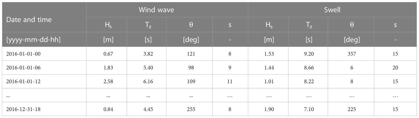
Table 2 An example of sea state time-series from WaveWatch-III.

For fatigue assessment, a global-local methodology of the fatigue calculation procedure is utilized, emphasizing the theoretical concepts associated with the submodelling and fatigue methods (Zou et al., 2022). A general workflow for the global-local fatigue assessment methodology is suggested in Figure 9, introducing two different phases of analysis that follow an increasing detail of geometrical, material and contact properties as the assessment progresses from the global to the local scale. The two fatigue analysis phases are systematized as follows.

FIGURE 9

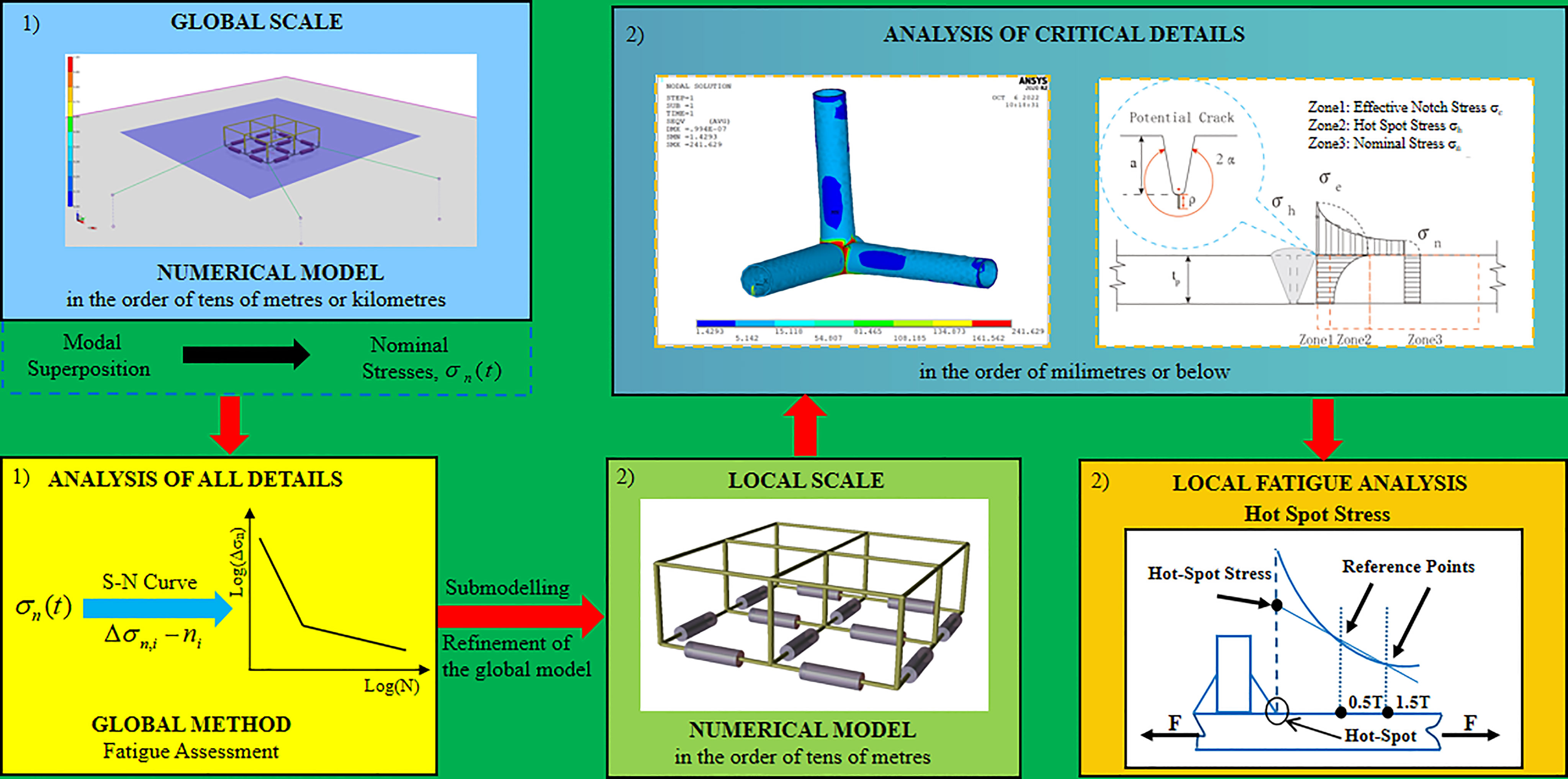
Figure 9 Workflow of the global-local fatigue assessment methodology.

In the first phase, a global approach based on the accumulation of damage computed with nominal stresses and S-N curves is used. The global finite element model of FPV was created by a Sesam module GeniE, see Figure 10B. A time domain dynamic analysis of FPVs’ response, including motions and sectional loading, is conducted through SIMO and RIFLEX, see Figure 10A. Then, SIMO simulates the response of rigid bodies in the time domain based on a frequency domain analysis by WADAM. The hydrodynamic forces on the FPV are calculated based on Morison equations with the hydrostatic coefficients from WADAM. The global numerical model should be accurate enough to obtain nominal stresses to be used as input loading for the linear damage accumulation method. Nonetheless, the available S-N curves with nominal stress may not properly reflect the local geometrical and material characteristics of critical details, and conservative assessment for the fatigue resistance may be considered. Based on this fatigue analysis result, the critical details should be identified which require a more refined assessment by implementing local scale models.

FIGURE 10

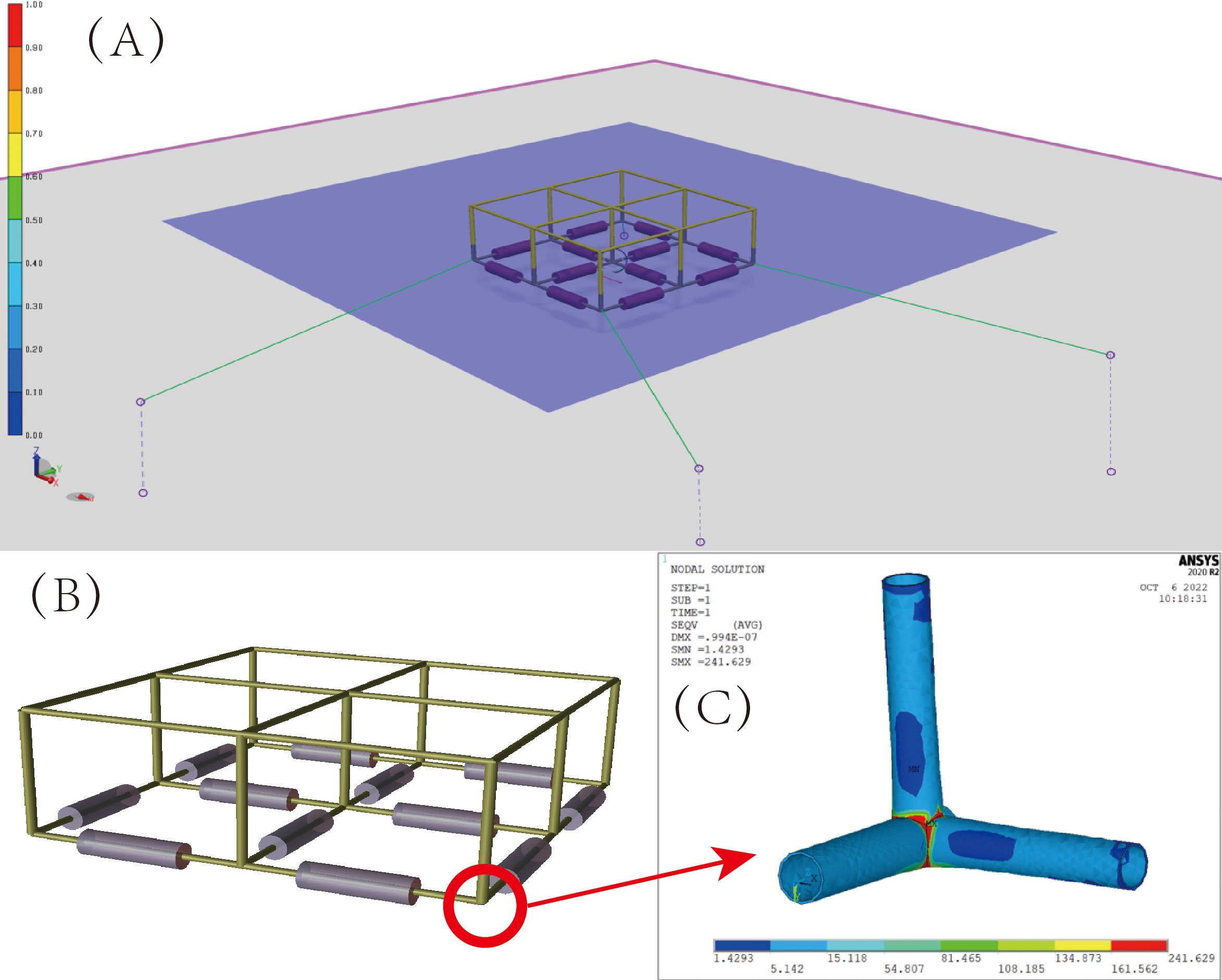
Figure 10 (A) The time domain dynamic model of FPVs; (B) The GeniE global model of FPVs; (C)The local model of FPVs’ joint.

In the second phase, submodelling techniques are used to evaluate accurately local fatigue damage. The local FE model of a tubular joint was created. are shown in Figure 10C, because there is a high stress concentration due to its irregular geometry. The hot spot stress approach evaluates the fatigue damage with the projected sea states from WaveWatch-III. After a convergence study, the mesh size is chosen as minimum 0.9 mm and maximum 16mm. The areas near the weld joints are meshed with smaller mesh size to improve the accuracy. The one-slope S-N curve with m=3 and log(C) =12.44 (stress in MPa) is recommended by DNV to represent the fatigue resistance of steel material in a corrosive environment (DNV, 2014). Recommended stress evaluation points are located at distances t/2 and 3t/2 away from the hot spot, where t is the plate thickness at the weld toe (DNV, 2014).

5 Discussion

With the wind driving force from GCMs, the sea states in the North Atlantic were projected by WaveWatch-III. Then, the annual $H_s$ in the selected oil fields were calculated. There is a downward trend of annual $H_s$ over time in all three oil fields as shown in Figure 11. The $H_s$ decreased by approximately 0.5 meter from 2011 to 2100. Considering that the North Sea is a wind-wave-dominated sea area, this decrease is in agreement with the earlier findings (Young et al., 2011; Dobrynin et al., 2015). These earlier findings reveal that the overall wind speed in the North Sea is decreasing with the emission of GHGs over time. Furthermore, the results indicate that the averaged wave height of Rosebank oil field under projected simulations is higher than the other oil fields. As the distance between Alma/Galia and Pierce oil fields is not far, their averaged wave heights are relatively close to each other, as listed in Table 3. Rosebank has the highest wave height, because it is also vulnerable to waves from the Atlantic Ocean.

FIGURE 11

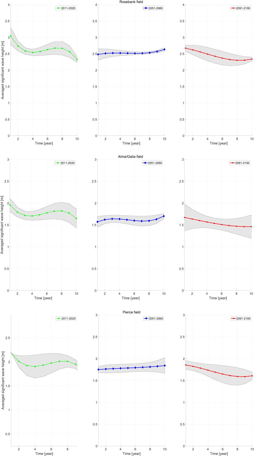
Figure 11 Projections of significant wave height at the selected oil fields with five GCMs.

TABLE 3

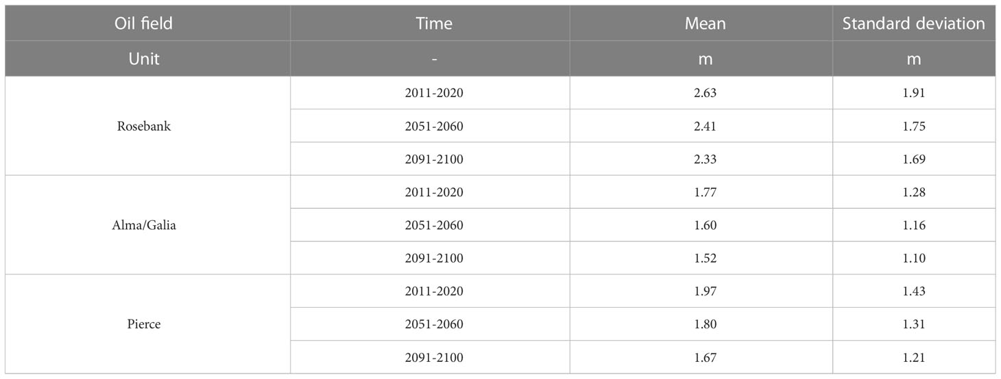
Table 3 Statistical characteristics of significant wave height under the projected simulations.

The annual fatigue damages in the oil fields of North Sea were also calculated using the sea states from projected simulations. All these three oil fields show a decreasing trend of annual fatigue damage over time as shown in Table 4. This trend is consistent with the trend of significant wave height. Based on the similar trends in these three oil fields, it is concluded that the sea states in the North Sea is becoming milder and the annual fatigue damage is decreasing. The sea states in Rosebank is the severest, which result in the highest fatigue damage. The fatigue damages in the other two fields are much lower, because they are not vulnerable to the swells from the North Atlantic. The fatigue lifetime of FPVs is growing due to the climate change impact. In Rosebank, the fatigue lifetime of FPVs is as long as 36 years based on the sea states in 2011-2020. According to the projections, the lifetime is extended to by 14% to 41 years based on the sea states in 2051-2060, and further extended to 49 at the end of this century. In the other two oil fields, the impact of climate change on fatigue damage is not so significant.

TABLE 4

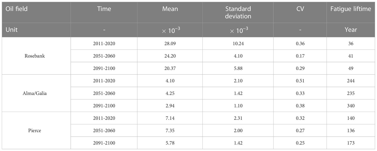
Table 4 Projection of annual fatigue damage in three oil fields.

Generally, their annual fatigue damage is decreasing and fatigue lifetime is growing longer, but this trend is not so consistent and as clear as in Rosebank. Their difference of climate change impact in these three oil field is also attributed to the geographic locations. The climate change has a stronger impact on the swells from the Atlantic Ocean, which result in a more significant trend of annual fatigue damage in Rosebank. Hence, the composition of mixed waves (the proportion of wind waves and swells) is dependent on the location. The climate change is affecting wind waves and swells in different ways. Different compositions may affect the amount of climate change impact. It is highly recommended to partition the wave spectra into multiple wave systems (normally, one wind wave and several swells) to evaluate the climate change impact on each wave system individually, and to improve the reliability of fatigue assessment.

6 Conclusions

This study presented a projection method to evaluate the climate change impact on fatigue damage of offshore FPVs in the future. A case study was demonstrated in the North Sea. By coupling the global climate models to wind-driven wave models, the wave conditions in a large-scale sea area were simulated. Then, with the specific climate scenario, the sea states in 2011-2020, 2051-2060 and 2091-2100 were projected. At last, the fatigue assessment on a FPV’s joint was conducted for these three periods. The main conclusions are as follows:

1. The case study confirms that there is a clear decreasing trend of significant wave height with the high emission of GHGs. The significant wave height declines by 11%-15% in the North Sea from 2011-2100. But the decreasing rates are not equal in these three oil fields (Rosebank, Alma and Pierce). The rate of wave change is region dependent, because ocean waves consist of wind waves and swells. The climate change is affecting wind waves and swells in different ways. To improve the evaluation of climate change impact on waves, it is recommended to partition waves into multiple wave systems. For example, the North Sea is dominated by wind waves. The study on the change of wind waves in the North Sea is more important than on swells.

2. Although the wave height is the dominant wave characteristic in fatigue calculations, fatigue damage is also affected by the change of other wave characteristics. In the fatigue assessment, the one-slope S-N curve is selected with m=3. In a linear model, the fatigue loads are proportional to Hs³, when all other wave parameters are unchanged. If Hs decreases by 11%-15%, the annual fatigue damage should decline by 30%-39%. However, according to the result of fatigue assessment, the annual fatigue damage is only reduced by 19%-28% from 2011-2100. This difference is mainly induced by the change of other wave parameters such as wave period. As a result, fatigue trends are not so significant as wave height trends in the North Sea.

3. The fatigue assessment shows that with the emission of CO2, the annual fatigue damage is decreasing, especially in the Rosebank field. The fatigue lifetime is extended from 36 years to 49 years. It can be concluded that the FPVs designed based on the sea states in the past will be conservative in the near future. It indicates the fatigue strength requirement for FPVs in the North Sea will be lowered. The manufacture cost of FPVs can be reduced to some extent, which is beneficial to the commercial market.

Data availability statement

The raw data supporting the conclusions of this article will be made available by the authors, without undue reservation.

Author contributions

TZ: Writing - original draft, conceptualization, methodology. XB: Visualization, data curation. XJ: Software, visualization. XC: Validation. LT: Supervision. All authors contributed to the article and approved the submitted version.

Funding

This research is supported by the Shandong Provincial Key Laboratory of Ocean Engineering with grant No. kloe202010, the Natural Science Foundation of Jiangsu Province (Grant No. BK20220654, BK20190962) and the National Natural Science Foundation of China (Grant No. 52001144). The authors would like to thank the Key R & D Projects in Guangdong Province (No. 2020B1111500001) for their financial supports.

Conflict of interest

The authors declare that the research was conducted in the absence of any commercial or financial relationships that could be construed as a potential conflict of interest.

The reviewer XX declared a shared affiliation with the authors TZ, XN, XJ.

Publisher’s note

All claims expressed in this article are solely those of the authors and do not necessarily represent those of their affiliated organizations, or those of the publisher, the editors and the reviewers. Any product that may be evaluated in this article, or claim that may be made by its manufacturer, is not guaranteed or endorsed by the publisher.

References

Bitner-Gregersen E., Eide L. (2010). Climate change and effect on marine structure design Vol. 1 (Oslo, Norway: DNVRI Position Paper).

Google Scholar

Bitner-Gregersen E. M., Vanem E., Gramstad O., Hørte T., Aarnes O. J., Reistad M., et al. (2018). Climate change and safe design of ship structures. Ocean Eng. 149, 226–237. doi: 10.1016/j.oceaneng.2017.12.023

CrossRef Full Text | Google Scholar

Booij N., Holthuijsen L. H., Ris R. C. (1996). The SWAN wave model for shallow water (Orlando, USA: Coastal Engineering).

Google Scholar

Booij N., Ris R., Holthuijsen L. H. (1999). A third-generation wave model for coastal regions: 1. model description and validation. J. geophys. res.: Oceans 104 (C4), 7649–7666.

Google Scholar

Bretherthon F. P., Raymond Garrett C. J. (1968). Wavetrains in inhomogeneous moving media. Proc. R. Soc. London Ser. A Math. Phys. Sci. 302 (1471), 529–554.

Google Scholar

Claus R., López M. (2022). Key issues in the design of floating photovoltaic structures for the marine environment. Renewable Sustain. Energy Rev. 164, 112502. doi: 10.1016/j.rser.2022.112502

CrossRef Full Text | Google Scholar

DNV (2014). Fatigue assessment of ship structures.

Google Scholar

DNVGL (2016). Design of offshore steel structures. General-LRFD Method.

Google Scholar

DNVGL (2018). Support structures for wind turbines.

Google Scholar

Dobrynin M., Murawski J., Baehr J., Ilyina T. (2015). Detection and attribution of climate change signal in ocean wind waves. J. Climate. 28 (4), 1578–1591. doi: 10.1175/JCLI-D-13-00664.1

CrossRef Full Text | Google Scholar

Gao J., Ma X., Dong G., Chen H., Liu Q., Zang J. (2021). Investigation on the effects of Bragg reflection on harbor oscillations. Coast. Eng. 170, 103977. doi: 10.1016/j.coastaleng.2021.103977

CrossRef Full Text | Google Scholar

Gao J., Ma X., Zang J., Dong G., Ma X., Zhu Y., et al. (2020). Numerical investigation of harbor oscillations induced by focused transient wave groups. Coast. Eng. 158, 103670. doi: 10.1016/j.coastaleng.2020.103670

CrossRef Full Text | Google Scholar

Gómez Lahoz M., Carretero Albiach J. (2005). Wave forecasting at the Spanish coasts. J. Atmos. Ocean Sci. 10 (4), 389–405. doi: 10.1080/17417530601127522

CrossRef Full Text | Google Scholar

Hemer M. A., Fan Y., Mori N., Semedo A., Wang X. L. (2013). Projected changes in wave climate from a multi-model ensemble. Nat. Climate Change. 3 (5), 471–476. doi: 10.1038/nclimate1791

CrossRef Full Text | Google Scholar

Hooper T., Armstrong A., Vlaswinkel B. (2021). Environmental impacts and benefits of marine floating solar. Solar Energy. 219, 11–14. doi: 10.1016/j.solener.2020.10.010

CrossRef Full Text | Google Scholar

Janssen P. A. E. M. (2008). Progress in ocean wave forecasting. J. Comput. Phys. 227 (7), 3572–3594. doi: 10.1016/j.jcp.2007.04.029

CrossRef Full Text | Google Scholar

Komen G. J., Cavaleri L., Donelan M., Hasselmann K., Hasselmann S., Janssen P. (1996). Dynamics and modelling of ocean waves (Cambridge, UK: Cambridge university press).

Google Scholar

Liu H., Krishna V., Lun Leung J., Reindl T., Zhao L. (2018). Field experience and performance analysis of floating PV technologies in the tropics. Prog. Photovoltaics: Res. Applications. 26 (12), 957–967. doi: 10.1002/pip.3039

CrossRef Full Text | Google Scholar

Meinshausen M., Nicholls Z. R. J., Lewis J., Gidden M. J., Vogel E., Freund M., et al. (2020). The shared socio-economic pathway (SSP) greenhouse gas concentrations and their extensions to 2500. Geosci. Model. Dev. 13 (8), 3571–3605. doi: 10.5194/gmd-13-3571-2020

CrossRef Full Text | Google Scholar

Paik J. K., Thayamballi A. K. (2007). Ship-shaped offshore installations: design, building, and operation (Noew York, US: Cambridge University Press).

Google Scholar

Rosa-Clot M., Tina G. M. (2018). Submerged and Floating Photovoltaic Systems. (United Kingdom and USA: Academic Press). 89–1. doi: 10.1016/B978-0-12-812149-8.00005-3

CrossRef Full Text | Google Scholar

Rusu E., Soares C. G. (2009). Numerical modelling to estimate the spatial distribution of the wave energy in the Portuguese nearshore. Renewable Energy. 34 (6), 1501–1516. doi: 10.1016/j.renene.2008.10.027

CrossRef Full Text | Google Scholar

Solomon S., Qin D., Manning M., Chen Z., Marquis M., Averyt K. B., et al. (2007). “Contribution of working group I to the fourth assessment report of the intergovernmental panel on climate change. IPCC,” in Climate change 2007: the physical science basis. (United Kingdom and New York, NY, USA: Cambridge University Press, Cambridge).

Google Scholar

Sverdrup H. U., Munk W. H. (1952). Wind, sea and swell: the theory of relations for forecasting (Washington, D.C: U.S. Government Print Office, for sale by the Hydrographic Office).

Google Scholar

Taylor K. E., Stouffer R. J., Meehl G. A. (2012). An overview of CMIP5 and the experiment design. Bull. Am. Meteorol. Soc. 93 (4), 485–498. doi: 10.1175/BAMS-D-11-00094.1

CrossRef Full Text | Google Scholar

Tolman H., the WAVEWATCH III Development Group (2014). User manual and system documentation of WAVEWATCH III version 4.18. (Maryland, USA: College Park)

Google Scholar

van Vuuren D. P., Edmonds J., Kainuma M., Riahi K., Thomson A., Hibbard K., et al. (2011). The representative concentration pathways: an overview. Climatic Change. 109 (1), 5. doi: 10.1007/s10584-011-0148-z

CrossRef Full Text | Google Scholar

Vo T. T. E., Ko H., Huh J., Park N. (2021). Overview of possibilities of solar floating photovoltaic systems in the OffShore industry. Energies 14 (21), 6988. doi: 10.3390/en14216988

CrossRef Full Text | Google Scholar

Wang Z., Carriveau R., Ting D. S. K., Xiong W., Wang Z. (2019). A review of marine renewable energy storage. Int. J. Energy Res. 43 (12), 6108–6150. doi: 10.1002/er.4444

CrossRef Full Text | Google Scholar

Whitham G. B. (1965). A general approach to linear and non-linear dispersive waves using a Lagrangian. J. Fluid Mech. 22 (02), 273–283. doi: 10.1017/S0022112065000745

CrossRef Full Text | Google Scholar

Wu T., Song L., Li W., Wang Z., Zhang H., Xin X., et al. (2014). An overview of BCC climate system model development and application for climate change studies. Acta Meteorol. Sinica. 28 (1), 34–56. doi: 10.1007/s13351-014-3041-7

CrossRef Full Text | Google Scholar

Young I. R., Ribal A. (2019). Multiplatform evaluation of global trends in wind speed and wave height. Science 364 (6440), 548–552. doi: 10.1126/science.aav9527

PubMed Abstract | CrossRef Full Text | Google Scholar

Young I. R., Zieger S., Babanin A. V. (2011). Global trends in wind speed and wave height. Science 332 (6028), 451–455. doi: 10.1126/science.1197219

PubMed Abstract | CrossRef Full Text | Google Scholar

Zou T., Kaminski M. L. (2016). Applicability of WaveWatch-III wave model to fatigue assessment of offshore floating structures. Ocean Dyn. 66 (9), 1099–1108. doi: 10.1007/s10236-016-0977-4

CrossRef Full Text | Google Scholar

Zou T., Kaminski M. L. (2020). Projection and detection of climate change impact on fatigue damage of offshore floating structures operating in three offshore oil fields of the north Sea. Ocean Dyn. 70 (10), 1339–1354. doi: 10.1007/s10236-020-01396-y

CrossRef Full Text | Google Scholar

Zou T., Liu W., Li M., Tao L. (2021). “Fatigue assessment on reverse–balanced flange connections in offshore floating wind turbine towers,” in 40st International Conference on Ocean, Offshore & Artic Engineering. doi: 10.1115/OMAE2021-64973

CrossRef Full Text | Google Scholar

Zou T., Niu X., Ji X., Li M., Tao L. (2022). The impact of initial imperfections on the fatigue assessment of tower flange connections in floating wind turbines: a review. Front. Mar. Sci. 9. doi: 10.3389/fmars.2022.1063120

PubMed Abstract | CrossRef Full Text | Google Scholar