Global ocean reanalysis CORA2 and its inter comparison with a set of other reanalysis products

1 Introduction

Ocean reanalysis combines model dynamics with observational information, using data assimilation technology to reconstruct historical and present ocean states. Such a product is important for monitoring the state of the climate and for initializing and validating forecasts. It also has downstream applications, such as driving offline biogeochemical and fishery models, assessing observation networks, and providing lateral boundary conditions for higher-resolution regional ocean general circulation models (Masina and Storto, 2017; Storto et al., 2019b). Therefore, efforts have been made to produce global ocean reanalysis datasets at several institutes, with dozens of products released recently, including GLORYS12v1 (Global Ocean reanalysis and Simulation; Lellouche et al., 2021), ORAS (Ocean ReAnalysis System; Balmaseda et al., 2012; Zuo et al., 2019), C-GLORS (CMCC Global Ocean Reanalysis System; Storto et al., 2014, 2016), GloSea5 (Global Seasonal Forecast System version 5; Blockley et al., 2014), GREP (Global ocean Reanalysis Ensemble Product; Masina et al., 2017), HYCOM (HYbrid Coordinate Ocean Model, Cummings and Smedstad, 2013), ECCO4 (Estimating the Circulation and Climate of the Ocean, version 4; Forget et al., 2015), SODA3 (Simple Ocean Data Assimilation, version 3; Carton et al., 2018), MOVE-G2 (Multivariate Ocean Variational Estimation/Meteorological Research Institute Community Ocean Model - Global version 2; Toyoda et al., 2016), and CORA1 (China Ocean ReAnalysis, version 1; Han et al., 2011, 2013a; 2013b). These global ocean reanalysis products mainly use a global sea ice–ocean coupled model, in which the highest horizontal resolution reaches an eddying-resolving level of 1/12° (such as the models used in HYCOM and GLORYS12v1), and most products assimilate in-situ temperature–salinity (T–S) profiles, altimeter sea-level anomaly (SLA), satellite sea-surface temperature (SST), and sea ice concentration (SIC).

Owing to differences in numerical models, assimilation methods, observation data, and atmospheric forcing, there is a diversity in the estimate of three-dimensional ocean state. To identify consistencies and discrepancies among different reanalysis products, it is necessary to carry out an inter-comparison. Similar work has been performed by the CLIVAR/GSOP (Climate and Ocean: Variability, Predictability and Change /Global Synthesis and Observations Panel) and GODAE (Global Ocean Data Assimilation Experiment) communities, and the ORA-IP (Ocean Reanalysis Intercomparison project) Project (Balmaseda et al., 2015; Chevallier et al., 2017; Karspeck et al., 2017; Palmer et al., 2017; Storto et al., 2017; Toyoda et al., 2017; Valdivieso et al., 2017; Uotila et al., 2018; Carton et al., 2019). Furthermore, an eddy-permitting multi-system ensemble reanalysis GREP has been produced in the framework of the Marine Copernicus Service to retain consistent results among different reanalysis products (Masina et al., 2017; Storto et al., 2019a). This dataset offers the possibility of investigating the potential benefits of a multi-system approach and the augmented value of the information on the ensemble spread. The systematic comparison of eddy-permitting global ocean reanalysis products indicates that GREP provides robust conclusions on the recent evolution of oceanic states (Masina et al., 2017).

The China Ocean ReAnalysis (CORA) is supported by the National Marine Data and Information Service (NMDIS). Its first version (CORA1) was released in 2013 (Han et al., 2011, 2013a; 2013b). The NMDIS has now developed a new global reanalysis product, CORA2, by coupling a sea-ice module, adding tidal forcing, enhancing the horizontal (from 25 to 9 km) and vertical resolution (from 35 to 50 layers), and improving atmospheric forcing and data assimilation scheme. Here we introduce the most salient features of CORA2, and present our evaluation of CORA2 through a comparison with CORA1 and several other ocean reanalysis products used by the community. First, we consider GLORYS12v1 and HYCOM, which have an equivalent resolution to CORA2, and we compare these three products to identify their effectiveness in estimating the ocean state under a high-resolution framework. Since the uncertainty of GREP obtained using a low-resolution reanalysis ensemble is consistent with that of high-resolution products (Storto et al., 2019a), we also include GREP in our inter-comparison. ECCO4 uses four-dimensional variational data assimilation (4D-Var) and an expanded set of observational data to modify initial conditions, parameters, and surface forcing fields. These designs are good for conserving ocean momentum, heat, and salt, to provide a dynamically consistent ocean state estimate. Considering its uniqueness, we also included ECCO4 in our inter-comparison. SODA is an ocean reanalysis product with a long history and wide range of applications. Thus, we compare CORA2 and SODA3.

This article is organized as follows. The main characteristics of CORA2 are described in section 2. The data used in assessing CORA2 are introduced in section 3. In sections 4 and 5, we carry out validation, evaluation, and inter-comparison. The summary and conclusions are presented in section 6.

2 Description of reanalysis system CORA2

2.1 Observation data used for assimilation

The assimilated observations include in-situ profiles, altimeter SLA, satellite SST, and TPXO8 (TOPEX/POSEIDON global tidal model) surface tidal elevation. The T–S profiles are from the NMDIS archive, World Ocean Database 2018 (WOD 2018; Garcia et al., 2018), Global Temperature and Salinity Profile Project (GTSPP), and the Argo (Array for real-time geostrophic oceanography) Project. The altimeter SLA comes from the gridded AVISO (Archiving, Validation and Interpretation of Satellite Oceanographic data) data, which are part of the Copernicus Marine Environment Monitoring (CMEMS) dataset and merges all the altimetry mission measurements into a daily grid with a spatial resolution of 0.25° (Pujol et al., 2016). The daily NOAA OISSTv2 (Optimum Interpolation Sea Surface Temperature version2) SST data used in CORA1 have been retained in CORA2, with a resolution of 0.25° × 0.25° (Reynolds et al., 2007). Considering that high-resolution satellite SST data are available, such as ESA CCI (European Space Agency Climate Change Initiative) SST (Merchant et al., 2019) and OSTIA (Operational Sea Surface Temperature and Ice Analysis) SST (Good et al., 2020), the OISSTv2 SST data will be replaced in an updated CORA2 in the future. The TPXO8-atlas with a horizontal resolution of 1/30° is used to generate surface tidal elevation to constrain the MITgcm (MIT General Circulation Model; Egbert and Erofeeva, 2002).

2.2 Ocean and sea-ice models

CORA2 uses version c62h of the MITgcm ocean model, which solves the three-dimensional primitive equations with implicit linear free-surface under the hydrostatic and Boussinesq approximations. The model covers the globe and uses a cube–sphere grid projection, which permits relatively even grid spacing throughout the domain and avoids polar singularities (Adcroft and Campin, 2004; Marshall et al., 1997). Each face of the cube comprises 1,020 × 1,020 grid cells, with a mean horizontal grid spacing of 9 km. The model has 50 vertical levels ranging in thickness from 10 m near the surface to approximately 450 m at a maximum depth of 6,150 m. The topography is from the General Bathymetric Chart of the Ocean (GEBCO08) bathymetry data, with a horizontal resolution of 30 arc-seconds. The time step for model integration is 60 seconds. The model is integrated into a volume-conserving configuration using a finite volume discretization with a C-grid staggering of the prognostic variables. The vertical mixing scheme adopted is the K-profile parameterization (KPP; Large et al., 1994). Horizontal viscosity and diffusivity are parameterized following Griffies and Hallberg (2000). The model employs the quadratic bottom boundary layer drag. The astronomical equilibrium tidal forcing is embodied in the governing equations to simulate the tidal signals (Arbic et al., 2004; Fu et al., 2021). The modeled 3D temperature and salinity are relaxed toward the climatological values from the World Ocean Atlas 2018 (WOA18) with a timescale of approximately 1 year to avoid long-term model drift.

The ocean model is coupled to a dynamic–thermodynamic sea-ice model that computes ice thickness, ice concentration, snow cover, and sea-ice velocity (Zhang et al., 1998). The horizontal grid of the sea-ice model is the same as that of the ocean model. There are momentum, heat, and freshwater flux exchanges between the ocean and sea-ice models. There are seven categories of sea ice in a horizontal grid, which permits an estimate of time-evolving sea-ice thickness distribution. For each category, sea ice is vertically divided into a layer of snow and a layer of ice.

2.3 Data assimilation scheme

The in-situ T–S profiles, altimeter SLA, and satellite SST are assimilated using a high-resolution multi-scale data assimilation scheme, which includes four main features. First, the basic data assimilation algorithm is the multi-grid three-dimensional variational (3D-Var) data assimilation scheme used in CORA1 (Li et al., 2008). In the multi-grid 3D-Var, the cost function is first minimized on coarse grids to obtain smooth modes (longwave information), and then the grid resolution increases so that the minimized cost function retrieves oscillatory modes (shortwave information). During the analysis procedure on each grid level, the background error covariance matrix is simplified to the identity matrix. This method can retrieve resolvable information from long and short wavelengths in turn for a given observation network and yield a multi-scale analysis.

Second, it is a high-resolution assimilation. For CORA1, all observations falling in a certain time window are assumed to be located at the analysis time and observation innovations in the cost function is obtained by using three-dimensional spatial interpolation without temporal weight, which might lose some observational signals, especially high-frequency signals (such as diurnal variation). For the high-resolution reanalysis CORA2, this scheme might reduce the quality of small-scale information in the final product. To address this problem, CORA2 uses the First Guess at Appropriate Time (FGAT) approach to enhance the quality of observation innovation in data assimilation to improve the assimilation effect of temporal small-scale signals. The FGAT approach uses the model result with the time nearest to the observation time to compute the observation innovation (Cummings and Smedstad, 2013), which is input into the multi-grid 3D-Var to produce the analysis result. The FGAT approach can help CORA2 reconstruct some deterministic high-frequency variabilities.

Third, the scheme places constraints on the T–S relationship. As in CORA1, CORA2 employs the method proposed by Troccoli et al. (2002), adjusting salinity when temperature measurements are the only available measurements. This constraint ensures that the T–S relationship derived from the model simulation result is essentially conserved during temperature data assimilation. When salinity measurements are available, the model-simulated T–S relationship is adjusted to the observed counterpart by assimilating salinity.

Fourth, the assimilation scheme of gridded daily altimeter SLA data in CORA1 is also retained in CORA2. The assimilated altimeter SLA is given as a daily average, which does not contain tidal information, and is mainly used to optimize meso-scale eddies. The altimeter SLA data are first projected onto the gridded synthetic T–S profiles using the Cooper and Haines (1996) scheme. Then, the synthetic T–S profiles are assimilated to the daily-averaged background fields using the multi-grid 3D-Var analysis scheme to generate temperature and salinity analysis fields. Figure 1 shows that the assimilation of the altimeter SLA can increase the spatial correlation coefficient of SLA from approximately 0.65 to approximately 0.90. An advantage of this SLA assimilation method is that it relies on the simulated background field and maintains the dynamic consistency of the ocean state. However, a disadvantage is that it cannot explicitly correct for model errors due to model drift.

FIGURE 1

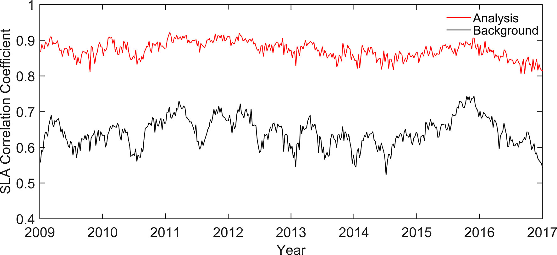
Figure 1 Daily spatial correction coefficient of SLA between analysis (red) [background (black)] field and altimeter observation within 50°S–50°N.

The high-resolution multi-scale assimilation process is as follows. First, the daily altimeter SLA is converted into synthetic T–S profiles, and the daily-averaged background fields of temperature and salinity are adjusted by using the multi-grid 3D-Var to assimilate those profiles and satellite SST. Second, the multi-grid 3D-Var and FGAT algorithms are used to assimilate in-situ temperature profiles to adjust the instantaneous background temperature field, and the T–S relationship constraint is used to complete the adjustment of the instantaneous background salinity field. Finally, the final adjustment of the instantaneous background salinity field is completed by assimilating in-situ salinity profiles using the multi-grid 3D-Var and FGAT algorithms. In-situ T–S profiles (above 2,000 m) and daily satellite SST are assimilated every day with a 1-day time window. The altimeter-derived T–S profiles above 1,000 m within 50°S–50°N are assimilated every 7 days with a 1-day time window.

Compared with CORA1, an advantage of CORA2 is that it can provide tidal information. To improve tidal accuracy, we employed the nudging method proposed by Fu et al. (2021) to restore the surface tidal elevation of the forecast model toward that of TPXO8 at each integration time. Fu et al. (2021) suggested that this method can not only improve the accuracy of surface tidal elevation but also optimize the subsurface temperature and salinity disruptions caused by tides. Here, we show the amplitude and phase of M₂ and K₁ tidal constituents obtained by using harmonic analysis for the sea-surface height field of CORA2 and the simulation (Figure 2). The comparison between CORA2 and the simulation reveals that tidal assimilation can significantly improve the accuracy of tidal signals. It should be noted that the assimilation of daily altimeter SLA was performed to adjust meso-scale eddies, and the assimilation of surface tidal elevation was performed to improve tidal information accuracy.

FIGURE 2

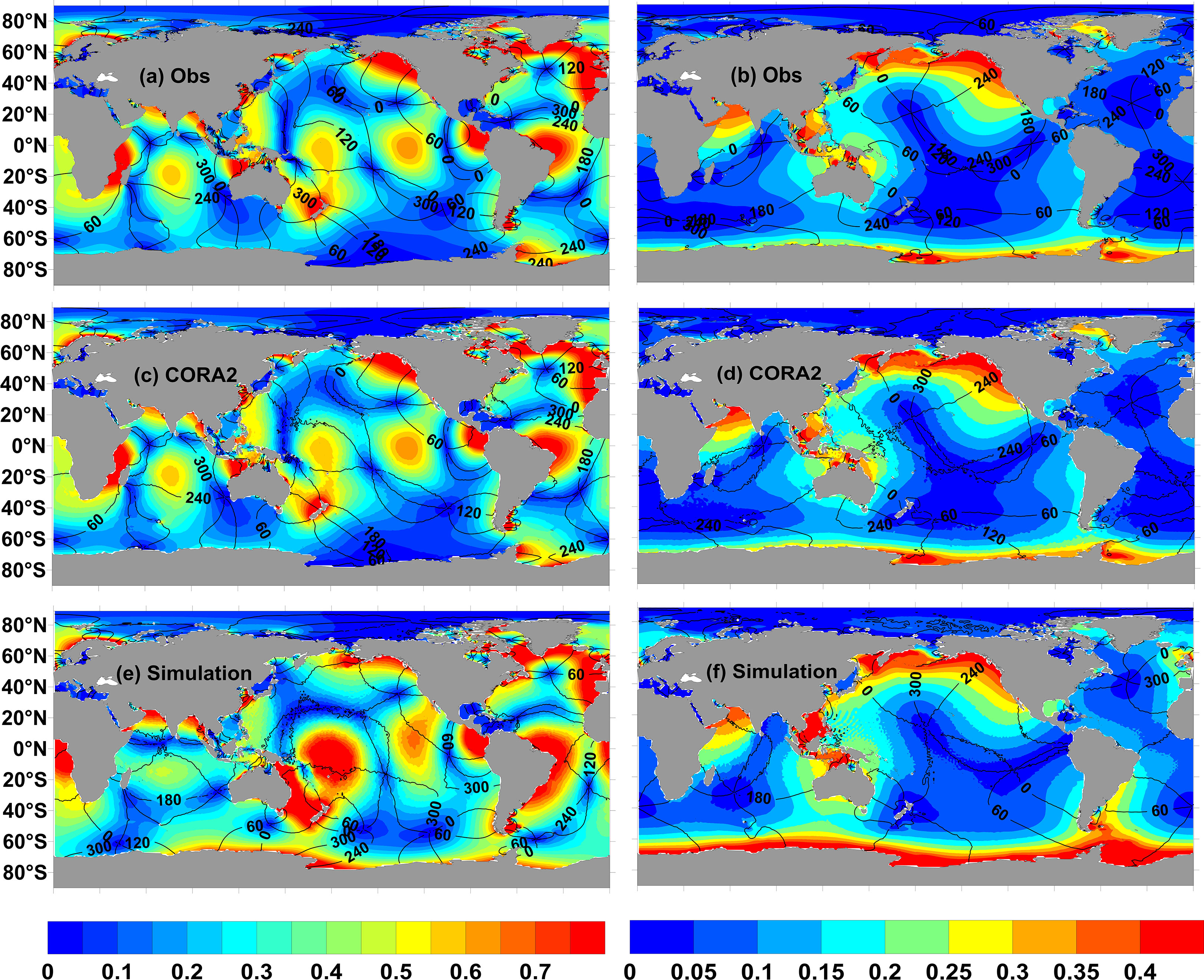
Figure 2 M2 (A, C, E) and K1 (B, D, F) amplitude (shading; units: m) and phase (contour; units: °) of surface tidal elevation in TPXO8 (A, B); a barotropic tide model constrained by observation data), China Ocean ReAnalysis version 2 (CORA2) (C, D; with tidal assimilation), and the simulation results (E, F; without tidal assimilation).

2.4 Surface forcing and spin-up

The atmospheric forcing variables include wind at a 10-m height, air temperature and humidity at a 2-m height, total precipitation, and surface downward shortwave and longwave radiative fluxes, which are taken from the Japanese Meteorological Agency reanalyses JRA-25, spanning from 1980 to 2013, and JRA-55, spanning from 2014 to 2019 (Onogi et al., 2007; Kobayashi et al., 2015). The bulk formulae of Large and Pond (1981; 1982) are used to calculate surface fluxes for the open oceans. Surface fluxes over sea ice are calculated based on the method in Parkinson and Washington (1979). Monthly climatology of river runoff is applied along the land mask and treated as freshwater flux (Fekete et al., 2002).

The generation of initial conditions for CORA2 includes the following phases. First, the numerical model is freely integrated for 10 model years starting from the temperature and salinity fields from WOA18, with the climatological atmospheric forcing. This is followed by a 6-year simulation period, driven by the 1980–1985 JRA-25 atmospheric forcing. Then, in-situ T–S profiles and satellite SST are assimilated to adjust the model to observations since 1986. Altimeter observation is assimilated from 1997. After that, when the system was integrated until 2009, it is found that there is a slightly large error, with a temperature root-mean-square error (RMSE) of >1.3°C and salinity RMSE of >0.25 psu in the Atlantic Ocean. The error is mainly caused by the following factors: (1) the rationality test of the data range in the in-situ profile quality control procedure has a small bug for the Atlantic Ocean; (2) there is an excessive reuse of the high-density in-situ profiles; and (3) owing to the overflow of high-salinity water from the Mediterranean Sea in the deep layer, the T–S relationship is relatively complex in the North Atlantic Ocean, and the simple temperature-to-salinity mapping adjustment algorithm proposed by Troccoli et al. (2002) is not applicable. The assimilation scheme is optimized to address the above problems, including through the fine tuning of the in-situ profile quality control procedure, the thinning of high-density in-situ profiles, and the limiting of the T–S relationship constraint range, for the integration from 2009 onward.

The ocean variables in the CORA2 product, including sea surface height (SSH), 3D temperature, salinity, and current, are saved on a uniform horizontal grid of 0.1° × 0.1° and 50 layers at 3-hour intervals. The tide signals are embodied in the oceanic variables. The derived daily and monthly datasets spanning from 1989 to 2019 are calculated and released on the websites http://mds.nmdis.org.cn and http://www.cmoc-china.cn. In this study, we focus only on the reanalysis products during the Argo-rich period, namely 2004–2019.

3 Other analysis and reanalysis datasets

The reanalysis products GLORYS12v1 (Lellouche et al., 2021), HYCOM (GLBu0.08; Cummings and Smedstad, 2013), GREP (version 2; Storto et al., 2019a), ECCO4 (version 4r4; Forget et al., 2015), and SODA3 (version 3.4.2; Carton et al., 2018) are used here for inter-comparison, and their characteristics are given in Table S1 in the Supplementary Material.

GLORYS12v1 is a global eddy-resolving ocean reanalysis spanning 1993 to 2020 with a horizontal resolution of 0.083°. The surface atmospheric fields are from the European Centre for Medium Range Weather Forecasts (ECMWF) ERA-Interim reanalysis. Reprocessed along-track altimeter SLA from the CMEMS, the Advanced Very High Resolution Radiometer (AVHRR) SST from the NOAA, SIC from the Centre d’Exploitation et de Recherche SATellitaire (CERSAT), and in-situ T–S profiles from the CMEMS are jointly assimilated using a Singular Extended Evolutive Kalman (SEEK) filter with a 7-day assimilation cycle. GLORYS12v1 uses the incremental analysis update (IAU) procedure in Bloom et al. (1996) to weaken shocks and spurious waves introduced by the “classical” model correction, where analysis increments would be applied in a one-time step.

The outputs from HYCOM experiment GLBu0.08 versions 19.1 and 19.0, covering the period from October 1992 to December 2012, are used in this study. The horizontal resolution is 0.083°. Surface forcing is from the National Centers for Environmental Prediction (NCEP) Climate Forecast System Reanalysis (CFSR) with a horizontal resolution of 0.3° and temporal resolution of 1 hour. The time window for observation assimilation is 1 day. Along-track satellite SST data are assimilated to maintain a diurnal cycle in the model. The Modular Ocean Data Assimilation System (MODAS) is used to project along-track altimeter SLA to depth in the form of synthetic T–S profiles. The final analysis increments are inserted into the model over a 6-hour time period using the IAU procedure.

Version 2 of GREP is a four-member ensemble reanalysis with a horizontal resolution of 0.25° and 75 standard z-levels spanning 1993 to 2020. All ensemble members use the NEMO (Nucleus for European Modelling of the Ocean) ocean model, which is forced by the ECMWF ERA-Interim atmospheric forcing, albeit with different bulk formulae and employing different observational datasets and data assimilation schemes. A preliminary assessment of GREP indicates that the ensemble mean outperforms all individual members in approaching in-situ profiles (Storto et al., 2019a).

Version 4 of the ECCO uses the MITgcm to reconstruct ocean and sea-ice states from 1992 to 2017, with a horizontal resolution of 0.5°. ECCO4 employs a 4D-Var method to modify initial conditions, parameters, and surface forcing fields to minimize analysis-minus-observation misfits in a least-squares sense. Assimilated observation data include SLA from the satellite altimeter, SST from satellite radiometers (AVHRR), sea surface salinity (SSS) from the Aquarius satellite radiometer/scatterometer, ocean bottom pressure (OBP) from the Gravity Recovery and Climate Experiment (GRACE) satellite gravimeter, SIC from satellite radiometers (Special sensor microwave/imager and Special Sensor Microwave Imager Sounder), and in-situ T–S profiles from the the World Ocean Circulation Experiment (WOCE), the Global Ocean Ship-based Hydrographic Investigations Program (GO-SHIP), Argo, and so on.

SODA3 (version 3.4.2) reconstructs ocean and sea-ice states from 1980 to 2017. Its horizontal resolution is 0.25°. The surface forcing is from the ECMWF ERA-Interim reanalysis. SODA3 assimilates WOD T–S profiles, International Comprehensive Ocean-Atmosphere Data Set (ICOADS) in-situ observation, and satellite SST (the NOAA Advanced Clear-Sky Processor for Ocean Level 2P SST product) using an optimal interpolation scheme. The IAU procedure is implemented using an update cycle of 10 days.

Objective analysis EN4 ENACT/ENSEMBLES version4 (version 4.2.1) of subsurface temperature and salinity from the Met Office Hadley Centre (Good et al., 2013) is used in the study. It provides gridded data of 1° × 1° × 42 levels and is a monthly complete-spatial-coverage objective analysis. The latest satellite OSTIA SST data with a horizontal resolution of 1/20° (Good et al., 2020) are also used to calculate the RMSE, bias, and correlation coefficient of the SSTs of reanalysis products.

4 Comparison of CORA2 with CORA1

The main differences and improvements of CORA2 with respect to its previous version, CORA1, are described here. We analyze both versions to understand which improvements in the CORA2 system are due to system changes. First, SST RMSEs and biases with respect to the OISST SST in CORA2 are compared with those in CORA1 (Figures 3A, B). The difference in SST biases between CORA2 and CORA1 is not very large, except for a bias excursion in 2013 for CORA1. However, the SST RMSE of CORA2 is significantly smaller than that of CORA1. In CORA1, the satellite OISST SST data were assimilated by using a surface relaxation scheme, and its constraint effect was decided by the relaxation coefficient. In CORA2, the OISST SST is assimilated using the multi-grid 3D-Var method with a 1-day assimilation cycle. The error relative to non-independent observations is mainly decided by the assimilation scheme. Therefore, we suggest that the current satellite SST assimilation scheme in CORA2 is more advantageous for constraining the SST to the observation. Of course, there may also be other factors that cause the reduction of CORA2 SST error, such as the atmospheric forcing change and the resolution improvement.

FIGURE 3

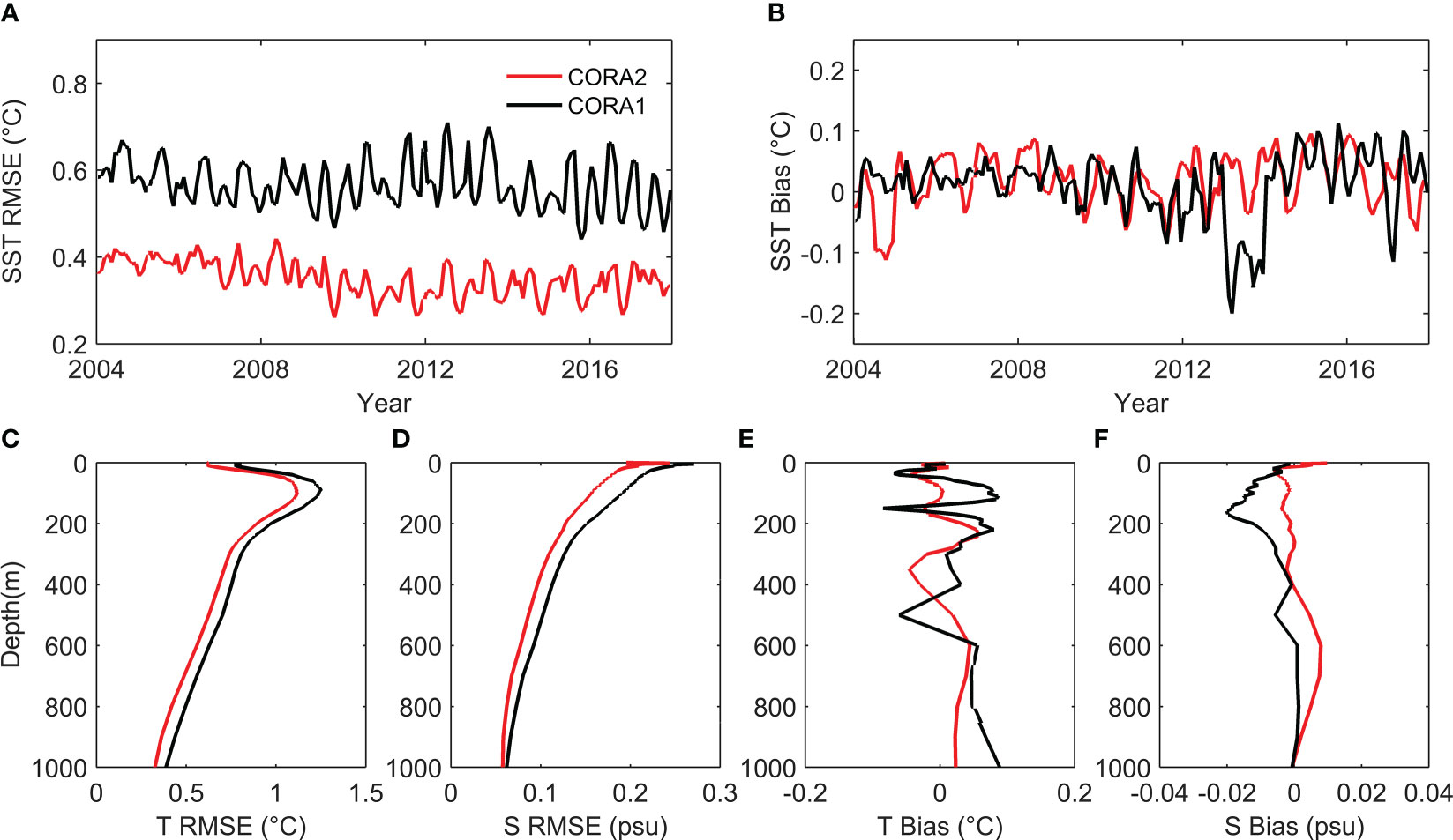
Figure 3 Time series of root-mean-square errors (RMSEs) (A; units: °C) and biases (B; reanalysis minus observation; units: °C) of monthly SST for CORA2 (red) and CORA1 (black) with respect to OISST sea-surface temperature (SST) within 70°S–70°N. Vertical distributions (0–1,000 m) of RMSEs (C, D) and biases (E, F) of monthly temperature (C, E; units: °C) and salinity (D, F; units: psu) for China Ocean ReAnalysis version 2 (CORA2) (red) and China Ocean ReAnalysis version 1 (CORA1) (black) with respect to Argo profiles in the global oceans during the period of 2004–2017.

Figure 3 also shows that the RMSEs and biases in subsurface temperature and salinity with respect to the Argo profiles in CORA2 are smaller than those in CORA1. For the assimilation of in-situ T–S profiles, CORA2 and CORA1 use the same basic assimilation method, namely multi-grid 3D-Var; however, compared with CORA1, CORA2 has improved resolution and used the FGAT method to achieve high-resolution assimilation. CORA2 also adds tidal forcing and assimilation to resolve some small-scale internal tidal signals contained in the in-situ T–S profiles. These changes may be the main reasons for the improvement in subsurface temperature and salinity accuracy in CORA2.

Compared with CORA1, a significant improvement of CORA2 is the enhancement of the spatial resolution from the eddy-permitting to the eddy-resolving level. To evaluate its ability to reproduce meso-scale eddy signals, the temporal and spatial distributions of eddy kinetic energy (EKE) are calculated based on daily velocity. Figure 4A shows the temporal evolution of the monthly three-dimensional means of EKE over 0–300 m during the period 2010–2017. CORA2 shows higher EKE than CORA1. Figure 4B demonstrates that all the large dynamic systems are well represented by CORA2, including the western boundary currents, Agulhas recirculation, and Antarctic Circumpolar Current (ACC). The EKE level in CORA2 is of the same order of magnitude as that of GLORYS12v1, with a similar resolution (Lellouche et al., 2021). A comparison of CORA2 and CORA1 shows an obvious increase in EKE alongside the increased resolution (Figure 4C).

FIGURE 4

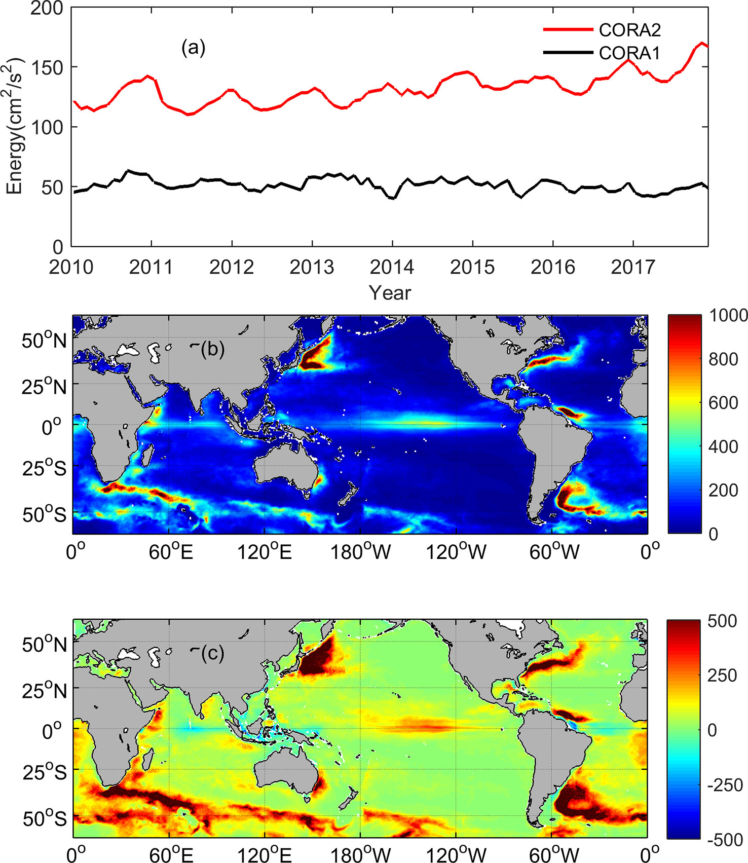
Figure 4 (A) Three-dimensional mean of monthly eddy kinetic energy (EKE) (cm²/s²) at 0–300 m depth for the China Ocean ReAnalysis version 2(CORA2) (red) and China Ocean ReAnalysis version 1 (CORA1) (black). (B) Average EKE (cm²/s²) at 0-300 m depth during 2010–2017 for CORA2 and (C) the differences when compared with CORA1 (CORA2 minus CORA1).

5 Comparison of CORA2 with other reanalyses

We first compare the RMSEs, biases, and correlation coefficients of monthly SSTs for the six reanalysis products (CORA2, GLORYS12v1, HYCOM, GREP, SODA3, and ECCO4). For subsurface temperature and salinity evaluation, we project the monthly reanalyzed 3D temperature and salinity onto in-situ profile locations to obtain analysis-minus-observation misfits. We then analyze the time and space errors (RMSE and bias) statistically. The in-situ profiles are divided into two groups: the assimilated Argo data and the non-assimilated in-situ profiles. The gridded SLA assimilated in CORA2 is also used to evaluate the fidelity of temporal variability in various ocean reanalyses. Considering the different time periods covered by the various products, we evaluate monthly SST, 3D temperature and salinity, and SLA over 2004–2017 for all reanalyses, except for HYCOM (2004–2012). In addition, through comparison with the objective analysis EN4, we also assess variations in monthly steric sea level (including thermosteric and halosteric components) and ocean heat content (OHC) in CORA2, GLORYS12v1, and GREP using the time period of 2004–2019.

5.1 SST

We compare the temperature at the shallowest reanalysis level to the OSTIA SST. Figure 5A shows that the SST RMSE of GREP is the smallest and that of ECCO4 is the largest of the six reanalyses, and that the SST RMSE of CORA2 becomes closer to that of GREP from 2009 onward. SODA3 has a slightly smaller SST RMSE than ECCO4 and a larger SST RMSE than HYCOM and GLORYS12v1. The high accuracy of GREP may be attributed to its ensemble nature (Masina et al., 2017). The daily assimilation of gridded SST in CORA2 greatly constrains the modeled SST to closely match the observations. Although the resolutions of GLORYS12v1 and HYCOM are similar to that of CORA2, the 7-day assimilation cycle in GLORYS12v1 and the along-track SST assimilation in HYCOM provide a relatively weak SST constraint. For SODA3, because the 10-day assimilation cycle is relatively long, the analyzed SST RMSE is relatively large. The largest SST departure of ECCO4 may be related to its assimilation scheme, which tends to maintain the conservation of ocean energy and mass rather than place a mandatory constraint on SST. Compared with the RMSEs, the spread of biases in the six reanalyses is small (Figure 5B). Each reanalysis has a spatial correlation coefficient above 0.99, which means that they can effectively reproduce the spatial structures of SST (Figure 5C).

FIGURE 5

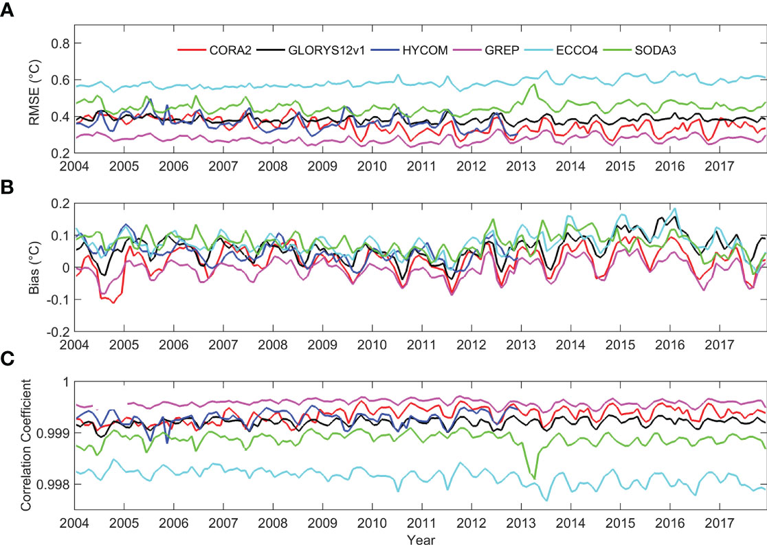
Figure 5 Time series of (A) root-mean-square errors (RMSEs) (units: °C), (B) biases (units: °C; reanalysis minus observation), and (C) spatial correlation coefficients of monthly sea-surface temperature (SST) relative to OSTIA SST within 70°S–70°N for CORA2 (China Ocean ReAnalysis version 2) (red), GLORYS12v1 (Global Ocean reanalysis and Simulation) (black), HYCOM (HYbrid Coordinate Ocean Model) (blue), GREP (Global ocean Reanalysis Ensemble Product) (pink), ECCO4 (Estimating the Circulation and Climate of the Ocean, version 4) (cyan), and SODA3 (Simple Ocean Data Assimilation, version 3) (green).

The spatial patterns of SST RMSE of the six products are similar. Low error mainly occurs in the open seas and high error in coastal waters, western boundary currents, and ACC area (Figure 6). The large errors in the coastal waters, western boundary currents, and ACC area may be associated with the poor representation of strong non-linear dynamic processes and the displacement of SST fronts. Similar to results in the time series of RMSE, the SST RMSEs of CORA2 and GREP are the lowest, being less than 0.3°C in the ocean interior and greater than 0.6°C in the western boundary currents and ACC area. The SST error of ECCO4 is the largest, being less than 0.5°C in the ocean interior and greater than 0.8°C in the western boundary currents and ACC area extending to the coastal waters. The error levels of GLORYS12v1, HYCOM, and SODA3 lie between those of ECCO4 and CORA2/GREP. We also note that the SST RMSE of CORA2 is greater than that of the other products in the Okhotsk Sea, which may be related to the freezing and melting of sea ice. The ratios of the standard deviation of reanalysis SSTs relative to that of the OSTIA SST were also estimated to analyze SST variability (Figure S1 in the Supplementary Material).

FIGURE 6

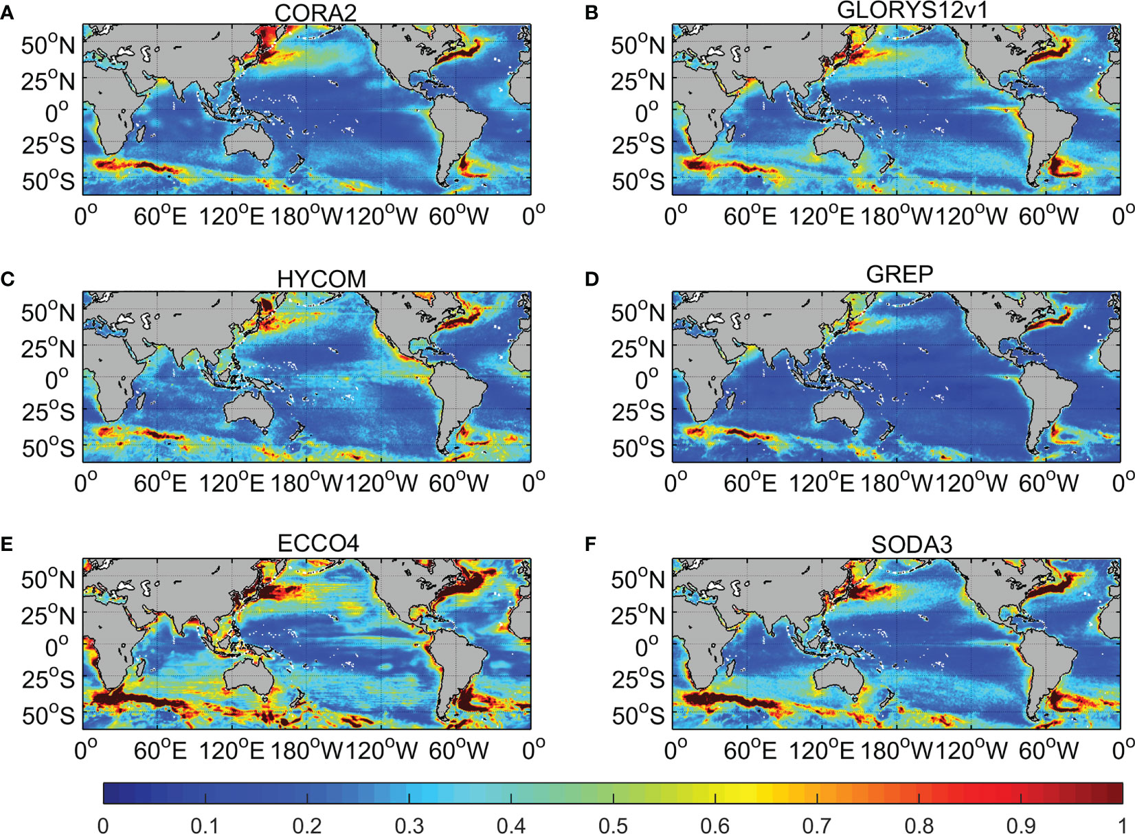
Figure 6 Spatial distributions of the root-mean-square error (RMSE) (units: °C) of monthly sea-surface temperature (SST) with respect to OSTIA SST for CORA2 (China Ocean ReAnalysis version 2) (A), GLORYS12v1 (Global Ocean reanalysis and Simulation) (B), HYCOM (HYbrid Coordinate Ocean Model) (C), GREP (Global ocean Reanalysis Ensemble Product) (D), ECCO4 (Estimating the Circulation and Climate of the Ocean, version 4) (E), and SODA3 (Simple Ocean Data Assimilation, version 3) (F). All RMSEs are computed for the period 2004–2017, except for HYCOM (2004–2012).

5.2 Subsurface temperature and salinity

In this subsection, we use Argo profiles to assess the subsurface performance of CORA2 relative to the other reanalyses. Considering that the use of monthly means does not compromise the skill score statistics during an observation-rich period (Storto et al., 2019a), we focus on the monthly mean fields of temperature and salinity. The vertical distributions of the temperature and salinity RMSEs and biases of the six reanalyses are shown in Figure 7. For all reanalyses, the highest temperature RMSE occurs near the thermocline. The temperature RMSE of CORA2 is similar to that of SODA3, lower than that of ECCO4, and larger than those of GLORYS12v1, GREP, and HYCOM. Owing to the uncertainties in the surface freshwater flux and runoff, the highest salinity RMSE occurs near the sea surface. GREP and GLORYS12v1 have the smallest salinity RMSEs and ECCO4 and SODA3 have the largest salinity RMSEs. Compared with the other products, the salinity RMSE of CORA2 is at a medium level. The large salinity RMSE of SODA3 might be related to the large salinity error in the Mediterranean Sea region (Figure S2 in the Supplementary Document).

FIGURE 7

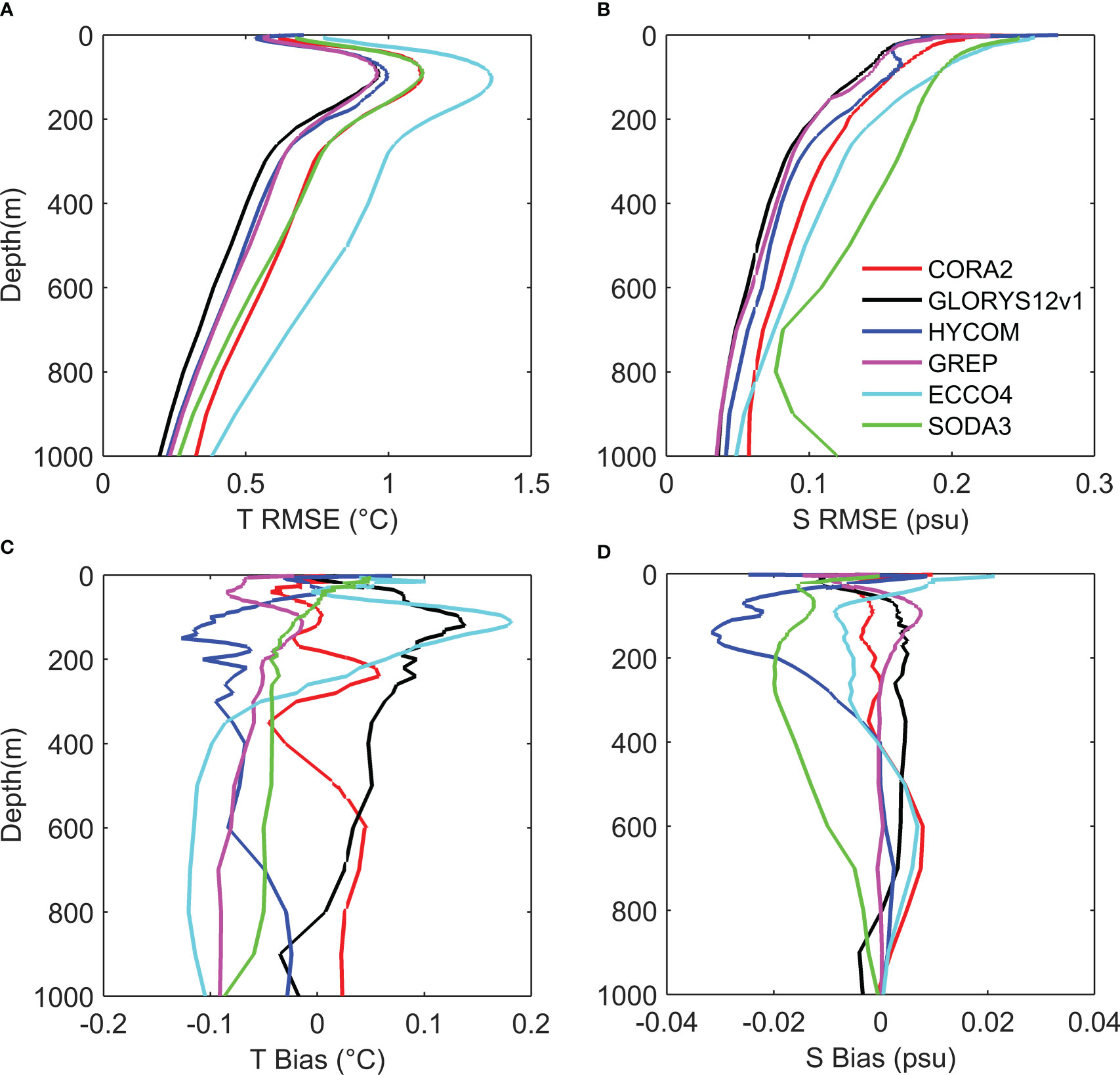
Figure 7 Vertical distributions (0–1,000 m) of root-mean-square errors (RMSEs) (A, B) and biases (reanalysis minus observation; C, D) of monthly temperature (A, C; units: °C) and salinity (B, D; units: psu) for the six reanalyses [CORA2 (China Ocean ReAnalysis version 2), red; GLORYS12v1 (Global Ocean reanalysis and Simulation), black; HYCOM (HYbrid Coordinate Ocean Model), blue; GREP (Global ocean Reanalysis Ensemble Product), pink; ECCO4 (Estimating the Circulation and Climate of the Ocean, version 4), cyan; SODA3 (Simple Ocean Data Assimilation, version 3), green] with respect to Argo profiles in the global oceans. RMSE and bias are computed between 2004 and 2017 for all reanalyses, except for HYCOM (2004–2012).

In the upper ocean, although the temperature bias of CORA2 shows an obvious positive and negative alternation structure, its average is near zero (Figure 7C). The positive and negative alternation may be caused by the misplacement of thermocline depth. Compared with CORA2, the temperatures of GREP, HYCOM, and SODA3 show significant negative biases, while those of GLORYS12v1 and ECCO4 show significant positive biases. For salinity, the biases are relatively small for all the products except SODA3 and HYCOM.

Spatial distributions of RMSEs of the monthly temperature of the six reanalyses averaged over 0–2,000 m are displayed in Figure 8. Temperature RMSEs show similar spatial structures in all six reanalyses. The large errors in strong current areas, for example, the Gulf Stream, Kuroshio, and equatorial currents, may be caused by the misplacement of fronts, eddies, and thermocline. Table 1 shows the RMSEs for the six reanalyses in 12 areas. In the ocean interior, i.e., the North Indian Ocean, South Indian Ocean, Northeast Pacific, South Pacific, South Atlantic, and Southern Ocean, GLORYS12v1, HYCOM, and GREP have errors of between 0.44°C and 0.76°C, while CORA2 and SODA3 have slightly larger errors, of between 0.48°C and 0.82°C. ECCO4 has the largest errors, of between 0.61°C and 1.05°C. In the areas of the Gulf Stream, Kuroshio, and equatorial currents, the RMSEs of GLORYS12v1, HYCOM, and GREP increase to 0.79–0.98°C, those of CORA2 and SODA3 increase to 0.90–1.27°C, and the RMSE of ECCO4 increases to 1.06–1.52°C. ECCO4 has the largest RMSE, reaching 1.07°C in the global oceans, while CORA2 and SODA3 have medium RMSEs of 0.87°C. HYCOM, GREP, and GLORYS12v1 have the smallest RMSEs, of 0.73–0.75°C, in the global oceans.

FIGURE 8

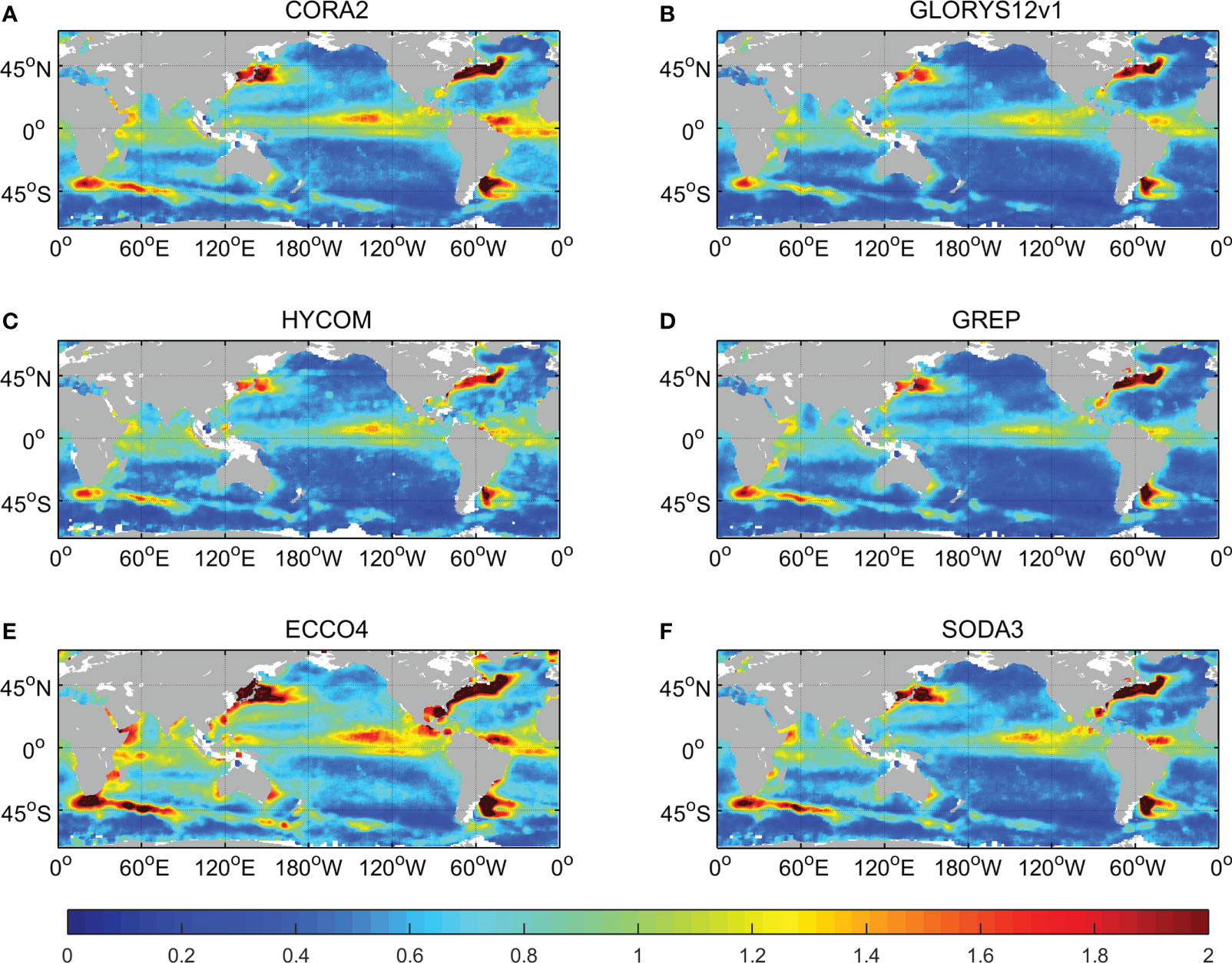
Figure 8 Spatial distributions of monthly temperature root-mean-square error (RMSE) (units: °C) of the six reanalyses [CORA2 (China Ocean ReAnalysis version 2), (A); GLORYS12v1 (Global Ocean reanalysis and Simulation), (B); HYCOM (HYbrid Coordinate Ocean Model), (C); GREP (Global ocean Reanalysis Ensemble Product), (D); ECCO4 (Estimating the Circulation and Climate of the Ocean, version 4), (E); SODA3 (Simple Ocean Data Assimilation, version 3), (F)] with respect to Argo profiles over 0–2,000 m. RMSE is computed between 2004 and 2017 for all reanalyses, except for HYCOM (2004–2012).

TABLE 1

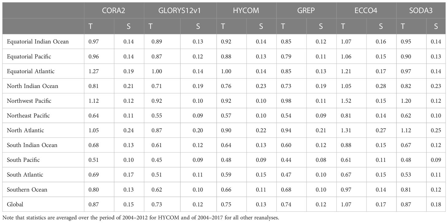
Table 1 Root-mean-square errors (RMSEs) of monthly reanalyses [CORA2 (China Ocean ReAnalysis version 2), GLORYS12v1 (Global Ocean reanalysis and Simulation), HYCOM (HYbrid Coordinate Ocean Model), GREP (Global ocean Reanalysis Ensemble Product), ECCO4 (Estimating the Circulation and Climate of the Ocean, version 4), SODA3 (Simple Ocean Data Assimilation, version 3)] temperature (T; units: °C) and salinity (S; units: psu) against Argo profiles in the equatorial Indian Ocean (40–100°E, 10°S–10°N), equatorial Pacific (130°E–80°W, 10°S–10°N), equatorial Atlantic (50°W–0°, 10°S–10°N), North Indian Ocean (40–100°E, 10–30°N), Northwest Pacific (120–180°E, 12–50°N), Northeast Pacific (180°E–90°W, 12–50°N), North Atlantic (80°W–0°, 12–50°N), South Indian Ocean (40–120°E, 30–10°S), South Pacific (150°E–80°W, 30–10°S), South Atlantic (50°W–0°, 30–10°S), Southern Ocean (180°E–180°W, 60–30°S), and global oceans.

Figure 9 is the same as Figure 8, but for salinity. The spatial patterns of salinity RMSE are similar for the six reanalyses, with small errors occurring in the ocean interior and large errors in coastal areas. The large RMSEs are generally associated with the uncertainties of climatological runoff and freshwater flux. Table 1 shows that the salinity RMSE of CORA2 (0.15 psu) in the global oceans is larger than the salinity RMSEs of GLORYS12v1 (0.12 psu), GREP (0.12 psu), and HYCOM (0.13 psu), but smaller than those of ECCO4 (0.17 psu) and SODA3 (0.18 psu). Large RMSEs, of more than 0.20 psu, are found mainly in the North Indian Ocean and Atlantic Ocean for the six reanalyses. In addition, the large salinity RMSE of SODA3 in the Mediterranean Sea is consistent with the result mentioned above (Figure S2 in the Supplementary Document).

FIGURE 9

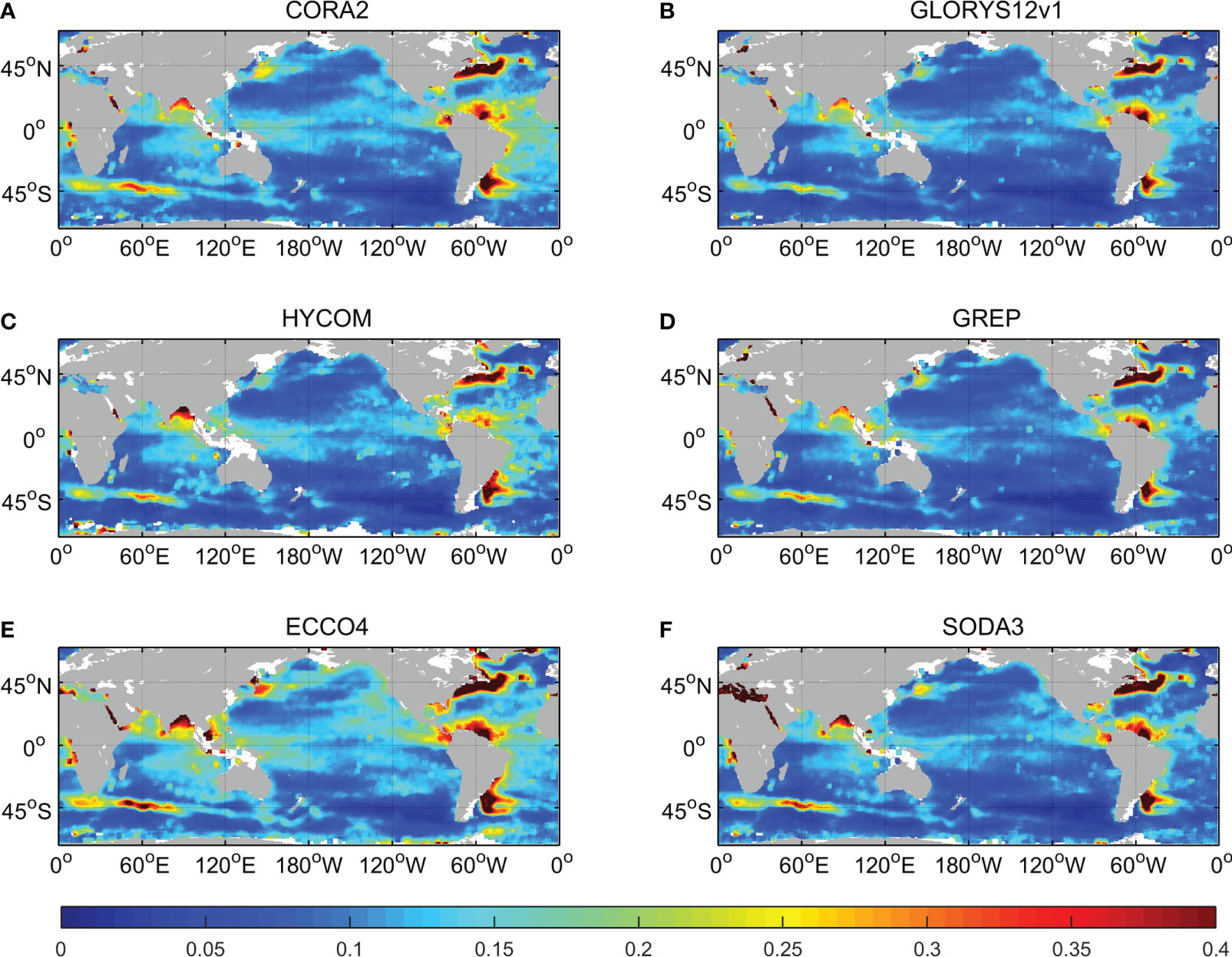
Figure 9 Spatial distributions of monthly salinity root-mean-square error (RMSE) (units: psu) of the six reanalyses [CORA2 (China Ocean ReAnalysis version 2), (A); GLORYS12v1 (Global Ocean reanalysis and Simulation), (B); HYCOM (HYbrid Coordinate Ocean Model), (C); GREP (Global ocean Reanalysis Ensemble Product), (D); ECCO4 (Estimating the Circulation and Climate of the Ocean, version 4), (E) SODA3 (Simple Ocean Data Assimilation, version 3), (F)] with respect to Argo profiles over 0–2,000 m. RMSE is computed between 2004 and 2017 for all reanalyses, except for HYCOM (2004–2012).

Similar to Table 1, Table S2 in the Supplementary Material gives the biases of temperature and salinity for the six reanalyses in the 12 ocean areas. The temperature (salinity) biases in the global oceans are –0.003°C (–0.002 psu), 0.058°C (0.000 psu), –0.052°C (–0.014 psu), –0.060°C (0.001 psu), 0.033°C (–0.001 psu), and –0.024°C (–0.012 psu) for CORA2, GLORYS12v1, HYOM, GREP, ECCO4, and SODA3, respectively. Generally, the absolute value of the bias in the Atlantic Ocean is larger than the absolute bias values in the other regions for all the reanalysis products.

Figure 10 shows the RMSE time series of various reanalyses in the Indian, Pacific, Atlantic, and global oceans. We can see that the temperature RMSEs of all products decrease with time, which may be due to the increasing number of assimilated observations. The accuracy of CORA2 is similar to that of SODA3 in the Pacific, Indian, and Atlantic oceans during 2009–2017. We find that the RMSE in the Atlantic for CORA2 is relatively large before 2009 and sharply declines after we optimized the quality control procedure and assimilation scheme of temperature and salinity for the year 2009 onward. In addition, the salinity error of SODA3 in the global ocean increases rapidly after 2011, which may be caused by the large salinity error in the Mediterranean region.

FIGURE 10

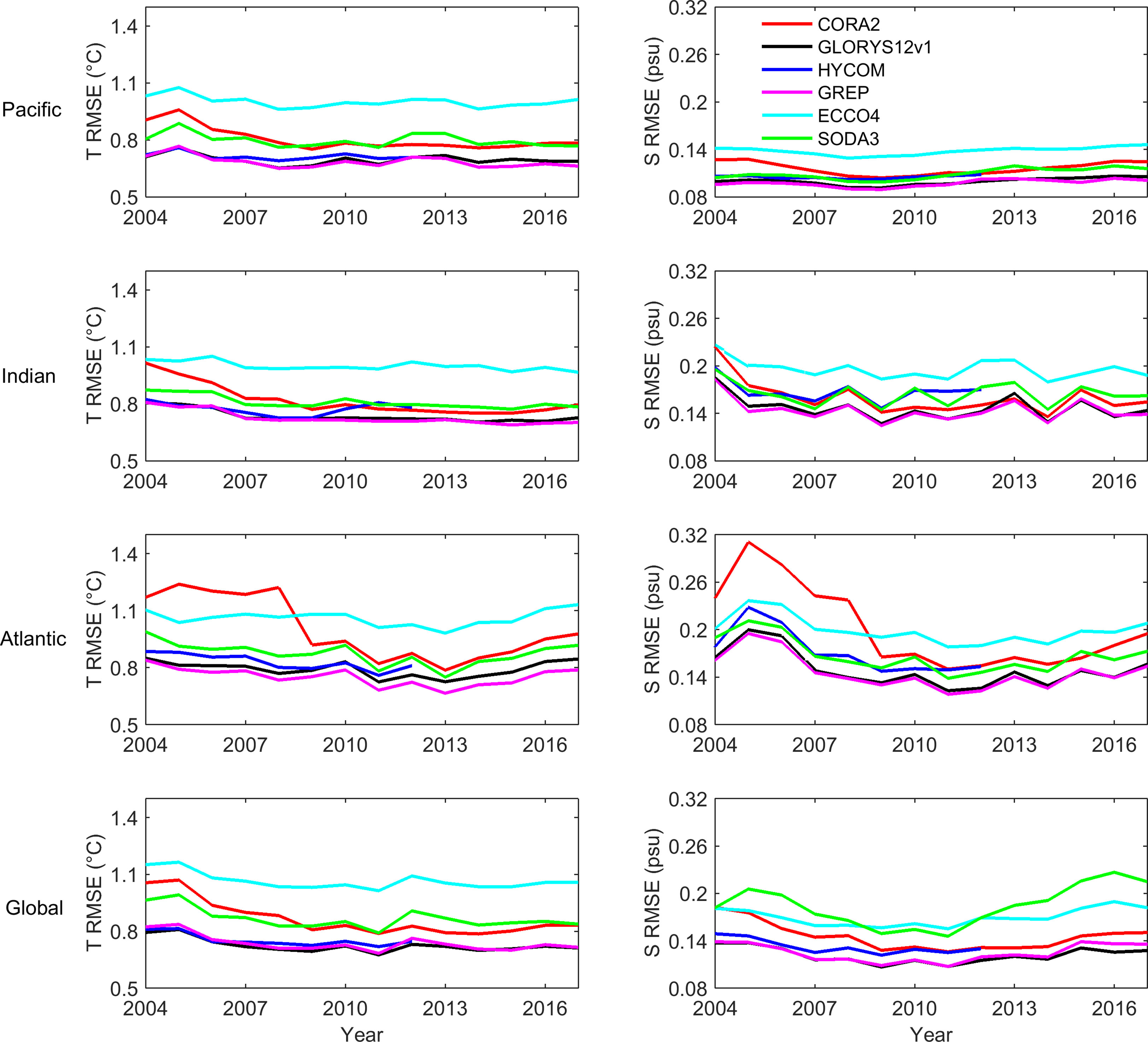
Figure 10 Time series of root-mean-square error (RMSE) of the six reanalyses [CORA2 (China Ocean ReAnalysis version 2), red; GLORYS12v1 (Global Ocean reanalysis and Simulation), black; HYCOM (HYbrid Coordinate Ocean Model), blue; GREP (Global ocean Reanalysis Ensemble Product), pink; ECCO4 (Estimating the Circulation and Climate of the Ocean, version 4), cyan; SODA3 (Simple Ocean Data Assimilation, version 3), green] with respect to Argo profiles for temperature (left panels; units: °C) and salinity (right panels; units: psu) over 0–2,000 m in the Pacific, Indian, Atlantic, and global oceans.

We chose independent observations from a station at 117.5°E, 19.0°N to further validate the performance of the reanalyses, which comprises the cross-shaped observational array of buoys and moorings in the northern South China Sea deployed by China (Zhang et al., 2016). To better compare the variability at the sub-monthly scale, we analyzed daily reanalysis products, i.e., CORA2, GLORYS12v1, GREP, and ECCO4. Figure 11 plots the time series of temperature (Figure 11, left panels) and salinity (Figure 11, right panels) profiles at the station from 1 August 2014 to 28 February 2015 for the observations and for the four reanalyses. The observations exhibit an obvious seasonal variability, with the deepening (August–December 2014) and shoaling (January–February 2015) of the thermocline and halocline, and some sub-monthly-scale disruptions, such as the sinking (day 100) and rising (day 125) of the water column. The four reanalyses can all describe the seasonal variabilities. Owing to their higher resolution, GLORYS12v1 and CORA2 can better depict sub-monthly-scale variability than GREP and ECCO4. GLORYS12v1 has the smallest temperature and salinity RMSEs of 0.78°C and 0.14 psu, respectively. Because of the smoother, warmer, and saltier characteristics of ECCO4, it has the largest RMSEs, exhibiting the worst skill score. Compared with the observations, there are several shocks and spurious waves in the temperature and salinity fields of CORA2; these may be caused by the use of tidal forcing and the assimilation scheme, which simply adds the analysis increment in one step rather than gradually absorbing it.

FIGURE 11

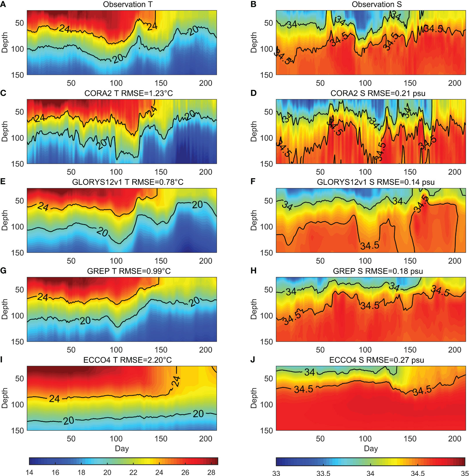
Figure 11 Time series of daily temperature (left; units: °C) and salinity (right; units: psu) profiles at a station (117.5°E, 19.0°N) from 1 August 2014 to 28 February 2015 for observations (A, B), CORA2 (China Ocean ReAnalysis version 2) (C, D), GLORYS12v1 (Global Ocean reanalysis and Simulation) (E, F), GREP (Global ocean Reanalysis Ensemble Product) (G, H), and ECCO4 (Estimating the Circulation and Climate of the Ocean, version 4) (I, J). Root-mean-square errors (RMSEs) of temperature and salinity for the four reanalyses are also given.

5.3 Sea level

Monthly sea-level fields in the different reanalysis products were compared with that of the gridded AVISO absolute dynamic topography (ADT) to evaluate their ability to reproduce sea-level variability. CORA2 and HYCOM assimilate the T–S profiles derived by altimeter SLA, while GLORYS12v1 and ECCO4 assimilate along-track altimeter SLA. Thus, the gridded AVISO ADT is not directly assimilated in these reanalyses. Figure 12 shows the spatial distribution of the temporal correlation coefficients of monthly sea level between the reanalyses and satellite observations. GLORYS12v1 and GREP have the highest correlation coefficients, exceeding 0.8 in most regions. HYCOM is comparable to GLORYS12v1 and GREP in the Pacific and Indian oceans, but not in the Atlantic Ocean. CORA2 has higher correlation coefficients in the Pacific Ocean and Indian Ocean and a lower correlation coefficient in the Atlantic Ocean than ECCO4 and SODA3. Considering that the assimilation scheme of SLA used in CORA2 relies on background fields, the large temperature and salinity errors in the Atlantic are probably responsible for the low correlation coefficients. The lowest correlation for SODA3 is mainly due to the absence of sea-level assimilation.

FIGURE 12

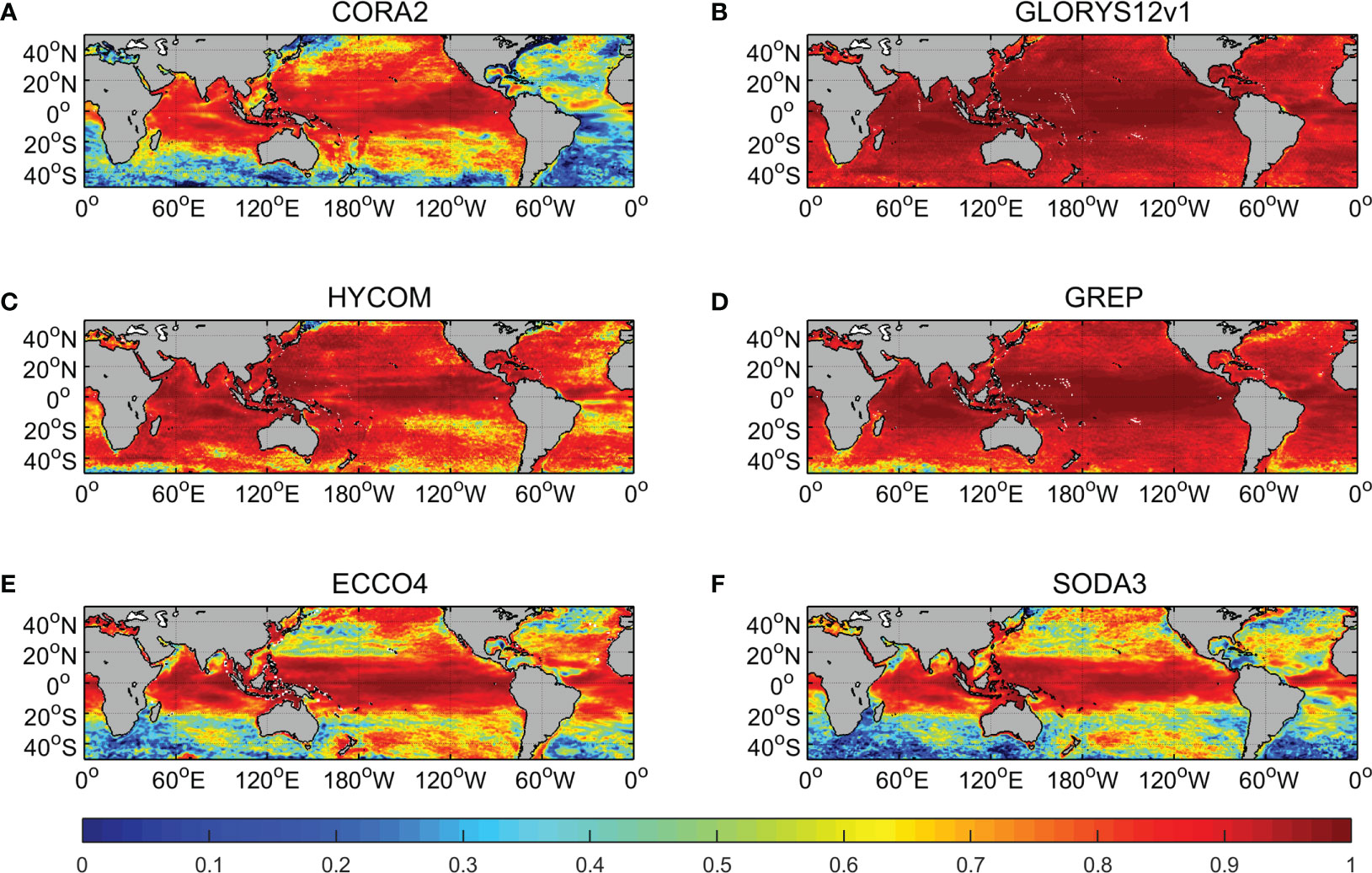
Figure 12 Spatial distributions of the temporal correlation coefficient between reanalyses [CORA2 (China Ocean ReAnalysis version 2) (A), GLORYS12v1 (Global Ocean reanalysis and Simulation) (B), HYCOM (HYbrid Coordinate Ocean Model) (C), GREP (Global ocean Reanalysis Ensemble Product) (D), ECCO4 (Estimating the Circulation and Climate of the Ocean, version 4) (E), and SODA3 (Simple Ocean Data Assimilation, version 3) (F)] and AVISO altimeter data from Copernicus Marine Environment Monitoring (CMEMS). Statistics are computed using monthly mean sea level during 2004–2017 for all reanalyses, except for HYCOM (2004–2012).

5.4 Steric sea level

Global mean sea level (GMSL) can be decomposed into steric change and mass change, while the steric change can in turn be decomposed into thermosteric and halosteric changes. In this subsection, we compare globally averaged values of steric sea level and its thermosteric and halosteric components in CORA2 with those in the high-resolution reanalysis GLORYS12v1, the ensemble reanalysis GREP, and the objective analysis EN4. The calculation algorithm for steric, thermosteric, and halosteric sea levels is similar to that of Storto et al. (2017), and the global average includes the upper 1,000-m layer between 60°S and 60°N. Figure 13 shows that the four products satisfactorily capture the global steric sea-level seasonality, while they show large discrepancies in inter-annual variabilities and trends. The time series of CORA2 and GLORYS12v1, which have eddying-resolving resolutions, show more complex structures than those of EN4 and GREP, which have only eddying-permitting resolutions. The steric sea-level trends of EN4, CORA2, GLORYS12v1, and GREP during the period 2009–2019 are 0.80, 1.16, 1.48, and 1.05 mm/year, respectively. Storto et al. (2017) estimated a global steric sea-level trend at full depth during 1993–2010 based on the reanalysis ensemble mean, with the value of 1.02 ± 0.05 mm/year. Compared with Storto et al. (2017), our vertical integration depth is shallower and the time period is more recent, but the total linear trend of the ensemble reanalysis GREP is still very close to their results. The linear trend of CORA2 is closer to that of GREP relative to the other products, meaning a good skill score in terms of reproducing steric sea-level change. The trend of the objective analysis EN4 is smaller than that of ensemble reanalysis GREP; Storto et al. (2017) also suggested that its predecessor EN3 has a smaller linear trend relative to the reanalysis ensemble mean. For the four products, the thermosteric component dominates the change in steric sea-level trend, which is consistent with previous estimates (Storto et al., 2017; Zuo et al., 2017), and their trends range from 1.01 to 1.71 mm/year. The halosteric components exhibit negative trends for the four products, ranging from –0.22 to –0.03 mm/year. The thermosteric and halosteric component trends of CORA2 and GREP are also the closest among the four products.

FIGURE 13

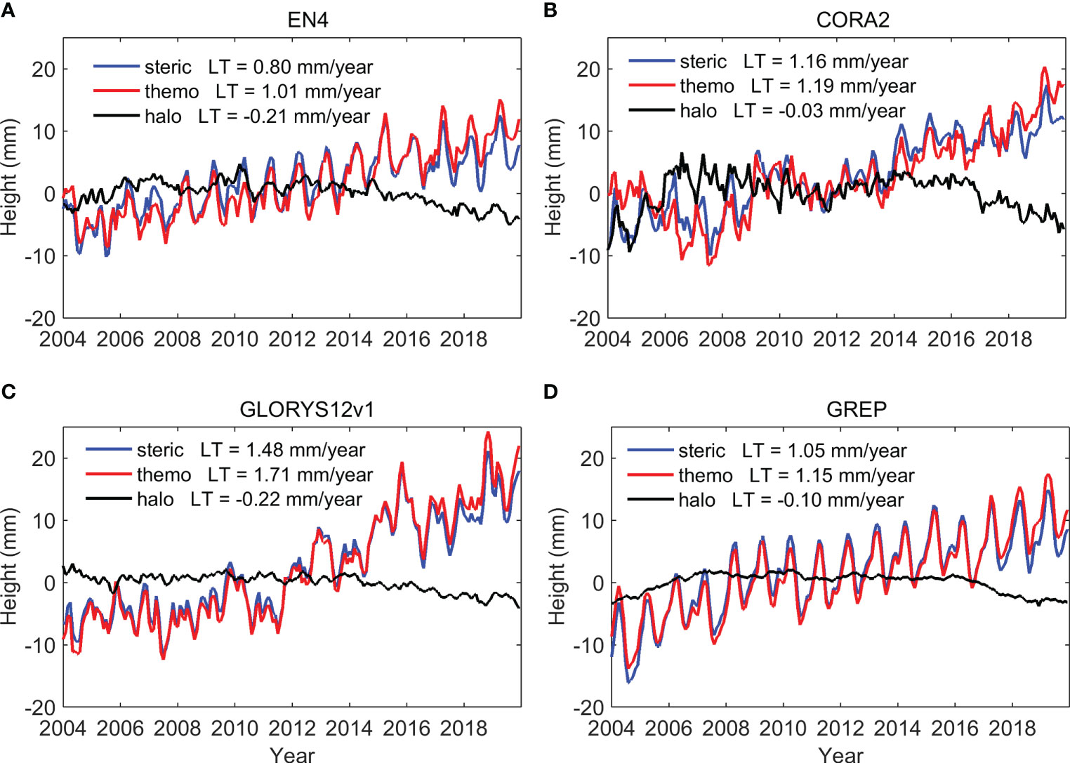
Figure 13 Monthly time series of global steric (blue), thermosteric (red), and halosteric (black) sea level (units: mm) for EN4, (A) CORA2 (China Ocean ReAnalysis version 2) (B), GLORYS12v1 (Global Ocean reanalysis and Simulation) (C), and GREP (Global ocean Reanalysis Ensemble Product) (D) during the period of 2004–2019. LT: linear trend during 2009–2019.

5.5 Ocean heat content

To assess the capability of the products to describe climate variability, we selected four key areas that are related to the climate indexes for the Indian Ocean Dipole (IOD), El Niño–Southern Oscillation (ENSO), Pacific Decadal Oscillation (PDO), and Atlantic Meridional Overturning Circulation (AMOC): the IOD Western (W) area (western equatorial Indian Ocean), NINO3 (Niño 3 Index) area, Northeast (NE) Pacific, and North (N) Atlantic. Yearly ocean heat content (OHC) anomalies in different regions over 0–300, 0–700, and 0–1,500 m depth ranges were calculated from EN4, CORA2, GLORYS12v1, and GREP (Figure 14).

FIGURE 14

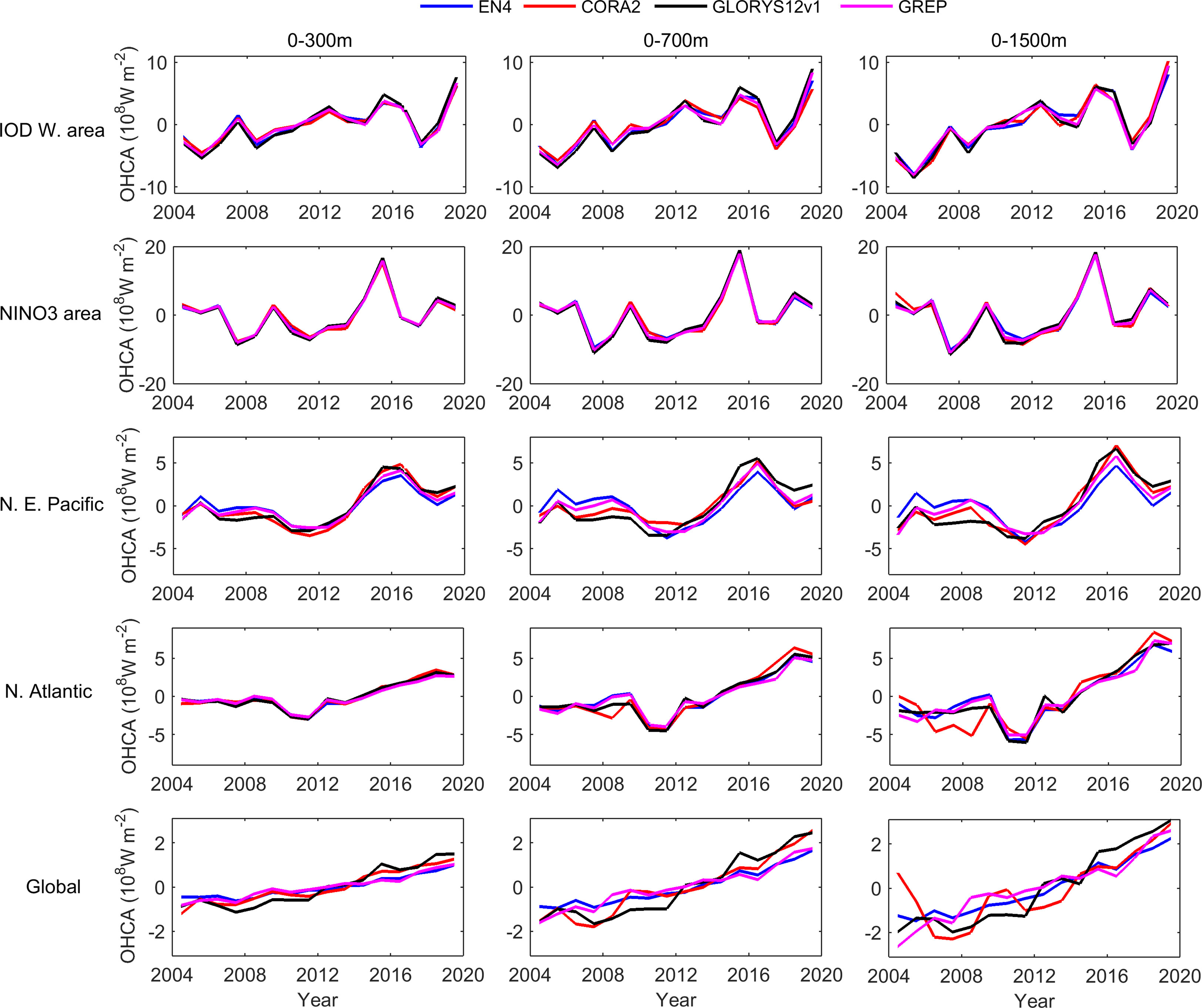
Figure 14 Time series of ocean heat content (OHC anomalies (10⁸ W m^–2) in the Indian Ocean Dipole (IOD) West area (50–70°E, 10°S–10°N), NINO3 area (150–90°W, 5°S–5°N), Northeast Pacific (160–120°W, 20–50°N), North Atlantic (80°W–0°, 20–50°N), and global oceans for EN4 (blue), CORA2 (China Ocean ReAnalysis version 2) (red), GLORYS12v1 (Global Ocean reanalysis and Simulation) (black), and GREP (Global ocean Reanalysis Ensemble Product) (pink) at depths of 0–300 m (left panels), 0–700 m (middle panels), and 0–1,500 m (right panels). OHC anomaly is expressed as the equivalent heating rate in W m^–2, relative to the region’s ocean surface area.

Figure 14 shows that the four products present similar OHC time series at 0–300 m, including a prominent inter-annual variability in the IOD W and NINO3 areas, an inter-decadal variability in the NE Pacific, and a warming trend in the N Atlantic and global oceans. Similar to previous findings (Balmaseda et al., 2015; Palmer et al., 2017; Wang et al., 2018; Storto et al., 2019a), OHC varies on different time scales. The large inter-annual variabilities in the equatorial Pacific and Indian oceans are associated with the ENSO and IOD, respectively. Three peaks of OHC anomalies in the IOD W area match the IOD warm events in 2006, 2012, and 2015, respectively. Two peaks in the NINO3 area correspond to the strong EI Niño events in 2010 and 2016, respectively. In the NE Pacific, the negative OHC anomalies during 2004–2013 coincide with the cold PDO phase and the positive OHC anomalies during 2014–2019 coincide with the warm PDO phase, which matches previous studies (Palmer et al., 2017). In the N Atlantic, the four products show similar warming trends and local small-scale disturbances. The warming trend reflects a weakening subpolar gyre and a slowdown of the deep western boundary current off Labrador, which is thought to be an indicator of the slowdown of the AMOC (Zhang, 2008; Palmer et al., 2017). The curves of the global mean OHC from the four datasets broadly overlap and represent the global warming trend in the upper ocean. We also found that the warming of the North Atlantic subpolar gyre is enhanced relative to the global oceans, supporting the results of Palmer et al. (2017).

The 0–700 and 0–1,500 m OHC anomalies show similar variabilities to the 0–300 m OHC anomalies. However, the four products start to diverge when vertical integration is carried out at deeper levels. Palmer et al. (2017) suggested that the large spread in the amplitude of OHC anomalies at deeper levels may be caused by the lack of observational data. There are more small-scale disturbances in the rising trends of global OHC anomalies for CORA2 and GLORYS12v1 than for EN4 and GREP. Similar results were presented by Storto et al. (2019a), who showed that a regional product with high resolution can exhibit finer-scale structures than a global ensemble mean. The abnormity of the global 0–1,500 m OHC anomalies of CORA2 around 2004 should be treated with caution, and the possible cause requires further analysis. In the N Atlantic, the large deviation of the 0–1,500 m OHC anomalies of CORA2 from the other products before 2009 is consistent with the large RMSEs of temperature and salinity discussed in Section 5.2.

For the global OHC in the upper 1,500 m, the long-term trends over 2004–2019 vary from 0.97 (GREP), 1.03 (EN4), 1.31 (CORA2), to 1.54 × 10²³ J/decade (GLORYS12v1); most of them are larger than the results of Wang et al. (2018) based on objective analyses during 1998–2012, which vary from 0.81 to 1.0 × 10²³ J/decade. In addition, the trends of the products with a high resolution (CORA2 and GLORYS12v1) are larger than those with a low resolution (EN4 and GREP).

6 Summary and discussion

We described the China Ocean ReAnalysis version 2 (CORA2), presenting an inter-comparison with its predecessor CORA1 and other popular reanalysis products in terms of observed variables and some climate variabilities. CORA2 is based on the eddy-resolving MITgcm, including interactive sea ice in the high latitudes and tidal forcing. The in-situ T–S profiles, daily gridded satellite SLA and SST are assimilated by a high-resolution multi-scale data assimilation method. The surface tidal elevation from TPXO8 is assimilated by the nudging method. The daily satellite SLA can adjust meso-scale eddies, while the TPXO8 data can improve the accuracy of surface and subsurface tidal signals (Fu et al., 2021). The improvement of CORA2 relative to CORA1 and how CORA2 compares with other selected products is presented by analyzing reanalysis misfits to independent and non-independent observations and by comparing the variability of EKE, steric sea level, and OHC. The evaluation results show the advantages and disadvantages of the ocean reanalysis CORA2.

Compared with CORA1, the surface and subsurface T–S errors of CORA2 with respect to non-independent observations are significantly reduced owing to the enhanced resolution, the updated SST assimilation scheme, the use of an FGAT assimilation scheme, and the inclusion of tidal forcing and assimilation. The EKE of CORA2 sharply increases compared with that of CORA1 and is consistent with that of GLORYS12v1, demonstrating that high-resolution reanalyses have a higher EKE than low-resolution ones.

The comparison between the six reanalyses and OSTIA SST reveals that the SST accuracy of CORA2 is more similar to that of GREP and with a smaller error than the other reanalyses since 2009. It is speculated that the high accuracy of CORA2 largely stems from the 1-day assimilation cycle of SST.

Compared with the non-independent Argo profiles, the T–S RMSE of CORA2 is similar to that of SODA3, lower than that of ECCO4, and higher than those of GLORYS12v1 and GREP in most oceans. Although the T–S RMSE of CORA2 is slightly larger in the Atlantic Ocean, it was reduced after we fixed the bug. The CORA2 bias is close to zero, while the other products have some biases, especially for the temperature field. For the variability of subsurface T–S, ECCO4 exhibits a poor performance while GREP shows good seasonal variation; GLORYS12v1 and CORA2 can not only describe the seasonal features but also some sub-monthly-scale fluctuations, owing to their high resolutions. There are several shocks and spurious waves in the time evolution of CORA2, which may be caused by adding the analysis increment to the background state in a single time step and/or including tidal signals. The large RMSE of ECCO4 may be attributed to the fact that its assimilation method of 4D-Var tends to maintain dynamic consistency.

The SLA of CORA2 is significantly correlated with the altimetry in the Indian and Pacific oceans, but the correlation in the Atlantic is weak. This may be associated with the fact that the SLA assimilation method depends on the background temperature and salinity fields, and their errors in the Atlantic are larger than those in the other two regions. The poor performance of SODA3 is attributed to the absence of altimeter SLA constraints. The seasonal variability of global steric sea level and the proportion of thermosteric and halosteric components can be well described in all the products, while the time series of high-resolution products (CORA2 and GLORYS12v1) show more complex structures than those of low-resolution products (EN4 and GREP). The linear trend of global steric sea level of CORA2 is closer to that of ensemble reanalysis GREP, smaller than that of GLORYS12v1, and larger than that of EN4.

The time series of global OHC anomalies of EN4, CORA2, GLORYS12v1, and GREP show the best agreement, representing the climate variability related to the IOD, ENSO, PDO, and AMOC indices, as well as the global warming trend. The accuracy of the products in representing climate variability gradually decreases with increased depth, owing to the lack of observation constraints. In the Atlantic, the large T–S errors of CORA2 cause the 0–1,500 m OHC to deviate from the average value over 2004–2008, but do not change the overall variation characteristics. The long-term trends of global OHC in the high-resolution reanalyses (CORA2 and GLORYS12v1) are larger than those in the low-resolution reanalyses (EN4 and GREP) and they are also larger than the result of Wang et al. (2018).

It should be noted that a good reanalysis product should use a fixed ocean model and data assimilation scheme with the best available parameterizations, observations, and meteorological forcing, which do not change during the production. However, it is not possible to rerun the entire CORA2 reanalysis according to best practices owing to computational cost, leading to some changes in the CORA2 system during the long integration process: for example, the optimization of the assimilation scheme in 2009 and the change of atmospheric forcing data in 2014. In particular, the optimization of the assimilation scheme has brought obvious improvements to the accuracy of CORA2 in the Atlantic Ocean since 2009.

CORA2 is a complex system, resulting from extensive efforts to combine information and developments from observations, assimilation, and modeling communities. Given the strengths and weaknesses of CORA2 discussed in this paper, key improvements to CORA2 in the future should include the assimilation of the best available observation data (e.g., satellite OSTIA SST, SSS, and sea ice concentration data), the use of the IAU procedure, the improvement of the SLA assimilation method. At the same time, it is necessary to further assess the sea ice, currents, and tides of CORA2 to meet the needs of users in different fields.

Data availability statement

The raw data supporting the conclusions of this article will be made available by the authors, without undue reservation.

Author contributions

HF integrated the CORA2 reanalysis system, made the products, participated in the validation and inter-comparison, and wrote the original manuscript. BD optimized the reanalysis system and standardized the outputs of the reanalysis products. ZG processed the tide gauge observations and participated in the validation. XW was in charge of the reanalysis system, debugged the assimilation code, performed the assimilation experiments, and modified the manuscript. GC processed the in-situ T–S profiles. LZ participated in the parameterization of the numerical model. YZ participated in the inter-comparison and validation. KL engaged in tide analysis and assimilation. XZ focused on the validation. WL designed the assimilation scheme and coded the original assimilation code. All authors contributed to the article and approved the submitted version.

Acknowledgments

The authors thank the three reviewers GR, SM and PW for their careful reading and for providing very constructive comments that improved the paper. This research was jointly supported by the National Key R&D Program of China (2019YFC1510002, 2021YFC3101603 and 2016YFC1401800) and National Natural Science Foundation of China (41976019).

Conflict of interest

The authors declare that the research was conducted in the absence of any commercial or financial relationships that could be construed as a potential conflict of interest.

Publisher’s note

All claims expressed in this article are solely those of the authors and do not necessarily represent those of their affiliated organizations, or those of the publisher, the editors and the reviewers. Any product that may be evaluated in this article, or claim that may be made by its manufacturer, is not guaranteed or endorsed by the publisher.

Supplementary material

The Supplementary Material for this article can be found online at: https://www.frontiersin.org/articles/10.3389/fmars.2023.1084186/full#supplementary-material

Supplementary Table 1 | List of five ocean reanalyses used in this study and their main characteristics.

Supplementary Table 2 | Biases of monthly reanalyses [CORA2 (China Ocean ReAnalysis version 2), GLORYS12v1 (Global Ocean reanalysis and Simulation), HYCOM (HYbrid Coordinate Ocean Model), GREP (Global ocean Reanalysis Ensemble Product), ECCO4 (Estimating the Circulation and Climate of the Ocean, version 4), SODA3 (Simple Ocean Data Assimilation, version 3)] temperature (T; units: °C) and salinity (S; units: psu) against Argo profiles in the equatorial Indian Ocean (40–100°E, 10°S–10°N), equatorial Pacific (130°E–80°W, 10°S–10°N), equatorial Atlantic (50°W–0°, 10°S–10°N), North Indian Ocean (40–100°E, 10–30°N), Northwest Pacific (120–180°E, 12–50°N), Northeast Pacific (180°E–90°W, 12–50°N), North Atlantic (80°W–0°, 12–50°N), South Indian Ocean (40–120°E, 30–10°S), South Pacific (150°E–80°W, 3–10°S), South Atlantic (50°W–0°, 30–10°S), Southern Ocean (180°E–180°W, 60–30°S), and global oceans Note that statistics are averaged over the period 2004–2012 for HYCOM and the period 2004–2017 for other reanalyses.

Supplementary Figure 1 | Ratios of standard deviation of monthly sea-surface temperature (SST) of CORA2 (China Ocean ReAnalysis version 2) (A), GLORYS12v1 (Global Ocean reanalysis and Simulation) (B), HYCOM (HYbrid Coordinate Ocean Model) (C), GREP (Global ocean Reanalysis Ensemble Product) (D), ECCO4 (Estimating the Circulation and Climate of the Ocean, version 4) (E), and SODA3 (Simple Ocean Data Assimilation, version 3) (F) relative to that of OSTIA SST during 2004–2017 (2004–2012 for HYCOM). The SST variances of CORA2 and GREP are the closest to the observation, and the ratios remain around one in most regions. The SST variance of GLORYS12v1 in the Antarctic Circumpolar Current (ACC) region is larger than the observation, and the ratio can reach >1.2. The HYCOM result is the most different from those of the other products, which may be related to its short time period.

Supplementary Figure 2 | Vertical distribution of root-mean-square errors (RMSEs) (A) and biases (B) of monthly salinity (units: psu) of SODA3 with respect to Argo profiles in the global oceans, including (red) and excluding (black) the Mediterranean Sea.

References

Adcroft A., Campin J. (2004). Rescaled height coordinates for accurate representation of free-surface flows in ocean circulation models. Ocean Model. 7, 269–284. doi: 10.1016/j.ocemod.2003.09.003

CrossRef Full Text | Google Scholar

Arbic B., Garner S., Hallberg R., Simmons H. (2004). The accuracy of surface elevations in forward global barotropic and baroclinic tide models. Deep-Sea Res. II. 51, 3069–3101. doi: 10.1016/j.dsr2.2004.09.014

CrossRef Full Text | Google Scholar

Balmaseda M., Hernandez F., Storto A., Palmer M., Alves O., Shi L., et al. (2015). The ocean reanalyses intercomparison project (ORA-IP). J. Oper. Oceanogr. 8 (sup1), s80–s97. doi: 10.1080/1755876X.2015.1022329

CrossRef Full Text | Google Scholar

Balmaseda M., Mogensen K., Weaver A. (2012). Evaluation of the ECMWF ocean reanalysis system ORAS4. Q. J. R. Meteorol. Soc. 139, 1132–1161. doi: 10.1002/qj.2063

CrossRef Full Text | Google Scholar

Blockley E., Martin M., McLaren A., Ryan A., Waters J., Lea D., et al. (2014). Recent development of the met office operational ocean forecasting system: an overview and assessment of the new global FOAM forecasts. Geosci. Model. Dev. 7 (6), 2613–2638. doi: 10.5194/gmd-7-2613-2014

CrossRef Full Text | Google Scholar

Bloom S., Takacs L., Da Silva A., Ledvina D. (1996). Data assimilation using incremental analysis updates. Mon. Weather Rev. 124, 1256–1271. doi: 10.1175/1520-0493(1996)124<1256:DAUIAU>2.0.CO;2

CrossRef Full Text | Google Scholar

Carton J., Chepurin G., Chen L. (2018). SODA3: a new ocean climate reanalysis. J. Climate. 31 (17), 6967–6983. doi: 10.1175/JCLI-D-18-0149.1

CrossRef Full Text | Google Scholar

Carton J., Stephen G., Kalnay E. (2019). Temperature and salinity variability in the SODA3, ECCO4r3, and ORAS5 ocean reanalyses 1993-2015. J. Climate. 32, 2277–2293. doi: 10.1175/JCLI-D-18-0605.1

CrossRef Full Text | Google Scholar

Chevallier M., Smith G., Dupont F., Lemieux J., Forget G., Fujii Y., et al. (2017). Intercomparison of the Arctic sea ice cover in global ocean–sea ice reanalyses from the ORA-IP project. Clim. Dyn. 49, 1107–1136. doi: 10.1007/s00382-016-2985-y

CrossRef Full Text | Google Scholar

Cooper M., Haines K. (1996). Altimetric assimilation with water property conservation. J. Geophys. Res. 24, 1059–1077. doi: 10.1029/95JC02902

CrossRef Full Text | Google Scholar

Cummings J., Smedstad O. (2013). Variational data assimilation for the global ocean. data assimilation for atmospheric. Oceanic Hydrologic Appl. 2 (13), 303–343. doi: 10.1007/978-3-642-35088-7_13

CrossRef Full Text | Google Scholar

Egbert G. D., Erofeeva S. Y. (2002). Efficient inverse modeling of barotropic ocean tides. J. Atmos. Ocean Tech. 19, 183–204. doi: 10.1175/1520-0426(2002)019<0183:EIMOBO>2.0.CO;2

CrossRef Full Text | Google Scholar

Fekete B., Vörösmarty C., Grabs W. (2002). High-resolution fields of global runoff combining observed river discharge and simulated water balances. Global Biogeochem. Cy. 16, 15.1–15.10. doi: 10.1029/1999GB001254

CrossRef Full Text | Google Scholar

Forget G., Campin J., Heimbach P., Hill C., Ponte R., Wunsch C. (2015). ECCO version 4: an integrated framework for non-linear inverse modeling and global ocean state estimation. Geosci. Model. Dev. 8 (10), 3071–3104. doi: 10.5194/gmd-8-3071-2015

CrossRef Full Text | Google Scholar

Fu H., Wu X., Li W., Zhang L., Liu K., Dan B. (2021). Improving the accuracy of barotropic and internal tides embedded in a high-resolution global ocean circulation model of MITgcm. Ocean Model. 162, 101809. doi: 10.1016/j.ocemod.2021.101809

CrossRef Full Text | Google Scholar

Garcia H., Boyer T., Locarnini R., Baranova O., Zweng M. (2018). World ocean database 2018: user’s manual (prerelease). Ed. Mishonov A. (Silver Spring, MD: NOAA). Available at: https://www.NCEI.noaa.gov/OC5/WOD/pr_wod.html.

Google Scholar

Good S., Fiedler E., Mao C., Martin M. J., Maycock A., Reid R., et al. (2020). The current configuration of the OSTIA system for operational production of foundation Sea surface temperature and ice concentration analyses. Remote Sens. 12, 720. doi: 10.3390/rs12040720

CrossRef Full Text | Google Scholar

Good S., Martin M., Rayner N. (2013). EN4: quality controlled ocean temperature and salinity profiles and monthly objective analyses with uncertainty estimates. J. Geophys. Res. 118, 6704–6716. doi: 10.1002/2013JC009067

CrossRef Full Text | Google Scholar

Griffies S., Hallberg R. (2000). Bibarmonic friction with a smagorinsky-like viscosity for use in Large-scale eddy-permitting ocean models. Monthly Weather Rev. 128, 2935–2946. doi: 10.1175/1520-0493(2000)128<2935:BFWASL>2.0.CO;2

CrossRef Full Text | Google Scholar

Han G., Fu H., Zhang X., Li W., Wu X., Wang X., et al. (2013b). A global ocean reanalysis products in the China ocean reanalysis (CORA) project. Adv. Atmos. Sci. 30 (6), 1621–1631. doi: 10.1007/s00376-013-2198-9

CrossRef Full Text | Google Scholar

Han G., Li W., Zhang X., Li D., He Z., Wang X., et al. (2011). A regional ocean reanalysis system for coastal waters of China and adjacent seas. Adv. Atmos. Sci. 28 (3), 682–690. doi: 10.1007/s00376-010-9184-2

CrossRef Full Text | Google Scholar

Han G., Li W., Zhang X., Wang X., Wu X., Fu H., et al. (2013a). A new version of regional ocean reanalysis for coastal waters of China and adjacent seas. Adv. Atmos. Sci. 30 (4), 974–982. doi: 10.1007/s00376-012-2195-4

CrossRef Full Text | Google Scholar

Karspeck A., Stammer D., Köhl A., Danabasoglu G., Balmaseda M., Smith D., et al. (2017). Comparison of the Atlantic meridional overturning circulation between 1960 and 2007 in six ocean reanalysis products. Clim. Dyn. 49, 957–982. doi: 10.1007/s00382-015-2787-7

CrossRef Full Text | Google Scholar

Kobayashi S., Ota Y., Harada Y., Ebita A., Moriya M., Onoda H., et al. (2015). The JRA-55 reanalysis: general specifications and basic characteristics. J. Meteor. Soc. Japan. 93, 5–48. doi: 10.2151/jmsj.2015-001

CrossRef Full Text | Google Scholar

Large W., McWilliams J., Doney S. (1994). Oceanic vertical mixing: a review and a model with a nonlocal boundary layer parameterization. Rev. Geophys. 32, 363–403. doi: 10.1029/94RG01872

CrossRef Full Text | Google Scholar

Large W., Pond S. (1981). Open ocean momentum flux measurements in moderate to strong winds. J. Phys. Oceanogr. 11 (3), 324–336. doi: 10.1175/1520-0485(1981)011<0324:OOMFMI>2.0.CO;2

CrossRef Full Text | Google Scholar

Large W., Pond S. (1982). Sensible and latent heat flux measurements over the ocean. J. Phys. Oceanogr. 12 (5), 464–482. doi: 10.1175/1520-0485(1982)012<0464:SALHFM>2.0.CO;2

CrossRef Full Text | Google Scholar

Lellouche J., Greiner E., Bourdalle-Badié R., Garric G., Melet A., Drévillon M., et al. (2021). The Copernicus global 1/12° oceanic and Sea ice GLORYS12 reanalysis. Front. Earth Sci. 9. doi: 10.3389/feart.2021.698876

CrossRef Full Text | Google Scholar

Li W., Xie Y., He Z., Han G., Liu K., Ma J., et al. (2008). Application of the multi-grid data assimilation scheme to the China seas' temper-ature forecast. J. Atmos. Oceanic Technol. 25 (11), 2106–2116. doi: 10.1175/2008JTECHO510.1

CrossRef Full Text | Google Scholar

Marshall J., Adcroft A., Hill C., Perelman L., Heisey C. (1997). A finite volume, incompressible navier–stokes model for studies of the ocean on parallel computers. J. Geophys. Res. 102, 5753–5766. doi: 10.1029/96JC02775

CrossRef Full Text | Google Scholar

Masina S., Storto A. (2017). Reconstructing the recent past ocean variability: status and perspective. J. Mar. Res. 75, 727–764. doi: 10.1357/002224017823523973

CrossRef Full Text | Google Scholar

Masina S., Storto A., Ferry N., Valdivieso M., Haines K., Balmaseda M., et al. (2017). An ensemble of eddy-permitting global ocean reanalyses from the MyOcean project. Clim. Dyn. 49, 813–841. doi: 10.1007/s00382-015-2728-5

CrossRef Full Text | Google Scholar

Merchant C. J., Embury O., Bulgin C. E., Block T., Corlett G., Fiedler E., et al. (2019). Satellite-based time-series of sea-surface temperature since 1981 for climate applications. Sci. Data. 6 (223), 2052–4463. doi: 10.1038/s41597-019-0236-x

CrossRef Full Text | Google Scholar

Onogi K., Tsutsui J., Koide H., Sakamoto M., Kobayashi S., Hatsushika H., et al. (2007). The JRA-25 reanalysis. J. Met. Soc. Jap. 85 (3), 369–432. doi: 10.2151/jmsj.85.369

CrossRef Full Text | Google Scholar

Palmer M., Roberts C., Balmaseda M., Chang Y., Chepurin G., Ferry N., et al. (2017). Ocean heat content variability and change in an ensemble of ocean reanalyses. Clim. Dyn. 49, 909–930. doi: 10.1007/s00382-015-2801-0

CrossRef Full Text | Google Scholar

Parkinson C., Washington W. (1979). A large-scale numerical model of sea ice. J. Geophys. Res. 84, 311–337. doi: 10.1029/JC084iC01p00311

CrossRef Full Text | Google Scholar

Pujol M., Faugère Y., Taburet G., Dupuy S., Pelloquin C., Ablain M., et al. (2016). DUACS DT2014: the new multi-mission altimeter data set reprocessed over 20 years. Ocean Sci. 12, 1067–1090. doi: 10.5194/os-12-1067-2016

CrossRef Full Text | Google Scholar

Reynolds R., Smith T., Liu C., Chelton D., Casey K., Schlax M. (2007). Daily high-resolution-blended analyses for sea surface temperature. J. Cli. 20 (22), 5473–5496. doi: 10.1175/2007JCLI1824.1

CrossRef Full Text | Google Scholar

Storto A., Alvera-Azcárate A., Balmaseda M., Barth A., Chevallier M., Counillon F., et al. (2019b). Ocean reanalyses: recent advances and unsolved challenges. Front. Mar. Sci. 6. doi: 10.3389/fmars.2019.00418

CrossRef Full Text | Google Scholar

Storto A., Masina S., Balmaseda M., Guinehut S., Xue Y., Szekely T., et al. (2017). Steric sea level variability, (1993–2010) in an ensemble of ocean reanalyses and objective analyses. Clim. Dyn. 49, 709–729. doi: 10.1007/s00382-015-2554-9

CrossRef Full Text | Google Scholar

Storto A., Masina S., Dobricic S. (2014). Estimation and impact of nonuniform horizontal correlation length scales for global ocean physical analyses. J. Atmos. Ocean Technol. 31, 2330–2349. doi: 10.1175/JTECH-D-14-00042.1

CrossRef Full Text | Google Scholar

Storto A., Masina S., Navarra A. (2016). Evaluation of the CMCC eddy permitting global ocean physical reanalysis system (C-GLORS 1982–2012) and its assimilation components. Q. J. R. Meteorol. Soc. 142, 738–758. doi: 10.1002/qj.2673

CrossRef Full Text | Google Scholar

Storto A., Masina S., Simoncelli S., Iovino D., Cipollone A., Drevillon M., et al. (2019a). The added value of the multi-system spread information for ocean heat content and steric sea level investigations in the CMEMS GREP ensemble reanalysis product. Clim. Dyn. 53, 287–312. doi: 10.1007/s00382-018-4585-5

CrossRef Full Text | Google Scholar

Toyoda T., Fujii Y., Kuragano T., Kamachi M., Ishikawa Y., Masuda S., et al. (2017). Intercomparison and validation of the mixed layer depth fields of global ocean syntheses. Clim. Dyn. 49, 753–773. doi: 10.1007/s00382-015-2637-7

CrossRef Full Text | Google Scholar

Toyoda T., Fujii Y., Yasuda T., Usui N., Ogawa K., Kuragano T., et al. (2016). Data assimilation of sea ice concentration into a global ocean-sea ice model with corrections for atmospheric forcing and ocean temperature fields. J. Oceanogr. 72 (2), 235–262. doi: 10.1007/s10872-015-0326-0

CrossRef Full Text | Google Scholar

Troccoli A., Balmaseda M., Segschneider J., Vialard J., Anderson D., Haines K., et al. (2002). Salinity adjustments in the presence of temperature data assimilation. Mon. Wea Rev. 130, 89–102. doi: 10.1175/1520-0493(2002)130<0089:SAITPO>2.0.CO;2

CrossRef Full Text | Google Scholar

Uotila P., Goosse H., Haines K., Matthieu C., Antoine B., Clément B., et al. (2018). An assessment of ten ocean reanalyses in the polar regions. Clim. Dyn. 52, 1613–1650. doi: 10.1007/s00382-018-4242-z

CrossRef Full Text | Google Scholar

Valdivieso M., Haines K., Balmaseda M., Chang Y., Drevillon M., Ferry N., et al. (2017). An assessment of air–sea heat fluxes from ocean and coupled reanalyses. Clim. Dyn. 49, 983–1008. doi: 10.1007/s00382-015-2843-3

CrossRef Full Text | Google Scholar

Wang G., Cheng L., Abraham J., Li C. (2018). Consensuses and discrepancies of basin-scale ocean heat content changes in different ocean analyses. Clim. Dyn. 50, 2471–2487. doi: 10.1007/s00382-017-3751-5

CrossRef Full Text | Google Scholar

Zhang R. (2008). Coherent surface-subsurface fingerprint of the Atlantic meridional overturning circulation. Geophys. Res. Lett. 35, L20705. doi: 10.1029/2008GL035463

CrossRef Full Text | Google Scholar

Zhang H., Chen D., Zhou L., Liu X., Ding T., Zhou B. (2016). Upper ocean response to typhoon kalmaegi, (2014). J. Geophys. Res. Oceans. 121, 6520–6535. doi: 10.1002/2016JC012064

CrossRef Full Text | Google Scholar

Zhang J., Hibler W., Steele M., Rothrock D. (1998). Arctic Ice-ocean modeling with and without climate restoring. J. Phys. Oceanogr. 28, 191–217. doi: 10.1175/1520-0485(1998)028<0191:AIOMWA>2.0.CO;2

CrossRef Full Text | Google Scholar

Zuo H., Balmaseda M., Mogensen K. (2017). The new eddy-permitting ORAP5 ocean reanalysis: description, evaluation and uncertainties in climate signals. Clim. Dyn. 49, 791–811. doi: 10.1007/s00382-015-2675-1

CrossRef Full Text | Google Scholar

Zuo H., Balmaseda M., Tietsche S., Mogensen K., Mayer M. (2019). The ECMWF operational ensemble reanalysis-analysis system for ocean and sea ice: a description of the system and assessment. Ocean Sci. 15 (3), 779–808. doi: 10.5194/os-15-779-2019

CrossRef Full Text | Google Scholar