Estimating stocking weights for Atlantic salmon to grow to market size at novel aquaculture sites with extreme temperatures

1 Introduction

In traditional Atlantic salmon (Salmo salar) aquaculture in temperate waters, fish typically spend 12 – 18 months in freshwater hatcheries prior to transfer to net-pens when they are smolts weighing 100 – 150 g (Gardner Pinfold Consultants Inc., 2019). These salmon are grown over the next 18 – 24 months and harvested when they reach market size at approximately 5.5 kg (Njåstad, 2020; MOWI, 2021). However, there has been recent industry interest in extending growth time in land-based facilities or semi-closed containment cages to stock large post-smolts between 500 – 1000 g or larger in marine net-pens (Calabrese, 2017; Grieg Seafood, 2020; Fish Farming Expert, 2021; Holland, 2021; Withers, 2021; Mayer, 2022). Growing such large post-smolts requires significant technological and infrastructure investment, but there can be substantial advantages to stocking these large fish (Calabrese, 2017; Gardner Pinfold Consultants Inc., 2019; EY, 2020; Grieg Seafood, 2020).

Post-smolt stocking strategies were initially developed to reduce the time required for marine grow-out (i.e., growth from stocking to market size) (Fish Farming Expert, 2019; Fish Farming Expert, 2021; MOWI, 2021). Less time in marine net-pens can reduce pathogen transfer (e.g., sea lice and diseases), exposure to harmful algal blooms, and opportunities for escapes (Calabrese, 2017; Gardner Pinfold Consultants Inc., 2019). Shorter grow-out times can enable more production cycles with a more flexible stocking schedule, which can increase site productivity and allow longer fallowing periods if necessary to reduce benthic impacts (Fish Farming Expert, 2019; Fish Farming Expert, 2020; Grieg Seafood, 2020). Finally, large post-smolts can be more robust than smolts, improving fish survival, health, and welfare (Grieg Seafood, 2020; Fish Farming Expert, 2021; Fisheries and Oceans Canada, 2022).

Another potential advantage of stocking large post-smolts appears to be unexplored in the scientific literature: this stocking strategy may enable use of novel sites in areas traditionally considered unsuitable for aquaculture due to seasonally cold temperatures. For example, decision-makers are unlikely to consider year-round culture in locations with historical superchill (i.e., when temperatures fall below the lethal limit for salmonids; Saunders et al., 1975). However, depending on the local temperatures and stocking weight, large post-smolts could potentially grow to market size at these locations in less than a year (Mayer, 2022), circumventing periods of lethally cold temperatures.

Temperature is a key consideration for salmon aquaculture site selection (Saunders, 1995; Feindel et al., 2013). Practically all fish (including salmon) are ectotherms, which means the environment regulates their body temperature and governs biological processes. If it is assumed that optimal nutritional needs are being met, which is a major objective for aquaculture, temperature is the primary growth driver until maturity (Reid et al., 2020). Fish can grow at a range of temperatures, but growth will slow if the water is too cold or too warm, particularly in the presence of other stressors such as low dissolved oxygen (Vikesa et al., 2017; Gamperl et al., 2020). Prolonged exposure to extreme temperatures can cause mortality (Elliott and Elliott, 2010; Pörtner and Peck, 2010). When given the option, fish tend to swim at their preferred temperature, which usually corresponds to the optimal temperature for growth (Jobling, 1981). These temperature ranges and thresholds depend on several factors, including species, life stage, body size, dissolved oxygen concentration, diet, food availability, and acclimation temperature (Jobling, 1981; Elliott and Hurley, 2000; Elliott and Elliott, 2010; Morita et al., 2010; Pörtner and Peck, 2010).

Atlantic salmon typically grow at temperatures between 4 – 18 °C, and heat stress begins to occur around 16 – 18 °C (Saunders, 1995; Johansson et al., 2009; Thyholdt, 2014; Gamperl et al., 2021; MOWI, 2021). Heat stress can cause salmon to stop eating, resulting in reduced growth, and warmer temperatures eventually become lethal (Thyholdt, 2014; Gamperl et al., 2020). Cold water (< 4 – 6 °C) also results in reduced growth rates, decreased response to stress, and eventually death (Saunders et al., 1975; Handeland et al., 2008). The superchill threshold (-0.7 °C) is a particular risk for salmon aquaculture in cold regions. At this temperature, ice crystals can form in salmon fluids and tissues, which can cause substantial mortalities at a site (Saunders et al., 1975; CBC, 2015).

The thermal-unit growth coefficient (TGC) model accounts for temperature effects on ectothermic growth (Iwama and Tautz, 1981), and is commonly used to project fish growth rates in aquaculture (Iwama and Tautz, 1981; Cho and Bureau, 1998; Dumas et al., 2007; Dumas et al., 2010; Chowdhury et al., 2013; Reid et al., 2017). There are more accurate fish growth models, although these have greater complexity and data needs (Aunsmo et al., 2014). For the purpose of assessing growth response under different temperature regimens, the TGC model was considered sufficient to meet conditions of good model parsimony. TGC models are also more simplistic than ecological fish growth models. There is no need to account for density dependent food availability and quality or partitioning of energetic flux because it is reasonably assumed that cultured fish consume energy-dense, high-quality feed to satiety. Consequently, the TGC model is a function of historical growth performance under a given temperature regimen, which is summarized by the degree days term (Equations 1A and 1B). Degree days are a useful metric for modelling the growth of ectotherms because it accounts for both calendar time and temperature. The TGC coefficient is calculated as shown in Equations 1A and 1B:

$\begin{array}{ll}TGC=(\sqrt[3]{W_t}-\sqrt[3]{W_0})\ast \frac{1000}{degreedays}& \text{(1A)}\end{array}$

$\begin{array}{ll}degreedays=T_{Avg}\ast n_{days}& \text{(1B)}\end{array}$

where

TGC = thermal growth coefficient

W_t = final weight

W₀ = initial weight

T_Avg = average water temperature over a given number of days, n_days

n_days = number of growing days

degree days = time-integrated temperature

Note that the multiplier in Equation 1A is 1000 in some studies (e.g., Iwama and Tautz, 1981; Thorarensen and Farrell, 2011; Reid et al., 2020), and 100 in others (e.g., Cho and Bureau, 1998; Chowdhury et al., 2013; Reid et al., 2013a). Additionally, the unit of weight used can differ (e.g., grams or kilograms), as long as the same units are used for W_t and W₀. Depending on these choices, the TGC value can be less than 1 or greater than 1. When applying TGC models from other studies the multiplier, units, and coefficient value should be reviewed and converted if necessary.

There are several TGC model assumptions for aquaculture application. Fish culture practices aim to harvest fish before sexual maturity, when less energy is directed into growth, to avoid reduced feed conversion efficiency (assuming oxic conditions). In this context, there is no need for TGC or other types of fish aquaculture models to consider reproductive growth. Salmonids may have different growth rates (i.e., stanzas) associated with different life stages, and therefore different TGCs may apply at the various stages (Dumas et al., 2007; Reid et al., 2017). However, the TGC value is typically averaged over the growth period of interest, which embodies this variation in the term. The major assumptions of the TGC model are discussed in detail in Jobling (2003). In summary, the model assumes that: 1) the growth rate increases with temperature, 2) weight is proportional to length cubed, and 3) length increases linearly over time.

Here we develop a method to explore the suitability of novel aquaculture sites using the TGC model and high-resolution coastal temperature profiles. The method is illustrated with three case study sites in Nova Scotia, Canada, which is located in a temperate region of the Northern hemisphere (Figure 1). Nova Scotia is a small Canadian province that supports a low-impact/high-value, sustainable aquaculture industry, despite relatively cool temperatures (Saunders, 1995). Multi-year, high-resolution temperature time series are available for discrete locations around the province, which show temperatures can dip below 4 °C as late as July, and winter temperatures can drop below the superchill threshold in some bays (Saunders, 1995; Centre for Marine Applied Research, 2022). Farm operators and fish health veterinarians have developed strategies to protect fish from extreme temperatures. For example, salmon smolts are stocked when the spring water temperature is not expected to fluctuate below 4 °C. Based on the authors’ practical experience, this reduces occurrence of skin lesions and improves the recovery from transfer stress. The main strategy for avoiding superchill mortalities is to refrain from operating in areas where these lethal conditions have been observed. Large post-smolt stocking strategies could therefore enable novel culture sites in the province and afford additional opportunities for industry.

FIGURE 1

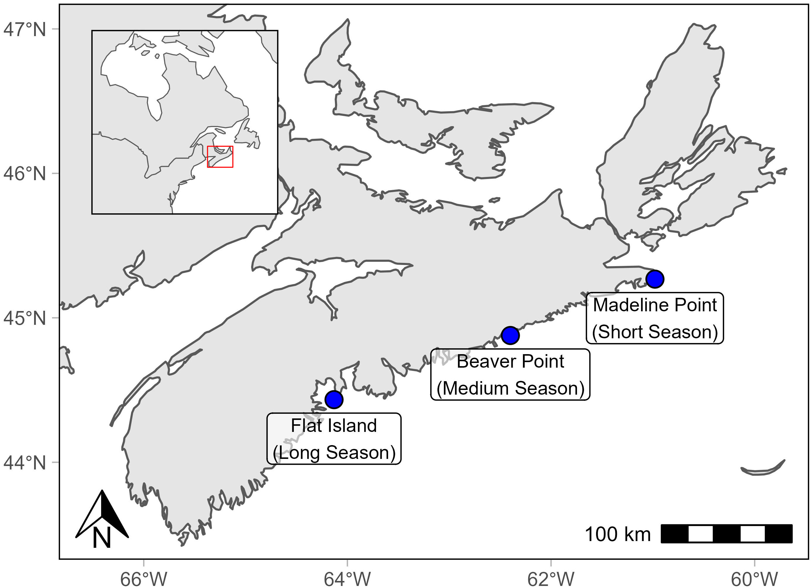
Figure 1 Stations selected to represent a short, medium, and long stocked season. Map made using the rnaturalearth and rnaturalearthhighres R packages (South, 2022a; South, 2022b).

The objectives of this study are four-fold:

1. Select three different geographic coastal locations in Nova Scotia that reflect a range of seasonal temperatures as case studies.

2. Calculate degree days within operational temperature ranges to determine the maximum practical culture duration for each location and depth.

3. Apply the TGC model to determine stocking weight required to grow to market size, under the observed degree days at each location and depth.

4. Assess the sensitivity of model output to the heat stress threshold, TGC value, and depth strata.

2 Materials and methods

2.1 Stocking weight estimation

The TGC model was applied to calculate the initial weight (i.e., stocking weight) required for salmon to grow to market size (i.e., harvest weight) given observed temperatures (Equation 2).

$\begin{array}{ll}{W}_0={(\sqrt[3]{W_t}-\frac{TGC}{1000}\ast degreedays)}^3& (2)\end{array}$

Three different TGC values were applied to model a range of growth performance. Reid et al. (2013a) calculated a TGC value of 0.30 for commercial Atlantic salmon culture in Atlantic Canada. This value was calculated across the full grow-out season, and therefore embodies inherent differences in growth rates due to life stage and environment conditions. Here, a TGC value of 0.30 was assumed to represent average growth performance, 0.25 represented slower growing, “remedial” performance, and 0.35 represented faster growing, “elite” performance. A single TGC value was applied across the entire growth period because initial weights were calculated based on the final weight, as opposed to stepwise growth stanzas. The final weight (W_t) was set to 5.5 kg, because it is a typical target market size (Njåstad, 2020; MOWI, 2021).

To account for the effects of heat stress on growth rates, it was assumed that there was no growth for 24 hours after a temperature observation ≥ 18 °C. All such heat stress observations were filtered out of the data so that growing days were used to calculate the degree days (also called growing degree days; see Table 1 for terminology). Temperatures within the 24-hour window of heat stress were not included in T_Avg, and the corresponding number of days were not included in n_days (Equation 1). While it is known that salmon can migrate vertically in response to environmental cues including temperature (Johansson et al., 2006; Johansson et al., 2009; Oppedal et al., 2011), the model is constrained to one depth for the duration of the stocked season as a simplifying assumption. It is likely that fish would avoid depths with temperatures causing heat stress when possible. In consequence, the calculated stocking weights may be conservative.

TABLE 1

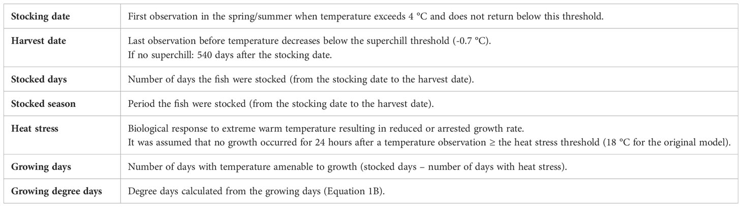
Table 1 Definition of key terms.

Model sensitivity to the heat stress threshold was assessed using the average growth model (TGC value = 0.30). The results of the original model (heat stress threshold = 18 °C) were compared to results from a model with a lower heat stress threshold (16 °C) and a higher heat stress threshold (20 °C).

The model assumes that missing temperature values are the average of the growing day temperatures (T_Avg). To check this approximation, the average of the temperature for the 24 hours before and after any data gap was calculated (T_Gap) and compared to T_Avg. To assess the sensitivity of the results when T_Gap was close to the heat stress threshold (≥ 16 °C), the analysis was repeated assuming there was no growth during the period of missing data. If the data gap represented less than 5 % of the stocked season and T_Gap was not close to the heat stress threshold, it was assumed that the missing data had negligible impact on the results.

2.2 Case study

2.2.1 Data collection

The Centre for Marine Applied Research (CMAR) has coordinated an extensive Coastal Monitoring Program in Nova Scotia, Canada since 2017 (Centre for Marine Applied Research, 2022). Through this program, temperature and other essential ocean variables (Global Ocean Observing System, 2021) are measured at locations selected in collaboration with local stakeholders (Centre for Marine Applied Research, 2022). Temperature data is collected from sub-surface “sensor strings” (Figure 2). Each string is anchored to the seafloor and suspended under constant tension from a subsurface float. Autonomous sensors are attached at various depths, typically 2, 5, 10, 15 m below the surface (at low tide), or greater depending on total depth, and most strings include a sensor just above the seabed. Several types of temperature sensors are used, including HOBO Water Temp Pro v2 U22 series (Onset, 2012), aquaMeasure DOT (InnovaSea, 2021), and Vemco VR2AR (Vemco, 2016). A sensor string is generally deployed at a sampling station 200 m – 1000 m from shore in depths up to 75 m for 6 – 12 months. Sensors record data every 1 minute to 1 hour, depending on the deployment settings. At the time of analysis, CMAR had data from 84 stations around the coast of Nova Scotia, resulting in 338 time series at various depths. Time series range from 1 month to 4.6 years, although some stations have substantial data gaps caused by battery failure, accidental and intentional vandalism, or other disruptions. This data is publicly available to visualize and download from the CMAR website (https://cmar.ca/coastal-monitoring-program/), the Nova Scotia Open Data Portal (https://data.novascotia.ca/browse?tags=coastal+monitoring+program), and the Canadian Integrated Ocean Observing System (https://catalogue.cioosatlantic.ca/dataset?q=cmar) platforms.

FIGURE 2

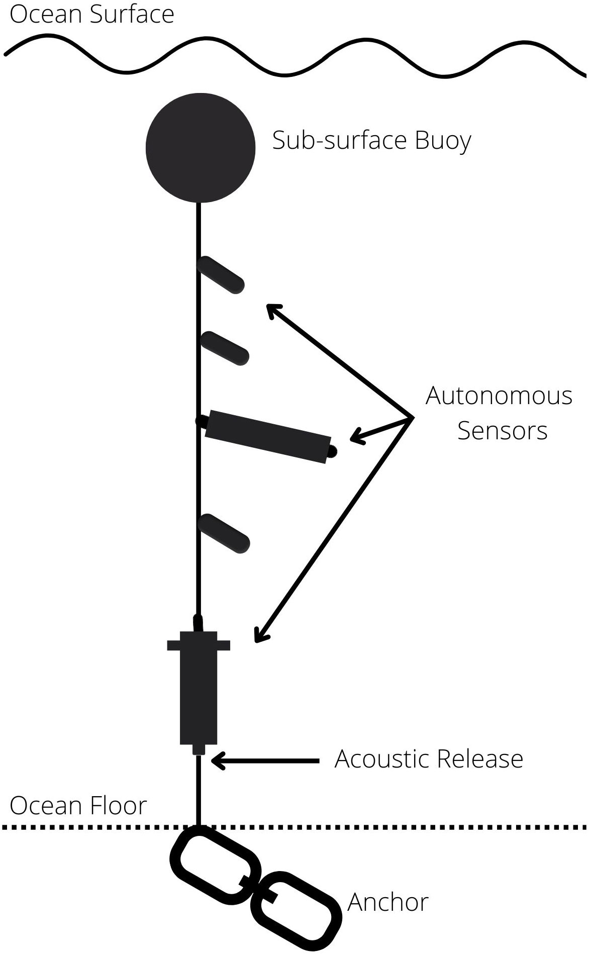
Figure 2 Example sensor string configuration (not to scale).

2.2.2 Site selection

The 338 time series of temperature at depth were carefully evaluated to select three case study stations that represent a short, medium, and long stocked season. First, stocked seasons were defined for each time series by identifying the optimal stocking and harvest dates (Table 1). The stocking date was defined as the first observation in the spring or summer when the temperature exceeded 4 °C and trended up (i.e., did not go below 4 °C), a threshold recommended by provincial fish health veterinarians in Nova Scotia to maximize fish heath and welfare. If superchill occurred the following winter, the harvest date was defined to end one minute before the first observation of superchill. If temperatures remained above this threshold, the harvest date was set at 540 days after the stocking date (i.e., a typical grow-out time). It was assumed that all fish were stocked on the stocking date and harvested on the harvest date, although in practice these events can take several weeks or months. Time series for which these dates could not be defined (e.g., data gaps) were excluded from the analysis, leaving 127 time series from 38 stations.

Next, any stocked season with more than 2 days of missing data was removed from the analysis, leaving 106 time series from 35 stations to evaluate. The durations of these remaining time series were used to inform season length categories, where “short” was less than 8.5 months; “medium” was 8.5 months to less than 17 months, and “long” was 17 months or more (i.e., seasons that did not experience superchill).

There were 12 stations with data for a short season, 10 stations with data for a medium season, and 14 stations with data for a long season. One station with data for at least 2, 5, 10 and 15 m was selected from each category to assess influence of depth on suitable temperatures. This left one station each in the short and medium season categories, and three in the long season category. Finally, the station to represent the long season was selected based on geography.

2.3 Software

All data analysis was done using R version 4.1.1. The R package tgc was developed by the authors to identify stocked seasons, filter out heat stress observations, apply the TGC model, and visualize results. The package can be installed from the GitHub repository at https://github.com/dempsey-CMAR/tgc. Data analysis code is available at https://github.com/dempsey-CMAR/TGC_Analysis.

3 Results

3.1 Stocking weight estimates

Stocking weight had an inverse relationship with growing degree days (Figure 3). For each TGC model, the stocking weight approached the harvest weight at lower degree days and approached 0 kg at very large degree days. For a given degree day, the elite growth model (TGC = 0.35) always resulted in the smallest stocking weight, and the remedial growth model (TGC = 0.25) resulted in the largest. The three models diverge the most at moderate degree days. For example, at a location with 2000-degree days, the stocking weight for the remedial model was 2.0 kg, while that of the elite model was only 1.2 kg. The modelled stocking weight decreased more rapidly for smaller number of degree days (Figure 3). For the average model, a 500-degree day increase from 1000 to 1500-degree days reduced the stocking weight by 0.88 kg (from 3.15 kg to 2.27 kg). In contrast, a 500-degree day increase from 3500 to 4000-degree days reduced the stocking weight by only 0.19 kg (from 0.37 kg to 0.18 kg).

FIGURE 3

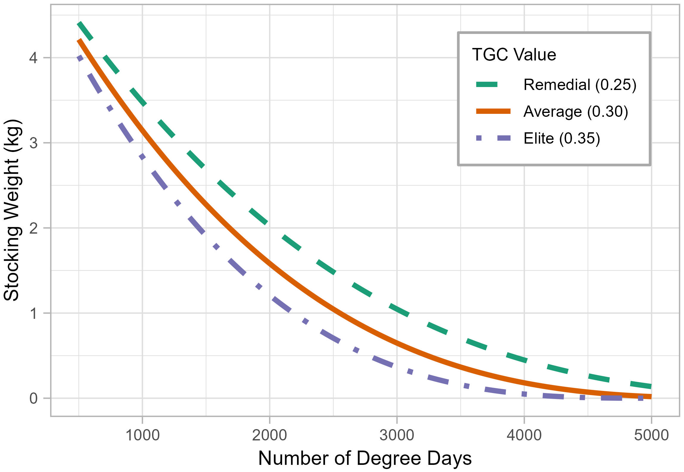
Figure 3 The thermal-unit growth coefficient model, showing the stocking weight required to grow a post-smolt salmon to market size (5.5 kg) for a given number of degree days, assuming remedial (TGC = 0.25), average (TGC = 0.30), and elite (TGC = 0.35) growth performance.

3.2 Short season: Madeline Point

The station that met the criteria to represent a short season was Madeline Point, Guysborough County, located in the north-eastern part of mainland Nova Scotia (Figure 1). The station is approximately 500 m from shore and 22 m deep, with temperature sensors at 2, 5, 10, 15, and 22 m below the surface at low tide, and a tidal range of up to 2 m. The stocked season selected for analysis was approximately 8 months long (Table 2; Figure 4A), beginning on June 17 for the shallowest depths (2 m and 5 m), followed five days later by the mid-depths (10 m and 15 m), and one additional day later for the bottom (22 m). While 22 m is an impractical culture depth for this site, it is included in this theoretical exercise for context and comparison with the other depths. The season ended in mid-February near the surface (2 m) and near the bottom (15 m and 22 m), followed a week later by the remaining strata.

TABLE 2

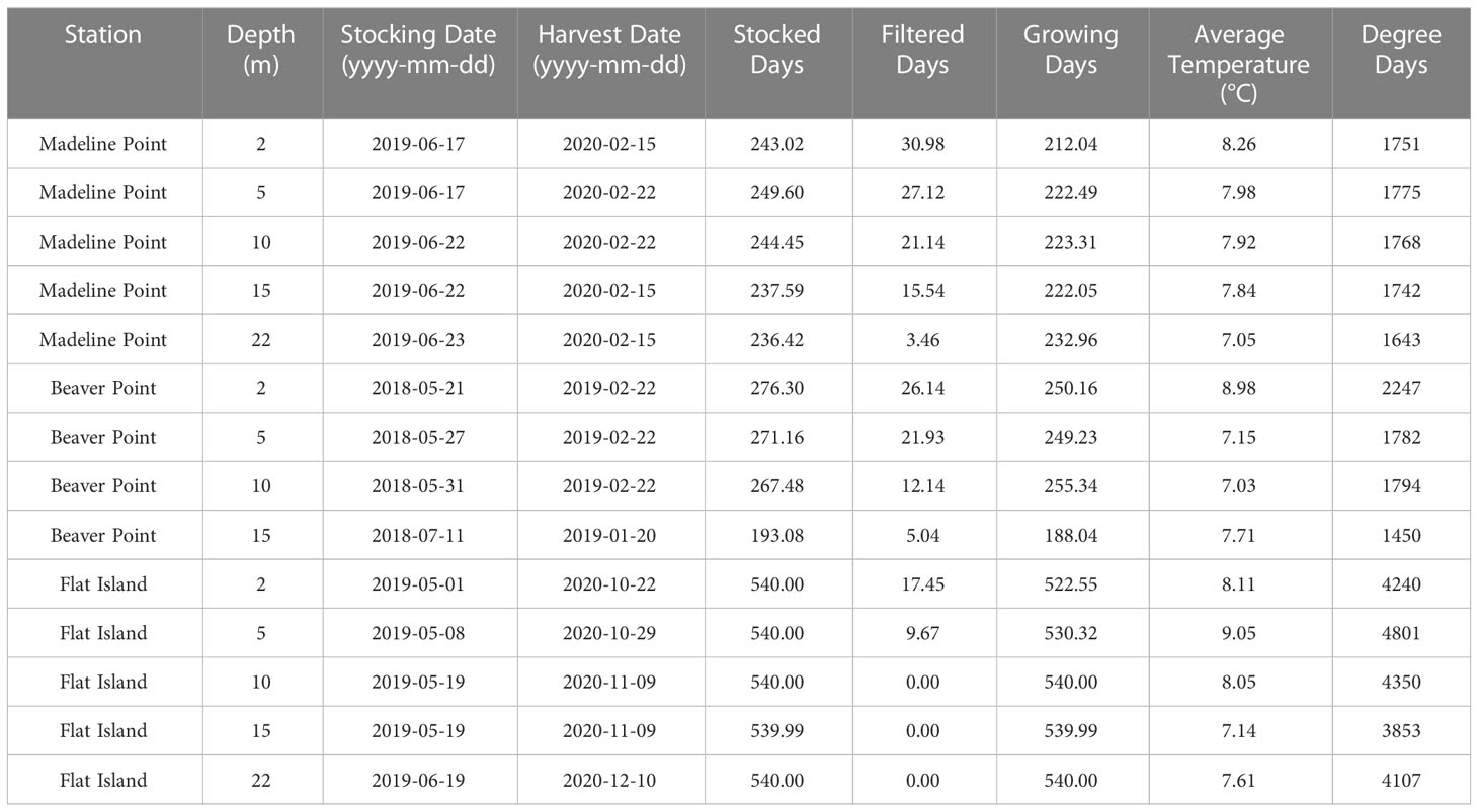
Table 2 Stocked season and degree day results for each station and depth.

FIGURE 4

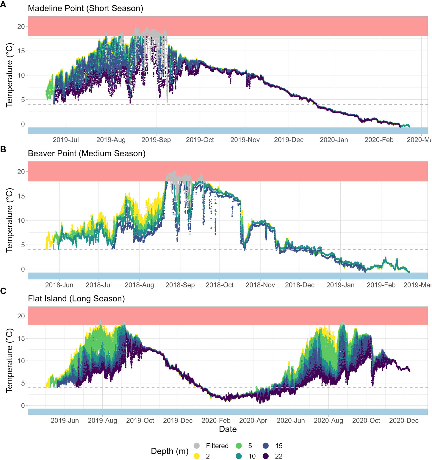
Figure 4 Temperature observations for (A) Madeline Point (short season), (B) Beaver Point (medium season), and (C) Flat Island (long season). The shaded blue area indicates the superchill threshold (-0.7 °C), the dashed grey line indicates the 4 °C threshold, and the shaded red area indicates the heat stress threshold (18 °C). Greyed observations were considered heat stress (within 24 hours of an observation ≥ 18 °C) and were filtered out of the analysis.

There was an overall increasing temperature trend in the summer, with substantial diurnal variability (Figure 4A). Limited temperature stratification occurred between 2, 5, and 10 m (average July and August temperatures for these depths were 15.3 °C, 14.6 °C, and 13.5 °C, respectively), while the bottom temperature was typically cooler (average bottom temperature was 9.2 °C). There was a distinct decreasing temperature trend throughout the fall and winter months, with no appreciable diurnal variability or stratification (average temperature ranged from 6.2 °C at 22 m to 6.6 °C at 2 m).

Heat stress events were observed at all depths (Table 2; Figure 4A). The warmest temperatures typically occurred mid-August to early September, although surface depths (2 and 5 m) experienced earlier seasonal heat stress events. These shallow depths experienced the most heat stress, with no growth assumed for 31 days at 2 m depth and 27 days at 5 m depth (approximately 13 % and 11 % of the stocked days, respectively; Figure 5). In contrast, the bottom had only two short (< 2 days) heat stress events. As a result of heat stress and growing season length, the 2 m depth had the fewest growing days, and 22 m had the most (Table 2).

FIGURE 5

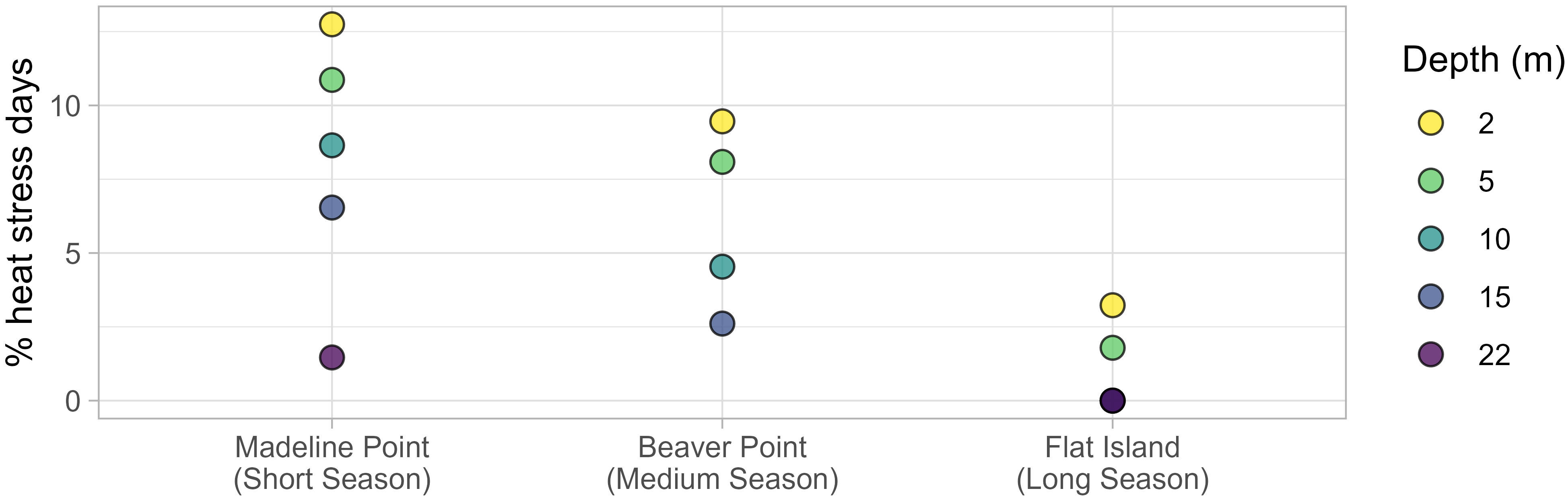
Figure 5 Percent of the stocked season at each station and depth with arrested growth caused by heat stress (≥ 18 °C). Note that there was no heat stress observed at Flat Island at 10, 15, and 22 m.

The top four depths had a very similar number of degree days (Figure 6A; Table 1). This translated to a negligible difference in the stocking weight required to grow salmon to market size at these depths (a difference of about 0.05 kg for each TGC value; Figure 6B). However, there was a substantial difference in the results between the remedial and elite models, with remedial growth requiring a stocking weight of approximately 2.3 kg and elite growth requiring a stocking weight of 1.5 kg. Near the bottom, the average temperature of the growing days was about 1 °C cooler, resulting in about 100 fewer degree-days, and a stocking weight about 0.1 kg higher than the other depths.

FIGURE 6

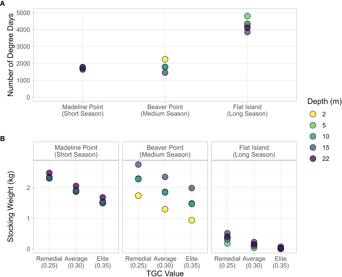
Figure 6 (A) The number of growing degree days observed at each station and depth, and (B) Stocking weight of post-smolts required to reach market size as a function of TGC value, location and depth (heat stress threshold ≥ 18 °C).

3.3 Medium season: Beaver Point

The station that met the criteria to represent a medium season was Beaver Point, located on the eastern shore of Halifax County (Figure 1). The station is approximately 300 m from shore and 15 m deep. Temperature was measured at 2, 5, 10, and 15 m below the surface at low tide, with a tidal range up to 2 m. The stocked season selected for analysis was approximately 9 months for the top three depths, beginning in late May and ending with the onset of superchill in late February (Table 2; Figure 4B). The bottom depth had a much shorter growing season of 6.4 months, because the temperature crossed the 4 °C and trending up threshold a month and a half later and experienced superchill about a month earlier than at the other depths (Table 2).

Temperature was stratified from June through to mid-August, with the average temperature at 2 m (9.8 °C) about 1 °C warmer than that at 5 m depth; in turn, the average temperature at 5 m was about 1 °C warmer than the temperatures at 10 and 15 m. Heat stress events occurred at all depths in late August, with the most prolonged at 2 m, where 26 days (9.4 % of stocked season) were assumed unsuitable for growth. In contrast, only 12 days and 5 days were considered unsuitable at 10 m and 15 m, respectively (Table 2; Figure 5). August through October was a period of rapid variability for the deeper waters. For example, in late August the temperature at 15 m dropped 13 °C over 6 days, and then rebounded 12 °C in the following 5 days. Temperature was less variable and more well-mixed in the winter months (Figure 4B), although temperature at the bottom was on average ~ 0.6 °C cooler than at the shallower depths.

The number of degree days ranged from 1450 degree days at the bottom (15 m) to 2247 degree days near the surface (2 m; Figure 6A), which translated to a difference in stocking weight of about 1 kg (Figure 6B). The smallest stocking weight occurred at 2 m, ranging from 1.7 kg for the remedial model to 0.93 kg for the elite model. The stocking weight at 5 m and 10 m had negligible differences at each TGC (~ 0.01 kg), owing to the similar number of degree days at these depths. The elite growth model at 2, 5, and 10 m required a smaller stocking weight than any of the depths for the remedial model (Figure 6B).

The 2 m temperature time series was missing 0.58 days of observations in mid-September. The average temperature for the 24 hours before and after the data gap was 17.8 °C, very close to the heat stress threshold. Assuming that there was no growth during the period of missing data (e.g., subtracting 0.58 days from n_days; Equation 1B) resulted in 5.2 fewer degree days (0.23 % fewer than the original model) and a stocking weight 0.006 kg larger (0.44 % larger for the average growth performance), which were considered negligible differences.

3.4 Long season: Flat Island

The three stations that met the criteria to represent a long season were Shad Bay, Flat Island, and Little Rafuse Island. These stations are within 35 km of each other, near the border of Halifax and Lunenburg Counties. The Flat Island station (Figure 1) was ultimately selected for analysis because it is geographically between the other two long season station candidates. The Flat Island station is approximately 22 m deep, with temperature sensors at 2, 5, 10, 15, and 22 m below the surface and a tidal range of up to 3 m. It is located approximately 5 km from shore, 2 km from Big Tancook Island, and 600 m from Flat Island.

The stocked season selected for analysis started in early May near the surface (2 and 5 m), later May at the middle depths (10 and 15 m), and mid-June at the bottom depth (22 m; Table 2). No superchill was observed in the following winter or spring, therefore the growing season lasted ~ 18 months (540 days) at each depth (Figure 4C). There was an overall increasing temperature trend at all depths in the spring and summer months, with notable stratification and diurnal variability. The temperature near the surface (2 m) was ~ 5 °C warmer than at the bottom (22 m) for the summer of 2019 and spring/summer of 2020. There was limited heat stress during this growing season, and when it occurred, it was confined to near the surface, with 17 days considered unsuitable for growth at 2 m and 9.7 days at 5 m (Table 2). Temperature was less stratified and less variable in the fall and winter months, with an overall decreasing temperature trend. Notably, there was a temperature inversion for most of mid-November through mid-March, with the coolest average temperature near the surface (3.8 °C) and the warmest average temperature near the bottom (7.6 °C; Figure 4C).

There was a range of nearly 1000-degree days for the different depths (Figure 6A). As a result of summer heat stress at the surface and the winter temperature inversion, the 5 m depth had the most degree days (4800-degree days), and the 15 m stratum had the least (3853 degree days; Table 2). The 2, 10, and 22 m depths all had relatively similar number of degree days, ranging from 4120 degree days to 4350 degree days. For the remedial growth model, this translated into modelled stocking weight ranging from 0.18 kg at 5 m to 0.52 kg at 15 m, while the results of the average model ranged from 0.034 kg to 0.23 kg. The elite model resulted in very small stocking weights, ranging from only 0.0006 kg to 0.072 kg (Figure 6B).

Delays in sensor redeployment resulted in two short gaps in the temperature data series: 1.5 days in early June 2019 (for all depths except for 22 m) and 0.2 days in November 2019. The temperature 24 hours before and after each gap is reasonably close to the average temperature (absolute difference from 0.26 °C to 2.1 °C), and the missing days represent only 0.30 % of the stocked season. The missing data was assumed to have negligible impact on the model results.

3.5 Sensitivity to heat stress threshold

3.5.1 Lower heat stress threshold (16 °C)

When the heat stress threshold was lowered to 16 °C there were ~ 20 (9 %) fewer growing days for most depths at Madeline Point and Beaver Point, which resulted in 227 (16 %) and 330 (19 %) fewer degree days, respectively. On average, this increased the stocking weight for each depth at Madeline Point by ~ 0.409 kg (22 %) and at Beaver Point by ~ 0.485 kg (26 %; Figure 7). The bottom temperature at Madeline Point rarely exceeded the 16 °C threshold, so there were only 5 fewer growing days at this depth, which required a 0.103 kg (5 %) larger post-smolt (Figure 7).

FIGURE 7

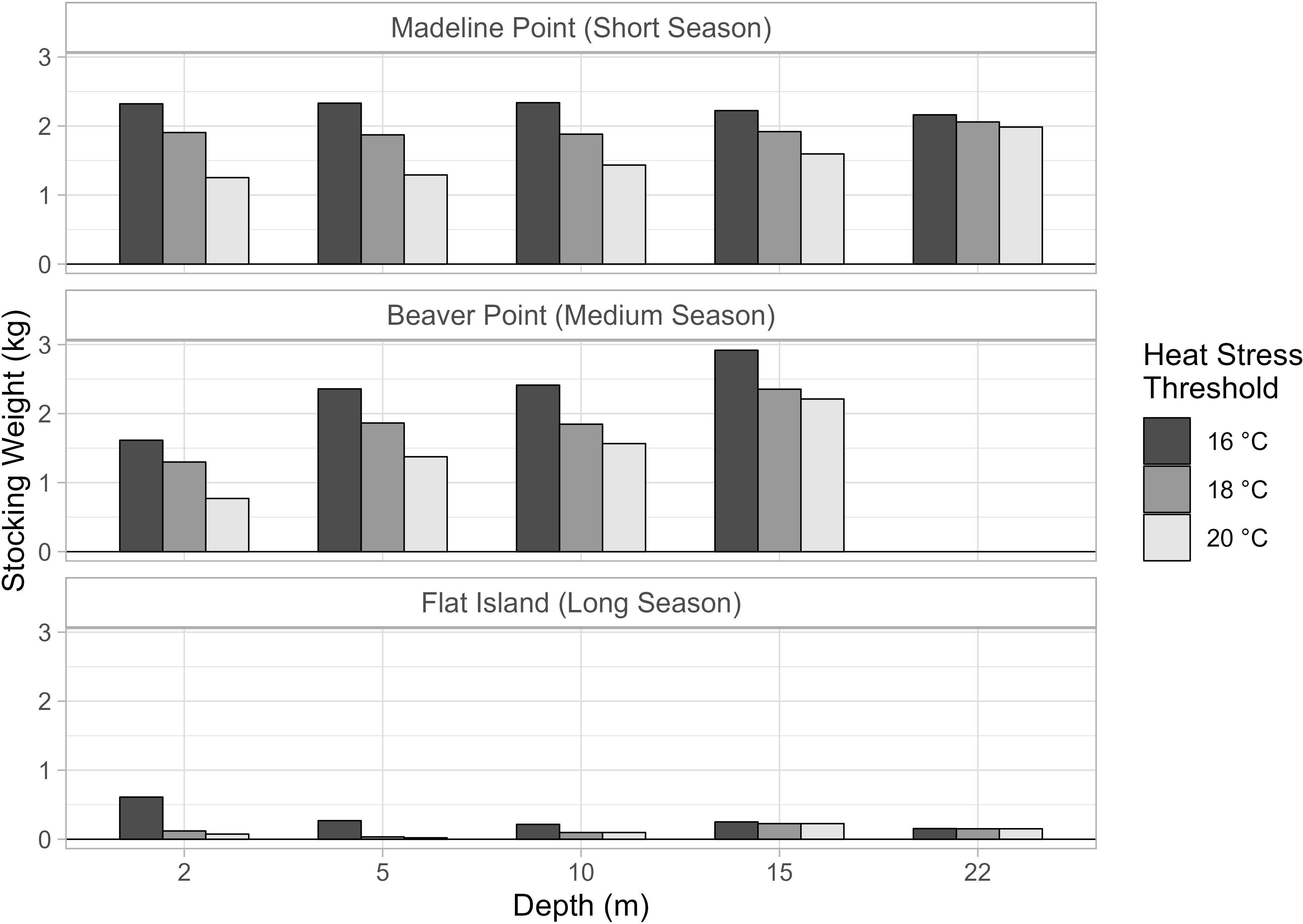
Figure 7 Stocking weight estimated from applying three different heat stress thresholds (16°C, 18°C, 20°C).

Flat Island had the largest reduction in number of growing days and degree days, particularly at the shallow depths. At 2 m, there were 88 (17 %) fewer growing days and 1184 (28 %) fewer degree days compared to the original heat stress threshold. At 5 m, there were 71 (13 %) fewer growing days and 1068 (22 %) fewer degree days. The increase in stocking weight was similar to the other stations (0.491 kg at 2 m and 0.235 kg at 5 m; Figure 7). The difference at 10 m was also substantial, with 32 (6 %) fewer growing days and 464 (11 %) fewer degree days, which translated to an increase in stocking weight of 0.118 kg (121 %). The deeper strata rarely exceeded the 16 °C threshold and had small changes in stocking weight (< 0.030 kg; < 12 %).

3.5.2 Higher heat stress threshold (20 °C)

Increasing the heat stress threshold to 20 °C was nearly equivalent to not accounting for heat stress in the model. Few observations exceeded this threshold, with only 1 day considered unsuitable for growth at Madeline Point (2 m) and 2.3 days at Beaver Point (2 m). Consequently, there were additional growing days through the whole water column at these stations, most notably for the shallower depths. At 2 m and 5 m, there were over 25 (10 %) more growing days at Madeline Point, and over 20 (9 %) additional growing days at Beaver Point. At Madeline Point, this translated into an additional 540 (30 %) degree days at 2 m, and 478 (27 %) at 5 m. Similarly at Beaver Point, there were an additional 581 (26 %) degree days at 2 m and 396 (22 %) at 5 m. No heat stress events for Flat Island were observed in this simulation, which resulted in an increase of 241 (5.7 %) degree days at 2 m and 168 (3.5 %) degree days at 5 m. No heat stress events were observed in the original model at the other depths, and so those results did not change.

The largest absolute decrease in stocking weight was for the surface depths at Madeline Point, which were 0.653 kg (34 %) and 0.581 kg (31 %) smaller than in the original model for 2 m and 5 m. This was closely followed by Beaver Point, with a reduction of 0.528 kg (40 %) and 0.489 kg (26 %) at the same depths. There was a modest reduction of < 0.050 kg for the Flat Island example.

4 Discussion

4.1 Potential for seasonal site usage

The TGC model results showed that fish weighing 1.5 – 2.5 kg can theoretically grow to market size at seasonal sites. This suggests that post-smolt stocking strategies can potentially enable use of novel sites in areas previously considered unsuitable for aquaculture because of cold winter temperatures. The modelled stocking weight was substantially larger than typical target post-smolt weights (Fish Farming Expert, 2019; Gardner Pinfold Consultants Inc., 2019; Fish Farming Expert, 2021; MOWI, 2021); however, it is technically feasible to grow salmon to this size or larger on land (Atlantic Sapphire, 2020; Sustainable Blue, 2021). Several companies have successfully moved the entire Atlantic salmon production cycle to land-based Recirculating Aquaculture System (RAS) facilities (see Table 1 of Gardner Pinfold Consultants Inc., 2019). There are still substantial challenges in the grow-out phase at these facilities, including improving fish quality, maintaining fish health, preventing fish mortalities, and managing increased costs (Calabrese, 2017; Gardner Pinfold Consultants Inc., 2019; EY, 2020; Hoel and Howell, 2021). Transferring large post-smolts to marine net-pens may offset some of these challenges, and we recommend future research into the costs and benefits of growing large post-smolts on land to stock in novel sites.

4.2 Assessing site suitability

The approach discussed here highlights that the TGC model in conjunction with high-resolution, site-specific temperature data can be a useful tool for assessing the suitability of novel areas. This temperature data can provide insight on optimal stocking and harvest dates as well as anticipated heat stress. For example, local temperature profiles were key for informing the optimal stocking date, which was related to both latitude and depth. The season began in early May at Flat Island (the most southern station) and in mid-June at Madeline Point (the most northern station), illustrating the value of using local data to inform operational decisions. Despite being on the same coast, using Flat Island data to inform the timing of stocking at Madeline Point would subject the post-smolts to 6 weeks of sub-optimal temperatures. At each station, the season started progressively later with depth, with up to 7 weeks difference between the surface and the bottom at Beaver Point. This highlights the importance of incorporating the temperature profile throughout the water column, especially for the full cage depth, into stocking decisions. Using only the surface data to inform the timing of stocking could subject the fish to potentially harmfully cold temperatures. Inter-annual temperature variation was beyond the scope of this paper, but is known to vary substantially along the coast of Nova Scotia (Centre for Marine Applied Research, 2022), and would be an important site suitability consideration.

4.2.1 Superchill

Despite seasonal occurrence of superchill along some coastal regions, it is not always predictable and is therefore a major risk for the aquaculture industry. The ability to better predict the onset of superchill would be an asset to existing and new operations, especially for potential seasonal sites. Several days or weeks warning of impending superchill would provide time to implement risk management strategies, including preparing to harvest or ceasing feeding and other activities at the cage sites (LGL Limited, 2019; Sweeney International Marine Corp, 2019). Analyzing several years of historical high-resolution data at a given location could provide useful insight into inter-annual patterns, typical and extreme events, and early warning indicators. This information could eventually feed into model forecasts of superchill extent and timing (Payne et al., 2017). Our analysis suggests that the timing of superchill is not typically related to depth, due to minimal stratification in the winter/spring, when superchill occurs. The main exception was the bottom temperatures, where superchill was observed ~ 1 month earlier at Beaver Point and ~ 1 week earlier at Madeline Point than at other depths. The occurrence of superchill at the bottom could be an early warning indicator of superchill at shallower depths where cages are located. An extensive analysis of CMAR’s Coastal Monitoring Program data to investigate whether this pattern is consistent spatially and inter-annually is recommended.

4.2.2 Heat stress

In contrast to superchill, the amount of heat stress was related to depth, with more days considered unsuitable for growth near the surface at each station (Figure 5). Surprisingly, the most heat stress was observed at Madeline Point (Table 2). This was the most northern site and had the earliest onset of superchill, and it was expected to be generally cooler than the other sites. Instead, over 8 % of the stocked days were unsuitable for growth as deep as 10 m (Figure 5). It may be worth investing in a deep net for this location so fish can avoid warm surface waters and continue to grow. In contrast, the only heat stress observed at Flat Island was near the surface, and so a typical net depth would be sufficient at this location. A major limiter of the industry in Nova Scotia is that sites are typically located in relatively shallow waters, so the net depth may be constrained by bathymetry. Site location in deeper water could enable access to a wider range of stratified temperatures, although this could require management and infrastructure changes. Long-term, high-resolution data such as those provided by the CMAR Coastal Monitoring Program can assist to inform such cost-benefit analyses.

4.3 Heat stress threshold

It is critical to choose an appropriate heat stress threshold to account for reduced growth at high temperatures. The threshold value can substantially impact the results, and an erroneous value could lead to increased economic and ecologic risks. In the original model (heat stress threshold = 18 °C), heat stress was a major impediment to growth at all three locations, particularly at shallow depths (Figure 5). When the threshold was increased to 20 °C, few observations were considered heat stress. This resulted in more growing days and higher average temperatures, and therefore required smaller stocking weights (Figure 7). If this model was used to guide stocking weight decisions, the fish may not grow to market size in the allotted season. This would be of particular concern for the seasonal sites, which are constrained by superchill, making it challenging or impossible to extend the season. For example, smolts with a stocking weight estimated from this model for Madeline Point would only grow to 4.12 kg if the stock truly experiences heat stress at 18 °C.

Lowering the heat stress threshold to 16 °C reduced the number of growing days and associated average temperatures, resulting in higher stocking weights. This model provides a more conservative estimate of the stocking weight, i.e., these large post-smolts would likely grow to market size during the defined season. However, the fish would need to grow longer on land to reach this stocking weight, which has associated costs and risks (Gardner Pinfold Consultants Inc., 2019; Hoel and Howell, 2021). For example, fish transferred to Beaver Point would require an extra 4 to 6 weeks in the land-based facility to grow to the stocking weight estimated from this model.

4.4 Growth performance

Differences in temperature driven growth performance (Handeland et al., 2004) were reflected in the remedial, average, and elite models. As expected, the elite model resulted in the smallest stocking weights for each station (Figures 3, 6). The largest discrepancy between elite and remedial models occurred for the stations with moderate degree days, Madeline Point and Beaver Point (Figure 6). There was a much higher number of degree days at Flat Island (long season), which resulted in a relatively small absolute difference in stocking weight between TGC models (Figure 6). Using a smaller TGC value (i.e., assuming a slow growth) to calculate the stocking weight is more conservative for ensuring the smolts will grow to market size during a predefined season. However, an overly conservative estimate could result in unnecessary additional time in post-smolt facilities (Gardner Pinfold Consultants Inc., 2019; Hoel and Howell, 2021).

The TGC values applied here were based on estimates from the literature, which originated from 10 – 15-year-old data (Reid et al., 2013b). Ground truthing by Cooke Aquaculture Inc.’s average production model suggested these values were reasonable. This production model aims to stock 120 g – 150 g smolts, which grow out over 22 months to a market size of 5.5 – 6 kg (Jennifer Hewitt, Cooke Aquaculture Inc., personal communication October 2022). Using these initial and final weights and temperature data from the example stations, TGC values ranging from 0.234 – 0.263 were calculated (equation 1), which correspond with the remedial growth performance TGC. The elite growth performance value was derived based on the assumption that selective breeding suggests improved growth rate by about 10 % per generation (Gjøen and Bentsen, 1997; Gjedrem, 2000; Thorarensen and Farrell, 2011). This highlights the need for updated commercial TGC coefficients for Atlantic salmon grown in marine net-pens to improve confidence in the model results.

Determining whether elite performing stocks grow faster than the average and remedial performing salmon at high temperatures would be relevant for breeding programs. Tolerance to high temperature, often measured using the critical thermal maximum, varies between families (Anttila et al., 2013). Moreover, it has been shown that tolerance to heat stress, which is a heritable trait in salmon, and growth rate may be inversely correlated, suggesting that simultaneous selection for both traits is unattainable (Debes et al., 2021).

4.5 Degree days drivers and outcomes

Degree days are a key metric for modelling growth of ectotherms, accounting for both growing time and temperature. Our results reinforce that both degree day factors, n_days and T_Avg, are important drivers. For example, Flat Island and Madeline Point had similar average temperatures at 10 m; however, Flat Island had more than double the number of growing days (Table 2). The resulting stocking weights at Flat Island were 7 (remedial model) to 100 (elite model) times smaller than at Madeline Point (Figure 6). In this analysis, n_days was adjusted to account for reduced growth rates caused by heat stress. Other factors that affect growth rates (e.g., no-feed events, photoperiod influence) are assumed to be accounted for in the TGC value, which is derived from historical production data over the growth period. There is no historical production data for the novel locations assessed in this study, and so the application of remedial, average, and elite performing TGC values aimed to account for a range of potential influences to growth performance.

The Beaver Point and Madeline Point results illustrate the importance of temperature. At 5 m and 10 m, there were ~ 30 more growing days at Beaver Point (Table 2). A naïve prediction would be that smaller smolts could be stocked at Beaver Point because they have more time for grow-out. However, the average temperature of the growing days at Madeline Point was 0.8 °C warmer that that at Beaver Point, resulting in very similar stocking weights for both locations (Figure 6). It is therefore critical to have high-quality, ideally site-specific temperature data for useful estimates from the TGC model.

Under the TGC model, initial weight is related to the number of degree days through a non-linear (cubic) relationship (Equation 2), which can also lead to unintuitive results. For example, an absolute change in the degree days can result in a differential change in initial weight (Figure 3). A wide range in the number of degree days at Beaver Point results in a ~ 1 kg difference in stocking weight between the surface and the bottom depths. Flat Island had a similar range of degree days at depth, but a substantially smaller range of stocking weights, particularly for the elite model (Figure 6). This is because the range of degree days at Beaver Point (1450 – 2247 degree days) corresponds to a relatively steep part of the curve shown in Figure 3. In contrast, the number of degree days at Flat Island is substantially higher (3858 – 4801 degree days) and corresponds to a flat part of the curve, most notably for the elite model. These results illustrate that additional degree days at a location may not translate to appreciable differences in stocking weight. We recommend consulting a stocking weight-degree day curve (Figure 3) to inform cost-benefit of expanding to an additional depth or location with more degree days.

The Flat Island example also highlights that TGC results should be interpreted carefully and in context, especially at extreme degree day values. At high degree days the modelled stocking weight approaches zero and can even become negative (Figure 3). At Flat Island, the stocking weight of the elite growth model for all depths was less than 120 g, a typical size for smolt stocked in Nova Scotia (Jennifer Hewitt, Cooke Aquaculture, personal communication, October 2022). The stocking weight at 5 m was only 0.6 g, which is about the size of a fry and would not survive in the marine environment.

At very small degree days, the modelled stocking weight will approach market size (Figure 3). It may be impractical to transport such large fish to ocean net-pens for the remaining short grow-out period. Before modelling, it is important to identify operational thresholds including the minimum and maximum acceptable smolt size, and to inspect the results accordingly.

5 Conclusion

The method and results presented here suggest that further investigations into large post-smolt stocking to circumvent short periods of cold temperatures are warranted. The method is straightforward to apply to any potential site with observed temperature data. We recommend high-resolution, long-term, and site-specific temperature data for estimates of stocking and harvest dates and heat stress. This method could be easily adopted for other species with known TGC values and heat stress thresholds.

Data availability statement

Publicly available datasets were analyzed in this study. This data can be found here: Madeline Point: https://data.novascotia.ca/Nature-and-Environment/Guysborough-County-Water-Quality-Data/eb3n-uxcb Beaver Point: https://data.novascotia.ca/Nature-and-Environment/Halifax-County-Water-Quality-Data/x9dy-aai9 Flat Island: https://data.novascotia.ca/Nature-and-Environment/Lunenburg-County-Water-Quality-Data/eda5-aubu.

Author contributions

GR, DD, and LLM conceived of and designed the analysis. DD wrote the code, interpreted results, and drafted the manuscript. All authors contributed to the article and approved the submitted version.

Conflict of interest

Author RC is employed by C&H Aquatic and Laboratory Veterinary Services Ltd. Author AD is employed by Aquaculture Nutrition Services Inc. Author JR is employed by System Science Applications Inc.

The remaining authors declare that the research was conducted in the absence of any commercial or financial relationships that could be construed as a potential conflict of interest.

Publisher’s note

All claims expressed in this article are solely those of the authors and do not necessarily represent those of their affiliated organizations, or those of the publisher, the editors and the reviewers. Any product that may be evaluated in this article, or claim that may be made by its manufacturer, is not guaranteed or endorsed by the publisher.

References

Anttila K., Dhillon R. S., Boulding E. G., Farrell A. P., Glebe B. D., Elliott J. A., et al. (2013). Variation in temperature tolerance among families of Atlantic salmon (Salmo salar) is associated with hypoxia tolerance, ventricle size and myoglobin level. J. Exp. Biol. 216 (7), 1183–1190. doi: 10.1242/jeb.080556

PubMed Abstract | CrossRef Full Text | Google Scholar

Atlantic Sapphire (2020). Annual report 2020.

Google Scholar

Aunsmo A., Krontveit R., Valle P. S., Bohlin J. (2014). Field validation of growth models used in Atlantic salmon farming. Aquaculture 428–429 (0), 249–257. doi: 10.1016/j.aquaculture.2014.03.007

CrossRef Full Text | Google Scholar

Calabrese S. (2017). Environmental and biological requirements of post-smolt Atlantic salmon (Salmo salar l.) in closed-containment aquaculture systems (PhD, University of Bergen).

Google Scholar

CBC (2015). Nova Scotia Aquaculture fish killed by superchilled water (Nova Scotia, Canada: Canadian Broadcasting Corporation (CBC). Available at: https://www.cbc.ca/news/canada/nova-scotia/nova-scotia-aquaculture-fish-killed-by-superchilled-water-1.2980172

Google Scholar

Centre for Marine Applied Research (2022). Coastal monitoring program (Dartmouth, Nova Scotia: Centre for Marine Applied Research (CMAR). Available at: https://cmar.ca/coastal-monitoring-program/.

Google Scholar

Cho C. Y., Bureau D. P. (1998). Development of bioenergetic models and the fish-PrFEQ software to estimate production, feeding ration and waste output in aquaculture. Aquat. Living Resour. 11 (4), 199–210. doi: 10.1016/S0990-7440(98)89002-5

CrossRef Full Text | Google Scholar

Chowdhury M. A. K., Siddiqui S., Hua K., Bureau D. P. (2013). Bioenergetics-based factorial model to determine feed requirement and waste output of tilapia produced under commercial conditions. Aquaculture 410-411, 138–147. doi: 10.1016/j.aquaculture.2013.06.030

CrossRef Full Text | Google Scholar

Debes P. V., Solberg M. F., Matre I. H., Dyrhovden L., Glover K. A. (2021). Genetic variation for upper thermal tolerance diminishes within and between populations with increasing acclimation temperature in Atlantic salmon. Heredity 127 (5), 455–466. doi: 10.1038/s41437-021-00469-y

PubMed Abstract | CrossRef Full Text | Google Scholar

Dumas A., France J., Bureau D. P. (2007). “Evidence of three growth stanzas in rainbow trout (Oncorhynchus mykiss) across life stages and adaptation of the thermal-unit growth coefficient,” in The XII international symposium on fish nutrition and feeding (Elsevier).

Google Scholar

Dumas A., France J., Bureau D. (2010). Modelling growth and body composition in fish nutrition: where have we been and where are we going? Aquacult. Res. 41 (2), 161–181. doi: 10.1111/j.1365-2109.2009.02323.x

CrossRef Full Text | Google Scholar

Dunagan C. (2021) Taking the temperature of salmon. Available at: https://www.eopugetsound.org/magazine/taking-temperature-salmon.

Google Scholar

Elliott J. M., Elliott J. A. (2010). Temperature requirements of Atlantic salmon Salmo salar, brown trout Salmo trutta and Arctic charr Salvelinus alpinus: predicting the effects of climate change. J. Fish Biol. 77, 1793–1817. doi: 10.1111/j.1095-8649.2010.02762.x

PubMed Abstract | CrossRef Full Text | Google Scholar

Elliott J. M., Hurley M. A. (2000). Daily energy intake and growth of piscivorous brown trout, salmo trutta. Freshw. Biol. 44 (2), 237–245. doi: 10.1046/j.1365-2427.2000.00560.x

CrossRef Full Text | Google Scholar

EY (2020). The Norwegian aquaculture analysis 2020.

Google Scholar

Feindel N., Cooper L., Trippel E., Blair T. (2013). “Climate change and marine aquaculture in Atlantic Canada and Quebec,” in Climate change impacts, vulnerabilities and opportunities analysis of the marine Atlantic basin. vol. 3012 of Canadian manuscript reports of fisheries and aquatic sciences. Eds. Shackell N. L., Greenan B., Pepin P., Chabot D., Warburton A. (Nova Scotia: Fisheries and Oceans Canada (DFO), Ocean and Ecosystem Sciences Division, Bedford Institute of Oceanography), 195–255.

Google Scholar

Fisheries and Oceans Canada (2022). Fallowing as a tool for disease mitigation in marine finfish facilities in British Columbia (Pacific Region: Canadian Science Advisory Secretariat Science Response 2022/023).

Google Scholar

Fish Farming Expert (2019) Huon bids to cut time at sea with 1kg nursery salmon. Available at: https://www.fishfarmingexpert.com/article/huon-bids-to-cut-time-at-sea-with-1kg-plus-nursery-salmon/ (Accessed 2021).

Google Scholar

Fish Farming Expert (2020) Canadian Bigger smolts project given $1.8m funding. Available at: https://www.fishfarmingexpert.com/article/canadian-bigger-smolts-project-given-18m-funding/ (Accessed 2021).

Google Scholar

Fish Farming Expert (2021) Half-kilo smolts will halve time at sea for Scottish salmon company fish. Available at: https://www.fishfarmingexpert.com/article/half-kilo-smolts-will-halve-time-at-sea-for-scottish-salmon-co-fish/ (Accessed 2021).

Google Scholar

Gamperl A. K., Ajiboye O. O., Zanuzzo F. S., Sandrelli R. M., Peroni E., Beemelmanns A. (2020). The impacts of increasing temperature and moderate hypoxia on the production characteristics, cardiac morphology and haematology of Atlantic salmon (Salmo salar). Aquaculture 519, 734874. doi: 10.1016/j.aquaculture.2019.734874

CrossRef Full Text | Google Scholar

Gamperl A., Zrini Z., Sandrelli R. (2021). Atlantic Salmon (Salmo salar) cage-site distribution, behavior, and physiology during a Newfoundland heat wave. Front. Physiol. 12. doi: 10.3389/fphys.2021.719594

CrossRef Full Text | Google Scholar

Gardner Pinfold Consultants Inc. (2019). State of salmon aquaculture technologies.

Google Scholar

Gjøen H. M., Bentsen H. B. (1997). Past, present, and future of genetic improvement in salmon aquaculture. ICES J. Mar. Sci. 54 (6), 1009–1014. doi: 10.1016/s1054-3139(97)80005-7

CrossRef Full Text | Google Scholar

Gjedrem T. (2000). Genetic improvement of cold-water fish species. Aquacult. Res. 31 (1), 25–33. doi: 10.1046/j.1365-2109.2000.00389.x

CrossRef Full Text | Google Scholar

Global Ocean Observing System (2021) Essential ocean variables. Available at: https://www.goosocean.org/index.php?option=com_content&view=article&id=14&Itemid=114 (Accessed June 1, 2021).

Google Scholar

Grieg Seafood (2020) Our impact: more sustainable farming with post smolt. Available at: https://griegseafood.com/our-impact-post-smolt.

Google Scholar

Handeland S. O., Imsland A. K., Stefansson S. O. (2008). The effect of temperature and fish size on growth, feed intake, food conversion efficiency and stomach evacuation rate of Atlantic salmon post-smolts. Aquaculture 283 (1), 36–42. doi: 10.1016/j.aquaculture.2008.06.042

CrossRef Full Text | Google Scholar

Handeland S. O., Wilkinson E., Sveinsbø B., McCormick S. D., Stefansson S. O. (2004). Temperature influence on the development and loss of seawater tolerance in two fast-growing strains of Atlantic salmon. Aquaculture 233 (1), 513–529. doi: 10.1016/j.aquaculture.2003.08.028

CrossRef Full Text | Google Scholar

Hoel T., Howell D. (2021). Land-based salmon farming: key investment considerations. Available at: https://thefishsite.com/articles/land-based-salmon-farming-key-investment-considerations

Google Scholar

Holland J. (2021) Mowi Scotland plans new post-smolt site. Available at: https://www.seafoodsource.com/news/aquaculture/mowi-scotland-plans-new-post-smolt-site (Accessed April 26, 2022).

Google Scholar

InnovaSea (2021). Realtime monitoring product manual.

Google Scholar

Iwama G. K., Tautz A. F. (1981). A simple growth model for salmonids in hatcheries. Can. J. Fish. Aquat. Sci. 38 (6), 649–656. doi: 10.1139/f81-087

CrossRef Full Text | Google Scholar

Jobling M. (1981). Temperature tolerance and the final preferendum–rapid methods for the assessment of optimum growth temperatures. J. Fish Biol. 19 (4), 439–455. doi: 10.1111/j.1095-8649.1981.tb05847.x

CrossRef Full Text | Google Scholar

Jobling M. (2003). The thermal growth coefficient (TGC) model of fish growth: a cautionary note. Aquacult. Res. 34 (7), 581–584. doi: 10.1046/j.1365-2109.2003.00859.x

CrossRef Full Text | Google Scholar

Johansson D., Ruohonen K., Juell J.-E., Oppedal F. (2009). Swimming depth and thermal history of individual Atlantic salmon (Salmo salar l.) in production cages under different ambient temperature conditions. Aquaculture 290 (3–4), 296–303. doi: 10.1016/j.aquaculture.2009.02.022

CrossRef Full Text | Google Scholar

Johansson D., Ruohonen K., Kiessling A., Oppedal F., Stiansen J.-E., Kelly M., et al. (2006). Effect of environmental factors on swimming depth preferences of Atlantic salmon (Salmo salar l.) and temporal and spatial variations in oxygen levels in sea cages at a fjord site. Aquaculture 254 (1–4), 594–605. doi: 10.1016/j.aquaculture.2005.10.029

CrossRef Full Text | Google Scholar

LGL Limited (2019). Placentia bay Atlantic salmon aquaculture project environmental effects monitoring plan: climate and weather. LGL Rep. FA0159F. Rep. by LGL Limited, St. John’s, NL for Grieg NL, Marystown, NL. 11 p.

Google Scholar

Mayer L. (2022). Post-smolt initiatives are a’ very safe bet,’ will drive growth for farmers. SalmonBusiness. Available at: https://salmonbusiness.com/post-smolt-initiatives-are-a-very-safe-bet-will-drive-growth-for-farmers/?utm_source=SalmonBusiness+Subscribers&utm_campaign=21d11db504-RSS_EMAIL_CAMPAIGN_SalmonB&utm_medium=email&utm_term=0_dddf4df39a-21d11db504-101480067

Google Scholar

Morita K., Fukuwaka M. A., Tanimata N., Yamamura O. (2010). Size-dependent thermal preferences in a pelagic fish. Oikos 119 (8), 1265–1272. doi: 10.1111/j.1600-0706.2009.18125.x

CrossRef Full Text | Google Scholar

MOWI (2021). Salmon farming industry handbook. Available at: https://www.intrafish.com/prices/farmed-salmon-prices-continue-freefall-were-losing-millions/2-1-829675

Google Scholar

Njåstad M. (2020). Farmed salmon prices continue freefall: 'We're losing millions'. Intrafish.

Google Scholar

Onset (2012). HOBO® water temp pro v2 (U22-001) manual.

Google Scholar

Oppedal F., Dempster T., Stien L. H. (2011). Environmental drivers of Atlantic salmon behaviour in sea-cages: a review. Aquaculture 311 (1–4), 1–18. doi: 10.1016/j.aquaculture.2010.11.020

CrossRef Full Text | Google Scholar

Payne M. R., Hobday A. J., MacKenzie B. R., Tommasi D., Dempsey D. P., Fässler S. M. M., et al. (2017). Lessons from the first generation of marine ecological forecast products. Front. Mar. Sci. 4. doi: 10.3389/fmars.2017.00289

CrossRef Full Text | Google Scholar

Pörtner H.-O., Peck M. A. (2010). Climate change effects on fishes and fisheries: towards a cause-and-effect understanding. J. Fish Biol. 77 (8), 1745–1779. doi: 10.1111/j.1095-8649.2010.02783.x

PubMed Abstract | CrossRef Full Text | Google Scholar

Reid G. K., Chopin T., Robinson S. M. C., Azevedo P., Quinton M., Belyea E. (2013a). Weight ratios of the kelps, Alaria esculenta and Saccharina latissima, required to sequester dissolved inorganic nutrients and supply oxygen for Atlantic salmon, Salmo salar, in integrated multi-trophic aquaculture systems. Aquaculture 408/409 (0), 34–46. doi: 10.1016/j.aquaculture.2013.05.004

CrossRef Full Text | Google Scholar

Reid G. K., Forster I., Cross S., Pace S., Balfry S., Dumas A. (2017). Growth and diet digestibility of cultured sablefish: implications for nutrient waste production and integrated multi-trophic aquaculture. Aquaculture. 470, 223–229. doi: 10.1016/j.aquaculture.2016.12.010

CrossRef Full Text | Google Scholar

Reid G. K., Lefebvre S., Filgueira R., Robinson S. M. C., Broch O. J., Dumas A., et al. (2020). Performance measures and models for open-water integrated multi-trophic aquaculture. Rev. Aquacult. 12 (1), 47–75. doi: 10.1111/raq.12304

CrossRef Full Text | Google Scholar

Reid G. K., Robinson S. M. C., Chopin T., MacDonald B. A. (2013b). Dietary proportion of fish culture solids required by shellfish to reduce the net organic load in open-water integrated multi-trophic aquaculture: a scoping exercise with cocultured Atlantic salmon (Salmo salar) and blue mussel (Mytilus edulis). J. Shellfish Res. 32, 509–517. doi: 10.2983/035.032.0230

CrossRef Full Text | Google Scholar

Saunders R. L. (1995). “Salmon aquaculture: present status and prospects for the future,” in Cold-water aquaculture in Atlantic Canada, 2nd Edition. Ed. Bogden A. D. (Moncton, N.B., Canada: Canadian Institute for Research on Regional Development).

Google Scholar

Saunders R. L., Muise B. C., Henderson E. B. (1975). Mortality of salmonids cultured at low temperature in sea water. Aquaculture 5 (3), 243–252. doi: 10.1016/0044-8486(75)90002-2

CrossRef Full Text | Google Scholar

South A. (2022a). "rnaturalearth: world map data from natural earth".

Google Scholar

South A. (2022b). "rnaturalearthhires: high resolution world vector map data from natural earth used in rnaturalearth".

Google Scholar

Sustainable Blue (2021) Introducing RAS, our proprietary recirculating aquaculture system. Available at: https://www.sustainableblue.com/innovation.

Google Scholar

Sweeney International Marine Corp (2019). "Liverpool bay development plans".

Google Scholar

Thorarensen H., Farrell A. P. (2011). The biological requirements for post-smolt Atlantic salmon in closed-containment systems. Aquaculture 312 (1), 1–14. doi: 10.1016/j.aquaculture.2010.11.043

CrossRef Full Text | Google Scholar

Thyholdt S. B. (2014). The importance of temperature in farmed salmon growth: regional growth functions for Norwegian farmed salmon. Aquacult. Economics Manage. 18, 189–204. doi: 10.1080/13657305.2014.903310

CrossRef Full Text | Google Scholar

Vemco (2016). "VR2AR user manual".

Google Scholar

Vikesa V., Nankervis L., Hevroy E. M. (2017). Appetite, metabolism and growth regulation in Atlantic salmon (Salmo salar l.) exposed to hypoxia at elevated seawater temperature. Aquacult. Res. 48 (8), 4086–4101. doi: 10.1111/are.13229

CrossRef Full Text | Google Scholar

Withers P. (2021). Cooke Aquaculture proposes $58M salmon hatchery on digby neck. CBC News.

Google Scholar