An assessment of the LICOM Forecast System under the IVTT class4 framework

1 Introduction

The safety and efficiency of marine activities, such as marine transportation, oil, and gas industry, military operations, fishery, and marine search and rescue activities, necessitates high-quality ocean reanalysis and short-range predictions of the ocean state at both global and regional scales (Schiller et al., 2008). The first operational global or basin-scale ocean forecast system was developed in the late 1990s when oceanic observations, high-resolution satellite data, high-performance computers, and advanced ocean data assimilation methods were routinely available. Due to the remarkable growth in supercomputing resources and the development of ocean observation systems, the prediction systems of global ocean forecasting were significantly improved from several points of view, including the sensibly increased their resolution, the increased complexity of the models, more processes resolved by the system (Tonani et al., 2015).

Operational marine forecast using global eddy-resolving systems has been conducted since 2010 by three national ocean centers, including the Mercator Océan in France, the Naval Research Laboratory (NRL), and the National Centers for Environmental Prediction (NCEP) in the US (Tonani et al., 2015). In China, the Ocean Forecast System (OFS) has been developed into eddy-resolving in recent years. A global eddy-resolving forecast system based on NEMO (Nucleus for European Modelling of the Ocean, Gurvan et al., 2017) of 1/12° is now operating in the National Marine Environmental Forecasting Center (NMEFC) and a new ocean forecast system based on Mass Conservation Ocean Model (MaCOM) with 10km resolution was published in 2022. The OFS based on the surface wave-tide-circulation coupled ocean model developed by the First Institute of Oceanography (FIO-COM) was published in 2018 (Qiao et al., 2019), which has a resolution of 1/10°. The Institute of Atmospheric Physics of Chinese Academy of Sciences developed a new forecast system named LFS (LICOM Forecast System, Liu et al., 2023) based on the eddy-resolving ocean circulation model - LICOM version 3 (LICOM3, Yu et al., 2018; Lin et al., 2020).

As LFS is a novel ocean forecast system, a comprehensive evaluation is essential. The primary objective of this study is to evaluate the forecast results from LFS against the observations and compare them with other forecast systems based on IVTT Class 4 framework. The IVTT, initiated by GODAE Ocean View, focuses on the inter-comparison between the systems by using a standard set of observations as a proxy for the truth. The IVTT framework includes four classes of comparisons (Class 1-4), with Class 4 contains a set of metrics designed for forecast verification (Ryan et al., 2015). The metrics include bias, the root mean square error (RMSE), the anomaly correlation, and the skill score for global and regional features. Within the framework of IVTT Class4, forecasted physical parameters of SST (sea surface temperature), SSH (sea level height) and the temperature and salinity in the sub-surface can be interpolated and compared to the in-situ observations. These are also the method employed in the present study.

This paper is organized as follows. Section 2 details the basic configuration of LFS and methods, while Section 3 presents the evaluation of the results. Concluding remarks and discussions are summarized in section 4.

2 System and methods

2.1 LICOM Forecast System

The LFS, or LICOM Forecast System, is developed based on LICOM3 and incorporates several enhancements to improve its performance. The dynamical framework adopts generalized orthogonal coordinates, and the tripolar grid described by Murray (1996) is applied (Yu et al., 2018). To refine the physical processes, the internal tide parameterization from St. Laurent et al. (2002) and the thickness diffusivities from Ferreira et al. (2005) are introduced (Yu et al., 2017; Li et al., 2020). Additionally, the flux coupler is upgraded to NCAR flux coupler version 7, enhancing the model’s flexibility for coupling and facilitating high-resolution simulations (Lin et al., 2016).

The horizontal resolution of the LFS remains consistent with that of LICOM3, featuring 3600×2302 horizontal grids (1/10°) and 55 vertical levels. The average zonal grid distance is approximately 6.9 km globally, about 11 km at the equator, and progressively decreases to 2.7 km at the high-latitude around Antarctic. The eta coordinate is employed vertically; 42 layers configured in the upper 1000 meters. Furthermore, a thermodynamic sea-ice model, CICE4 (Community Ice CodE version 4, Hunke and Lipscomb, 2010), is coupled with the LICOM3 ocean model through the flux coupler. Consequently, the LFS is capable of forecasting sea ice conditions.

In the current version of LFS, the assimilation module is not yet fully developed; therefore, the nudging method is employed to obtain the initial state for forecasting. The simulation, which provides the initial state, is referred to as the analysis experiment (ExpA). Within ExpA, the simulated temperature and salinity in LFS are restored to the temperature and salinity values from Mercator Océan PSY4 analysis (Lellouche et al., 2018), respectively. To preserve the influence of mesoscale eddies, a nudging time scale to 5 days is set for the upper 2000 meters and gradually relaxed to 20 days down to the depth of 5600 meters. Figure 1 displays a comparison of SST and SSH between the LFS and Mercator PSY4 for the period of June 1^st to December 31^st, 2014. Employing the nudging method, the LFS simulates a spatial distribution of SST that closely resembles that of the Mercator PSY4 analysis (Figures 1A, B). A slightly warmer SST is observed in the Indian Ocean, whereas a cooler SST is evident in the eastern Pacific (Figure 1C). The global standard deviation (STD) is 0.07°C. In ExpA, the simulated SSH also aligns well with the Mercator PSY4 analysis, with a global STD of 0.001 m (Figures 1D–F). The results of ExpA suggest that the nudging method could serve as an effective approach for providing the intimal state necessary for forecasting.

FIGURE 1

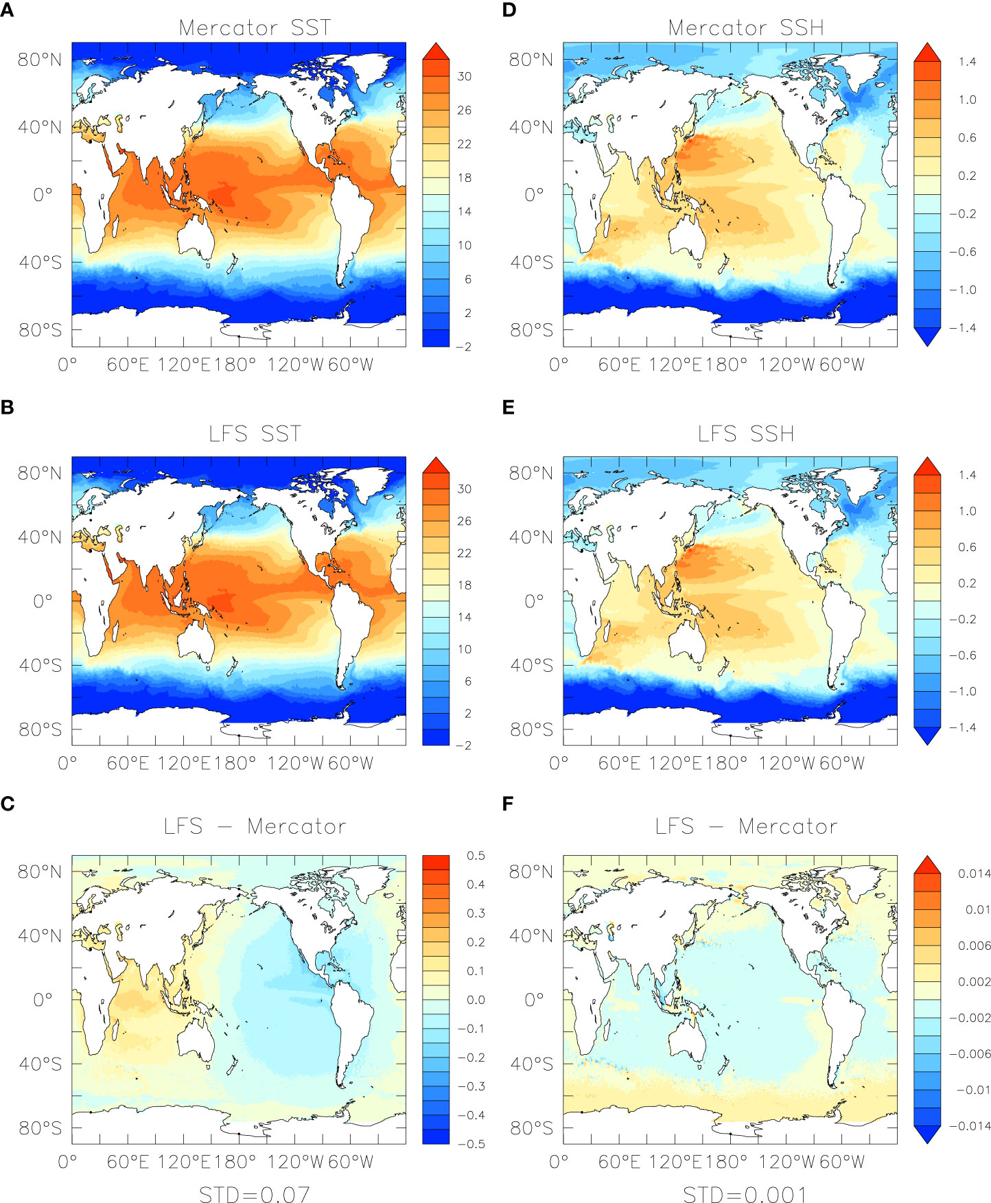
Figure 1 (A) The mean sea surface temperature (SST, °C) and (D) the mean sea surface height (SSH, m) for the Mercator Océan PSY4 during the 1^st Jun – 31^st Dec, 2014. (B, E) are the same as (A, D) but for the analysis experiment ExpA. (C, F) show their differences.

In the forecasting experiment (ExpF), initial values derived from ExpA are utilized, while the atmospheric variables and land surface runoff from the Global Forecast System (GFS) serve as external forcing to drive the LFS. The atmospheric variables include total precipitation, downward and upward shortwave radiation at the surface, downward longwave radiation, sea level pressure, 10-meter zonal/meridional wind component, air temperature and specific humidity at 2 meters. The atmospheric variables and runoff are pre-processed and subsequently read by the atmosphere and land data models in Coupler 7, which then provides the forcing. This forcing is interpolated onto the ocean model grid, and the fluxes are calculated to drive the forecast system. The air-sea fluxes are computed using the Coordinated Ocean Reference Experiments (CORE) bulk formula (Large and Yeager, 2004). In this study, the prediction spans from June 1^st to December 31^st, 2014, with a forecast time of six days. The forecast variables comprise daily averaged outputs of SST, temperature, salinity, ocean currents, and sea level height.

2.2 Data and methods

In this study, we adopt the metrics defined in Class 4 and validate the LFS by using the observations organized within the IVTT framework. Evaluation metrics include bias, RMSE, anomaly correlation, and forecast skill scores. The IVTT Class 4 reference datasets of 2014 include six forecast systems from five research organizations, which includes the Forecast Ocean Assimilation Model (FOAM) from Met Office, the operational ocean analysis and forecasting systems (PSY3 and PSY4) from Mercator Océan, the Global Ice Ocean Prediction System (GIOPS) from Environment Canada, the Real-Time Ocean Forecast System (RTOFS) from NCEP/NWS/NOAA, the Ocean Model Analysis and Prediction System (Ocean-MAPS) from Australian Bureau of Meteorology. Details regarding these systems are listed in Table 1. All the systems feature a six-day forecast periods, and the forecasts from June 1^st to December 31^st are employed for the LFS validation.

TABLE 1

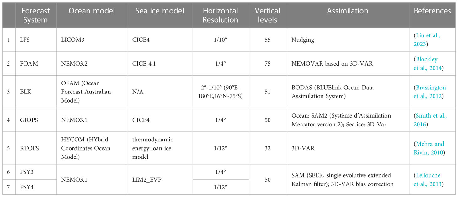
Table 1 Basic information of the forecast systems analyzed.

The IVTT provides an abundance of in-situ drifters and Argo profiles observations. In this study, we evaluate the LFS outputs against IVTT datasets using the following approach. First, the forecast results are extracted and interpolated onto the observation sites from the nearest grid points. Second, metrics for SST statistics are computed directly by comparing the forecasts with drifter measurements. For the temperature and salinity profiles statistics, the following processes is employed: both Argo and forecast data are sampled by depth range according to the prescribed 40 vertical levels. Values within each level are averaged to represent the mean value for that level, and then metrics are calculated by comparing the forecast with the Argo values. This methodology is similar to the approach in Ryan et al. (2015), where 50 levels are used, and the median value servers as the representative. However, this difference does not impact the overall analysis results. The IVTT framework also offers persisted forecasts and the World Ocean Atlas 2001 (WOA2001) as climatological reference, which can be used to assess forecast skills through the Persistence Skill Score (PSS) and Climatological Skill Score (CSS), respectively. The definition of PSS and CSS follows those provided by Ryan et al. (2015).

3 Results

3.1 Sea surface temperature

The sea surface temperatures (SST) from the forecast systems are compared to the in-situ drifter observations, as shown in Figure 1. LFS exhibits a warm bias in the global mean SST, which amounts to approximately 0.05°C at the first forecast lead day (day 1). The median warm bias is comparable to those observed in other systems (Figure 2A). This warm bias increases with the forecast time, reaching around 0.1°C on the sixth day (day 6). Such bias may be related to the slightly overestimated incoming solar radiation in the atmospheric forcing, which contributes to the warm bias accumulated during the forecast processes. Despite the warm bias, LFS demonstrates a relatively small SST RMSE within the forecast period among all the forecast systems. The RMSE value is about 0.53°C on day one, increasing to about 0.63°C on day 6 (Figure 2B). The growth rate of RMSE with the forecast time in LFS is similar to those observed in PSY3/4 and GIOPS.

FIGURE 2

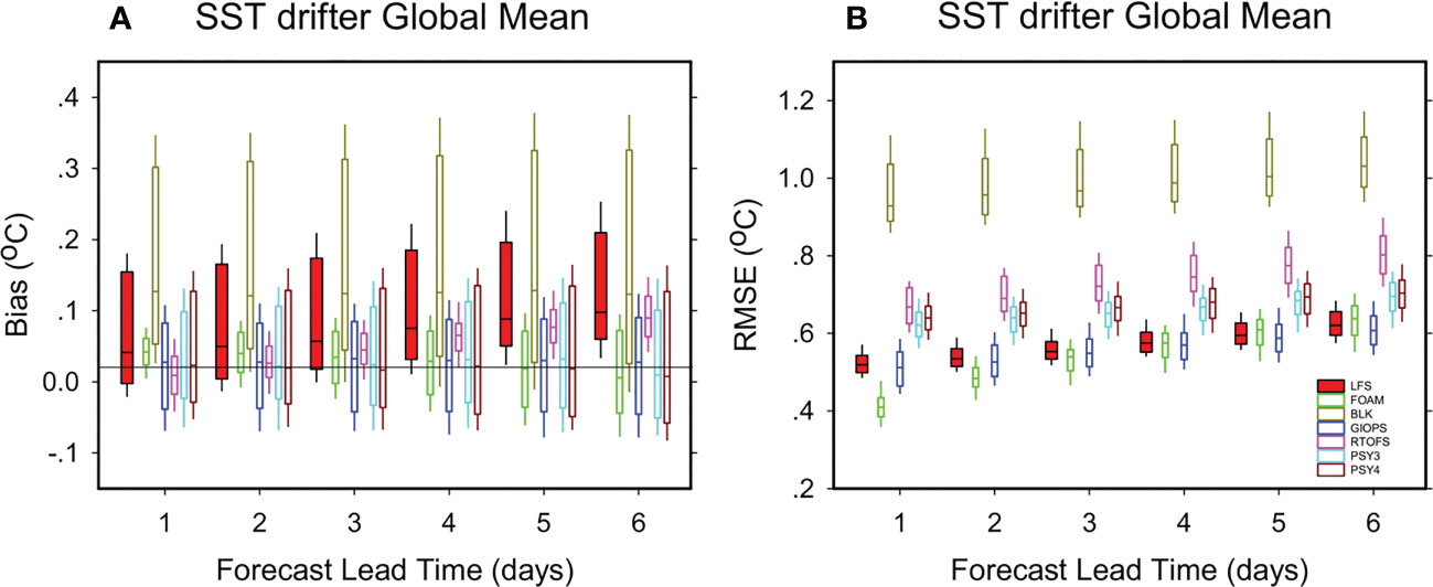
Figure 2 Bias and RMSE of the forecast SST against the in-situ drifters as a function of lead time. (A) Bias; (B) RMSE. The boxes show the range of the 95^th percentile.

Figure 3 shows the SST bias and RMSE at 1 day lead over the forecast period. All the forecast systems show similar behavior, with relatively small SST biases in summer than increase during late autumn and winter. LFS displays a bias in the middle of the forecast systems in summer, while the bias grows larger in autumn and winter (Figure 3A). It is important to note that since PSY4 analysis data serves as the nudging observations for LFS, the SST RMSE is expected to be similar to PSY4 at day 1. However, the RMSE in LFS is consistently smaller than PSY4 over the forecast period (Figure 3B), partially attributable to the nudging time scale employed in ExpA. Additionally, the differences in external atmospheric forcing and the configurations of the systems may contribute to this feature as well.

FIGURE 3

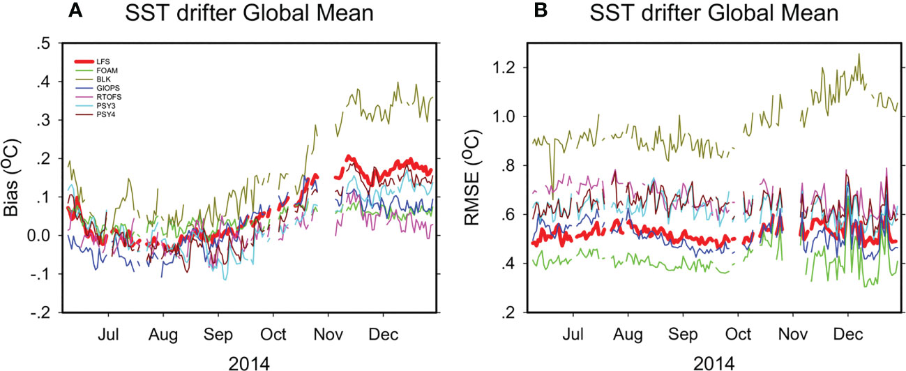
Figure 3 The time series of forecast SST at day 1 for (A) bias; (B) RMSE.

The anomaly correlation coefficient (AC) generally represents the predictability of the forecast system, which is commonly used in short-time and seasonal climate predictions. The anomaly correlation coefficient of SST in LFS is about 0.79 on day 1 and 0.72 on day 6, remaining above 0.6 throughout the forecast period as most of the ocean forecast systems (Figure 4A). Over the entire forecast period, the anomaly correlation coefficient of SST in LFS ranges between 0.6 and 0.8. The AC variation in winter (November-December) is more significant than in other seasons (June-October), a feature also observed in other forecast systems (Figure 4B).

FIGURE 4

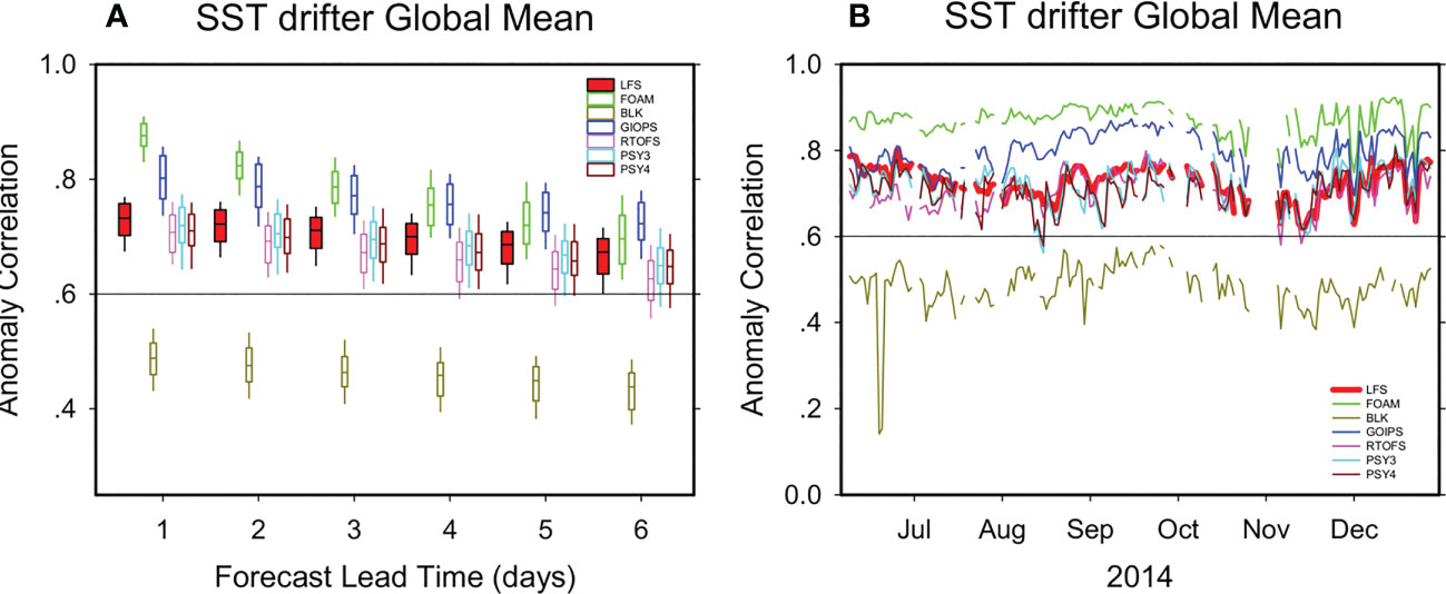
Figure 4 (A) The anomaly correlation coefficient and (B) the time series of anomaly correlation at day 1 for all the forecast systems.

IVTT Class4 provides the two reference datasets, climatological and persisted forecast, from which the CSS and PSS can be obtained by comparing against the WOA2001 climatology and the persisted one-day forecast, respectively. For all forecast systems, the CSS is positive and decreases as the forecast time increases, indicating positive skill against the climatology (Figure 5A). The CSS of SST in LFS is in the middle of all forecast systems, similar to the performance of the anomaly correlation coefficient (Figure 4A), which agrees with the positive relationship between a robust anomaly correlation coefficient and strong positive skill against climatology. For PSS, most forecast systems show an initial weak negative value and a slightly positive trend as the forecast time increases, implying that a 1-day lead forecast is considerable more accurate and skillful than other lead times. The PSS of SST in LFS remains positive over the forecast period (Figure 5B); however, a weak negative trend appears as forecast time increases, potentially related to the simple nudging method used to generate the initial state for the LFS forecast. The SST information is gradually diminishing as the forecast is integrated over six days.

FIGURE 5

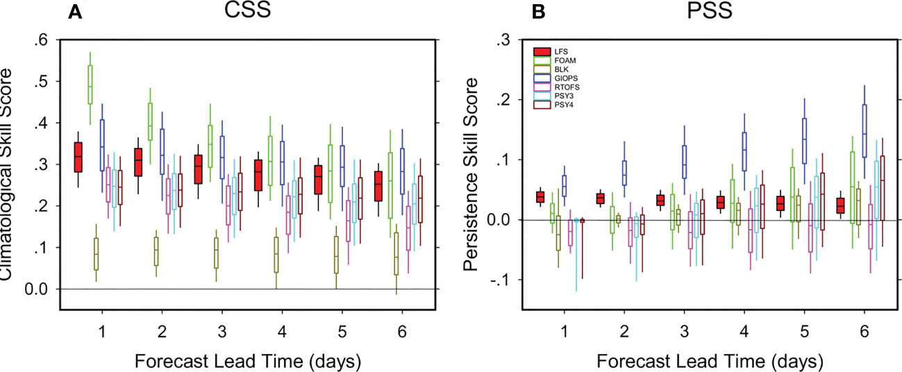
Figure 5 (A) The climatological skill score (CSS) and (B) persistent skill scores (PSS) of the forecast SST against the SST measurements from the drifters as a function of lead time.

3.2 Sea level anomaly

The sea level anomaly (SLA) of LFS is computed by subtracting the SSH climatology from ExpA from the forecast data. Figure 6 shows the bias and RMSE of SLA for all the forecast systems. Most forecast systems have a negative SLA bias, with LFS having a median value of approximately −0.06 m. The bias does not exhibit significant changes during the forecast period, consistent with the behavior of other forecast systems (Figure 6A). The SLA RMSE of LFS is around 0.10 m, falling within the range of other forecast systems (0.07–0.15m, Figure 6B). Similar to SST, both SLA RMSE and Bias increase slightly in the winter season (Figure not shown).

FIGURE 6

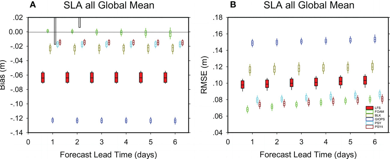
Figure 6 Bias and RMSE of the forecast SLA against the satellite altimeters as a function of lead time. (A) Bias; (B) RMSE. The boxes show the range of the 95^th percentile.

There are several possible explanations for the relatively large negative SLA biases in LFS. Firstly, we do not apply nudging method to the SLA, meaning that the constrain of observation is absent in the initial state from ExpA. Secondly, the Exp has only 7 months of simulation, and although the mean SSH pattern closely resemble that of Mercator PSY4, it does not necessarily imply that the climatology is sufficiently accurate or that the SLA is directly comparable to satellite data.

3.3 Temperature and salinity profiles

The global Argo network can provide more than 3000 floats in the world. Due to the operational procedure for Argo floats, the daily number of available profiles in IVTT is approximately 300. These daily profiles are subsequently used to evaluate the forecast results for all the systems. Similar to SST, a warm bias is present in the sub-surface temperature in LFS. Despite the warm bias, the RMSE of the temperature profile in LFS is the smallest among the forecast systems throughout the entire forecast period. The median RMSE value is about 0.57°C on day 1 and 0.66°C on day 6 (Figure 7A). The median RMSE of the salinity profile is between 0.12and 0.13 PSU (Figure 7B). Since the sub-surface ocean evolved slower than the surface, the bias and RMSE show only a slightly positive trend over the forecast period. It is not surprising that the value and trend are similar to the PSY4 since the temperature and salinity from the PSY4 analysis are nudged to the initial state for the LFS forecast.

FIGURE 7

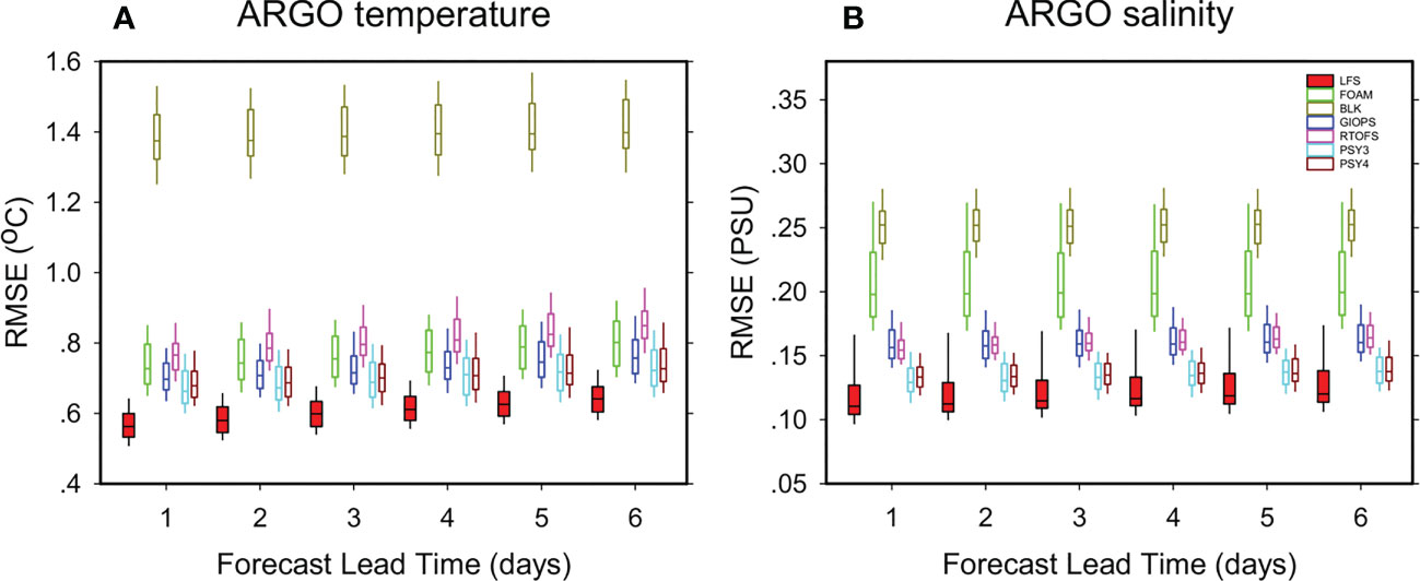
Figure 7 The RMSE of the forecast (A) temperature and (B) salinity against Argo measurements. The boxes show the range of 95th percentile.

Regarding the detailed vertical distribution, all the forecast systems display the most substantial sub-surface temperature errors at the depth of approximately 100 meters (Figure 8A). These errors may be attribute to the strong temperature gradient in the thermocline, which is challenging to simulate in the ocean models. A significant discrepancy exists in the salinity among the forecast systems, particularly in the upper ocean (Figure 8B). LFS has a negative bias of about -0.03 PSU in the upper 50 m. LFS demonstrates a relatively better forecast of the temperature and salinity profiles, as shown in Figure 7, and the RMSE is smaller than most forecast systems.

FIGURE 8

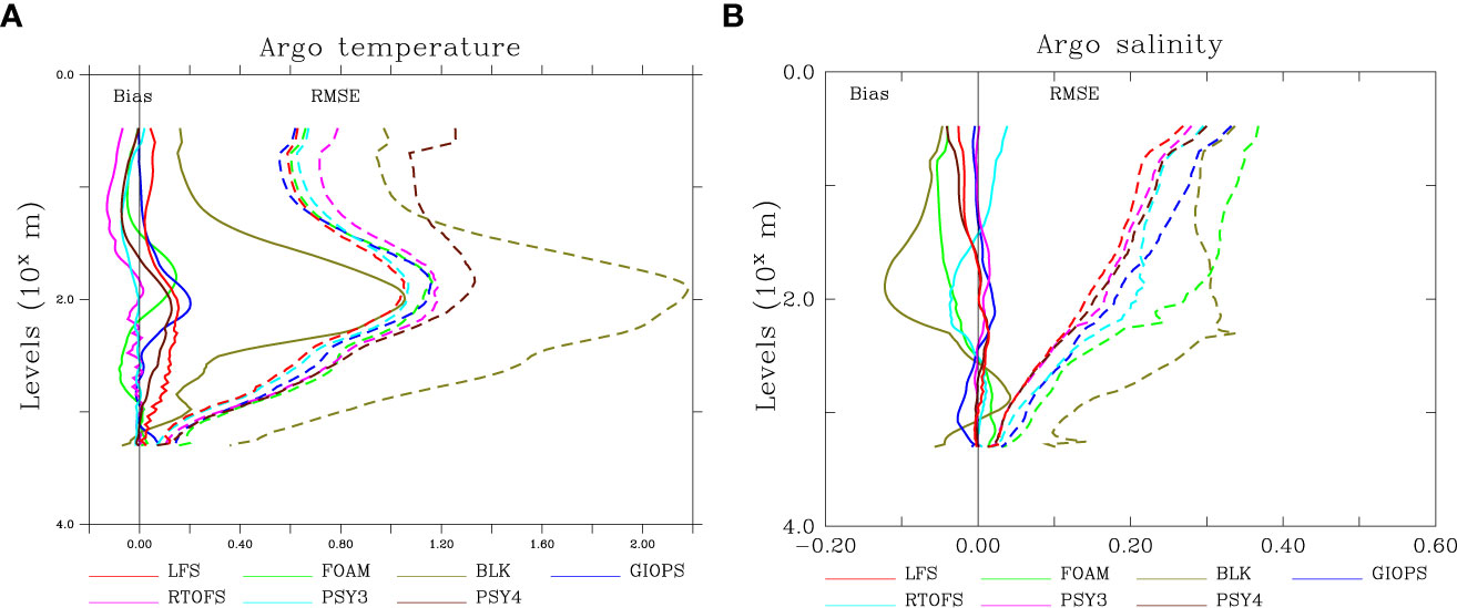
Figure 8 The bias and RMSE as a function of depth for the (A) temperature and (B) salinity on day 1. The vertical axis is logarithmic.

3.4 Regional features

The regional features are assessed based on the ocean basin division in IVTT Class 4 (Table 2). The global ocean is divided into eight basins with overlapping regions. Then the 1 day lead forecast RMSE of SST, SLA, temperature, and salinity are shown as a function of ocean basins in Figure 9, respectively. Generally, most forecast systems exhibit relatively smaller SST RMSE in the tropical regions of the Atlantic and Pacific but larger values in the North Pacific, North Atlantic, and South Atlantic. The model spread is substantial in the subtropical regions, suggesting model differences in representing the mesoscale processes that influence the forecast results. The performance of LFS is broadly consistent with other systems, showing smaller RMSE in the tropical ocean and larger RMSE in the subtropics for SST (Figure 9A). The situation for SLA mirrors that of SST. The regional accuracy in LFS is also the best in the tropical Atlantic but is poor in the South Atlantic. The North Atlantic and Pacific also have regions with considerable biases (Figure 9B). Although the western boundary currents and mesoscale eddies are reproduced in LFS, the strength and locations are not well matched with the observations, resulting in larger RMSE in subtropical regions.

TABLE 2

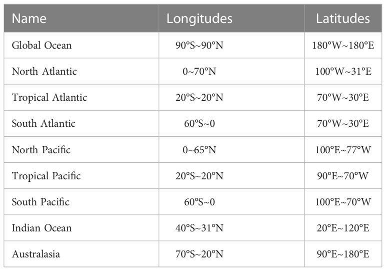
Table 2 IVTT Class 4 ocean basins.

FIGURE 9

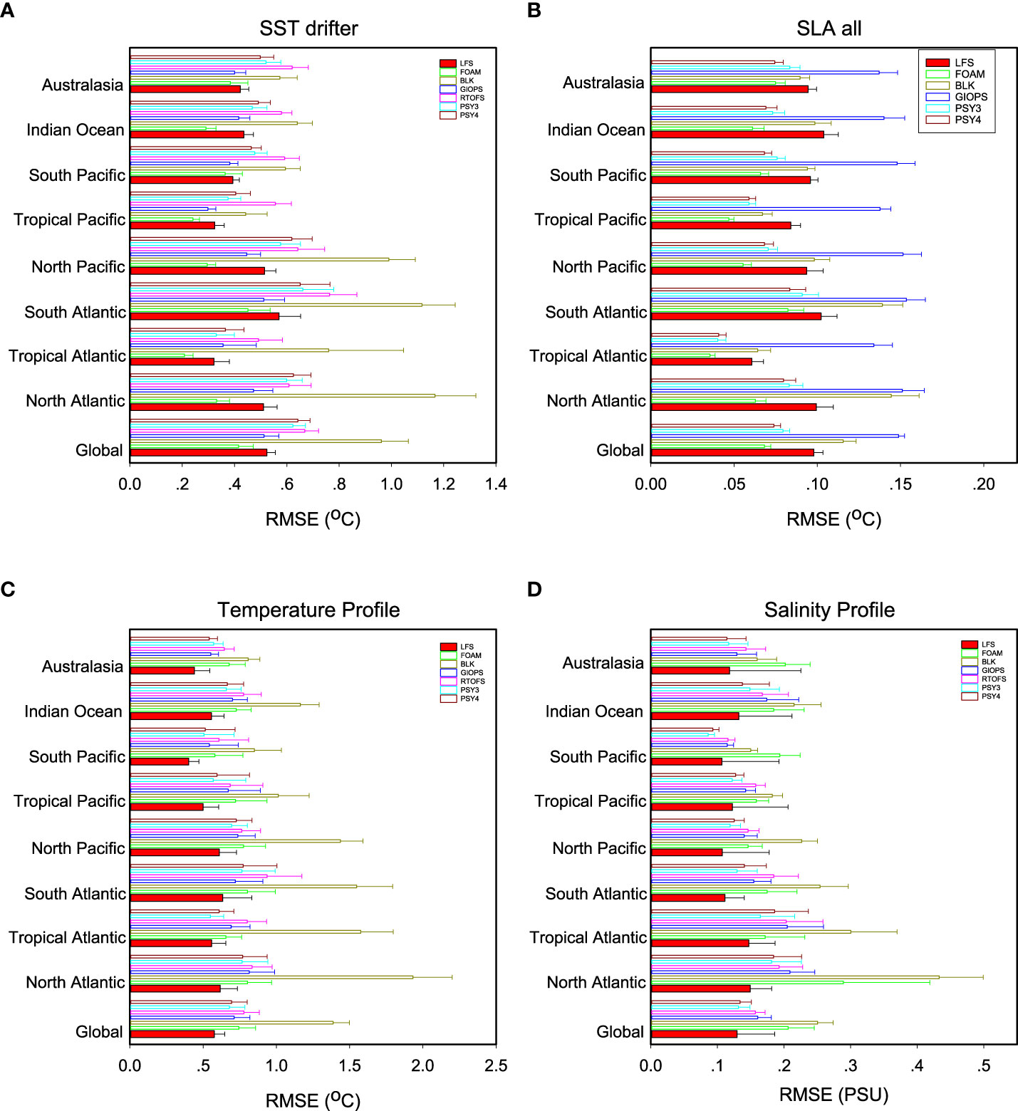
Figure 9 Regional RMSE at leading 1-day for (A) SST against the in-situ drifters, (B) SLA, (C) temperature and (D) salinity against Argo profiles.

The RMSE of temperature and salinity, when compared against Argo profiles, shows a different pattern than that of SST. No significant differences can be identified among ocean basins, which may be attributed to the considerable RMSE in the upper ocean surrounding the thermocline in the tropics. LFS is the most accurate system in forecasting the temperature and salinity in nearly all ocean basins (Figures 9C, D), surpassing even the PSY4 system, whose analysis data were used for LFS initial condition by nudging methods. LFS performs better in the open ocean, such as in the south Pacific, than in other basins for both temperature and salinity. The subtropical ocean basins remain a challenge for accurate forecasting.

4 Conclusions and discussions

Within the evaluation framework of IVTT, the LICOM Forecast System (LFS) forecast results are assessed and compared to other marine forecast systems in this study. LFS demonstrates a reasonably good performance in the short-term marine environment forecasting. The global RMSE of SST, when compared against the drifter observations, ranges from 0.53-0.63°C in the forecast period, ranking in the middle of all the forecast systems. Regional decomposition reveals that LFS has better forecast skills in tropical regions, while exhibiting relatively large biases in the subtropics where the eddies are more active. The temperature and salinity profiles in LFS tend to outperform those in other systems. The RMSE of temperature in LFS against the Argo profile in the upper 2000 m ranges from 0.57-0.66°C in the forecast period, whereas the RMSE of salinity in LFS ranges between 0.12 and 0.13 psu. Across all forecast systems, the maximum RMSE of temperature occurs at a depth of around 100 meters, indicating challenges in reproducing the thermocline variations. The largest RMSE of salinity is at the surface, influenced by water mass and heat fluxes exchanges between the atmosphere and the ocean.

In this iteration of LFS, the initial state was derived by nudging the temperature and salinity of the PSY4, with no additional observational data assimilated into the LFS. The nudging method appears to be a cost-effective approach for obtaining the necessary initial state. In this study, the nudging time scale is set at 5 days for the upper ocean and 20 days for the deep sea. This configuration effectively retains the impacts of mesoscale eddies in the upper ocean while eliminate the weather scale bias, thus favoring the slow growth of biases in the forecasting. Despite the relatively satisfactory performance in capturing the large-scale features, LFS exhibits some defects in predicting the global sea level height anomaly (SLA). The poor performance of SLA may be related to the systematic bias in the climatology, which may be related to unpredictable instabilities. The absence of sea surface height observational data may also have contribution, because nudging the SLA may result in the inconsistency in temperature and salinity that lead to the model’s shock, as discussed by Liu et al. (2023). To address these limitations, it is crucial to develop a coordinated assimilation system for LFS, enabling the incorporation of more observational data to provide a more accurate initial condition for the marine forecast.

Data availability statement

The raw data supporting the conclusions of this article will be made available by the authors, without undue reservation.

Author contributions

WZ, PL, and HL contributed to the development of LFS and the conception of this study. WZ performed the forecast and wrote the first draft of the manuscript. PL and HL wrote sections of the manuscript. YL and JM organized and processed the data. HM and JL performed the statistical analysis. All authors contributed to the article and approved the submitted version.

Funding

This study is supported by the National Key R&D Program for Developing Basic Sciences (2022YFC3104802, 2020YFA0608902), the Special Funds for Creative Research (2022C61540), and the National Natural Science Foundation of China (Grants 41931183, 41976026, 41931182, U2242214).

Acknowledgments

The authors acknowledge the technical support from the National Key Scientific and Technological Infrastructure project “Earth System Science Numerical Simulator Facility” (EarthLab).

Conflict of interest

The authors declare that the research was conducted without any commercial or financial relationships that could be construed as a potential conflict of interest.

Publisher’s note

All claims expressed in this article are solely those of the authors and do not necessarily represent those of their affiliated organizations, or those of the publisher, the editors and the reviewers. Any product that may be evaluated in this article, or claim that may be made by its manufacturer, is not guaranteed or endorsed by the publisher.

References

Blockley E. W., Martin M. J., McLaren A. J., Ryan A. G., Waters J., Lea D. J., et al. (2014). Recent development of the met office operational ocean forecasting system: an overview and assessment of the new global foam forecasts. Geosci. Model. Dev. 7 (6), 2613–2638. doi: 10.5194/gmd-7-2613-2014

CrossRef Full Text | Google Scholar

Brassington G. B., Freeman J., Huang T., Pugh P. R., Sandery A., Taylor A., et al. (2012). “Ocean model analisys and prediction system: version 2,” in CAWCR Technical Report No. 052, The Centre for Weather and Climate Research.

Google Scholar

Ferreira D., Marshall J., Heimbach P. (2005). Estimating eddy stresses by fitting dynamics to observations using a residual-mean ocean circulation model and its adjoint. J. Phys. Oceanogr. 35, 1891–1910. doi: 10.1175/JPO2785.1

CrossRef Full Text | Google Scholar

Gurvan M., Bourdallé-Badie R., Pierre-Antoine B., Clement B., Bruciaferri D., Calvert D., et al. (2017). Nemo ocean engine: Notes du Pôle de modélisation de l'Institut Pierre-Simon Laplace (IPSL). (27). doi: 10.5281/zenodo.1472492

CrossRef Full Text | Google Scholar

Hunke E. C., Lipscomb W. H. (2010). “Cice: the Los alamos Sea ice model,” in Documentation and software users manual, version 4.1 (La-Cc-06-012), vol. 2010. (Los Alamos: T-3 Fluid Dynamics Group, Los Alamos National Laboratory).

Google Scholar

Large W. G., Yeager S. (2004). “Diurnal to decadal global forcing for ocean and Sea-ice models: the data sets and flux climatologies,” in NCAR Technical Note. NCAR/TN-460+STR. doi: 10.5065/D6KK98Q6

CrossRef Full Text | Google Scholar

Lellouche J. M., Greiner E., Le Galloudec O., Garric G., Regnier C., Drevillon M., et al. (2018). Recent updates to the Copernicus marine service global ocean monitoring and forecasting real-time 112° high-resolution system. Ocean Sci. 14 (5), 1093–1126. doi: 10.5194/os-14-1093-2018

CrossRef Full Text | Google Scholar

Lellouche J. M., Le Galloudec O., Drévillon M., Régnier C., Greiner E., Garric G., et al. (2013). Evaluation of global monitoring and forecasting systems at Mercator océan. Ocean Sci. 9 (1), 57–81. doi: 10.5194/os-9-57-2013

CrossRef Full Text | Google Scholar

Li Y., Liu H., Ding M., Lin P., Yu Z., Yu Y., et al. (2020). Eddy-resolving simulation of cas-Licom3 for phase 2 of the ocean model intercomparison project. Adv. Atmospheric Sci. 37 (10), 1067–1080. doi: 10.1007/s00376-020-0057-z

CrossRef Full Text | Google Scholar

Lin P. F., Liu H. L., Xue W., Li H. M., Jiang J. R., Song M. R., et al. (2016). A coupled experiment with Licom2 as the ocean component of Cesm1. J. Meteorol. Res. 30 (1), 76–92. doi: 10.1007/s13351-015-5045-3

CrossRef Full Text | Google Scholar

Lin P. F., Yu Z. P., Liu H. L., Yu Y. Q., Li Y. W., Jiang J. R., et al. (2020). Licom model datasets for the Cmip6 ocean model intercomparison project. Adv. Atmos. Sci. 37 (3), 239–249. doi: 10.1007/s00376-019-9208-5

CrossRef Full Text | Google Scholar

Liu H. L., Lin P. F., Zheng W. P., Luan Y. H., Ma J. F., Ding M. R., et al. (2021). A global eddy-resolving ocean forecast system in China – licom forecast system (Lfs). J. Operational Oceanogr. 16 (1), 15–27. doi: 10.1080/1755876X.2021.1902680

CrossRef Full Text | Google Scholar

Mehra A., Rivin I. (2010). A real time ocean forecast system for the north Atlantic ocean. Terr. Atmos. Ocean. Sci. 21, 211–228. doi: 10.3319/TAO.2009.04.16.01(IWNOP)

CrossRef Full Text | Google Scholar

Murray R. J. (1996). Explicit generation of orthogonal grids for ocean models. J. Comput. Phys. 126 (2), 251–273. doi: 10.1006/jcph.1996.0136

CrossRef Full Text | Google Scholar

Qiao F., Wang G., Khokiattiwong S., Akhir M., Zhu W., Xiao B. (2019). China Published ocean forecasting system for the 21st-century maritime silk road on December 10, 2018. Acta Oceanol. Sin. 38, 1–3. doi: 10.1007/s13131-019-1365-y

CrossRef Full Text | Google Scholar

Ryan A. G., Regnier C., Divakaran P., Spindler T., Mehra A., Smith G. C., et al. (2015). Godae oceanview class 4 forecast verification framework: global ocean inter-comparison. J. Operational Oceanogr. 8 (sup1), s98–s111. doi: 10.1080/1755876X.2015.1022330

CrossRef Full Text | Google Scholar

Schiller A., Mourre B., Drillet Y., Brassington G. (2008). “An overview of operational oceanography,” in New Frontiers in Operational Oceanography. Eds. Chassignet E., Pascual A., Tintoré J., Verron J., 1–26. doi: 10.17125/gov2018.ch01

CrossRef Full Text | Google Scholar

Smith G. C., Roy François, Reszka M., Colan D. S., He Z., Deacu D., et al. (2016). Sea Ice forecast verification in the Canadian global ice ocean prediction system. Q. J. R. Meteorol. Soc. 142 (695), 659–671. doi: 10.1002/qj.2555

CrossRef Full Text | Google Scholar

St. Laurent L. C., Simmons H. L., Jayne S. R. (2002). Estimating tidally driven mixing in the deep ocean. https://doi.org/10.1029/2002GL015633. Geophysical Res. Lett. 29 (23), 21–1-21-4. doi: 10.1029/2002GL015633

CrossRef Full Text | Google Scholar

Tonani M., Balmaseda M., Bertino L., Blockley Ed, Brassington G., Davidson F., et al. (2015). Status and future of global and regional ocean prediction systems. J. Operational Oceanogr. 8 (sup2), s201–ss20. doi: 10.1080/1755876X.2015.1049892

CrossRef Full Text | Google Scholar

Yu Y. Q., Tang S. L., Liu H. L., Lin P. F., Li X. L. (2018). Development and evaluation of the dynamic framework of an ocean general circulation model with arbitrary orthogonal curvilinear coordinate, [In Chinese]. Chin. J. Atmospheric Sci. 42 (4), 877–889. doi: 10.3878/j.issn.1006-9895.1805.17284

CrossRef Full Text | Google Scholar

Yu Z. P., Liu H. L., Lin P. F. (2017). A numerical study of the influence of tidal mixing on Atlantic meridional overturning circulation (Amoc) simulation, [In Chinese]. Chin. J. Atmospheric Sci. 41 (5), 1087–1100. doi: 10.3878/j.issn.1006-9895.1805.17284

CrossRef Full Text | Google Scholar