Hydrodynamic constraint loads estimation on connectors of column-pontoon type very large floating structure (CP-VLFS) under wave stimulation

1 Introduction

The development and application of ocean resources has gradually progressed from the coast to the deep sea (Rayner et al., 2019; Liu and Molina, 2021). Under this background, researches on very large floating structures (VLFSs) have become increasingly significant (Lamas-Pardo et al., 2015; Xiao et al., 2016; Singla et al., 2018; Wei et al., 2018; Yang et al., 2019). VLFSs are the ocean floating structures whose dimensions are measured in kilometers, which can be used as the multi-use floating island (Flikkema and Waals, 2019; Drummen and Olbert, 2021), the platform of offshore wind turbines (Xu et al., 2022), as well as the modular floating terminal (Souravlias et al., 2020), etc. Especially, the column-pontoon type very large floating structure (CP-VLFS) is generally regarded as a significant carrier for human beings to explore ocean resources in deep and faraway sea areas due to their superior hydrodynamic behaviors and their suitability for complex and rough marine environments. The CP-VLFS cannot be produced as a whole due to their very large scale, which are typically fabricated structures and require the connectors with specially designed to combine the multiple CP-VLFS modules together (Wang and Tay, 2011). These connectors must be the weaknesses for the entire structure of CP-VLFS, and very large hydrodynamic constraint loads will occur on connectors under the external marine environment forces, especially, the most unfavorable forces on CP-VLFS modules (Lamas-Pardo et al., 2015). Therefore, it is critical to develop a rapid, high-efficiency and reasonable method to estimate the hydrodynamic constraint loads of connectors on CP-VLFSs under the complicated external excitation forces.

The different connection types (rigid or flexible) between the two adjacent VLFSs modules can directly determine the constraint loads of connectors (Gao et al., 2011). Simplified mathematical and mechanical models of the CP-VLFSs’ modules and connectors have been classified into four aspects according to the rigidity or flexibility of the modules and connectors (Wu et al., 2017), including the rigid-module with flexible-connector (RMFC) model, the rigid-module with rigid-connector (RMRC) model, the flexible-module with rigid-connector (FMRC) model, and the flexible-module with flexible-connector (FMFC) model. Particularly, the RMFC model is adopted the most widely and indicates that the CP-VLFS modules’ stiffness is infinitely greater than those of their connectors (Wu et al., 2017). This means that the CP-VLFSs’ modules cannot appear to deform, but only exhibiting the translation and rotation when the structures are stimulated via marine environmental loads. Meanwhile, the connectors are flexible and exhibit relative deformation, which generates very large constraint loads.

General mainstream technique for determining the hydrodynamic coefficient and environmental fluid force of marine structures, especially the floating structures, is almost based on the theories of PFT (Lian et al., 2020; Qiao et al., 2020), and some business software, such as the SESAM of DNV, WAMIT, AQWA of ANSYS, etc., on the basis of the PFT are used to investigate the frequency- and/or time-domain hydrodynamic parameters and fluid forces on floating bodies.

Kim et al. (2014) proposed a hydroelastic design contour practically used for the preliminary design of pontoon-type rectangular VLFSs, and the PFT was used to model the fluid forces on VLFS. Wei et al. (2017) proposed a numerical method for predicting the hydroelastic responses of VLFS by using the three-dimensional PFT and finite element method, and the influences of inhomogeneous seabed and wave field conditions were considered during this method. In addition, Wei et al. (2018) developed a time-domain estimating method for investigating the hydroelastic responses of a freely VLFSs under inhomogeneous regular and irregular waves, and the method of PFT was utilized to determine the hydrodynamic coefficients and wave excitation forces acting on VLFS. Wu et al. (2017) developed a simplified algorithm for assessing the hydrodynamic performances of a three-module semi-submersible type VLFS, as well as the hydrodynamic responses of connectors for VLFS at rough sea states were analyzed (Wu et al., 2016a). On the basis of the simplified method and the hydrodynamic response results of VLFS, the optimal stiffnesses of connectors for this VLFS were determined (Wu et al., 2018). Ding et al. (2017) established a direct coupled method based on Boussinesq equations and RANKINE source method to evaluate the hydroelastic responses of a single module VLFS near islands and reefs. Next, Ding et al. (2019) developed a simplified method and a software of THAFTS-IHIW to evaluate the hydroelastic responses of an eight-module VLFS under the inhomogeneous waves in the Typhoon of Kalmaegi. During the numerical calculation process, the PFT was used to confirm the wave excitation forces of VLFS. Subsequently, Ding et al. (2020a) utilized the experimental and numerical methods to investigate the hydroelastic responses of an eight-module VLFS deployed in shallow water and near a typical island. The module motions and connector loads of the VLFS were analyzed in detail. During the numerical method, the PFT was adopted and combined with classical hydroelasticity theory to assess the dynamic responses of VLFS. Moreover, Ding et al. (2020b) investigated the loads of flexible connectors installed in a three-module VLFS floated in the shallow water areas based on the methods of physical experiment and numerical computation. The three-dimensional hydroelasticity theory based on PFT and RMFC model were used to build a simplified analysis procedure for estimating the connector loads of VLFS, and the influences of uneven seabed were considered. Ding R. et al. (2020) carried out a physical experiment to investigate characteristic evolution for a chain-type floating system with increase of module numbers. The connector loads of the experimental prototypes were estimated on the basis of RMFC model and experimental measurements.

Qi et al. (2018) provided a fatigue estimation for a VLFS by using a spectral-based fracture mechanics approach united hydrodynamic response analysis based on PFT (ANSYS AQWA), spectral stress intensity factor calculation, load spectrum, and fatigue crack propagation model. Shi Q. J. et al. (2018) focused on the design of stiffness of flexible-base hinged connector stiffness for a three-modular VLFS. During this process, the orthogonal experimental method was adopted to consider the relationship between the connectors’ stiffness combination and VLFS module responses, and the hydrodynamic forces on VLFS were estimated by using the PFT. Ren et al. (2019) investigated the influence of outermost connector types on time-domain hydrodynamic responses of a modular multi-purpose floating structure system with seven modules by using the numerical method. The linear PFT was used to estimate the wave force on modular multi-purpose floating structure during the numerical computation. Zhao et al. (2019) proposed a genetic-algorithm-based routine procedure and subsequently developed a method to properly determine anisotropic stiffness of connectors for multi-modular floating systems under various wave conditions. During the numerical investigations, the PFT was adopted to analyze the linear wave force on floating structure, and the optimal stiffness configuration for an 8-modular floating system was determined according to this aforementioned method.

On the basis of the aforementioned contents, some useful information can be obtained: PFT still remains the main research approach for studying the hydrodynamic characteristics of VLFSs and their connectors. Although the PFT method has powerful universal applicability, the corresponding theories are relatively complex and would consume plenty of computing time. Generally, increasing the accuracy of estimated results but sacrificing the solving efficiency must consume more computational time to acquire the satisfactory results. Nevertheless, during the preliminary design and scheme comparison stages for CP-VLFS, the hydrodynamic results of CP-VLFSs and their connectors required to be rapidly and high-efficiently determined, but it is unnecessary to ensure the estimation accuracy of the structural hydrodynamic results absolutely consisting with those of the design stage of construction.

For this paper’s investigations, a rapid and high-efficiency estimating method for time-domain hydrodynamic constraint loads of connectors on CP-VLFS considering the RMFC model at high sea states (HSSs) is developed via this paper based on some reasonable assumptions. The Morison theory for floating body is employed to assess the external excitation forces of RIW on CP-VLFS modules, and a series of theoretical formulas for the hydrodynamic constraint loads of connectors are derived on the basis of the geometrical relationships of CP-VLFS modules’ motion. A three-modules model of CP-VLFS at sea state six (SS6) is regarded as a case, and the estimation results via this paper’s high-efficiency method are compared with the results by PFT method and the measurements from a referenced physical model test. Finally, the relative errors among the results by the methods of this paper, PFT, as well as the model test are simultaneously analyzed to elaborate the precision, feasibility and reasonability of this paper’s high-efficiency method.

2 Theoretical analysis

2.1 General concept

The conceptual design scheme for CP-VLFS is exhibited in Figure 1, in which consists of many individual modules connected by connectors. A single CP-VLFS module constituted by three components, including one top platform, eight columns and two pontoons. The designed flexible connector for CP-VLFS is shown in Figure 2 (Ding et al., 2020b).

FIGURE 1

Figure 1 Conceptual design scheme for CP-VLFS.

FIGURE 2

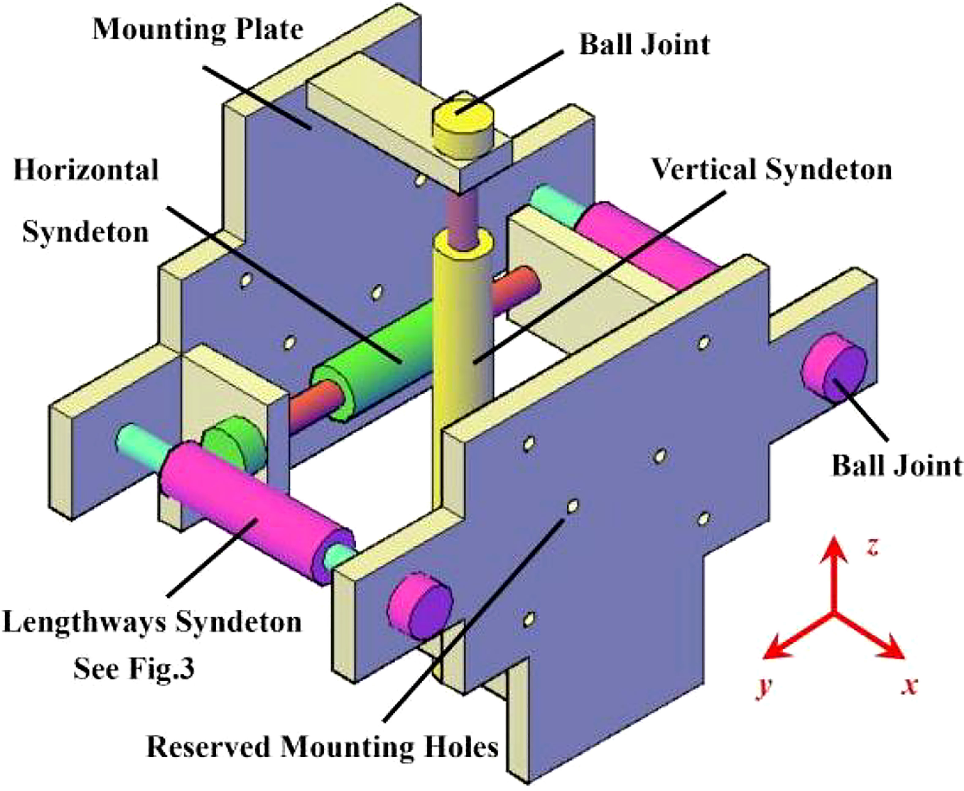
Figure 2 Designed flexible connector of CP-VLFS.

The flexible connector of CP-VLFS has been designed to prevent the linear displacement of CP-VLFS modules’ motion but allow their angular rotation in three translational directions, which can be carried out by using the springs with stiffness placed into a significant device of syndeton. The key components of a single syndeton are as shown in Figure 3, and the design principles, specific functions for various components of a syndeton are explained by Wu et al., 2016b. Figure 2 elaborates the CP-VLFS flexible connectors with the multiple syndetons in x, y, and z directions, which are the important components for CP-VLFS’s flexible connectors.

FIGURE 3

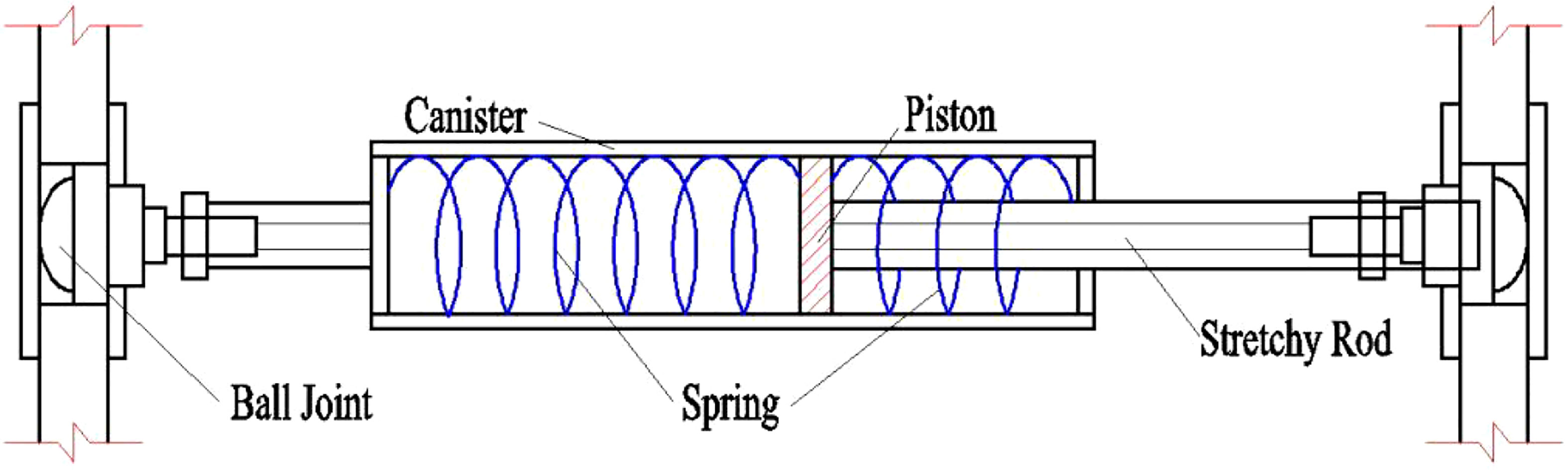
Figure 3 Schematic diagram of the syndeton.

This paper considers the flexible connector of CP-VLFS as a simplified spring model in terms of the calculation model of RMFC, as shown in Figure 4, as well as the k_x, k_y, and k_zare the connectors’ stiffnesses in the directions of x, y, and z, respectively. Therefore, the constraint loads of flexible connectors in the directions of x, y, and z are estimated by Hook’s Law:

FIGURE 4

Figure 4 Simplified spring model of a flexible connector.

$\begin{array}{ll}\{\begin{array}{l}{F}_{cx}^{C_{i,i+1}^m}=k_{x{C}_{i,i+1}^m}\Delta x_{C_{i,i+1}^m}\\ F_{cy}^{C_{i,i+1}^m}=k_{y{C}_{i,i+1}^m}\Delta y_{C_{i,i+1}^m}\\ F_{cz}^{C_{i,i+1}^m}=k_{z{C}_{i,i+1}^m}\Delta z_{C_{i,i+1}^m}\end{array}& (1)\end{array}$

where i means the module i (M_i) of the CP-VLFS; $C_{i,i+1}^m$ represents the connector m among the module i (M_i) and module i+1 (M_i+1), where m=1,2,···j; and j denotes the number of connectors between the two adjacent CP-VLFS modules. The symbols of $k_{x{C}_{i,i+1}^m}$, $k_{y{C}_{i,i+1}^m}$, and $k_{z{C}_{i,i+1}^m}$ are the stiffnesses of $C_{i,i+1}^m$ in the directions of x, y, and z, respectively. Meanwhile, the $\Delta x_{C_{i,i+1}^m}$, $\Delta y_{C_{i,i+1}^m}$, and $\Delta z_{C_{i,i+1}^m}$ denote the relative deformations of $C_{i,i+1}^m$ in the directions of x, y, and z, respectively.

Within Eq. (1), the connectors’ stiffnesses are the known parameters, therefore the key issue for estimating the constraint loads of CP-VLFS’s connectors is determining the connectors’ relative deformations in different directions of x, y, and z. The relative deformations occur on CP-VLFS’s flexible connectors due to the two adjacent modules experience relative motion under the external marine environmental loads. Therefore, the precondition for acquiring the relative deformations of CP-VLFS’s connectors is determining the connectors’ hydrodynamic deformations between the two adjacent modules of CP-VLFS.

To sum up, this paper regards a multi-modules CP-VLFS as a multiple degree-of-freedom (DOF) system of structural dynamics theory. Figure 5 shows the simplified RMFC model for CP-VLFS with modules and connectors.

FIGURE 5

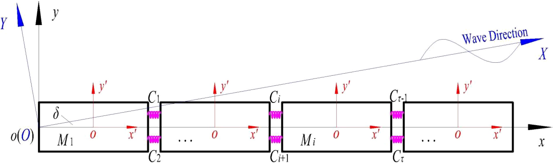
Figure 5 Simplified RMFC model for the module and connectors of CP-VLFS and its coordinate system (oxy plane).

In Figure 5, M_i (i = 1, 2,…) is the module i and C_τ(τ = 1, 2,…) is the connector τ. On the basis of D’Alembert’s principle, the structural dynamic equation (Wang et al., 2022a) for CP-VLFS is written as follows:

$\begin{array}{ll}[M]\left\{\ddot{X}\right\}+[C_f]\left\{\dot{X}\right\}+[K]\left\{X\right\}=\left\{F_w\right\}& (2)\end{array}$

where [M]=[M_s]+[M_f], [M_s] is the mass matrix and [M_f] is the added mass matrix of CP-VLFS. [C_f] is the structural damping coefficient matrix. [K] is the stiffness matrix for floating structure, and [K]=[K_s]+[K_f], where [K_s] is the structural global stiffness matrix. [K_f] is the static resilience coefficient matrix. {F_w} is the external excitation force matrix (vector). $\left\{\ddot{X}\right\}$, $\left\{\dot{X}\right\}$, and {X} are the vectors of acceleration, velocity and motion displacement for the CP-VLFS modules, respectively.

Some reasonable assumptions are proposed to facilitate the following theoretical derivation in this paper:

(1) The CP-VLFS has no navigational velocity;

(2) The mooring or anchoring facilities of CP-VLFS are not considered in this paper tentatively, and the restraint boundary conditions for the CP-VLFS models will be explained in detail while solving the dynamical equations;

(3) Only a random and irregular wave (RIW) force at high sea state is regarded as an external excitation force on CP-VLFS modules;

(4) This paper concentrates on researching a high-efficiency method for estimating the hydrodynamic constraint loads of CP-VLFS connectors under the RIW of HSSs acting on. Hence, the CP-VLFS’s columns and pontoons are both considered as the small-scale components via comparing with the very large wavelengths of HSSs (Stansby et al., 2015; Shi Y. et al., 2018).

On the basis of the aforementioned assumptions, {F_w} in Eq. (2) denotes the external force of RIW. Simultaneously, the wave field of RIW varies with the continuous time, so the major parameters in Eq. (2), which consist of the unknowns X=X(t), hydrodynamic coefficients [M_f]=[M_f(t)], [C_f]=[C_f(t)], [K_s]=[K_s(t)], and [K_f]=[K_f(t)] and the wave excitation force {F_w}={F_w(t)}, all vary with time. Inserting these parameters into Eq. (2) changes the dynamic equation to

$\begin{array}{ll}([M_s]+[M_f(t)])\left\{\ddot{X}(t)\right\}+[C_f(t)]\left\{\dot{X}(t)\right\}+([K_s(t)]+[K_f(t)])\left\{X(t)\right\}=\left\{F_w(t)\right\}& (3)\end{array}$

The hydrodynamic relationship for the whole CP-VLFS is expressed via Eq. (3). To facilitate the following analysis, utilizing the isolation method to acquire a CP-VLFS module’s motion equations:

$\begin{array}{ll}([M_s]+[M_f(t)])\left\{\ddot{X}(t)\right\}+[C_f(t)]\left\{\dot{X}(t)\right\}+[K_f(t)]\left\{X(t)\right\}=\left\{F_w(t)\right\}+\left\{F_c(t)\right\}& (4)\end{array}$

In Eq. (4), the global stiffness matrix of CP-VLFS [K_s]=0 means that the entire structure of CP-VLFS is disconnected from the connectors’ positions. Meanwhile, the connectors’ constraint loads {F_c(t)} are changed from internal forces to external forces, as exhibited in Eq. (4).

Each module of CP-VLFS exhibits hydrodynamic response displacements along the six DOF directions, including the surge, sway, heave, roll, pitch and yaw, under the external marine environmental forces of RIW at HSSs. Therefore, six hydrodynamic equations based on the Eq. (4) can be built to solve the hydrodynamic displacements of CP-VLFS module in these six directions, and the hydrodynamic relative deformations for various connectors of CP-VLFS can be derived on the basis of the CP-VLFS connectors’ hydrodynamic deformations as well as the geometrical relationships among the two adjacent CP-VLFS modules’ motions. The CP-VLFS connectors’ hydrodynamic constraint loads can be ultimately estimated by combining the connectors’ relative deformations with Eq. (1). In sum, the research idea and implementation steps for this paper’s simplified method are as follows:

(1) Solve the hydrodynamic equations of a CP-VLFS single module within Eq. (4) to acquire each module’s motion displacements in six DOF directions;

(2) According to the geometrical relationships before and after the two adjacent CP-VLFS modules’ motions to deduce the deformations and relative deformations of CP-VLFS connectors in directions of x, y, and z;

(3) Utilize the Hook’s Law of Eq. (1) to evaluate the hydrodynamic constraint loads of flexible connectors.

The global coordinate system (GCS) oxyz, the local coordinate system (LCS) ox’y’z’, as well as the wave coordinate system (WCS) OXYZ of the CP-VLFS in the oxy, ox’y’ and OXY planes are defined in Figure 5, where δ is the wave angle. The origins of the GCS (o) and WCS (O) are coincident. The incident direction of RIW defines always parallel with the OX axis in OXYZ, and the WCS can revolve around the point O. Figures 6 and 7 present the LCS ox’y’z’ for CP-VLFS module in the ox’z’, oy’z’ planes and the physical dimensions of a single CP-VLFS module. The wave angles can be varied from 0° to 90° in this paper.

FIGURE 6

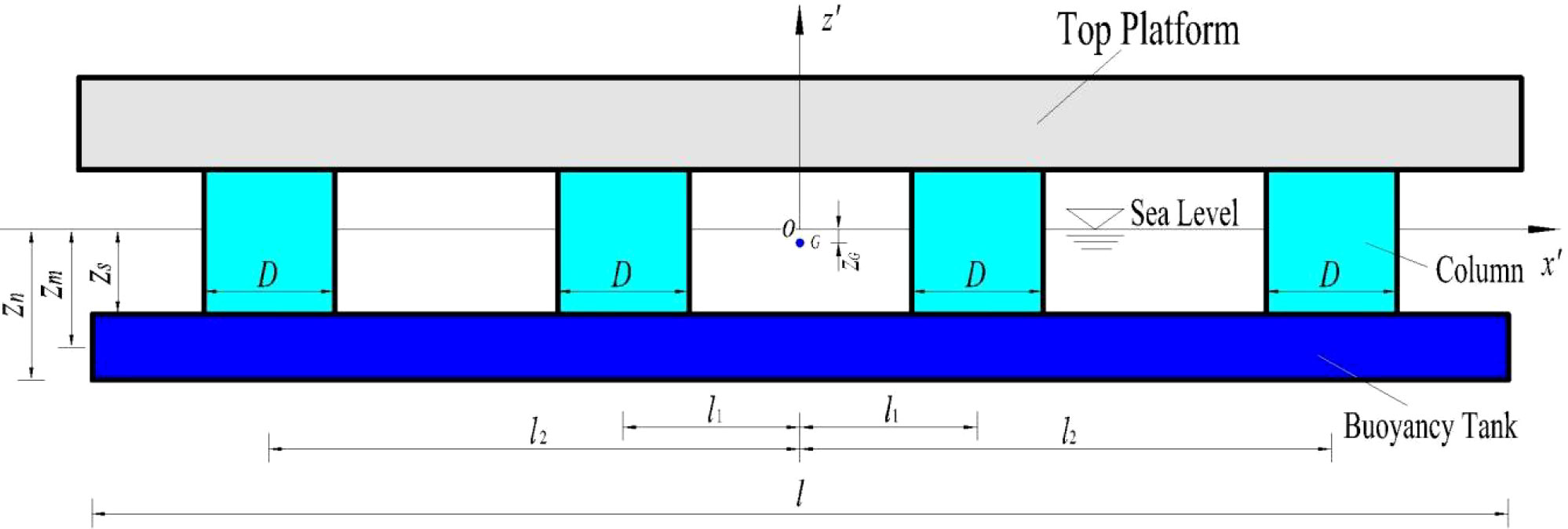
Figure 6 LCS and physical dimensions of a single CP-VLFS module in the ox’z’ plane.

FIGURE 7

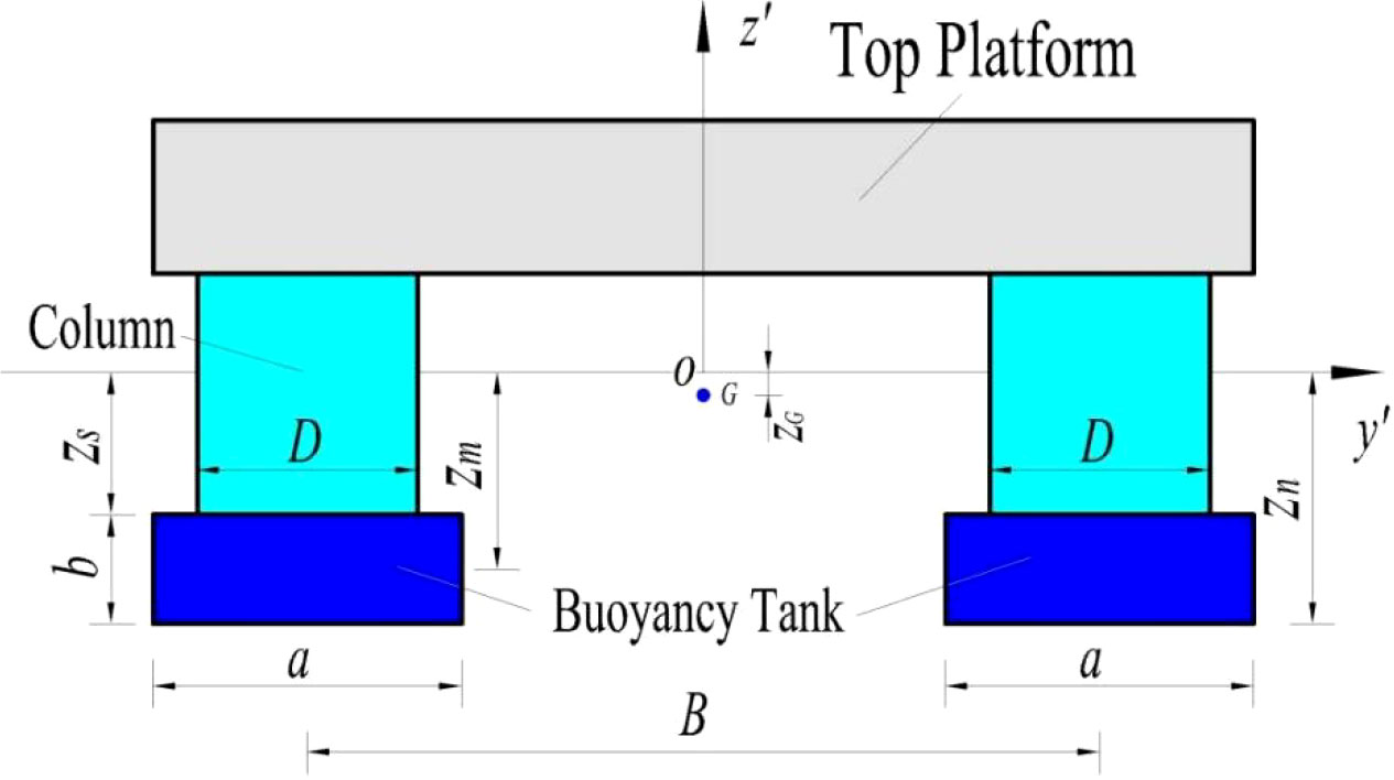
Figure 7 LCS and physical dimensions of a single CP-VLFS module in the oy’z’ plane.

2.2 Hydrodynamic constraint loads for connectors

Figure 8 shows the simplified geometric model for a single module and connectors of CP-VLFS, where the single module is M_i and $C_{i-1,i}^1$, $C_{i-1,i}^2$, $C_{i,i+1}^1$, and $C_{i,i+1}^2$ are the connectors between two adjacent modules. This paper treats $C_{i,i+1}^1$ and $C_{i,i+1}^2$ as instances to derive formulas of the hydrodynamic constraint loads, where $C_{i,i+1}^1$ and $C_{i,i+1}^2$ denote connectors 1 and 2 between M_i and M_i+1. Some of the geometrical parameters for CP-VLFS modules, including R, r, Rr, α, β, and γ, can be determined in Figure 8.

FIGURE 8

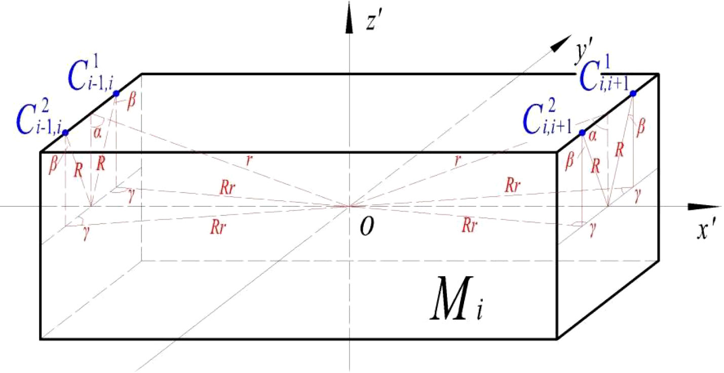
Figure 8 Simplified geometric model for a single CP-VLFS module and connectors.

2.2.1 Deformations and relative deformations of CP-VLFS’s connectors

(1) Due to the translation of CP-VLFS modules

Once the CP-VLFS moves by the external environmental wave forces, the deformations and relative deformations of $C_{i,i+1}^1$and $C_{i,i+1}^2$from the CP-VLFS module’s translation (surge, sway, and heave) in the directions of x’, y’, and z’ are expressed as follows:

(a) x’ direction:

$\begin{array}{ll}\{\begin{array}{l}{x}_{C_{i,i+1}^1}^{Surge(i)}=x_{C_{i,i+1}^2}^{Surge(i)}={\xi }_{x(i)}\\ \Delta x_{C_{i,i+1}^1}^{Surge}=\Delta x_{C_{i,i+1}^2}^{Surge}={\xi }_{x(i+1)}-{\xi }_{x(i)}\end{array}& (5)\end{array}$

(b) y’ direction:

$\begin{array}{ll}\{\begin{array}{l}{y}_{C_{i,i+1}^1}^{Sway(i)}=y_{C_{i,i+1}^2}^{Sway(i)}={\xi }_{y(i)}\\ \Delta y_{C_{i,i+1}^1}^{Sway}=\Delta y_{C_{i,i+1}^2}^{Sway}={\xi }_{y(i+1)}-{\xi }_{y(i)}\end{array}& (6)\end{array}$

(c) z’ direction:

$\begin{array}{ll}\{\begin{array}{l}{z}_{C_{i,i+1}^1}^{Heave(i)}=z_{C_{i,i+1}^2}^{Heave(i)}={\xi }_{z(i)}\\ \Delta z_{C_{i,i+1}^1}^{Heave}=\Delta z_{C_{i,i+1}^2}^{Heave}={\xi }_{z(i+1)}-{\xi }_{z(i)}\end{array}& (7)\end{array}$

where $x_{C_{i,i+1}^1}^{Surge(i)},y_{C_{i,i+1}^1}^{Sway(i)},z_{C_{i,i+1}^1}^{Heave(i)}$ and $x_{C_{i,i+1}^2}^{Surge(i)},y_{C_{i,i+1}^2}^{Sway(i)},z_{C_{i,i+1}^2}^{Heave(i)}$ denote the deformations for $C_{i,i+1}^1$ and $C_{i,i+1}^2$ in the directions of x’, y’, and z’ due to the CP-VLFS module’s translation along the surge, sway, and heave, respectively; $\Delta x_{C_{i,i+1}^1}^{Surge},\Delta y_{C_{i,i+1}^1}^{Sway},\Delta z_{C_{i,i+1}^1}^{Heave}$ and $\Delta x_{C_{i,i+1}^2}^{Surge},\Delta y_{C_{i,i+1}^2}^{Sway},\Delta z_{C_{i,i+1}^2}^{Heave}$ mean the relative deformations for $C_{i,i+1}^1$ and $C_{i,i+1}^2$; as well as ξ_x(i),ξ_y(i),ξ_z(i) and ξ_x(i+1),ξ_y(i+1),ξ_z(i+1) denote the hydrodynamic response displacements for M_i and M_i+1 along the surge, sway, and heave.

(2) Due to the rotation of CP-VLFS modules

Similarly, connectors of CP-VLFS can appear linear deformation due to the two adjacent modules rotation along the directions of roll, pitch, and yaw. The translational deformations for the flexible connectors because of CP-VLFS modules’ rotation are derived by means of the geometrical relationships before and after the CP-VLFS modules’ motions. Some plus or minus symbols are uniformly defined to more advantageously deduce the following contents.

Two standards are stated during the investigations of this paper: firstly, the unknown rotational angles, including θ_x(i), θ_y(i), and θ_z(i) for CP-VLFS modules are negative when M_i is the clockwise rotation around the x’, y’, and z’ axes, as well as their opposites are positive; moreover, the linear deformations of connectors, which are negative when they are the same as the coordinate directions and positive otherwise.

When M_i is rotation along the pitch (as shown in Figure 9), the translational deformations and relative deformations for $C_{i,i+1}^1$ and $C_{i,i+1}^2$ in directions of x’ and z’ are determined in terms of the geometrical relationships of CP-VLFS module before and after rotation:

FIGURE 9

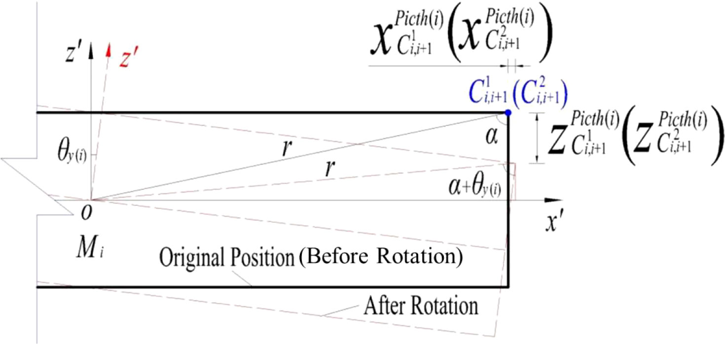
Figure 9 Pitch rotation.

(a) x’ direction:

$\begin{array}{ll}\{\begin{array}{l}{x}_{C_{i,i+1}^1}^{Pitch(i)}=x_{C_{i,i+1}^2}^{Pitch(i)}=-r[\sin (\alpha +{\theta }_{y(i)})-\sin \alpha ]\\ \Delta x_{C_{i,i+1}^1}^{Pitch}=\Delta x_{C_{i,i+1}^2}^{Pitch}=-r[\sin (\alpha +{\theta }_{y(i+1)})-\sin (\alpha +{\theta }_{y(i)})]\end{array}& (8)\end{array}$

(b) z’ direction:

$\begin{array}{ll}\{\begin{array}{l}{z}_{C_{i,i+1}^1}^{Pitch(i)}=z_{C_{i,i+1}^2}^{Pitch(i)}=r[\cos \alpha -\cos (\alpha +{\theta }_{y(i)})]\\ \Delta z_{C_{i,i+1}^1}^{Pitch}=\Delta z_{C_{i,i+1}^2}^{Pitch}=-r[\cos (\alpha +{\theta }_{y(i+1)})-\cos (\alpha +{\theta }_{y(i)})]\end{array}& (9)\end{array}$

When M_i is rotation along the roll (as shown in Figure 10), the translational deformations and relative deformations for $C_{i,i+1}^1$ and $C_{i,i+1}^2$ in directions of y’ and z’ are expressed as:

FIGURE 10

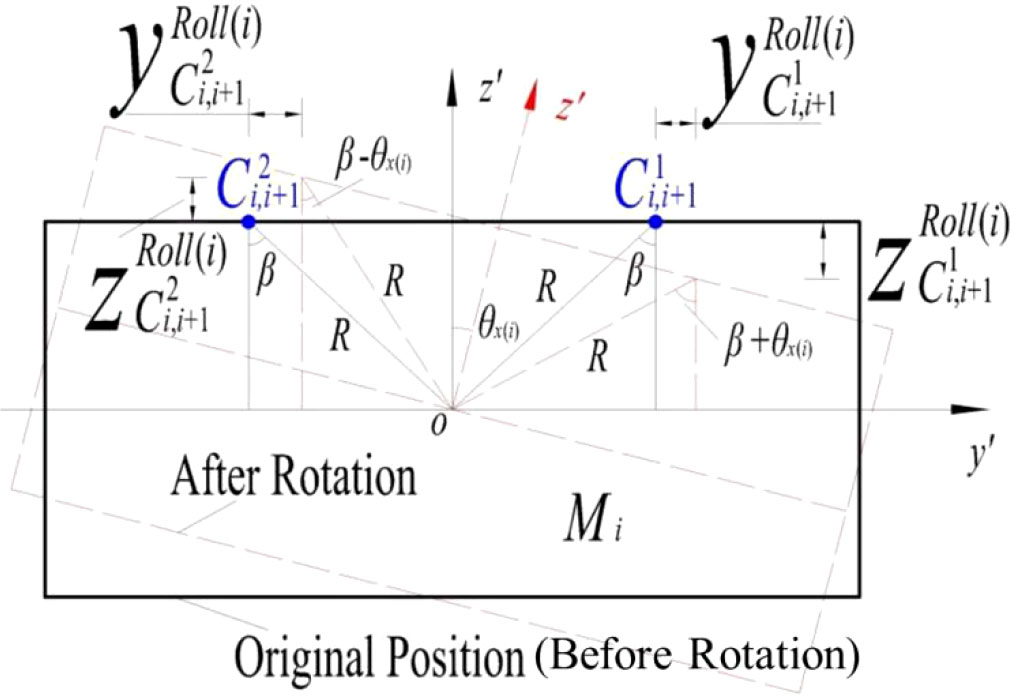
Figure 10 Roll rotation.

(a) y’ direction:

$\begin{array}{ll}\{\begin{array}{l}\begin{array}{cc}{y}_{C_{i,i+1}^1}^{Roll(i)}=-R[\sin (\beta +{\theta }_{x(i)})-\sin \beta ],& y_{C_{i,i+1}^2}^{Roll(i)}=-R[\sin \beta -\sin (\beta -{\theta }_{x(i)})]\end{array}\\ \begin{array}{cc}\Delta y_{C_{i,i+1}^1}^{Roll}=-R[\sin (\beta +{\theta }_{x(i+1)})-\sin (\beta +{\theta }_{x(i)})],& \Delta y_{C_{i,i+1}^2}^{Roll}=R[\sin (\beta -{\theta }_{x(i+1)})-\sin (\beta -{\theta }_{x(i)})]\end{array}\end{array}& (10)\end{array}$

(b) z’ direction:

$\begin{array}{ll}\{\begin{array}{l}\begin{array}{cc}{z}_{C_{i,i+1}^1}^{Roll(i)}=R[\cos \beta -\cos (\beta +{\theta }_{x(i)})],& z_{C_{i,i+1}^2}^{Roll(i)}=-R[\cos (\beta -{\theta }_{x(i)})-\cos \beta ]\end{array}\\ \begin{array}{cc}\Delta z_{C_{i,i+1}^1}^{Roll}=-R[\cos (\beta +{\theta }_{x(i+1)})-\cos (\beta +{\theta }_{x(i)})],& \Delta z_{C_{i,i+1}^2}^{Roll}=-R[\cos (\beta -{\theta }_{x(i+1)})-\cos (\beta -{\theta }_{x(i)})]\end{array}\end{array}& (11)\end{array}$

When Mi is rotation along the yaw (as shown in Figure 11), the translational deformations and relative deformations for $C_{i,i+1}^1$ and $C_{i,i+1}^2$ in directions of x’ and y’ are formed as:

FIGURE 11

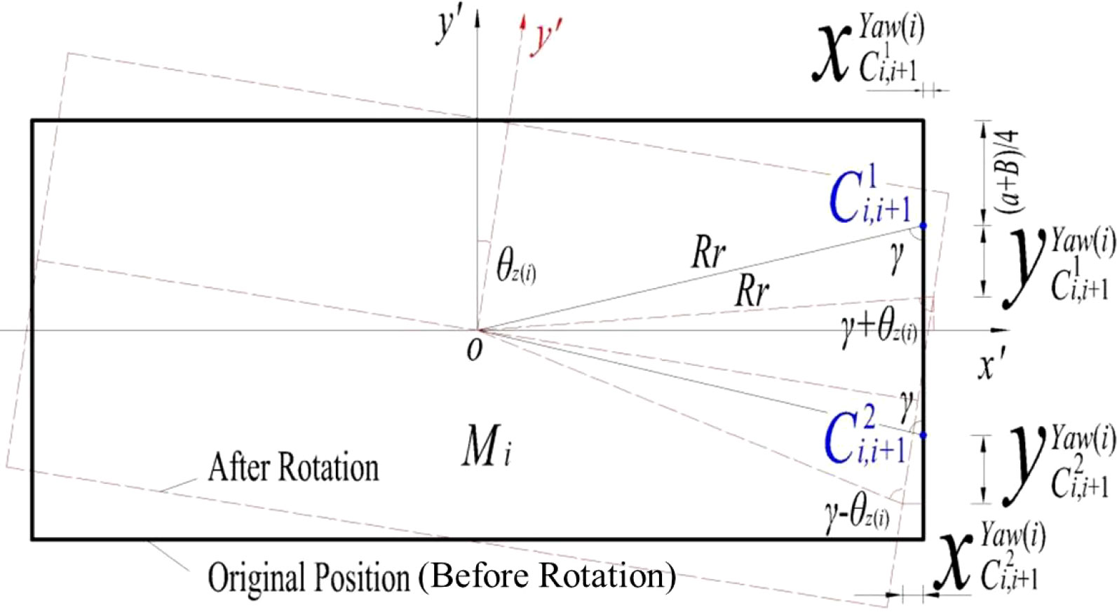
Figure 11 Yaw rotation.

(a) x’ direction:

$\begin{array}{ll}\{\begin{array}{l}\begin{array}{cc}{x}_{C_{i,i+1}^1}^{Yaw(i)}=-Rr[\sin (\gamma +{\theta }_{z(i)})-\sin \gamma ],& x_{C_{i,i+1}^2}^{Yaw(i)}=Rr[\sin \gamma -\sin (\gamma -{\theta }_{z(i)})]\end{array}\\ \begin{array}{cc}\Delta x_{C_{i,i+1}^1}^{Yaw}=-Rr[\sin (\gamma +{\theta }_{z(i+1)})-\sin (\gamma +{\theta }_{z(i)})],& \Delta x_{C_{i,i+1}^2}^{Yaw}=-Rr[\sin (\gamma -{\theta }_{z(i+1)})-\sin (\gamma -{\theta }_{z(i)})]\end{array}\end{array}& (12)\end{array}$

(b) y’ direction:

$\begin{array}{ll}\{\begin{array}{l}\begin{array}{cc}{y}_{C_{i,i+1}^1}^{Yaw(i)}=Rr[\cos \gamma -\cos (\gamma +{\theta }_{z(i)})],& y_{C_{i,i+1}^2}^{Yaw(i)}=Rr[\cos (\gamma -{\theta }_{z(i)})-\cos \gamma ]\end{array}\\ \begin{array}{cc}\Delta y_{C_{i,i+1}^1}^{Yaw}=-Rr[\cos (\gamma +{\theta }_{z(i+1)})-\cos (\gamma +{\theta }_{z(i)})],& \Delta y_{C_{i,i+1}^2}^{Yaw}=Rr[\cos (\gamma -{\theta }_{z(i+1)})-\cos (\gamma -{\theta }_{z(i)})]\end{array}\end{array}& (13)\end{array}$

where $x_{C_{i,i+1}^1}^{Pitch(i)},x_{C_{i,i+1}^1}^{Yaw(i)};y_{C_{i,i+1}^1}^{Roll(i)},y_{C_{i,i+1}^1}^{Yaw(i)};z_{C_{i,i+1}^1}^{Pitch(i)},z_{C_{i,i+1}^1}^{Roll(i)}$ and $x_{C_{i,i+1}^2}^{Pitch(i)},x_{C_{i,i+1}^2}^{Yaw(i)};y_{C_{i,i+1}^2}^{Roll(i)},y_{C_{i,i+1}^2}^{Yaw(i)};z_{C_{i,i+1}^2}^{Pitch(i)},z_{C_{i,i+1}^2}^{Roll(i)}$ are the deformations for $C_{i,i+1}^1$ and $C_{i,i+1}^2$ in the x’, y’, and z’ directions because of the CP-VLFS module’s rotation along the pitch, roll, and yaw, respectively; $\Delta x_{C_{i,i+1}^1}^{Pitch},\Delta x_{C_{i,i+1}^1}^{Yaw};\Delta y_{C_{i,i+1}^1}^{Roll},\Delta y_{C_{i,i+1}^1}^{Yaw};\Delta z_{C_{i,i+1}^1}^{Pitch},\Delta z_{C_{i,i+1}^1}^{Roll}$ and $\Delta x_{C_{i,i+1}^2}^{Pitch},\Delta x_{C_{i,i+1}^2}^{Yaw};\Delta y_{C_{i,i+1}^2}^{Roll},\Delta y_{C_{i,i+1}^2}^{Yaw};\Delta z_{C_{i,i+1}^2}^{Pitch},\Delta z_{C_{i,i+1}^2}^{Roll}$ are the relative deformations for $C_{i,i+1}^1$ and $C_{i,i+1}^2$ ; as well as θ_x(i),θ_y(i),θ_z(i) and θ_x(i+1),θ_y(i+1),θ_z(i+1) are the hydrodynamic response rotational angles of Mi and M_i+1 along the roll, pitch, and yaw.

(3) Total relative deformations of CP-VLFS’s connectors

In summary, the total relative deformations of $C_{i,i+1}^1$ and $C_{i,i+1}^2$ in x’ direction are the sum of the modules’ motion along the surge, pitch, and yaw; those in the y’ direction are the sum of the motion along the sway, roll, and yaw; and those in the z’ direction are the sum of the motion along the heave, roll, and pitch. Therefore, the total relative deformations for connectors in the directions of x’, y’, and z’ are expressed as:

(a) ox’ direction:

$\begin{array}{ll}\{\begin{array}{l}\Delta x_{C_{i,i+1}^1}=\Delta x_{C_{i,i+1}^1}^{Surge}+\Delta x_{C_{i,i+1}^1}^{Pitch}+\Delta x_{C_{i,i+1}^1}^{Yaw}\\ \Delta x_{C_{i,i+1}^2}=\Delta x_{C_{i,i+1}^2}^{Surge}+\Delta x_{C_{i,i+1}^2}^{Pitch}+\Delta x_{C_{i,i+1}^2}^{Yaw}\end{array}& (14)\end{array}$

(b) oy’ direction:

$\begin{array}{ll}\{\begin{array}{l}\Delta y_{C_{i,i+1}^1}=\Delta y_{C_{i,i+1}^1}^{Sway}+\Delta y_{C_{i,i+1}^1}^{Roll}+\Delta y_{C_{i,i+1}^1}^{Yaw}\\ \Delta y_{C_{i,i+1}^2}=\Delta y_{C_{i,i+1}^2}^{Sway}+\Delta y_{C_{i,i+1}^2}^{Roll}+\Delta y_{C_{i,i+1}^2}^{Yaw}\end{array}& (15)\end{array}$

(c) oz’ direction:

$\begin{array}{ll}\{\begin{array}{l}\Delta z_{C_{i,i+1}^1}=\Delta z_{C_{i,i+1}^1}^{Heave}+\Delta z_{C_{i,i+1}^1}^{Roll}+\Delta z_{C_{i,i+1}^1}^{Pitch}\\ \Delta z_{C_{i,i+1}^2}=\Delta z_{C_{i,i+1}^2}^{Heave}+\Delta z_{C_{i,i+1}^2}^{Roll}+\Delta z_{C_{i,i+1}^2}^{Pitch}\end{array}& (16)\end{array}$

where the expressions of the relative deformations for $C_{i,i+1}^1$ and $C_{i,i+1}^2$ in different directions are determined from Eqs. (5) to (13).

2.2.2 Formulas for the constraint loads of connectors

On the basis of Hook’s law, the Eqs. (14)-(16) are inserted into Eq. (1) to confirm the formulas for calculating the constraint loads of $C_{i,i+1}^1$ and $C_{i,i+1}^2$ in the x’, y’, and z’ directions, and the time-varying characteristics for the motion displacements of CP-VLFS modules are considered, as follows:

$\begin{array}{ll}\begin{array}{l}{C}_{i,i+1}^1:\\ \{\begin{array}{l}{F}_{cx}^{C_{i,i+1}^1}(t)=k_{x{C}_{i,i+1}^1}·\Delta x_{C_{i,i+1}^1}(t)=k_{x{C}_{i,i+1}^1}·\{[{\xi }_{x(i+1)}(t)-{\xi }_{x(i)}(t)]-r[\sin (\alpha +{\theta }_{y(i+1)}(t))-\sin (\alpha +{\theta }_{y(i)}(t))]\\ -Rr[\sin (\gamma +{\theta }_{z(i+1)}(t))-\sin (\gamma +{\theta }_{z(i)}(t))]\}\\ F_{cy}^{C_{i,i+1}^1}(t)=k_{y{C}_{i,i+1}^1}·\Delta y_{C_{i,i+1}^1}(t)=k_{y{C}_{i,i+1}^1}·\{[{\xi }_{y(i+1)}(t)-{\xi }_{y(i)}(t)]-R[\sin (\beta +{\theta }_{x(i+1)}(t))-\sin (\beta +{\theta }_{x(i)}(t))]\\ -Rr[\cos (\gamma +{\theta }_{z(i+1)})-\cos (\gamma +{\theta }_{z(i)})]\}\\ F_{cz}^{C_{i,i+1}^1}(t)=k_{z{C}_{i,i+1}^1}·\Delta z_{C_{i,i+1}^1}(t)=k_{z{C}_{i,i+1}^1}·\{[{\xi }_{z(i+1)}(t)-{\xi }_{z(i)}(t)]-R[\cos (\beta +{\theta }_{x(i+1)}(t))-\cos (\beta +{\theta }_{x(i)}(t))]\\ -r[\cos (\alpha +{\theta }_{y(i+1)}(t))-\cos (\alpha +{\theta }_{y(i)}(t))]\}\end{array}\end{array}& (17)\end{array}$

$\begin{array}{ll}\begin{array}{l}{C}_{i,i+1}^2:\\ \{\begin{array}{l}{F}_{cx}^{C_{i,i+1}^2}(t)=k_{x{C}_{i,i+1}^2}·\Delta x_{C_{i,i+1}^2}(t)=k_{x{C}_{i,i+1}^2}·\{[{\xi }_{x(i+1)}(t)-{\xi }_{x(i)}(t)]-r[\sin (\alpha +{\theta }_{y(i+1)}(t))-\sin (\alpha +{\theta }_{y(i)}(t))]\\ -Rr[\sin (\gamma -{\theta }_{z(i+1)}(t))-\sin (\gamma -{\theta }_{z(i)}(t))]\}\\ F_{cy}^{C_{i,i+1}^2}(t)=k_{y{C}_{i,i+1}^2}·\Delta y_{C_{i,i+1}^2}(t)=k_{y{C}_{i,i+1}^2}·\{[{\xi }_{y(i+1)}(t)-{\xi }_{y(i)}(t)]+R[\sin (\beta -{\theta }_{x(i+1)}(t))-\sin (\beta -{\theta }_{x(i)}(t))]\\ +Rr[\cos (\gamma -{\theta }_{z(i+1)}(t))-\cos (\gamma -{\theta }_{z(i)}(t))]\}\\ F_{cz}^{C_{i,i+1}^2}(t)=k_{z{C}_{i,i+1}^2}·\Delta z_{C_{i,i+1}^2}(t)=k_{z{C}_{i,i+1}^2}·\{[{\xi }_{z(i+1)}(t)-{\xi }_{z(i)}(t)]-R[\cos (\beta -{\theta }_{x(i+1)}(t))-\cos (\beta -{\theta }_{x(i)}(t))]\\ -r[\cos (\alpha +{\theta }_{y(i+1)}(t))-\cos (\alpha +{\theta }_{y(i)}(t))]\}\end{array}\end{array}& (18)\end{array}$

where $\begin{array}{ccc}{k}_{x{C}_{i,i+1}^1},& k_{y{C}_{i,i+1}^1},& k_{z{C}_{i,i+1}^1}\end{array}$ and $\begin{array}{ccc}{k}_{x{C}_{i,i+1}^2},& k_{y{C}_{i,i+1}^2},& k_{z{C}_{i,i+1}^2}\end{array}$ are the stiffnesses of $C_{i,i+1}^1$ and $C_{i,i+1}^2$ in the x’, y’, and z’ directions. In Eqs. (17) and (18), the unknowns are only the hydrodynamic response displacements for M_i and M_i+1 in the six motion directions ξ_x(i+1)(t), ξ_y(i+1)(t), ξ_z(i+1)(t), θ_x(i+1)(t), θ_y(i+1)(t), θ_z(i+1)(t), ξ_x(i)(t), ξ_y(i)(t), ξ_z(i)(t), θ_x(i)(t), θ_y(i)(t), θ_z(i)(t). These values all vary with time and can thus be solved by the equations in Eq. (4), along with Eqs. (17) and (18), to evaluate the constraint loads of $C_{i,i+1}^1$ and $C_{i,i+1}^2$.

2.2.3 Constraint load matrix of CP-VLFS’s connectors

Expressions of the hydrodynamic coefficient matrix, RIW excitation force matrix, as well as constraint load matrix of CP-VLFS’s connectors in the six DOF directions within Eq. (4) should be derived to solve and obtain the hydrodynamic response results for CP-VLFS modules. Eqs. (17) and (18) denote the formulas for the total constraint loads of $C_{i,i+1}^1$ and $C_{i,i+1}^2$ in directions of x’, y’, and z’ are different from the expressions for the connectors’ constraint loads in the six DOF directions. According to Sections 2.2.1 and 2.2.2, the expressions for the constraint load matrix and its corresponding elements within Eq. (4) are as follows:

$\begin{array}{ll}\{F_{ci}(t)\}={[\begin{array}{cccccc}{F}_{ci(j=2)}^{Surge}(t)& F_{ci(j=2)}^{Sway}(t)& F_{ci(j=2)}^{Heave}(t)& F_{ci(j=2)}^{Roll}(t)& F_{ci(j=2)}^{Pitch}(t)& F_{ci(j=2)}^{Yaw}(t)\end{array}]}^{\text{T}}& (19)\end{array}$

$\begin{array}{ll}\{\begin{array}{l}{F}_{ci(j=2)}^{Surge}(t)=k_{x{C}_{i,i+1}^1}·\Delta x_{C_{i,i+1}^1}^{Surge}+k_{x{C}_{i,i+1}^2}·\Delta x_{C_{i,i+1}^2}^{Surge}=(k_{x{C}_{i,i+1}^1}+k_{x{C}_{i,i+1}^2})·[{\xi }_{x(i+1)}(t)-{\xi }_{x(i)}(t)]\\ F_{ci(j=2)}^{Sway}(t)=k_{y{C}_{i,i+1}^1}·\Delta y_{C_{i,i+1}^1}^{Sway}+k_{y{C}_{i,i+1}^2}·\Delta y_{C_{i,i+1}^2}^{Sway}=(k_{y{C}_{i,i+1}^1}+k_{y{C}_{i,i+1}^2})·[{\xi }_{y(i+1)}(t)-{\xi }_{y(i)}(t)]\\ F_{ci(j=2)}^{Heave}(t)=k_{z{C}_{i,i+1}^1}·\Delta z_{C_{i,i+1}^1}^{Heave}+k_{z{C}_{i,i+1}^2}·\Delta z_{C_{i,i+1}^2}^{Heave}=(k_{z{C}_{i,i+1}^1}+k_{z{C}_{i,i+1}^2})·[{\xi }_{z(i+1)}(t)-{\xi }_{z(i)}(t)]\\ F_{ci(j=2)}^{Roll}(t)=k_{y{C}_{i,i+1}^1}·\Delta y_{C_{i,i+1}^1}^{Roll}+k_{y{C}_{i,i+1}^2}·\Delta y_{C_{i,i+1}^2}^{Roll}+k_{z{C}_{i,i+1}^2}·\Delta z_{C_{i,i+1}^1}^{Roll}+k_{z{C}_{i,i+1}^1}·\Delta z_{C_{i,i+1}^2}^{Roll}\\ =-k_{y{C}_{i,i+1}^1}·R[\sin (\beta +{\theta }_{x(i+1)}(t))-\sin (\beta +{\theta }_{x(i)}(t))]\\ +k_{y{C}_{i,i+1}^2}·R[\sin (\beta -{\theta }_{x(i+1)}(t))-\sin (\beta -{\theta }_{x(i)}(t))]\\ -k_{z{C}_{i,i+1}^2}·R[\cos (\beta +{\theta }_{x(i+1)}(t))-\cos (\beta +{\theta }_{x(i)}(t))]\\ -k_{z{C}_{i,i+1}^1}·R[\cos (\beta -{\theta }_{x(i+1)}(t))-\cos (\beta -{\theta }_{x(i)}(t))]\\ F_{ci(j=2)}^{Pitch}(t)=k_{x{C}_{i,i+1}^1}·\Delta x_{C_{i,i+1}^1}^{Pitch}+k_{x{C}_{i,i+1}^2}·\Delta x_{C_{i,i+1}^2}^{Pitch}+k_{z{C}_{i,i+1}^1}·\Delta z_{C_{i,i+1}^1}^{Pitch}+k_{z{C}_{i,i+1}^2}·\Delta z_{C_{i,i+1}^2}^{Pitch}\\ =-(k_{x{C}_{i,i+1}^1}+k_{x{C}_{i,i+1}^2})·r[\sin (\alpha +{\theta }_{y(i+1)}(t))-\sin (\alpha +{\theta }_{y(i)}(t))]\\ -(k_{z{C}_{i,i+1}^1}+k_{z{C}_{i,i+1}^2})·r[\cos (\alpha +{\theta }_{y(i+1)}(t))-\cos (\alpha +{\theta }_{y(i)}(t))]\\ F_{ci(j=2)}^{Yaw}(t)=k_{x{C}_{i,i+1}^1}·\Delta x_{C_{i,i+1}^1}^{Yaw}+k_{x{C}_{i,i+1}^2}·\Delta x_{C_{i,i+1}^2}^{Yaw}+k_{y{C}_{i,i+1}^1}·\Delta y_{C_{i,i+1}^1}^{Yaw}+k_{y{C}_{i,i+1}^2}·\Delta y_{C_{i,i+1}^2}^{Yaw}\\ =-k_{x{C}_{i,i+1}^1}·Rr[\sin (\gamma +{\theta }_{z(i+1)}(t))-\sin (\gamma +{\theta }_{z(i)}(t))]\\ -k_{x{C}_{i,i+1}^2}·Rr[\sin (\gamma -{\theta }_{z(i+1)}(t))-\sin (\gamma -{\theta }_{z(i)}(t))]\\ -k_{y{C}_{i,i+1}^1}·Rr[\cos (\gamma +{\theta }_{z(i+1)}(t))-\cos (\gamma +{\theta }_{z(i)}(t))]\\ +k_{y{C}_{i,i+1}^2}·Rr[\cos (\gamma -{\theta }_{z(i+1)}(t))-\cos (\gamma -{\theta }_{z(i)}(t))]\end{array}& (20)\end{array}$

where the symbols are the same as above.

2.3 Hydrodynamic coefficients, RIW excitation force, and hydrodynamic equation solution

2.3.1 Hydrodynamic coefficient matrix

The expressions for the hydrodynamic coefficient matrix and the elements of a single CP-VLFS module within Eq. (4) are given directly, and the derivation of each expression is provided in literatures (Li et al., 2017; Wu et al., 2017).

(1) Mass matrix

The expression of the mass matrix for CP-VLFS module is as follows:

$\begin{array}{ll}[M_s]=diag[\begin{array}{cccccc}{m}_s& m_s& m_s& I_{xx}& I_{yy}& I_{zz}\end{array}]& (21)\end{array}$

where diag[·] denotes the diagonal matrix; m_s denotes the mass of CP-VLFS module; and I_xx, I_yy, and I_zz are the rotational inertias along the directions of roll, pitch and yaw, respectively.

(2) Added mass matrix

The added mass matrix of CP-VLFS module can be quantized as follows according to the strip theory of ship mechanics (Zhao et al., 2014a):

$\begin{array}{ll}[M_f(t)]=diag[\begin{array}{cccccc}{m}_{fx}^{Surge}(t)& m_{fy}^{Sway}(t)& m_{fz}^{Heave}& m_{f\theta x}^{Roll}(t)& m_{f\theta y}^{Ptich}(t)& m_{f\theta z}^{Yaw}\end{array}]& (22)\end{array}$

where $m_{fx}^{Surge}(t)$, $m_{fy}^{Sway}(t)$, $m_{fz}^{Heave}$, $m_{f\theta x}^{Roll}(t)$, $m_{f\theta y}^{Pitch}(t)$, and $m_{f\theta z}^{Yaw}$ denote the structural added mass of CP-VLFS module in six DOF directions, whose expressions are shown in literatures (Li et al., 2017), as expressed:

$\begin{array}{ll}\begin{array}{cc}{m}_{fx}^{Surge}(t)=(\frac{\rho \pi D^2}{4})·{\displaystyle \sum _{i=1}^k{z}_{s(i)}(t)}+k^{\text{'}}·C_m^{*}·\rho ·l·a·b,& C_m^{*}=C_m^{*}(\frac{l}{a})\end{array}& (23)\end{array}$

$\begin{array}{ll}\begin{array}{cc}{m}_{fy}^{Sway}(t)=(\frac{\rho \pi D^2}{4})·{\displaystyle \sum _{i=1}^k{z}_{s(i)}(t)}+k^{\text{'}}·C_m^{*}·\rho ·l·a·b,& C_m^{*}=C_m^{*}(\frac{a}{b})\end{array}& (24)\end{array}$

$\begin{array}{ll}\begin{array}{cc}{m}_{fz}^{Heave}=k^{\text{'}}·C_m^{*}·\rho ·l·a·b,& C_m^{*}=C_m^{*}(\frac{b}{a})\end{array}& (25)\end{array}$

$\begin{array}{ll}\begin{array}{cc}{m}_{f\theta x}^{Roll}(t)=(\frac{\rho \pi D^2}{12})·{\displaystyle \sum _{i=1}^k{z}_{s(i)}^3(t)}+\frac{k^{\text{'}}}{12}·C_m^{*}·\rho ·b·l·a^3,& C_m^{*}=C_m^{*}(\frac{b}{l})\end{array}& (26)\end{array}$

$\begin{array}{ll}\begin{array}{cc}{m}_{f\theta y}^{Pitch}(t)=(\frac{\rho \pi D^2}{12})·{\displaystyle \sum _{i=1}^k{z}_{s(i)}^3(t)}+\frac{k^{\text{'}}}{12}·C_m^{*}·\rho ·a·b·l^3,& C_m^{*}=C_m^{*}(\frac{b}{a})\end{array}& (27)\end{array}$

$\begin{array}{ll}\begin{array}{cc}{m}_{f\theta z}^{Yaw}=\frac{k^{\text{'}}}{12}·C_m^{*}·\rho ·a·b·l^3,& C_m^{*}=C_m^{*}(\frac{a}{b})\end{array}& (28)\end{array}$

where ρ is the density of sea water; the symbols of z_s, a, b, l, D are the geometric parameters for the CP-VLFS module, which can be seen in Figures 6 and 7; i means an arbitrary column; $C_m^{*}$ is an impact coefficient, and $C_m^{*}=[0.8862+0.1938·(s_1/s_2)]/(s_1/s_2)$, as elaborated in Figure A.3 of Wu et al., 2017. k and k’ are the number of columns and pontoons for a single CP-VLFS module, respectively.

(3) Damping coefficient matrix

The damping coefficients of CP-VLFS module are expressed as follows:

$\begin{array}{ll}[C_f]=diag[\begin{array}{cccccc}{c}_f^{Surge}& c_f^{Sway}& c_f^{Heave}& c_f^{Roll}& c_f^{Pitch}& c_f^{Yaw}\end{array}]& (29)\end{array}$

where $c_f^{Surge}$, $c_f^{Sway}$, $c_f^{Heave}$, $c_f^{Roll}$, $c_f^{Pitch}$, and $c_f^{Yaw}$denote the damping coefficients for CP-VLFS module in six directions, as elaborated in literature (Wu et al., 2017), i.e., c_f>^Surge= 1.14×10⁷, c_f>^Sway= 3.30×10⁷, c_f>^Heave= 2.52×10⁷, c_f>^Roll= 8.80×10⁷, c_f>^Pitch= 6.35×10⁷, c_f>^Yaw= 1.07×10⁷.

(4) Static resilience coefficient matrix

The resilience of floating body structure happens in the directions of heave, roll and pitch (Zhao et al., 2014b), and the static resilience coefficient matrix of CP-VLFS module is as follows:

$\begin{array}{ll}[K_f(t)]=diag[\begin{array}{cccccc}0& 0& k_f^{Heave}& k_f^{Roll}(t)& k_f^{Pitch}(t)& 0\end{array}]& (30)\end{array}$

where $k_f^{Heave}$, $k_f^{Roll}(t)$, and $k_f^{Pitch}(t)$ are the static resilience coefficients for CP-VLFS module in the directions of heave, roll and pitch, whose expressions were acquired in literatures (Li et al., 2017), as expressed:

$\begin{array}{ll}{k}_f^{Heave}=2·\rho ·g·\pi ·D^2& (31)\end{array}$

$\begin{array}{ll}\begin{array}{l}{k}_f^{Roll}(t)=\rho ·g·\left\{{\displaystyle \sum _{i=1}^{k\text{'}}[\frac{\pi D^2}{4}·z_{s(i)}(t)]}+2·a·b·l\right\}·\left\{\frac{{\displaystyle \sum _{i=1}^{k\text{'}}[\frac{\pi D^2}{8}·z_{s(i)}^2(t)]}+2·a·b·l·z_m}{{\displaystyle \sum _{i=1}^{k\text{'}}[\frac{\pi D^2}{4}·z_{s(i)}(t)]}+2·a·b·l}-z_G\right\}\\ +\rho ·g·\left\{2·\pi ·D^2·[{(\frac{B}{2})}^2+{(\frac{D}{4})}^2]\right\}\end{array}& (32)\end{array}$

$\begin{array}{ll}\begin{array}{l}{k}_f^{Pitch}(t)=\rho ·g·\left\{{\displaystyle \sum _{i=1}^{k\text{'}}[\frac{\pi D^2}{4}{z}_{s(i)}(t)]}+2·a·b·l\right\}·\left\{\frac{{\displaystyle \sum _{i=1}^{k\text{'}}[\frac{\pi D^2}{8}·z_{s(i)}^2(t)]}+2·a·b·l·z_m}{{\displaystyle \sum _{i=1}^{k\text{'}}[\frac{\pi D^2}{4}·z_{s(i)}(t)]}+2·a·b·l}-z_G\right\}\\ +\rho ·g·[\pi ·D^2·(l_1^2+l_2^2+\frac{D^2}{8})]\end{array}& (33)\end{array}$

where ρ is the density of sea water; g means the gravitational acceleration; the symbols of z_s, a, b, l, D, z_m, z_G, B, l₁, l₂ are all the geometric parameters of CP-VLFS module, as seen in Figures 6 and 7.

2.3.2 Excitation force of RIW

This paper focuses on the development of a rapid and high-efficiency method to obtain the hydrodynamic constraint loads of CP-VLFS’s connectors at HSSs The significant components for CP-VLFS module, including the columns and the pontoons, are both treated as small-scale ones via comparing them with very large wavelengths at HSSs. By means of the aforementioned considerations, the Morison theory can be used to quantify the forces of RIW on CP-VLFSs at the stage of preliminary design. For this paper’s studies, the Morison equation of floating body is utilized to quantify the excitation forces of RIW at HSSs (Nie and Liu, 2002), which can extremely improve the efficiency of solving while ensuring sufficiently precise results.

The derivation process of floating body Morison theory and the excitation force of RIW on CP-VLFS module are elaborated in detail in literatures of Wu et al. 2016b. Summarily, the RIW excitation force matrix for CP-VLFS module is written as follows:

$\begin{array}{ll}\{F_w(t)\}={[\begin{array}{cccccc}{F}_w^{Surge}(t)& F_w^{Sway}(t)& F_w^{Heave}(t)& M_w^{Roll}(t)& M_w^{Pitch}(t)& M_w^{Yaw}(t)\end{array}]}^{\text{T}}& (34)\end{array}$

where $F_w^{Surge}(t)$, $F_w^{Sway}(t)$, $F_w^{Heave}(t)$, $M_w^{Roll}(t)$, $M_w^{Pitch}(t)$, and $M_w^{Yaw}(t)$ denote the RIW excitation force of CP-VLFS module in the motion directions of six DOFs, i.e., surge, sway, heave, roll, pitch, and yaw. Due to the complex derivation process of wave forces on CP-VLFS module, the tedious expressions of RIW forces in six DOF directions were elaborated in details via Wu et al. 2016b and Wu et al. 2017.

Every single CP-VLFS module connects with each other depending on the specially designed flexible connectors installed on the top platform of CP-VLFS, but the components of columns and pontoons under the water are disconnected with others. When the waves propagate along a certain direction, the fluid field around the floating structure changes because of the shadowing effect among adjacent modules (Yao and Shi, 2022). The excitation forces of RIW acting on multi-columns show differences from the single one due to the shadowing effects when the RIWs propagated from the front to the back (Zhang et al., 2013), and the shadowing phenomenon among different CP-VLFS modules’ columns is certainly considered by this paper. The approach is similar to the method for evaluating the wave forces acting on the pile group effects. Firstly, the excitation forces of RIW acting on a single column are assessed via using the Morison theory for floating body; and then, the RIW forces acting on groups of CP-VLFS modules’ columns are equal to the estimation results of single one multiplied via the coefficients of shadowing effect K_w, which the empirical function for the K_w(L/D)=0.7167·exp[0.0813·(L/D)] on the basis of Bonakdar and Oumeraci, 2015. It is worth noting that the shadowing effects of groups of columns can be ignored when L/D>4, where L is the separation distance of two adjacent columns and D is the diameter of the column.

2.3.3 Hydrodynamic equation solution

According to Eqs. (17) and (18), the hydrodynamic constraint loads of connectors have something to do with the two adjacent CP-VLFS modules of M_i and M_i+1. Twelve hydrodynamic equations of M_i and M_i+1 are united to solve the time-domain hydrodynamic responses of M_i and M_i+1. The general hydrodynamic equations for M_i and M_i+1 are expressed as follows:

$\begin{array}{ll}\begin{array}{cc}{M}_i:& ([M_s]+[M_f^i(t)])\left\{{\ddot{X}}_i(t)\right\}+[C_f^i(t)]\left\{{\dot{X}}_i(t)\right\}+[K_f^i(t)]\left\{X_i(t)\right\}=\left\{F_w^i(t)\right\}+\left\{F_c^i(t)\right\}\end{array}& (35)\end{array}$

$\begin{array}{ll}\begin{array}{cc}{M}_{i+1}:& ([M_s]+[M_f^{i+1}(t)])\left\{{\ddot{X}}_{i+1}(t)\right\}+[C_f^{i+1}(t)]\left\{{\dot{X}}_{i+1}(t)\right\}+[K_f^{i+1}(t)]\left\{X_{i+1}(t)\right\}=\left\{F_w^{i+1}(t)\right\}+\left\{F_c^{i+1}(t)\right\}\end{array}& (36)\end{array}$

where Eqs. (35) and (36) respectively include six independent equations for M_i and M_i+1. {X_i(t)} and {X_i+1(t)} denote the column vectors of the hydrodynamic response results for M_i and M_i+1, which are expressed as follows:

$\begin{array}{ll}\left\{X_i(t)\right\}={\left\{\begin{array}{cccccc}{\xi }_{x(i)}(t)& {\xi }_{y(i)}(t)& {\xi }_{z(i)}(t)& {\theta }_{x(i)}(t)& {\theta }_{y(i)}(t)& {\theta }_{z(i)}(t)\end{array}\right\}}^{\text{T}}& (37)\end{array}$

$\begin{array}{ll}\left\{X_i{+}_1(t)\right\}={\left\{\begin{array}{cccccc}{\xi }_{x(i+1)}(t)& {\xi }_{y(i+1)}(t)& {\xi }_{z(i+1)}(t)& {\theta }_{x(i+1)}(t)& {\theta }_{y(i+1)}(t)& {\theta }_{z(i+1)}(t)\end{array}\right\}}^{\text{T}}& (38)\end{array}$

where these elements within the column vectors of Eqs. (37) and (38) denote the hydrodynamic response displacements ξ and rotational angles θ for M_i and M_i+1 in the directions of the six DOFs. Because these derived matrices include the constraint loads matrix (Eqs. (19)-(20)), hydrodynamic coefficients matrix (Eqs. (21)-(33)), and wave excitation force matrix (Eq. (34)), we can insert their elements into Eqs. (35) and (36) to solve these 12 equations and obtain hydrodynamic response results based on the method of Runge-Kutta in four-orders (Zhao et al., 2014a). Ultimately, the results of hydrodynamic response within Eqs. (37) and (38) are inserted into Eqs. (17) and (18), respectively, to evaluate the hydrodynamic constraint loads of $C_{i,i+1}^1$ and $C_{i,i+1}^2$ in the directions of x’, y’, and z’.

This paper’s estimation method is suitable for the hydrodynamic constraint loads of CP-VLFS’s connectors. Because the mooring and anchoring facilities for CP-VLFSs are unconsidered stated in Section 2.1, hence, the restraining boundary conditions for the CP-VLFS model are restricted via using the initial motion displacements of CP-VLFS, which can be defined the structural motion positions as 0 at the beginning of each calculated time step t_step during the equations solving. The aforementioned approach is reasonably utilized to simulate the functions of dynamic positioning systems (DPSs) for CP-VLFS that are elaborated in Wu et al. 2017. Finally, the numerical results correspond well with the method of PFT and the experimental measurements in following Sections.

3 Case study

3.1 Modules and connectors of CP-VLFS

According to the prototype of CP-VLFS reported by Ding et al. (2005), there are two connectors installing on the top platform of two adjacent CP-VLFS’s modules. The stiffnesses for CP-VLFS’s connectors in the directions of x, y, and z were kept constant, with values of k_x=1.00×10⁹ N/m, k_y=1.00×10¹² N/m, and k_z=1.00×10¹² N/m, respectively.

Figure 12 shows the geometric scales of CP-VLFS module and the connectors’ installation positions. A numerical model of CP-VLFS with three-modules and four-connectors in this paper at sea state six (SS6) is regarded as a case to explore the accuracy of this paper’s proposed high-efficiency estimation method for the hydrodynamic constraint loads of connectors. Figure 13 shows the conceptual design of three-module-connector model, and M₁, M₂, and M₃ denote each single module; C₁, C₂, C₃, and C₄ denote each connector between two adjacent modules.

FIGURE 12

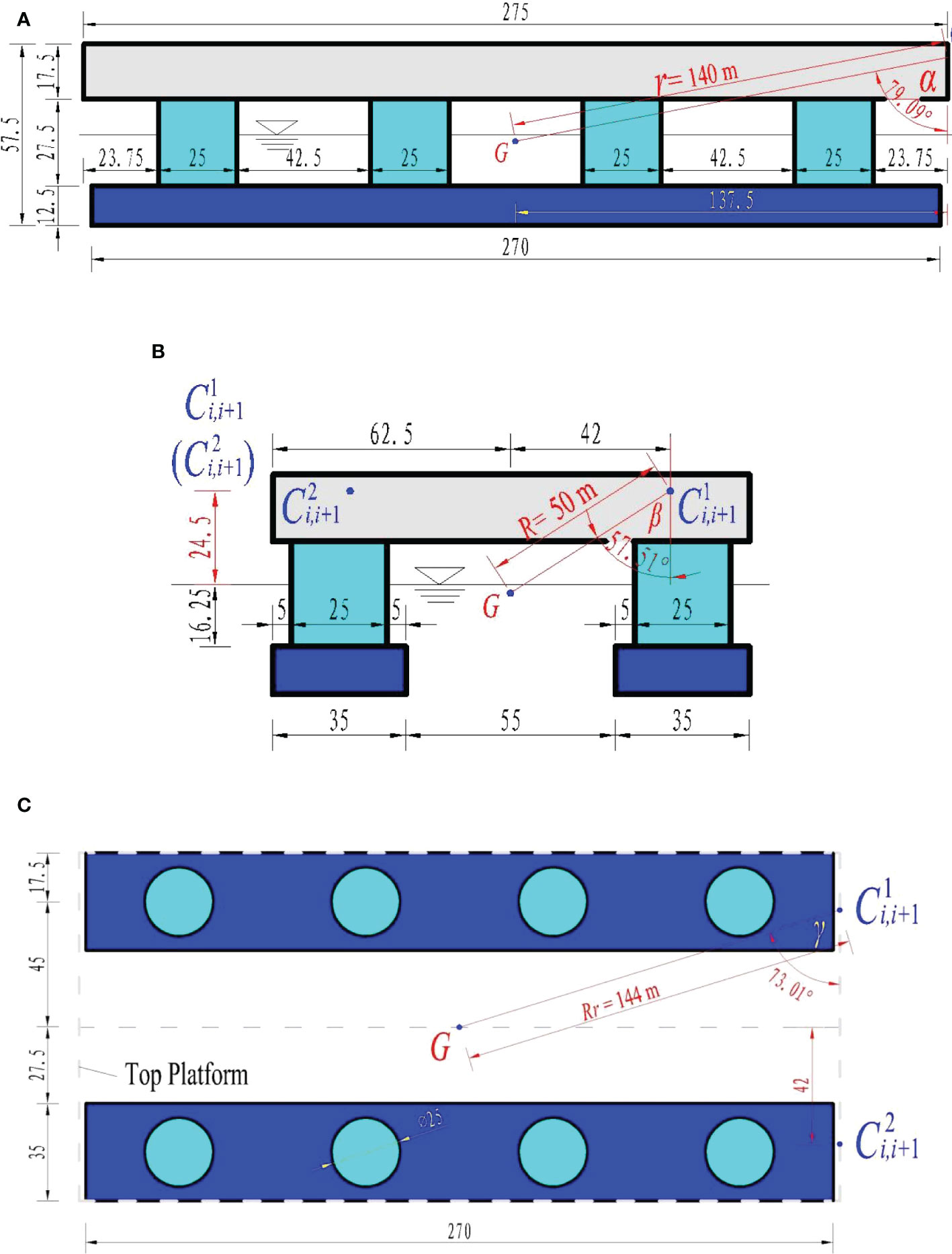
Figure 12 Conceptual design of CP-VLFS module and the connectors’ installation sites (units: m): (A) ox’z’ plane; (B) oy’z’ plane; (C) ox’y’ plane.

FIGURE 13

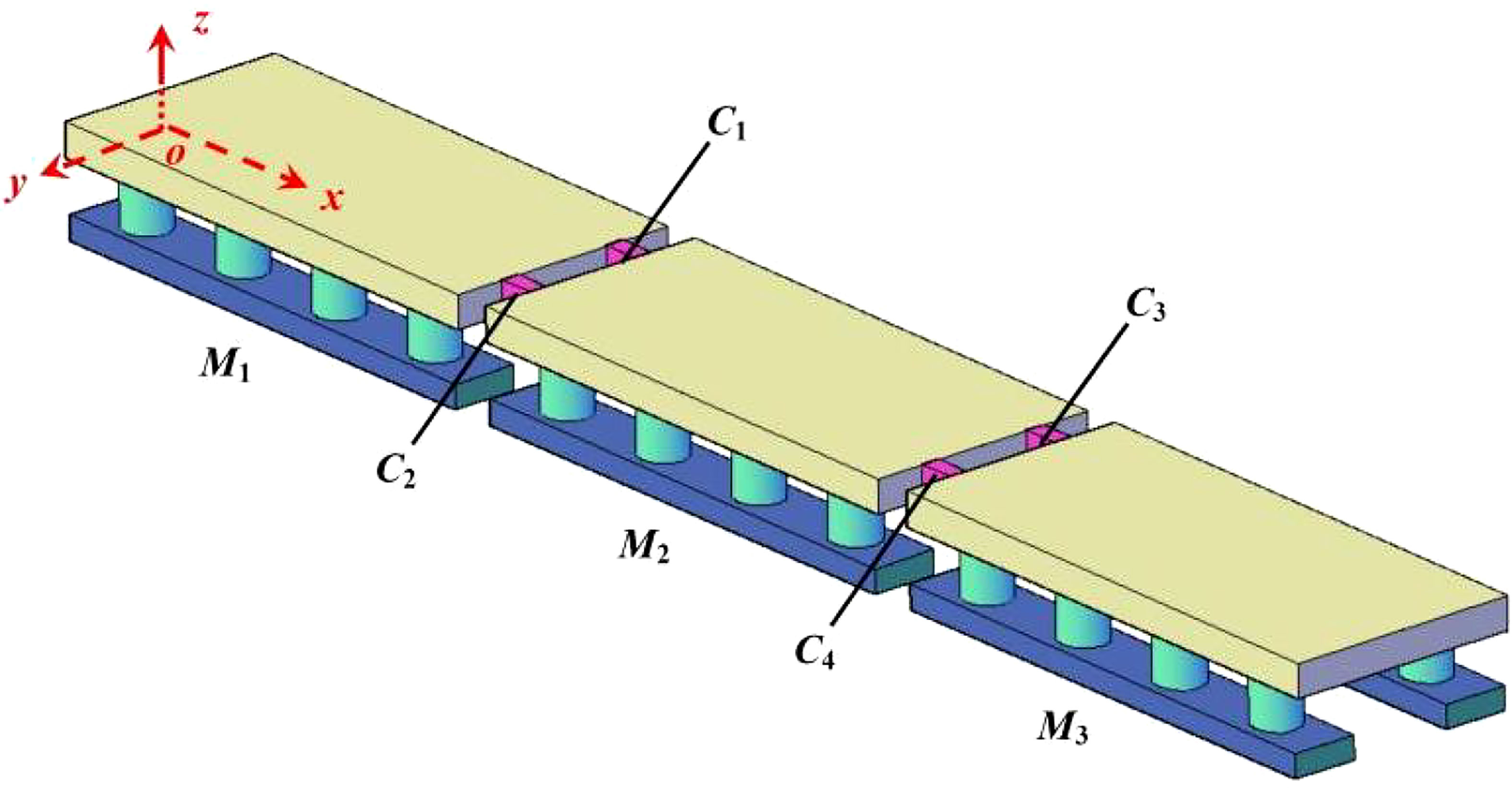
Figure 13 Numerical model of CP-VLFS with three-modules and four-connectors.

3.2 Random irregular wave field

The wave spectral density function S(ω) and the statistical parameters of wave at HSSs are vital when simulating random and irregular wave fields. To validate this paper’s high-efficiency method, the wave spectrum of Bretschneider is utilized to simulate the RIW field at SS6 on the surface of the North Pacific Ocean. The spectral density function is as follows:

$\begin{array}{ll}S(\omega )=\frac{1.25}{4}·{\left(\frac{2\pi }{T_p}\right)}^4·{\omega }^{-5}·H_s^2·\exp \left[-1.25·{\left(\frac{2\pi }{T_p\omega }\right)}^4\right]& (39)\end{array}$

where H_s is the significant wave height; T_p is the spectral peak period; ω is the circular frequency. H_s(SS6)=5 m, T_p(SS6)=12.4 s, and ω(SS6)=0.364-1.307 rad/s. The surface of RIW at SS6 in arbitrary time can be simulated in OXYZ on the basis of aforementioned statistical parameters.

3.3 Results analysis and discussion

According to the aforementioned computational conditions and this paper’s high-efficiency method, the hydrodynamic constraint loads of CP-VLFS’s connectors in time-domain are determined under various wave angles, RIW excitation forces at SS6. The duration for an entirely stable sea state is maintained for nearly 1-2 h (Qiao et al., 2021), hence, this paper defines t=2 h as the computation time.

(1) Time-domain hydrodynamic constraint loads of CP-VLFS’s connectors

The time-domain hydrodynamic constraint loads of C₁ and C₃ in the directions of x, y, and z are plotted in Figures 14 and 15. The results of C₂ and C₄ are similar to those of C₁ and C₃ due to the bisymmetry of CP-VLFS’s module. Therefore, the C₁ and C₃ are treated as the representatives to exploring the variation trend of time-domain hydrodynamic constraint loads on connectors of CP-VLFS. Figures 14 and 15 shows the calculated results as the time variations from t=0 s to 200 s. Meanwhile, the wave angles are set to δ=0°, 15°, 30°, 45°, 60°, 75°, 85°, and 90° to facilitate the following verification of the hydrodynamic results in this paper.

FIGURE 14

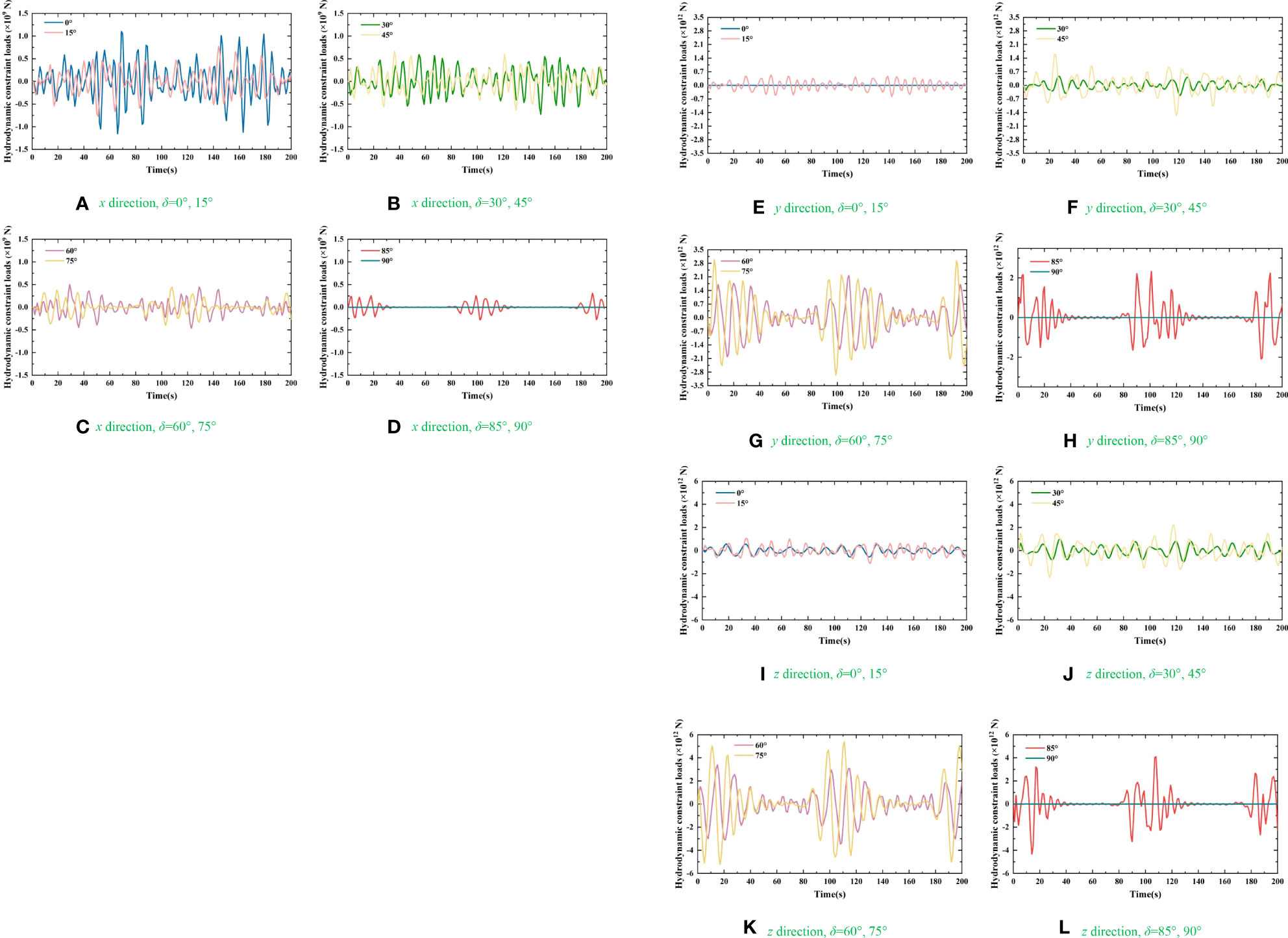
Figure 14 Time-domain hydrodynamic constraint loads of C₁: (A) x direction, δ=0°, 15°; (B) x direction, δ=30°, 45°; (C) x direction, δ=60°, 75°; (D) x direction, δ=85°, 90°; (E) y direction, δ=0°, 15°; (F) y direction, δ=30°, 45°; (G) y direction, δ=60°, 75°; (H) y direction, δ=85°, 90°; (I) z direction, δ=0°, 15°; (J) z direction, δ=30°, 45°; (K) z direction, δ=60°, 75°; (L) z direction, δ=85°, 90°.

FIGURE 15

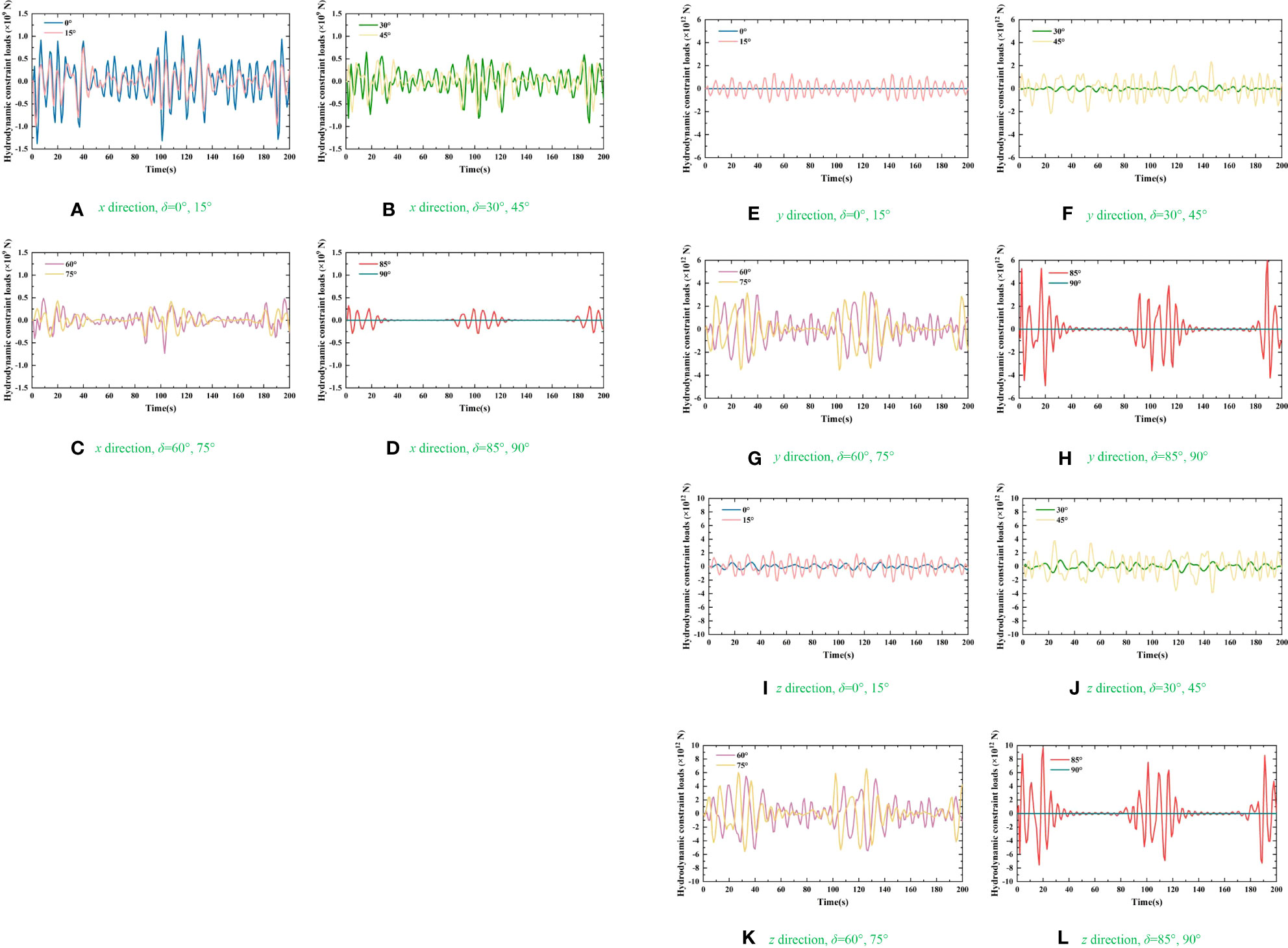
Figure 15 Time-domain hydrodynamic constraint loads of C₃: (A) x direction, δ=0°, 15°; (B) x direction, δ=30°, 45°; (C) x direction, δ=60°, 75°; (D) x direction, δ=85°, 90°; (E) y direction, δ=0°, 15°; (F) y direction, δ=30°, 45°; (G) y direction, δ=60°, 75°; (H) y direction, δ=85°, 90°; (I) z direction, δ=0°, 15°; (J) z direction, δ=30°, 45°; (K) z direction, δ=60°, 75°; (L) z direction, δ=85°, 90°.

Figures 14 and 15 shows random fluctuations in the connectors’ hydrodynamic constraint loads as time elapses. The fluctuation laws between the hydrodynamic results and time for C₁ and C₃ are consistent with each other in directions of x, y, and z, respectively. The fluctuation amplitudes of the constraint loads of C₁ and C₃ in directions of y and z are relatively larger when the t=1-40 s, t=90-150 s, and t=180-200 s. Moreover, the connectors’ estimation results in directions of x, y, and z are the smallest when the wave angle was 90°.

(2) Verification of the results

The statistical values of connectors’ computational hydrodynamic constraint loads by this paper’s rapid and high-efficiency method, including the maximums (Sim-Max), the means (Sim-Mean), the significant values (Sim-SV), as well as the standard deviations (Sim-SD), are compared to the PFT results (PFT-Max, PFT-Mean, PFT-SV, PFT-SD) and those from the physical model experiment (Exp-Max, Exp-Mean, Exp-SV, Exp-SD) under the same preconditions (geometric dimensions of CP-VLFS modules, connectors’ stiffnesses, wave spectrums and angles, sea states, and shadowing effects of CP-VLFS’s components, etc.) to validate the accuracy and credibility of this paper’s proposed method.

The measured results of constraint loads on C₁ and C₃ via using the model experiment were acquired based on the Ding, 2004 and Yu, 2004. During the physical model experiment, the model scale was set as 1:100 according to the Froude’s law of similarity. The experimental physical model of CP-VLFS was included three modules and four connectors, and the geometric dimensions of the CP-VLFS modules and the connectors’ installing position for the experiment are identical to that elaborated in Figures 12 and 13. The experimental photos for physical model of CP-VLFS were shown in Figure 16. During the model experiment, the Bretschneider spectrum was used to simulate the random and irregular wave acting on CP-VLFS model, and the wave angles were considered as δ = 0°, 45°, 75°, 85°, and 90°, as shown in Figure 17.

FIGURE 16

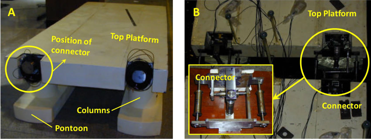
Figure 16 The physical model of CP-VLFS (Ding, 2004 and Yu, 2004): (A) module; (B) connector.

FIGURE 17

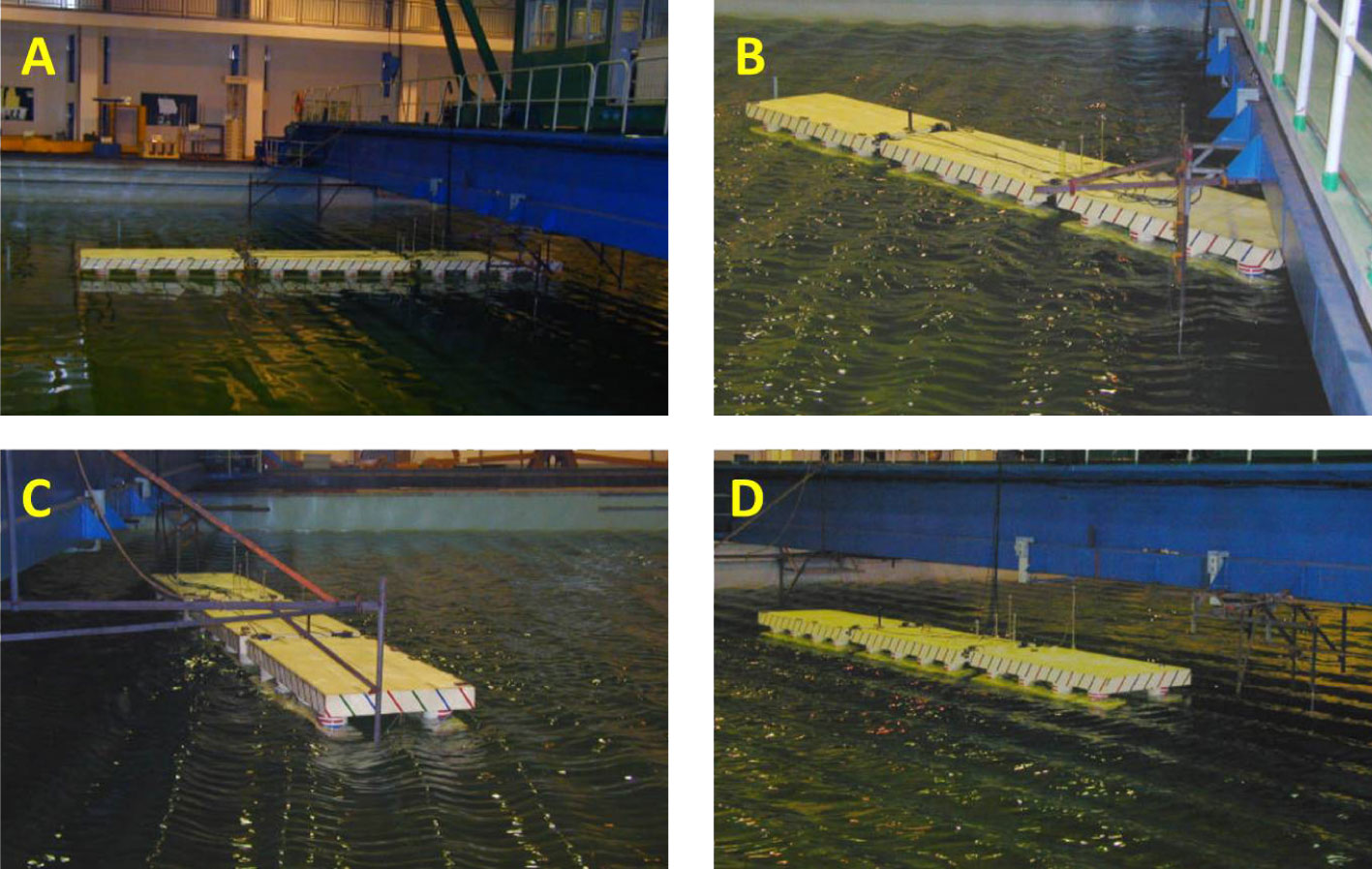
Figure 17 Wave incident directions for CP-VLFS (Ding, 2004 and Yu, 2004): (A) δ = 0°; (B) δ = 45°; (C) δ = 75°; (D) δ = 90°.

During the PFT method in this paper, considering the structural symmetry of CP-VLFS, the single symmetrical composite potential method (SSCPM) was adopted to mesh the elements on the wetted surface for a hydrodynamic numerical model of CP-VLFS with “three modules and four connectors”. The tetrahedron were treated as the element type to constitute and mesh the CP-VLFS model, and a single CP-VLFS module was included 976 elements with total 1024 nodes. The hydrodynamic coefficients, i.e., the added mass, damping coefficient, and static resilience coefficient, and the RIW excitation force on a single module of CP-VLFS in frequency-domain were acquired via using the PFT. Subsequently, the obtained results in frequency-domain were transformed to the time-domain based on the method of fast Fourier transform (FFT) (Wu et al., 2017). According to the aforementioned parameters, the hydrodynamic response results for the CP-VLFS modules were solved in time-domain on the basis of hydrodynamic equation, i.e., Eqs. (35) and (36). Ultimately, the hydrodynamic constraint loads on connectors of CP-VLFS in time-domain were further determined by using the Eqs. (17) and (18).

The wave spectrum of Bretschneider and wave angles (incident wave directions) in the numerical simulation (including this paper’s simplified method and PFT) are set to the same values as in the physical model experiment reported by Ding, 2004 and Yu, 2004. In addition, the shadowing effects of interactions among the columns within CP-VLFS modules for the connector’s time-domain hydrodynamic results of constraint loads are considered in this paper’s rapid and high-efficiency method and the general PFT.

Finally, the maximums (Max), means, significant values (SV), and standard deviations (SD) for hydrodynamic constraint loads of C₁ and C₃ based on the aforementioned three methods, including this paper’s proposed rapid and high-efficiency estimating method, the PFT by this paper, and the experiment reported by literatures (Ding, 2004 and Yu, 2004) are statistically obtained and adopt to compare with each other. Figures 18 and 19 show the contrastive analysis results of the statistical values for hydrodynamic constraint loads of C₁ and C₃ in directions of x, y, and z under different wave angles.

FIGURE 18

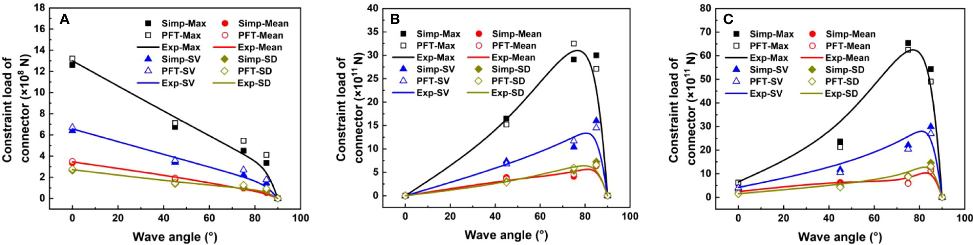
Figure 18 Constraint loads of C₁: (A) x direction; (B) y direction; (C) c direction.

FIGURE 19

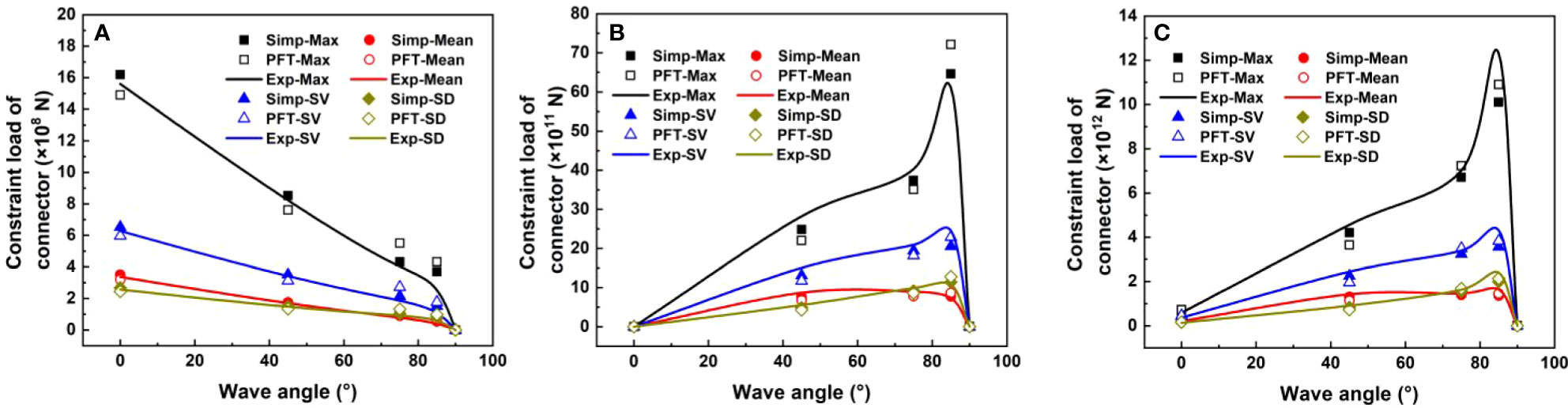
Figure 19 Constraint loads of C₃: (A) x direction; (B) y direction; (C) c direction.

Figures 18 and 19 indicate that:

(1) The statistical results of hydrodynamic constraint loads estimated by this paper’s method for C₁ and C₃ in directions of x, y, and z correspond well with the statistical results of the PFT and the experiment, validating this paper’s methodologies.

(2) The statistical results of hydrodynamic constraint loads for C₁ and C₃ gradually decrease with the wave angles increasing in x direction, and this phenomenon agrees very well with theoretical analysis and practical situation.

(3) Nevertheless, the fluctuation laws between the evaluated values of constraint loads and wave angles show convex in y, and z directions. Especially, the connectors’ constraint loads in directions of y and z present a trend of rapidly decreasing when the wave angles δ>85°.

To quantitatively estimate the differences among this paper’s method and the other two methods (PFT and the experiment), the relative errors of all the statistical constraint loads of C₁ and C₃ are determined under different wave angles. As shown in Figure 20, the relative errors between this paper’s simplified high-efficiency method and PFT, experimental measurements for C₁ and C₃ are all less than 20%, validating the methodologies proposed by this paper.

FIGURE 20

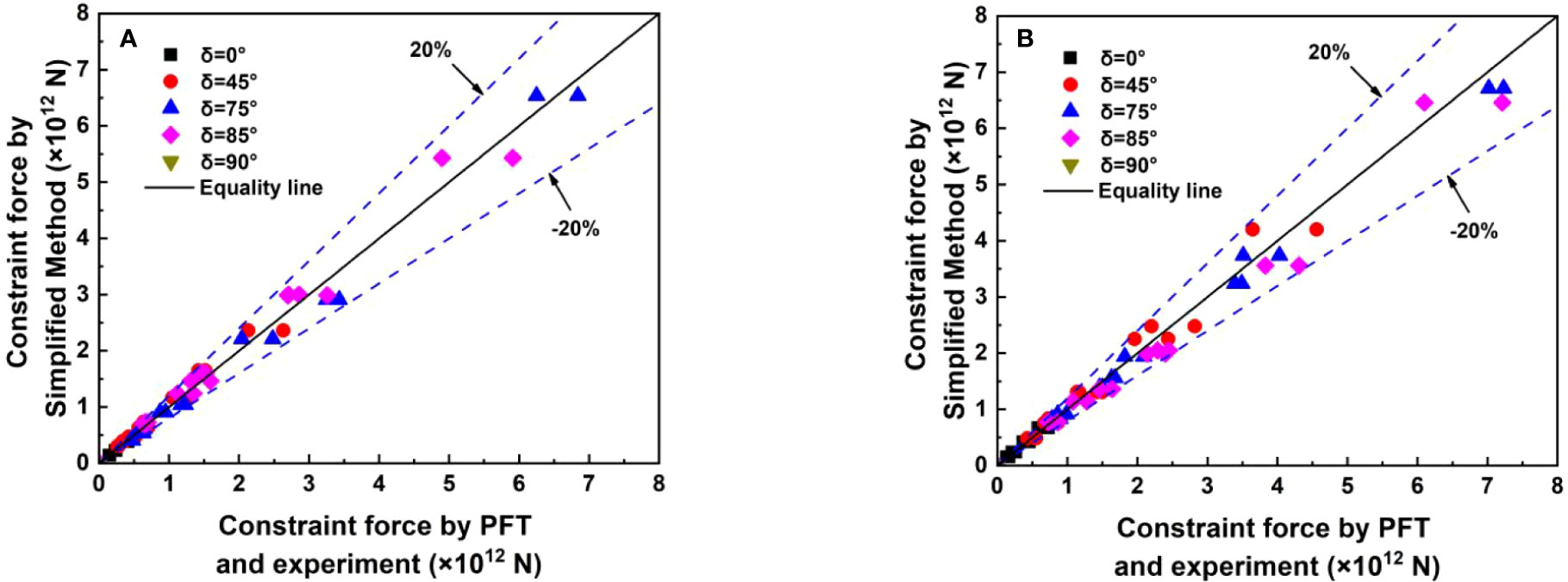
Figure 20 Comparison of the constraint force by simplified method versus those of PFT and experiment: (A) C₁; (B) C₃.

(3) Discussions

In summary, the statistical values of CP-VLFS’s connectors’ hydrodynamic constraint loads estimated by this paper’s method correspond well with the statistical results determined by the PFT and the experiment. Nevertheless, although the data measured from the experiment are more reliable than those from numerical simulations, not all load case combinations of every practical engineering scenario for CP-VLFS can be evaluated by experiments for economical results. Therefore, the development of a rapid, high-efficiency and reasonable method is vital for evaluating the weaknesses of CP-VLFS.

According to the analysis, the main distinctions between the method proposed by this paper and the general PFT are embodied in the theory assessment of wave excitation force. A single CP-VLFS module could be reasonably assumed as an individual semi-submersible platforms. Therefore, the wave forces estimation of CP-VLFS modules largely draws from the relative approaches of semi-submersible platforms (Qiao and Ou, 2013; Fan et al., 2017; Wang et al., 2022b). During the previous studies, the Morison theory of floating body was usually utilized to assess the wave forces on small-scale components, such as the stay bars, within semi-submersible platforms, whereas the wave forces acting on columns and bottom hulls of semi-submersible platforms were confirmed via using the linear diffraction theory (Stansby et al., 2015; Shi Y. et al., 2018; Gabreil et al., 2022) because these components were considered as the large-scale ones comparing with the wave length at general sea states. Wave conditions vary with the increasing water depth in which the platform was located, and the columns and bottom hulls for semi-submersible platforms can be also treated as the small scale-components. Hence, the mode for determining the wave forces of these components by the Morison theory through ignoring interactions between each component was seen as the reasonable (Clauss et al., 2003).

However, for the floating structures of semi-submersible platforms, on which the PFT is still the main method for solving the wave forces. Although the estimation results based on the method of PFT are more accurate, the corresponding theories are relatively complex and would consume plenty of computing time. For instance, the solving time on the basis of the PFT method may last about 2.75 h when the condition of wave angle δ=45°, whereas the computation time for this paper’s rapid and high-efficiency method at a common condition, i.e., δ=45°, only needs 15 min by using a same work computer, while the solving efficiency can be improved more than tenfold. The time-domain hydrodynamic results for CP-VLFS’s connectors on various unfavorable load combinations via adopting the method of PFT during the stage of preliminary design must extremely reduce the solving efficiency. As a result, various significant components for CP-VLFS, including the columns and pontoons, are reasonably assumed as the small-scale components under the HSSs, and the Morison theory of floating body can be utilized to further estimate the wave forces acting on CP-VLFS in this paper. Moreover, the shadowing effects of interactions between front and back columns and modules are considered in this paper’s high-efficiency method. Finally, the hydrodynamic constraint loads for CP-VLFS’s connectors by using this paper’s method are utilized to compare with those of PFT and experiment, as well as the relative errors among the aforementioned three results are quantitatively analyzed. Although the PFT algorithm has a higher computational accuracy, the relative errors of significant values between this paper’s method and PFT are controlled within 20%; therefore, the accuracy, feasibility and reasonability for this paper’s methodology are validated.

This paper’s rapid and high-efficiency method is suitable for estimating the results of time-domain hydrodynamic constraint forces for CP-VLFS’s flexible connectors during the preliminary design stage. it’s worth noting that the preconditions for this paper’s method application are the similar structural style with the CP-VLFSs when exposed to the HSSs, in which the vital components can be regarded as the small-scale components. If not, the Morison theory of floating body cannot be adopted for estimating the marine environmental wave forces acting on structures, such as the VLFS of box type. This feature is the greatest weakness and limitation of this paper’s method.

4 Conclusion

This paper proposed a rapid and high-efficiency method to estimate the time-domain hydrodynamic constraint loads of CP-VLFS’s connectors by the considerations of RMFC model. This solving method is suitable for the structural style of CP-VLFS during the preliminary design stage and at HSSs. The Morison theory of floating body is used to estimate the excitation forces of RIW on CP-VLFSs, and concise formulas for the hydrodynamic constraint loads of CP-VLFS’s connectors are derived on the basis of the geometrical relationship of the CP-VLFS modules’ motion. A numerical model of three-module and four-connectors for CP-VLFS SS6 is considered as a case, and the time-domain hydrodynamic constraint loads of CP-VLFS’s connectors are estimated under the RIWs simulated via the wave spectrum of Bretschneider with different wave angles. The results solving by this paper’s method corresponded well with those of PFT and experiment, validating this paper’s methodologies. In addition, the reasonability of this paper’s method is discussed in details. The findings of this paper can provide significant technical supports for hydrodynamic characteristics for CP-VLFS modules and their connectors optimization.

Data availability statement

The original contributions presented in the study are included in the article/supplementary material. Further inquiries can be directed to the corresponding author.

Author contributions

Conceptualization, methodology: LJW. Writing-original draft preparation, investigation: HJ. Formal analysis, validation: XDJ. Supervision, resources: XLJ. Writing-review & editing: ZYX. Visualization: MJG. All authors have read and agreed to the published version of the manuscript. All authors contributed to the article and approved the submitted version.

Funding

This research is funded by the National Key R&D Program of China (2022YFB3207400), the National Natural Science Foundation of China (52209156), the Science & technology Innovation Project of Chongqing Education Commission (KJCX2020030), the Science Foundation of Chongqing Jiaotong University (F1220025), and the Open-end Fund of Key Laboratory of Hydraulic and Waterway Engineering of the Ministry of Education in Chongqing Jiaotong University (SLK2021B13).

Conflict of interest

The authors declare that the research was conducted in the absence of any commercial or financial relationships that could be construed as a potential conflict of interest.

Publisher’s note

All claims expressed in this article are solely those of the authors and do not necessarily represent those of their affiliated organizations, or those of the publisher, the editors and the reviewers. Any product that may be evaluated in this article, or claim that may be made by its manufacturer, is not guaranteed or endorsed by the publisher.

References

Bonakdar L., Oumeraci H. (2015). Pile group effect on the wave loading of a slender pile: A small-scale model study. Ocean Eng. 108, 449–461. doi: 10.1016/j.oceaneng.2015.08.021

CrossRef Full Text | Google Scholar

Clauss G. F., Schmittner C. E., Stutz K. (2003). Freak wave impact on semisubmersibles-time-domain analysis of motions and forces, in Proceedings of 13th International Offshore and Polar Engineering Conference (ISOPE-2003), Honolulu, USA, Vol. 13. 449–456.

Google Scholar

Ding W. (2004). Experimental research on mobile offshore base (Master’s thesis) (Shanghai: Shanghai Jiaotong University).

Google Scholar

Ding R., Liu C. R., Zhang H. C., Xu D. L., Shi Q. J., Yan D. L., et al. (2020). Experimental investigation on characteristic change of a scale-extendable chain-type floating structure. Ocean Eng. 213, 107778. doi: 10.1016/j.oceaneng.2020.107778

CrossRef Full Text | Google Scholar

Ding J., Tian C., Wu Y. S., Li Z. W., Ling H. J., Ma X. Z. (2017). Hydroelastic analysis and model tests of a single module VLFS deployed near islands and reefs. Ocean Eng. 144, 224–234. doi: 10.1016/j.oceaneng.2017.08.043

CrossRef Full Text | Google Scholar

Ding J., Tian C., Wu Y. S., Wang X. F., Liu X. L., Zhang K. (2019). A simplified method to estimate the hydroelastic responses of VLFS in the inhomogeneous waves. Ocean Eng. 172, 434–445. doi: 10.1016/j.oceaneng.2018.12.025

CrossRef Full Text | Google Scholar

Ding J., Wu Y. S., Zhou Y., Ma X. Z., Ling H. J., Xie Z. Y. (2020b). Investigation of connector loads of a 3-module VLFS using experimental and numerical methods. Ocean Eng. 195, 106684. doi: 10.1016/j.oceaneng.2019.106684

CrossRef Full Text | Google Scholar

Ding J., Xie Z. Y., Wu Y. S., Xu S. W., Qiu G. Y., Wang Y. T., et al. (2020a). Numerical and experimental investigation on hydroelastic responses of an 8-module VLFS near a typical island. Ocean Eng. 214, 107841. doi: 10.1016/j.oceaneng.2020.107841

CrossRef Full Text | Google Scholar

Ding W., Yu L., Li R. P., Yao M. W. (2005). Experimental research on dynamic responses of mobile offshore base connector. Ocean Eng. 23 (2), 11–15. doi: 10.16483/j.issn.1005-9865.2005.02.002

CrossRef Full Text | Google Scholar

Drummen I., Olbert G. (2021). Conceptual design of a modular floating multi-purpose island. Front. Mar. Sci. 8. doi: 10.3389/fmars.2021.615222

CrossRef Full Text | Google Scholar

Fan T. H., Qiao D. S., Yan J., Chen C. H., Ou J. P. (2017). Experimental verification of a semi-submersible platform with truncated mooring system based on static and damping equivalence. Ships Offshore Struc. 12 (8), 1145–1153. doi: 10.1080/17445302.2017.1319542

CrossRef Full Text | Google Scholar

Flikkema M., Waals O. (2019). Space@Sea the floating solution. Front. Mar. Sci. 6. doi: 10.3389/fmars.2019.00553

CrossRef Full Text | Google Scholar

Gabreil E., Wu H. T., Chen C., Li J. Y., Rubinato M., Zheng X., et al. (2022). Three-dimensional smoothed particle hydrodynamics modeling of near-shore current flows over rough topographic surface. Front. Mar. Sci. 9. doi: 10.3389/fmars.2022.935098

PubMed Abstract | CrossRef Full Text | Google Scholar

Gao R. P., Tay Z. Y., Wang C. M., Koh C. G. (2011). Hydroelastic response of very large floating structure with a flexible line connection. Ocean Eng. 38 (17-18), 1957–1966. doi: 10.1016/j.oceaneng.2011.09.021

CrossRef Full Text | Google Scholar

Kim J., Cho S., Kim K., Lee P. (2014). Hydroelastic design contour for the preliminary design of very large floating structures. Ocean Eng. 78, 112–123. doi: 10.1016/j.oceaneng.2013.11.006

CrossRef Full Text | Google Scholar

Lamas-Pardo M., Iglesias G., Carral L. (2015). A review of very large floating structures (VLFS) for coastal and offshore uses. Ocean Eng. 109, 677–690. doi: 10.1016/j.oceaneng.2015.09.012

CrossRef Full Text | Google Scholar

Li Q. M., Wu L. J., Wang Y. Z., Li Y. (2017). Hydrodynamic coefficients of semi-submersible type very large floating structures. Ocean Eng. 1, 1–11. doi: 10.16483/j.issn.1005-9865.2017.01.001

CrossRef Full Text | Google Scholar

Lian Y. S., Yim S. C., Zheng J. H., Liu H. X., Zhang N. (2020). Effects of damaged fiber ropes on the performance of a hybrid taut-wire mooring system. J. Offshore Mech. Arct. Eng. 142 (1), 011607. doi: 10.1115/1.4044723

CrossRef Full Text | Google Scholar

Liu O. R., Molina R. (2021). The persistent transboundary problem in marine natural resource management. Front. Mar. Sci. 8. doi: 10.3389/fmars.2021.656023

CrossRef Full Text | Google Scholar

Nie W., Liu Y. Q. (2002). Structural dynamic analysis in ocean engineering (Harbin Engineering University Press) 50–90.

Google Scholar

Qi T., Huang X. P., Li L. B. (2018). Spectral-based fatigue crack propagation prediction for very large floating structures. Mar. Struct. 57, 193–206. doi: 10.1016/j.marstruc.2017.10.003

CrossRef Full Text | Google Scholar

Qiao D. S., Feng C. L., Ning D. Z., Wang C., Liang H. Z., Li B. B. (2020). Dynamic response analysis of jacket platform integrated with oscillating water column device. Front. Energy Res. 8. doi: 10.3389/fenrg.2020.00042

PubMed Abstract | CrossRef Full Text | Google Scholar

Qiao D. S., Mackay E., Yan J., Feng C. L., Li B. B., Feichtner A., et al. (2021). Numerical simulation with a macroscopic CFD method and experimental analysis of wave interaction with fixed porous cylinder structures. Mar. Struct. 80, 103096. doi: 10.1016/j.marstruc.2021.103096

CrossRef Full Text | Google Scholar

Qiao D. S., Ou J. P. (2013). Global responses analysis of a semi-submersible platform with different mooring models in south China Sea. Ships Offshore Struct. 8 (5), 441–456. doi: 10.1080/17445302.2012.718971

CrossRef Full Text | Google Scholar

Rayner R., Jolly C., Gouldman C. (2019). Ocean observing and the blue economy. Front. Mar. Sci. 6. doi: 10.3389/fmars.2019.00330

CrossRef Full Text | Google Scholar

Ren N. X., Zhang C., Magee A. R., Hellan Ø., Dai J., Ang K. K. (2019). Hydrodynamic analysis of a modular multi-purpose floating structure system with different outermost connector types. Ocean Eng. 176, 158–168. doi: 10.1016/j.oceaneng.2019.02.052

CrossRef Full Text | Google Scholar

Shi Y., Li S. W., Chen H. B., He M., Shao S. D. (2018). Improved SPH simulation of spilled oil contained by flexible floating boom under wave–current coupling condition. J. Fluid Struct. 76, 272–300. doi: 10.1016/j.jfluidstructs.2017.09.014

CrossRef Full Text | Google Scholar

Shi Q. J., Xu D. L., Zhang H. C., Zhao H., Wu Y. S. (2018). Optimized stiffness combination of a flexible-base hinged connector for very large floating structures. Mar. Struc. 60, 151–164. doi: 10.1016/j.marstruc.2018.03.014

CrossRef Full Text | Google Scholar

Singla S., Martha S., Sahoo T. (2018). Mitigation of structural responses of a very large floating structure in the presence of vertical porous barrier. Ocean Eng. 165, 505–527. doi: 10.1016/j.oceaneng.2018.07.045

CrossRef Full Text | Google Scholar

Souravlias D., Dafnomilis I., Ley J., Assbrock G., Duinkerken M. B., Negenborn R. R., et al. (2020). Design framework for a modular floating container terminal. Front. Mar. Sci. 7. doi: 10.3389/fmars.2020.545637

CrossRef Full Text | Google Scholar

Stansby P., Moreno E. C., Stallard T., Maggi A. (2015). Three-float broad-band resonant line absorber with surge for wave energy conversion. Renew. Energ. 78, 132–140. doi: 10.1016/j.renene.2014.12.057

CrossRef Full Text | Google Scholar

Wang Z. M., Qiao D. S., Tang G. Q., Wang B., Yan J., Ou J. P. (2022a). An identification method of floating wind turbine tower responses using deep learning technology in the monitoring system. Ocean Eng. 261, 112105. doi: 10.1016/j.oceaneng.2022.112105

CrossRef Full Text | Google Scholar

Wang Z. M., Qiao D. S., Yan J., Tang G. Q., Li B. B., Ning D. Z. (2022b). A new approach to predict dynamic mooring tension using LSTM neural network based on responses of floating structure. Ocean Eng. 249, 110905. doi: 10.1016/j.oceaneng.2022.110905

CrossRef Full Text | Google Scholar

Wang C. M., Tay Z. Y. (2011). Very large floating structures: applications, research and development. Proc. Eng. 14, 62–72. doi: 10.1016/j.proeng.2011.07.007

CrossRef Full Text | Google Scholar

Wei W., Fu S. X., Moan T., Lu Z. Q., Deng S. (2017). A discrete-modules-based frequency domain hydroelasticity method for floating structures in inhomogeneous sea conditions. J. Fluid. Struc. 74, 321–339. doi: 10.1016/j.jfluidstructs.2017.06.002

CrossRef Full Text | Google Scholar

Wei W., Fu S. X., Moan T., Song C. H., Ren T. X. (2018). A time-domain method for hydroelasticity of very large floating structures in inhomogeneous sea conditions. Mar. Struct. 57, 180–192. doi: 10.1016/j.marstruc.2017.10.008

CrossRef Full Text | Google Scholar

Wu L. J., Wang Y. Z., Li Q. M., Li Y. (2016b). Simplified computational method for wave force of semi-submersible very large floating structures based on floating body morison equation. Ship Eng. 38 (12), 56–62. doi: 10.13788/j.cnki.cbgc.2016.12.056

CrossRef Full Text | Google Scholar

Wu L. J., Wang Y. Z., Li Y., Xiao Z., Li Q. M. (2017). Simplified algorithm for evaluating the hydrodynamic performance of very large modular semi-submersible structures. Ocean Eng. 140, 105–124. doi: 10.1016/j.oceaneng.2017.05.013

CrossRef Full Text | Google Scholar

Wu L. J., Wang Y. Z., Wang Y. C., Chen J. Y., Li Y., Li Q. M., et al. (2018). Optimal stiffness for flexible connectors on a mobile offshore base at rough Sea states. China Ocean Eng. 32 (6), 683–695. doi: 10.1007/s13344-018-0070-5

CrossRef Full Text | Google Scholar

Wu L. J., Wang Y. Z., Xiao Z., Li Y. (2016a). Hydrodynamic response for flexible connectors of mobile offshore base at rough sea states. Petrol. Explor. Dev. 43 (6), 1089–1096. doi: 10.11698/PED.2016.06.18

CrossRef Full Text | Google Scholar

Xiao L. F., Kou Y. F., Tao L. B., Yang L. J. (2016). Comparative study of hydrodynamic performances of breakwaters with double-layered perforated walls attached to ring-shaped very large floating structures. Ocean Eng. 111, 279–291. doi: 10.1016/j.oceaneng.2015.11.007

CrossRef Full Text | Google Scholar

Xu X. S., Xing Y. H., Gaidai O., Wang K. L., Patel K. S., Dou P., et al. (2022). A novel multi-dimensional reliability approach for floating wind turbines under power production conditions. Front. Mar. Sci. 9. doi: 10.3389/fmars.2022.970081

PubMed Abstract | CrossRef Full Text | Google Scholar

Yang P., Liu X. L., Wang Z. D., Zong Z., Tian C., Wu Y. S. (2019). Hydroelastic responses of a 3-module VLFS in the waves influenced by complicated geographic environment. Ocean Eng. 184, 121–133. doi: 10.1016/j.oceaneng.2019.05.020

CrossRef Full Text | Google Scholar

Yao W. J., Shi Y. S. (2022). Dynamic stability analysis of pile groups under wave load. Appl. Math. Model. 110, 367–386. doi: 10.1016/j.apm.2022.06.003

CrossRef Full Text | Google Scholar

Yu L. (2004). Study on dynamic responses of connectors of mobile offshore base (Doctoral thesis) (Shanghai: Shanghai Jiaotong University).

Google Scholar

Zhang B., Qi E. R., Lu Y., Yi Q., Liu C. (2013). Influence of module number on dynamic responses of very large mobile offshore base. Ship Mech. 17 (Z1), 49–55. doi: 10.3969/j.issn.1007-7294.2013.h1.007

CrossRef Full Text | Google Scholar

Zhao H., Xu D. L., Zhang H. C., Xia S. Y., Shi Q. J., Ding R., et al. (2019). An optimization method for stiffness configuration of flexible connectors for multi-modular floating systems. Ocean Eng. 181, 134–144. doi: 10.1016/j.oceaneng.2019.03.039

CrossRef Full Text | Google Scholar

Zhao W. H., Yang J. M., Hu Z. Q., Tao L. B. (2014a). Coupled analysis of nonlinear sloshing and ship motions. Appl. Ocean Res. 47, 85–97. doi: 10.1016/j.apor.2014.04.001

CrossRef Full Text | Google Scholar

Zhao W. H., Yang J. M., Hu Z. Q., Xiao L. F., Tao L. B. (2014b). Hydrodynamics of a 2D vessel including internal sloshing flows. Ocean Eng. 84, 45–53. doi: 10.1016/j.oceaneng.2014.03.001

CrossRef Full Text | Google Scholar