Deriving pre-eutrophic conditions from an ensemble model approach for the North-West European seas

1 Introduction

Nutrient inputs into the marine environment predominantly come from riverine inputs, direct discharges and atmospheric deposition. Elevated nutrient concentrations may lead to undesirable increases in primary production, and subsequent degradation of the sinking organic matter can lead to oxygen deficits near the seafloor (Diaz and Rosenberg, 2008; Greenwood et al., 2010; Große et al., 2016). This process, called eutrophication, is related to an increase in nutrient loads from anthropogenic sources (Jickells, 1998; Nixon, 2009). Additional symptoms of marine eutrophication include harmful algae blooms (Schoemann et al., 2005; Riegman et al., 1992) and loss of seagrasses (Burkholder et al., 2007), resulting in qualitative changes in the local marine food web. The smelly foam on beaches left in the wake of Phaeocystis blooms are well known to the general public and tourist’s industries, but toxins released by some algae blooms also directly threaten human economic interests and human life, usually via (consumption of) affected marine resources (Berdalet et al., 2016).

Eutrophication effects became increasingly evident in the North Sea around 1980, and it was broadly recognized that this phenomenon was related to anthropogenic sources. The regional sea convention for the North-East Atlantic OSPAR (www.ospar.org) defined eutrophication as “the enrichment of water by nutrients causing an accelerated growth of algae and higher forms of plant life to produce an undesirable disturbance to the balance of organisms present in the water and to the quality of the water concerned, and therefore refers to the undesirable effects resulting from anthropogenic enrichment by nutrients” (OSPAR, 1998, p. 53), confirming the cause-effect relationship with anthropogenic sources. Following the early evidence of eutrophication, OSPAR applied a source-oriented approach since 1988, through limiting inputs of nutrients and organic matter to levels that do not give rise to adverse effects on the marine environment. The proposed reduction was very successful for phosphorus (which is caused mainly by point-sources, e.g. sewage) but less so for nitrogen (caused mainly by diffuse sources, e.g. agriculture) (Claussen et al., 2009; Conley et al., 2009). As a result, though eutrophication effects have declined since their 1980’s peak, they are even now persistent in many western European coastal areas. The latest application of OSPAR’s Common Procedure (COMP3, OSPAR, 2017) still identified large parts of the southern North Sea along the Belgian, Dutch, German and Danish coasts as so-called “problem areas” or “potential problem areas” with respect to eutrophication, with smaller areas along the French and British coasts also characterized as such. The Kattegat was also defined as a “problem area”, as were smaller parts along the Swedish and Norwegian coasts.

Recovery from a eutrophic state can be a lengthy process (~ decades, McCrackin et al., 2017), and does not always lead to the ecological state observed before eutrophication occurred (Duarte et al., 2008; Oguz and Velikova, 2010). It is therefore critical to establish appropriate restoration goals for eutrophied areas (McCrackin et al., 2017). The objective of the presented work is to quantify the pre-eutrophic state of the Northwest European Shelf, based on an ecosystem modelling ensemble approach applied by OSPAR’s ICG-EMO (Intersessional Correspondence Group on Ecosystem Modelling). Here the pre-eutrophic state is defined as the situation around the year 1900, and is by no means a pristine or anthropogenically undisturbed state. To account for regional differences in performance between the models, the ensemble mean applies a weighting method (Almroth & Skogen, 2010) based on the level of agreement between current model simulations and current observations. These weights are then applied to construct the ensemble-simulated pre-eutrophic state, thus providing a sophisticated estimate of the mean pre-eutrophic concentrations, which can serve as baseline for eutrophication assessments. This paper presents the harmonized modelling approach, the applied ensemble weighting method, the underlying assumptions, as well as the resulting estimates of pre-eutrophic nutrient and phytoplankton concentrations. These values can support the elaboration of policy thresholds for eutrophication that are coherent across national boundaries. We demonstrate that an ensemble modelling approach can help to define pre-eutrophic values for indicators of eutrophication across vast marine regions, while keeping a focus on local ecosystem functioning and on the continuity of transboundary processes.

2 Methods

2.1 Ensemble method overview

Eight modelling centres participated in the ensemble modelling exercise. To ensure comparable results between the different models in the ensemble, some harmonized model inputs were prescribed in a joint protocol. These included all external sources of nutrients: riverine nutrient loads, atmospheric deposition and boundary conditions. S imulation period and model output variables were also prescribed. Meteorological forcing was not prescribed, to allow the participants to use the same forcings as applied in published validation results. Each partner also used its standard bathymetry, for the same reason. Boundary conditions were taken from a shared source. All partners were asked to submit results for 2009-2014 (the COMP3 assessment period) for variables aligned with the eutrophication assessment protocol by OSPAR: Dissolved Inorganic Nitrogen (DIN, surface layer), Dissolved Inorganic Phosphorus (DIP, surface layer), Total Nitrogen (TN, depth-averaged), Total Phosphorous (TP, depth-averaged) and the nitrogen to phosphorus (N:P, depth-averaged) ratio for the winter period (December-February). Chlorophyll (Chl, surface layer), chlorophyll 90^th percentile (Chl P90, surface layer) and light attenuation (K_d, surface layer) were averaged over the growing season (March-September), while near-bed oxygen levels (O₂, near-bed layer) and net primary production (netPP, depth-integrated) were considered over the whole year. Models with no benthic compartment applied a three-year spin up period to move from initial conditions. Models with a benthic compartment capable of nutrient storage applied a longer, suitable spin up period for the historic scenario to arrive at an equilibrium between benthic nutrients and the applied nutrient inputs.

The participating modelling centres were: the Cefas (Centre for Fisheries and Aquaculture Science, Lowestoft, UK), Deltares (Netherlands), IFREMER (L’Institut Français de Recherche pour l’Exploitation de la Mer, France), JRC (Joint Research Centre in Ispra, Italy but representing the EU), the University of Oldenburg (Oldenburg, Germany), RBINS (Royal Belgian Institute of Natural Sciences, Belgium), SMHI (Swedish Meteorological and Hydrological Institute, Sweden), and the University of Hamburg together with the Helmholtz Zentrum Geesthacht (now called Hereon) (UHH-HZG, Germany). A detailed overview of the different models is provided in Appendix D (descriptions, Supplementary Materials) and E (table overview, Supplementary Materials). Both large domain models (covering the entire Northwest European shelf) and small domain models (covering e.g. only the English Channel or the Southern North Sea) were applied to the exercise.

The different models have varying degrees of complexity with respect to the processes they represent. Not all use the same external nutrient inputs (Table 1) or have the same number of plankton functional groups (Appendix E; Supplementary Table 2). Besides internal model differences the simulations used in this exercise also differ in spatial resolution (Appendix E; Supplementary Table 2) and coverage (Figure 1). Only the SMHI model domain includes the full Baltic Sea, all other domains have an open boundary with the Baltic in the Belt Sea region. Table 1 shows the nutrients that are used as inputs in the different models. Note that even if a model does not use input for a certain nutrient, the dynamics of this nutrient are usually still part of the model’s internal dynamics (Appendix E; Supplementary Table 2).

TABLE 1

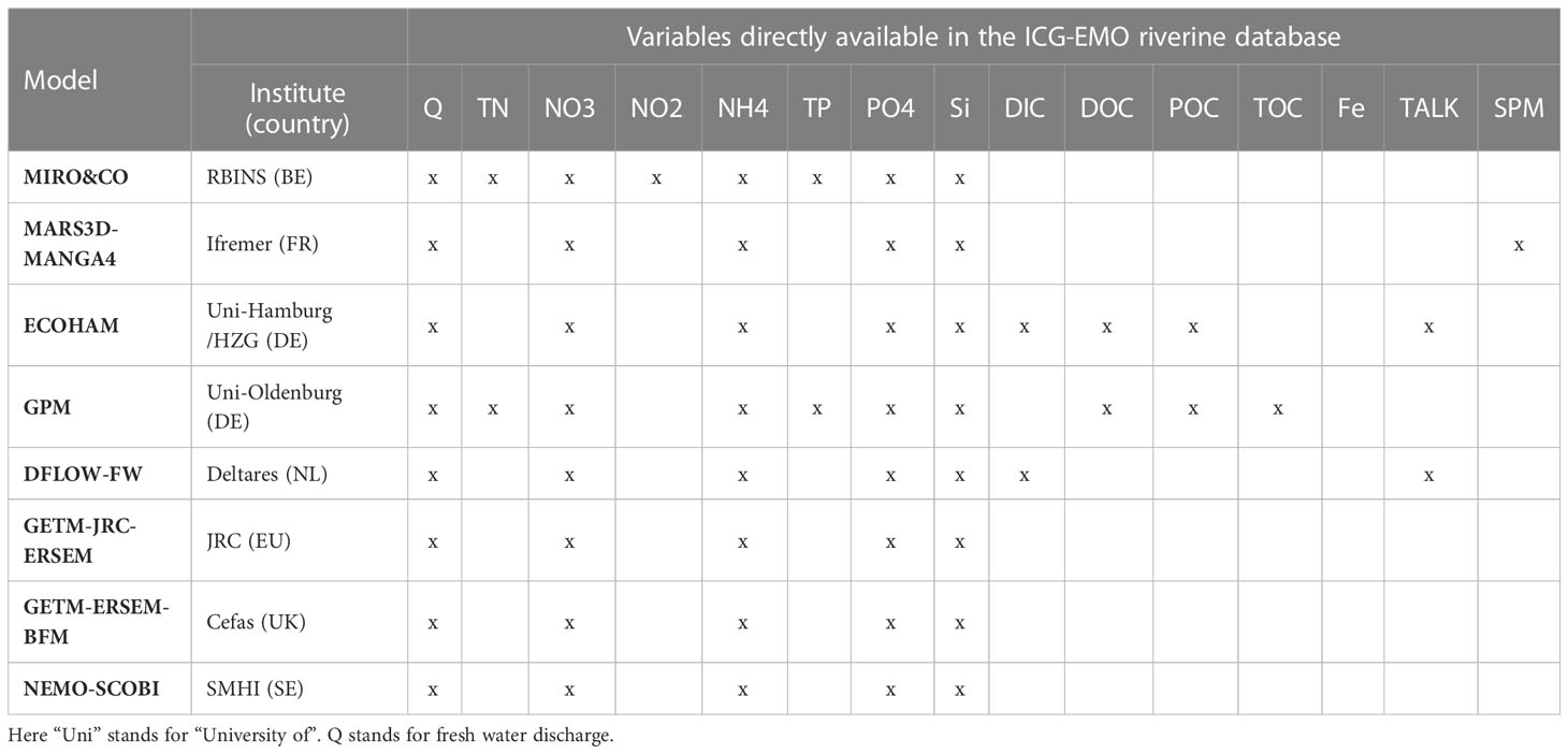
Table 1 Overview of the nutrients used by each model from the supplied riverine input.

FIGURE 1

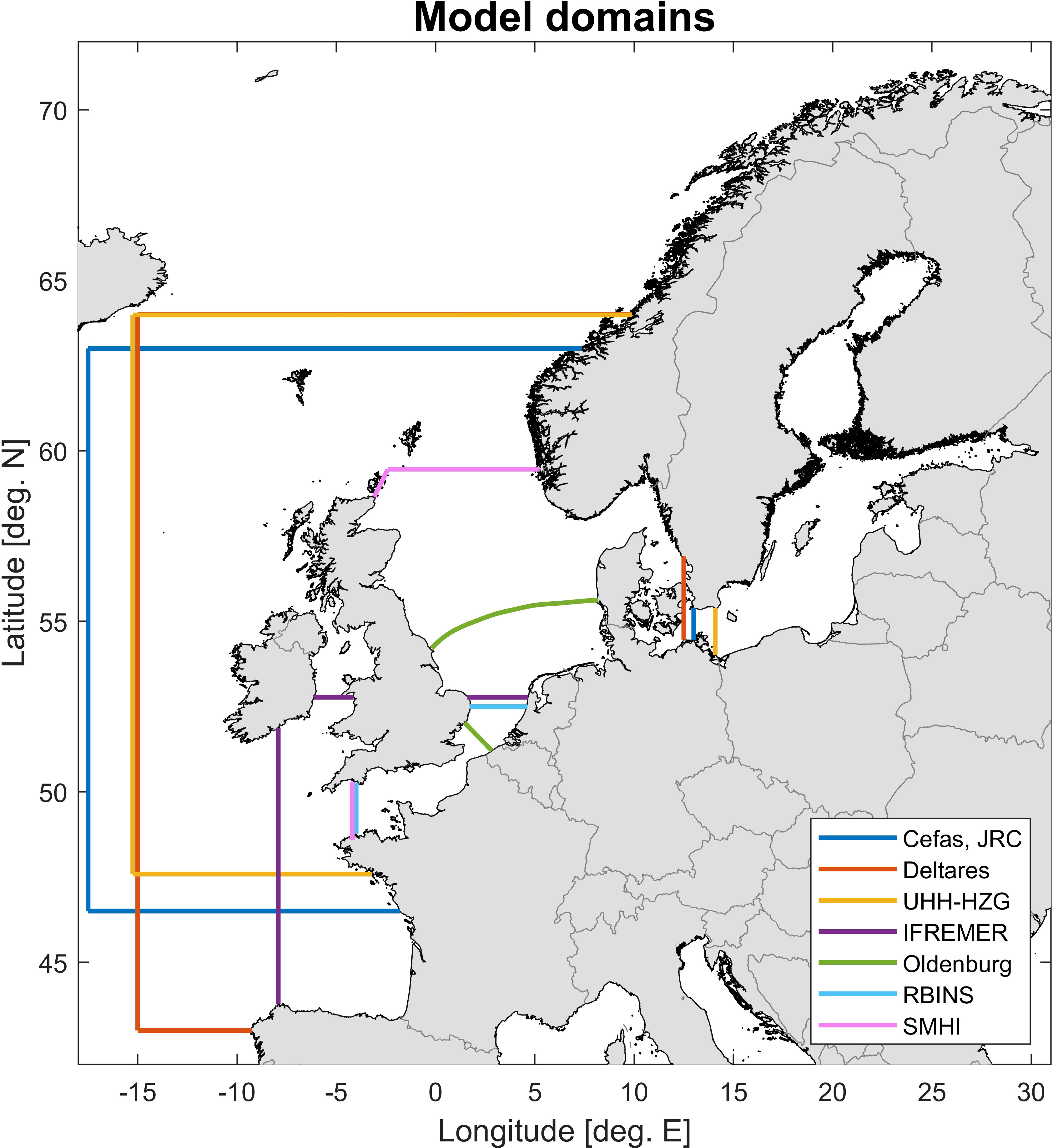
Figure 1 Model domains of the different models used to calculate pre-eutrophic marine conditions. Note that the JRC (Joint Research Centre, EU) and Cefas model domains are identical, though their ecosystem models are different.

2.2 Available observational data

Observations were obtained from the OSPAR Common Procedure Eutrophication Assessment Tool (COMPEAT, see GitHub - ices-tools-prod/COMPEAT, ICES, 2022) for validation and weighting purposes. This tool is applied in the OSPAR Comprehensive Procedure (COMP) for the determination of the eutrophication status of marine areas based on observational data submitted by each member country. The observations, which are the same as those used in the official eutrophication assessments, have a higher spatial and temporal coverage in coastal areas than in offshore waters (see Appendix B; Supplementary Materials). Thus, spatial averages of the observations over assessment areas that comprise coastal and more open waters may not be fully representative of these assessment areas. Simulated area-averaged results will always be representative of the full area, complicating a direct comparison with the observational averages (see, e.g., Garcia-Garcia et al., 2019). Observations were available for DIN, DIP and Chl. Due to the low confidence in the in-situ Chl observations (Appendix B; Supplementary Figure 3) related to data scarcity (both temporally and spatially), satellite data (a reanalysis product, Van der Zande et al., 2019; Lavigne et al., 2021) were added to the Chl observational database in COMPEAT. To calculate a combined seasonal mean concentration per assessment area from in-situ and Earth Observation (EO) data a weighting factor was applied, based on the OSPAR confidence rating of in-situ data availability which is implemented in the COMPEAT tool. Where the combined temporal and spatial confidence of in-situ Chl was high, 50:50 (in-situ/EO) data was used to derive the assessment area mean. If in-situ confidence was moderate, 30:70 (in-situ/EO) was used, while where in-situ confidence was low, 10:90 (in-situ/EO) was applied (OSPAR, 2022a). Coastal waters are optically challenging environments for satellite wavelength observations, due to shallow depths and high levels of suspended matter. Retrieving accurate Chl estimates from satellite data is therefore more challenging in coastal waters than in offshore waters (Lavigne et al., 2021).

Observational time series were extracted for the stations with the most complete temporal coverage over the simulated period (available in the ICES COMPEAT tool), for validation purposes. Unfortunately, using these data results in a strong spatial bias, as most observations were obtained in near-shore waters of the southern North Sea. In addition, data from long-term observation stations were provided by Cefas (station Stonehaven) and PML (station WCO-L4). See Supplementary Figure 2 in the supplementary materials for the locations of the used stations.

2.3 Model validation

Each model used in this exercise has been validated separately before this application (see Supplementary Materials Appendix D). A common validation procedure was applied using a subsection of the COMPEAT data, representing short-term and long-term time series, augmented with 2 additional long-term stations (Stonehaven, WCO-L4) to allow for a comparison of model performance (Figure 2).

FIGURE 2

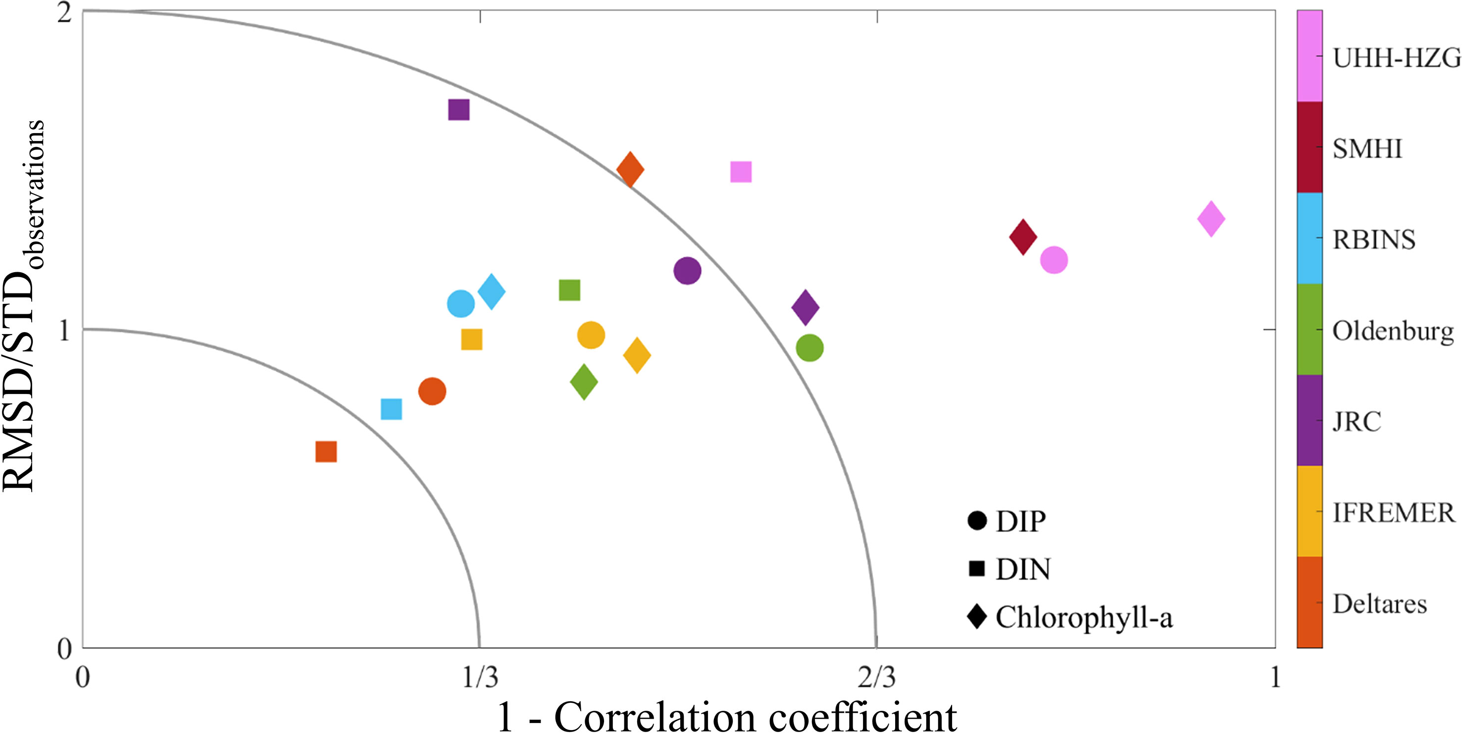
Figure 2 Model skill assessment for DIN, DIP and Chl for all participating models (in respective areas where the number of observations is the highest). The horizontal axis shows 1 - the correlation coefficient between model values and observations, the vertical axis shows the root mean square difference (RMSD) divided by the observational standard deviation (STD). The closer the values are to the origin, the closer the model results are to observations. The inner field (x-axis: 0–1/3, y-axis: 0—1) indicates good agreement and strong correlation between model and observations. The middle field (x-axis: 1/3–2/3, y-axis: 1–2) indicates reasonable agreement and moderate correlation between model and observations. The outer field indicates poor agreement between model and observations. SMHI values for DIN and DIP are off the scale at (0.35, 3.61) and (0.32,3.42), respectively. Negative correlations did not occur.

Following the approach of Eilola et al. (2011) and Edman and Omstedt (2013), we used a combination of correlation coefficient and the root mean square difference (RMSD) scaled by the standard deviation of the observations to assess the skills of the different ecosystem models compared to the observations. This comparison was done for each station individually and later the station results were combined to assess the overall skill for each model (Figure 2). Overall, most model systems have a good to acceptable model skill. Two model systems (JRC and SMHI) were suffering from quite high RMSD values, although these were mostly caused by just a few areas (mainly small estuarine/coastal areas with high inputs and insufficient spatial resolution in the models).

2.4 Assessment areas

As models differed in their spatial resolution and domain coverage, evaluation and comparison to observations were applied per area. Here, we use the areas as defined by OSPAR for use in the 4^th application of the Common procedure (COMP4, Enserink et al., 2019; OSPAR, 2022b). The areas are based on the eco-hydrodynamic regimes as defined by van Leeuwen et al. (2015), refined in the JMP-EUNOSAT project (Enserink et al., 2019) and by the OSPAR contracting parties (OSPAR, 2022a). The area delineation is given in Appendix C, and can be seen in Figure 3. Model results were included in the ensemble mean for an assessment area if the model domain covered 80% or more of the area. As a result, different assessment areas were covered by different numbers of models (Figure 3). For two areas model results have been included despite insufficient domain coverage: the Atlantic area (ATL, UHH-HZG 59.5% coverage) and the Northern North Sea area (NNS, SMHI 78% coverage). The areas included for the individual models are visible in Supplementary Figures 5-7 in Appendix F. Areas with the highest model coverage are the river plumes in the Southern Bight of the North Sea (Scheldt plume 1 and 2, Meuse plume, Rhine plume, inset) and those in the northern part of the English Channel. Maximum number of models contributing is 7, as Cefas was unable to provide results for the pre-eutrophic scenario due to technical issues. However, Cefas did contribute to the harmonization effort, observational data gathering, the applied approach, negotiations and overall methodology. Therefore their submitted current state results are included in Appendix F, but are not included in the presented analysis.

FIGURE 3

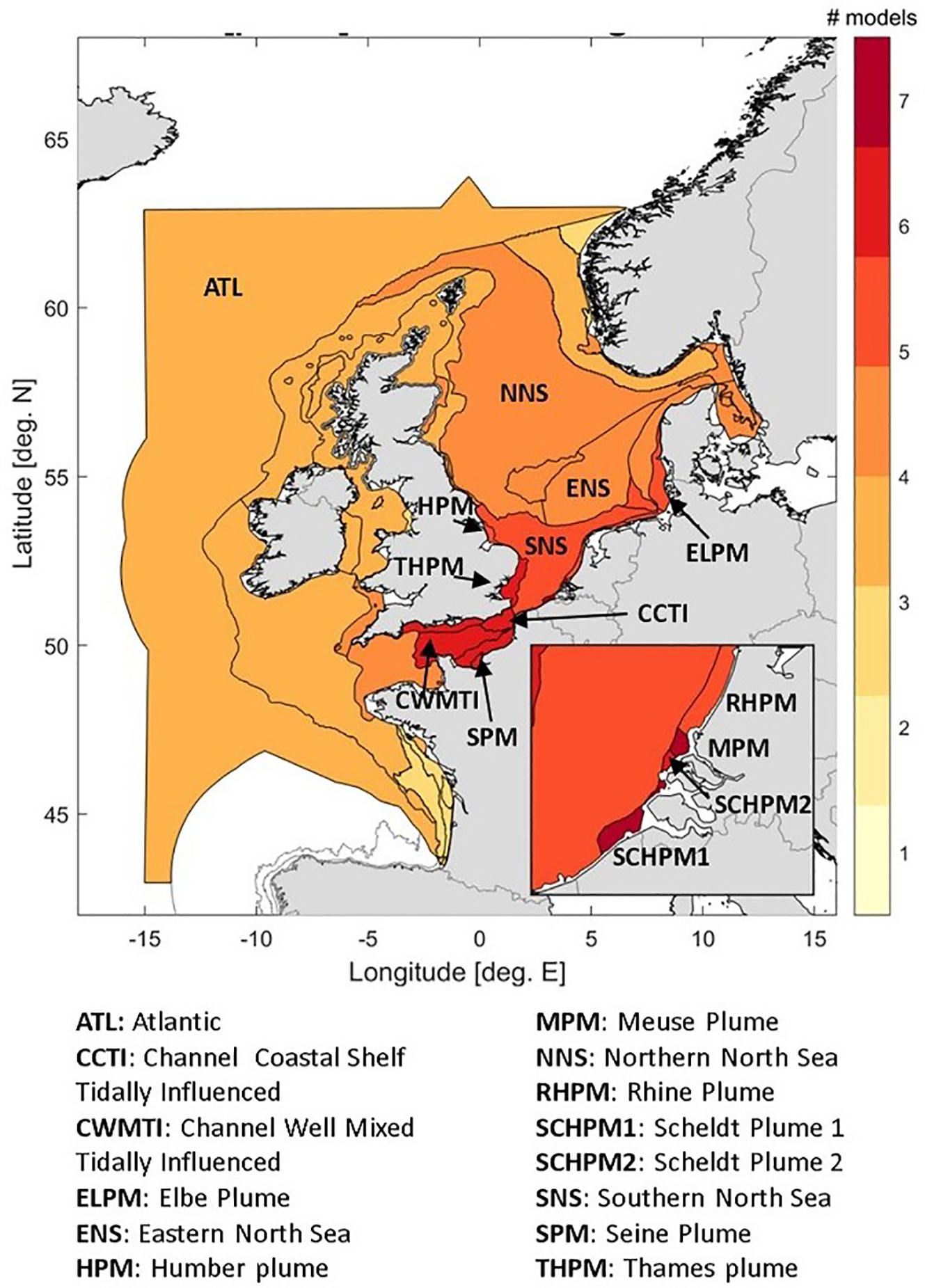
Figure 3 Number of models per assessment area, that have been included in the calculation of area means.

2.5 Current state scenario

The current state scenario (hereafter, CS) applied the ICG-EMO database of European rivers for the riverine nutrient inputs of the selected period. This database contains daily values for flow and nutrients for 368 rivers discharging onto the European Shelf, following optimization to daily values from originally sourced observational data (Lenhart et al., 2010; ICG-EMO, 2021). For an overview of the rivers included see Appendix A (Supplementary Materials). The average atmospheric deposition rates for NO_x, NH₃ and Total Nitrogen over the North Western Continental Shelf as estimated by EMEP (EMEP, 2020) were used for atmospheric input of nutrients, with values provided in Table 2.

TABLE 2

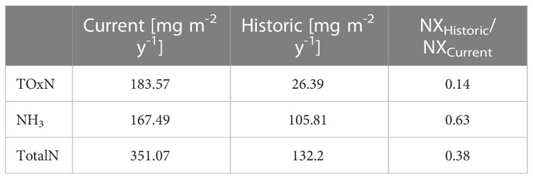
Table 2 Average N deposition rates for the current (2009-2014) and historic (1890-1900) time periods over the North Western Continental Shelf and the respective ratios (Schöpp et al., 2003).

For the open sea boundaries, information from CMEMS (Copernicus Marine Service, EU, https://marine.copernicus.eu/) was used: NORTHWESTSHELF_REANALYSIS_PHY_004_009 (https://doi.org/10.48670/moi-00059) for the physical requirements and NORTHWESTSHELF_REANALYSIS_BIO_004_011 (https://doi.org/10.48670/moi-00058) (Ciavatta et al., 2018) for the chemical and biological state variables (both 0.067 x 0.111 degree spatial resolution with 24 depth levels). The exchange between the Baltic Sea and North Sea in the Kattegat and Skagerrak area is very complex (deep stratified waters, different layers flowing in different directions). To simplify the inflow of nutrient-rich Baltic waters into the North Sea the boundaries of the participating models were selected to be at two shallow sills where flow patterns are less complicated: Darss sill and Drogden sill. Estimates from simulated Baltic Sea discharges by DHI for recent years provided monthly mean climatologies for the water flows at the two sills. For nutrient concentrations recent observations (2009 – 2014) near the sills were used to provide monthly mean climatologies (flow and nutrients: Stiig Markager, pers. comm.). For silicate, an annual mean estimate of 10.4 µM was used (Mantikci, 2014).

2.6 Pre-eutrophic scenario

The pre-eutrophic or historical scenario (hereafter, HS) should reflect the state of European Shelf marine waters before major anthropogenic nutrient inputs occurred. Here, we follow the definition of the project Joint Monitoring Programme of the Eutrophication of the North Sea with Satellite data (JMP-EUNOSAT, Enserink et al., 2019) which uses a period around the year 1900 during the European industrialization but before agricultural intensification. In the 19^th century there were likely already first signs of eutrophication in freshwater systems and coastal waters (e.g. Billen & Garnier, 1997, Billen et al., 1999), but impacts in coastal waters were probably limited to a more local scale (Nixon, 2009). Most importantly, the end of the 19^th centuryprecedes the establishment of the Haber-Bosch process that industrialized the production of inorganic nitrogen fertilizers (first demonstrated in 1909 with first industrial-level production starting in 1914, Kissel, 2014). Furthermore, anecdotal evidence of high-water transparency and seagrass coverage (two important quality indicators for eutrophication effects, Reise and Kohlus (2008)) indicate good water quality status in the coastal waters of the German Bight during this period (Brockmann et al., 2002). In the closely connected Baltic Sea, the same time period is used as a reference (Schernewski and Neumann, 2005), as in the Kattegat and the Belt Seas evidence exists of extensive macrophyte fields around 1900 (Krause-Jensen et al., 2021), which severely declined due to disease and eutrophication. Frederiksen et al. (2004) show further evidence of eelgrass decline in Danish coastal waters since 1940 following increasing nutrient pressures.

The JMP-EUNOSAT project applied pre-eutrophic load estimates from a dedicated simulation of the watershed model E-HYPE (see https://hypeweb.smhi.se/for the HYPE model suite, with E-HYPE the European application), representing conditions around the year 1900 (Enserink et al., 2019). These loads, which did not include hydrological or morphological changes in river basins (e.g. reservoir construction, dams and barriers, etc.), are simulated per coastal area and are not necessarily associated with actual rivers. Nevertheless, this dataset provides a consistent set of pre-eutrophic nutrient loads going into the marine environment on the European Shelf. Local, more detailed studies offer additional information. Kerimoglu et al. (2018) describe historic riverine loads for the German Bight based on simulations of the detailed catchment model MONERIS (Venohr et al., 2011; Gadegast & Venohr, 2015). They found significantly lower historical DIP levels for major German rivers compared to the E-HYPE historical scenario. Danish authorities commissioned a similar study where two independent water quality models (one Bayesian, one mechanistic) simulated undisturbed conditions for Danish rivers (Timmermann et al., 2021). This study found differences in historical coastal DIP loads (compared to JMP-EUNOSAT) up to ~10%. Stegert et al. (2021) used estimates of historical river inputs from both MONERIS and E-HYPE and compared their influence on the nutrient and chlorophyll-a concentrations in the North Sea. They found higher marine nutrient concentrations, particularly in coastal zones, if the E-HYPE values were applied, with coastal zone DIP differences of 40% in the German Bight.

An expert group consisting of, amongst others, members from ICG-EMO and ICG-Eut (Intersessional Correspondence Group on Eutrophication) defined the pre-eutrophic scenario as using the E-HYPE historic N load percentages (E-HYPE estimate of percentage difference between the historic state and current day loads) for all rivers. For P loads, E-HYPE percentage results were used for most rivers, but for some rivers alternative estimates were used. Due to large differences between E-HYPE and the finer scale catchment models, and uncertainty in the E-HYPE P load estimation (Donnelly et al., 2013; Stegert et al., 2021), its historic P load percentages were replaced for rivers where alternative, more detailed information was available, as follows. The Danish authorities, basing their estimates on Timmermann et al. (2021) set their pre-eutrophic P loads at 36% of current day loads for all Danish rivers. The German authorities opted to use the MONERIS results for P loads in German rivers. In bilateral negotiations with the Netherlands, Dutch riverine P loads of rivers arriving through German territory (or severely interlaced with such rivers) were adjusted to reflect the MONERIS results (Rhine, Meuse, Lake IJssel). Note that E-HYPE historical nutrient levels were not used, only the E-HYPE estimate of the percentage change in riverine nutrients compared to current day loads. E-HYPE coastal areas were then linked to actual rivers, and the CS and HS riverine loads were derived from the observation-based ICG-EMO riverine database for 2006-2014, using 100% and the reduction percentage estimates, respectively. The reduction percentages are shown in Figure 4, while Appendix A provides the same information as a table. No change was applied to rivers with pre-eutrophic loads higher than current loads (mainly Scottish rivers north of Inverness where populations have declined), in order to preserve reduction effects from other rivers. River freshwater discharges were kept at current day levels and therefore are equal to those of the simulated period: this choice was made to allow for easier definition of (achievable) nutrient reductions in the current situation.

FIGURE 4

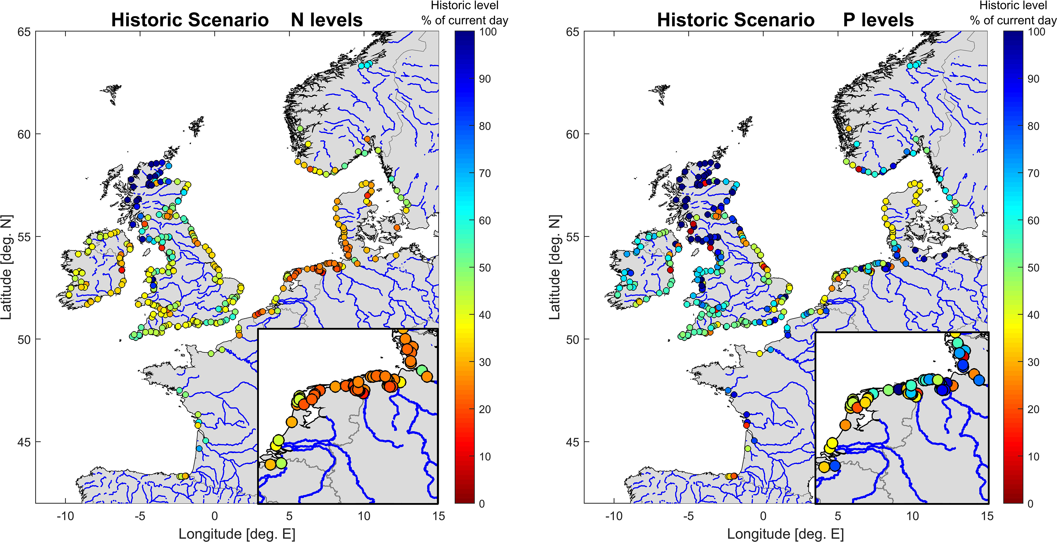
Figure 4 Pre-eutrophic riverine loads as percentages of current day loads. Left: pre-eutrophic N loads, right: pre-eutrophic P loads.

Estimates of atmospheric nitrogen deposition rates around 1900 were calculated based on the trends in TOxN and NH₃ emissions estimated by Schöpp et al. (2003) over Europe, including its marginal seas. These trends were then used to estimate the spatially resolved nitrogen deposition rate estimates by EMEP (2020) for the years 1890-1900 following the method of Große et al. (2016). Table 2 shows the current and pre-eutrophic atmospheric deposition rates estimated by Schöpp et al. (2003), and their ratio. These historic/current ratios are applied to current deposition fields from EMEP to estimate historic atmospheric deposition rates. Atmospheric phosphorous deposition rates were deemed negligible, both in the current state and historical scenario.

For the nutrient inputs across model open boundaries, we assumed that boundaries to the open sea were sufficiently far away from riverine sources to not be affected by nutrient reductions, and these were kept the same for CS and HS. For the Baltic boundary a different approach was taken, as the Baltic is highly eutrophic. As such, the pre-eutrophic boundary should reflect the historic nutrient status at the Darss sill and Drogden sill. Reduction percentages for nutrients at these locations were derived from a long model simulation (1850 – 2008) with the ERGOM model provided by Thomas Neumann (IOW, Germany). The resulting historic percentages (compared to current-day loads) are given in Table 3.

TABLE 3

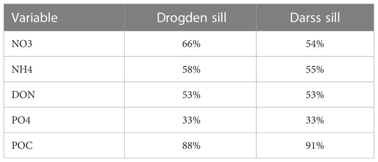
Table 3 Pre-eutrophic nutrient concentrations/loads? As percentage of current values for the Drogden and Darss sills in the Baltic Sea.

2.7 Weighted ensemble method

As models have varying skills in different areas, and variables, we applied the weighted ensemble approach of Almroth and Skogen (2010) to calculate ensemble averages. This method uses observations to determine a model’s skill in representing a certain variable in a certain area, and assigns appropriate weights to the model results. We applied these weights to calculate ensemble model averages for the OSPAR areas defined for the COMP4 assessment (section 2.4). Almroth and Skogen (2010) used this weighted ensemble approach to derive a better estimate of the current state, which was then assessed against the eutrophication criteria of the time. Here, we apply this method to obtain weights based on validation of current state results. We then applied these weights to the historic results and estimate the area’s pre-eutrophic state.

The applied weighting method is given by Eq. 1-Eq. 4 and is based on model results for the current state and the available observations from the COMPEAT tool. It relies on observational concentrations being available in each area over the chosen COMP3 period (2009-2014). As such, the weighting is applied to winter DIN and DIP and growing season mean Chl results. When observations were not available for a given area, we used the unweighted ensemble mean (i.e. a classical averaging was applied), but DIN, DIP and Chl weights were also applied to Total N, Total P and Chl P90, respectively. For Chl, the observations involved both in situ and satellite observations. In any given area, the cost function $C_i^P$(Eq. 1) was calculated for each model i and parameter P (e.g. DIN), with P ^obs and P ^{model ∈ CS} referring to the current state, observational and simulated values, respectively. Model results were averaged over the years 2009-2014 before application in the cost function: as such, a one-to-one comparison of individual stations is not included in the method. Individual model results for the cost function are shown in Appendix E, for the parameters DIN, DIP and Chl. Weights W were then calculated per model and per assessment area (Eq. 2) with B=0.1 an arbitrary constant to avoid division by small numbers in case of good model fits (Almroth and Skogen, 2010). The weights were then normalized using all contributing models in the area for each parameter (Eq. 3, with N the number of contributing models). Normalized weights from the current state were then applied to the model results obtained from the historic scenario (Eq. 4). Note that the number of contributing models varies with area and parameter, with a maximum of 7 (Southern Bight of the North Sea) and a minimum of 2 (Gulf of Biscay).

$\begin{array}{ll}{C}_i^P=\left|\frac{mean P_i^{model \in CS}-mean P^{obs}}{std P^{obs}}\right|& \text{Eq. 1}\end{array}$

$\begin{array}{ll}{W}_i^P=\frac{1}{C_i^P+B}& \text{Eq. 2}\end{array}$

$\begin{array}{ll}Wnor{m}_i^P=\frac{N}{{\sum }_{i=1}^N{W}_i^P}*W_i^P& \text{Eq. 3}\end{array}$

$\begin{array}{ll}WM{A}_{HS1}^P=\frac{1}{{\sum }_{i=1}^{N}Wnor{m}_i^P}*\sum _{i=1}^N(Wnor{m}_i^P*mean{P}_i^{model \in HS1})& \text{Eq. 4}\end{array}$

As the cost function is based only on the current state results, it inherently neglects differences in the individual model responses to the historic scenario, which is inevitable in absence of sufficient observations for the historic scenario. Weighted ensemble results are generally more robust than those of the individual members, as model strengths are enhanced and model weaknesses are reduced by the applied weighting.

3 Results

3.1 Annual results per model

First we show results for 2 areas in more detail: the Channel Well Mixed Tidally Influenced area (Figure 5) and the Southern North Sea area (Figure 6) (see Figure 3 for the locations of these assessment areas). Annual values per individual model are shown, as well as the number of available observations per year and their mean annual value. The overall observational mean, ensemble model mean and the weighted ensemble model mean over the original COMP4 assessment period (2006-2014) are also provided. Additional selected areas are shown in (Appendix H; Supplementary Figures 9-15). All data presented here are spatially averaged over the area and temporally averaged over the individual years.

FIGURE 5

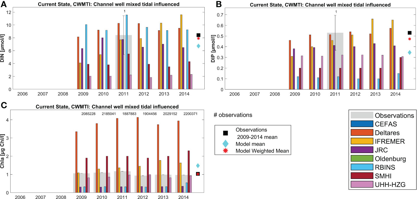
Figure 5 Annual results per model for area Channel Well Mixed Tidal Influenced (CWMTI, area 18): (A) DIN, (B) DIP and (C) Chl. The grey bars denote the observational values per year, including their standard deviation. Note the low number of observations for DIN and DIP.

FIGURE 6

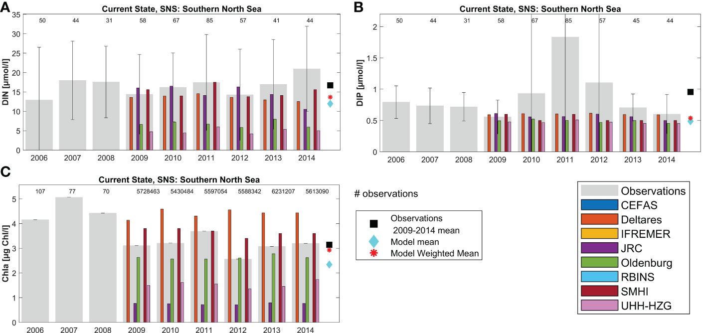
Figure 6 Annual results per model for area Southern North Sea (SNS, area 11): (A) DIN, (B) DIP and (C) Chl. The grey bars denote the observational values per year, including their standard deviation. The scale of subfigure B has been adjusted to show the individual results better: the DIP observational standard deviation for years 2010, 2011, 2012 was 1.38, 8.94 and 3.45 respectively.

Through the ensemble-weighted-mean method a more robust estimate can be made of nutrient and chlorophyll concentrations. Model estimates for specific variables in specific areas and years show large variability, with between-model variability generally larger than interannual variability within an area. The ensemble model mean (light-blue diamonds in Figures 5, 6) tends to be closer to the observed concentrations (black squares) than the individual model results. The weighted ensemble mean is even closer to the observed concentrations (red asterisks), but the ensemble model mean cannot get closer to the observations than the closest model result (e.g. Figure 6B, all models underestimate winter DIP concentrations in this area). The effectiveness of the weighted ensemble mean approach strongly depends on the availability and representativeness of observation data per assessment area. This is illustrated by Figure 5, where for both DIN and DIP only one observation was available in 6 years, leading to large uncertainty in the observational data that the weights are based upon. In contrast there are many more observed data available for chlorophyll in the same area, thanks to earth observation data. Note that in-situ observations for Chl tend to be higher than the mean EO Chl data.

In general, all models capture the yearly observational mean for DIN, DIP and Chl well for most areas. However, differences between models for each parameter exist. DIN results display high variability (overestimation as well as underestimation) but DIP is usually close to the observational range (Figures 5, 6; Supplementary Figures 9–15). Chl results show both large over- and underestimations. Note that the observational mean over 2009-2014 for an area may be biased towards the coast and fair-weather conditions. Limited numbers of observations per year can also introduce bias for individual areas, e.g. by missing concentration peaks.

3.2 Current state

The horizontal distribution of the weighted ensemble results for the present day for surface winter DIN, DIP and growing season Chl are displayed in Figure 7. High concentrations are found for all three variables in near-coastal and river plume areas, and in the Southern Bight of the North Sea. Highest concentrations for these indicators are found in the Scheldt plume (SCHPM1, SCHPM2), Meuse plume (MPM), Rhine plume (RHPM), and Seine plume (SPM), and to a lesser extent in the Elbe plume (ELPM). The weighted ensemble approach is thus capable of simulating known coastal gradients.

FIGURE 7

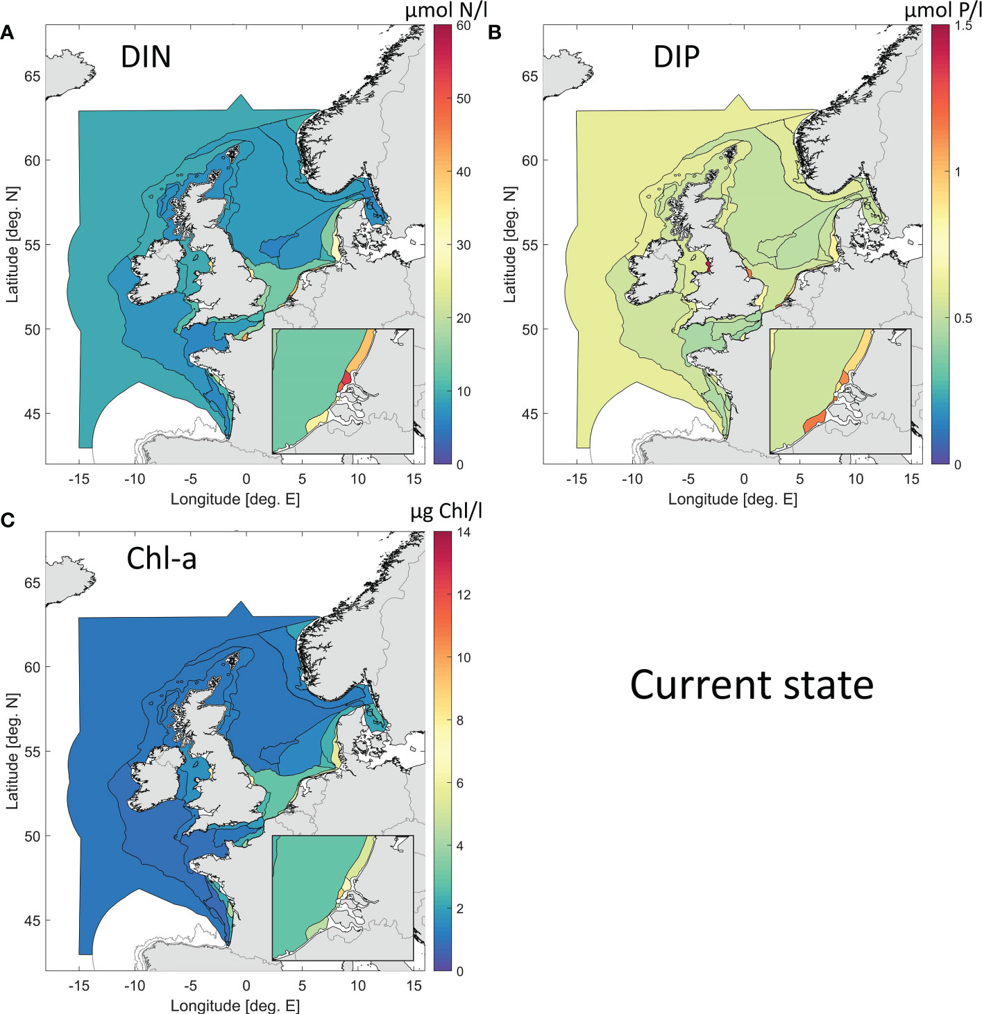
Figure 7 Weighted ensemble results for the current state (2009-2014 average), for surface DIN (A), DIP (B) and Chl (C).

3.3 Pre-eutrophic state

The horizontal distribution of the weighted ensemble results for the pre-eutrophic state (or HS) for surface winter DIN, DIP and growing season Chl are presented in Figure 8 and as a table in Appendix G (Supplementary Materials). Offshore results are similar to the current state results, but coastal areas (typically influenced by rivers) show consistent lower concentrations for all parameters.

FIGURE 8

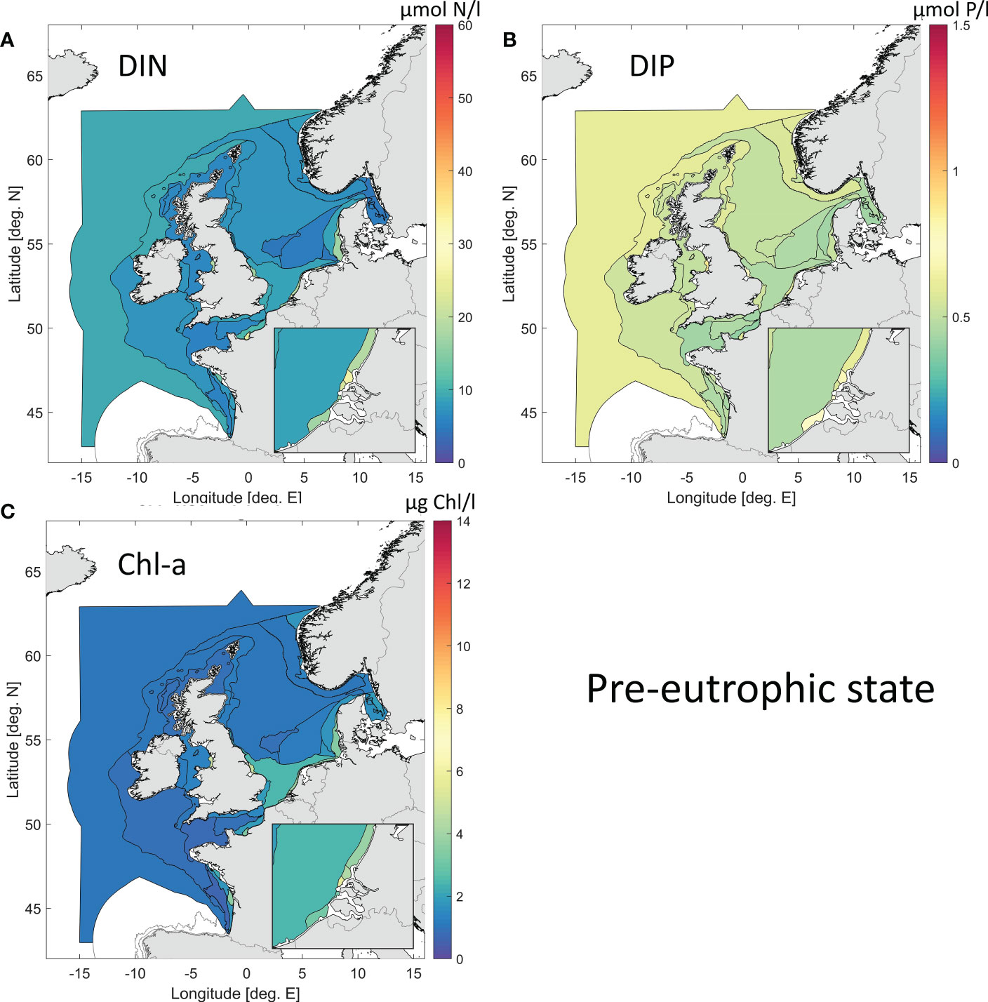
Figure 8 Weighted ensemble results for the pre-eutrophic state (~ 1900), for surface DIN (A), DIP (B) and Chl (C). The colour bar scale is identical to that of Figure 7.

3.4 Differences between current and pre-eutrophic state

The difference between the ensemble mean values for the pre-eutrophic state and the current state exhibits up to 50 - 60% less dissolved inorganic nutrients in the coastal zones in the pre-eutrophic state (Figure 9). Almost no changes are observed in oceanic areas, with at most a 1% difference. Note that in general a decrease in nutrient input can lead to local increases in some dissolved nutrients, as the input reduction of the limiting nutrient will decrease primary production, thus reducing nutrient uptake and causing a possible local increase in non-limiting nutrients. DIN levels were up to 62% lower in the pre-eutrophic state than in the current state, particularly along the Dutch and German coast. Both DIP and Chl concentrations were up to 40% lower in the pre-eutrophic state than in the current state. In contrast there is no effect of the DIP concentration within most of the Channel area and the coastal region of France while the difference for Chl lies around 20% in the Channel area and increases at the French coast. Also for the Eastern North Sea area, east of the Dogger Bank, the difference between the two simulations is higher for Chl than for DIP, but still lower than for DIN.

FIGURE 9

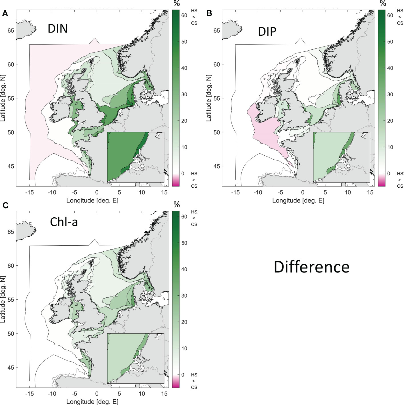
Figure 9 Difference between the weighted ensemble results for the current state (CS) and the pre-eutrophic state (historic scenario, HS) for DIN (A), DIP (B) and Chl (C). Green colours indicate areas where the pre-eutrophic levels were lower than those of the current state. Note that the colour bar extends to -5% only, indicating areas where pre-eutrophic levels were slightly higher than current levels.

Other eutrophication effects include N:P ratio changes, increased net primary production and low oxygen levels near the bed through remineralization of excess organic material by bacteria. Figure 10 shows the differences for the unweighted (due to lack of observations) ensemble mean differences for these eutrophication related phenomena. Both the N:P ratio and net primary production were much smaller for the pre-industrial state in the coastal zones (maxima of 35% and 30% respectively) than in the current state. Note that the net primary production reported here relates predominantly to pelagic production, as the models do not include macrophytes. Pre-eutrophic conditions are known for extensive macrophyte presence (Nienhuis, 1996), and would thus be characterized by a larger benthic primary production contribution. Near bed oxygen levels were higher in the Southern Bight of the North Sea, the English Channel area and the coastal parts of the Bay of Biscay under pre-eutrophic conditions. The Meuse plume is the only area where near bed O₂ levels were slightly lower (<1%) in the historic state. Oxygen values in the Bay of Biscay are dominated by 1 of only 2 contributing models: without weighting due to lack of observations outlier values can have disproportionate influence. The high value for O₂ difference in the Gironde Plume (GDPM, -50.7%) is deemed artificial, and this may also affect the adjacent water bodies (Gulf of Biscay Coastal Waters or GBCW: -22.1%).

FIGURE 10

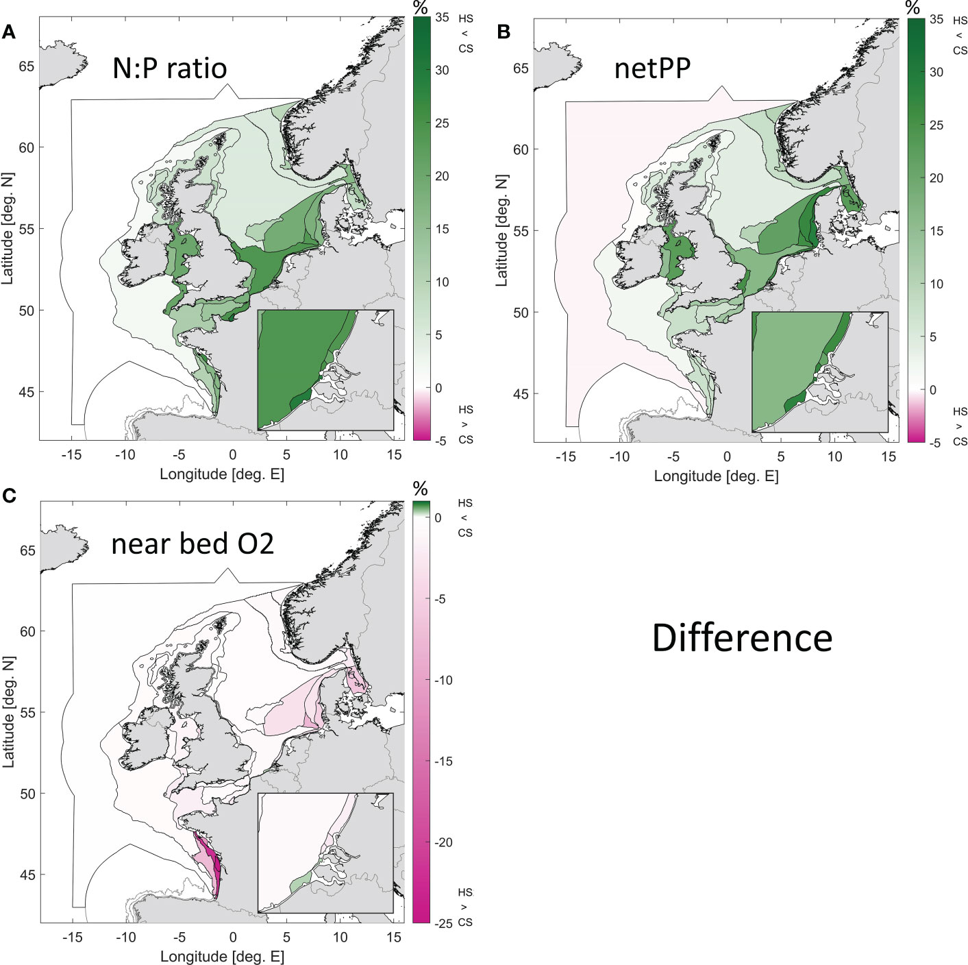
Figure 10 Difference between the ensemble results (unweighted) for the current state (CS) and the pre-eutrophic state (historic scenario, HS) for the N:P ratio (A), net primary production (B) and near bed oxygen levels (C). Green colours indicate areas where the pre-eutrophic levels were lower than those of the current state. Note the changing colour bar scale, for O₂ the scale starts at 1%.

3.5 Ecosystem sensitivity

The presented results clearly show the elevated nutrient concentrations in the coastal zone in the current state, compared to the pre-eutrophic state. The accompanying net primary production values as a function of winter total N and P concentrations are displayed in Figure 11 for all areas calculated by each model.

FIGURE 11

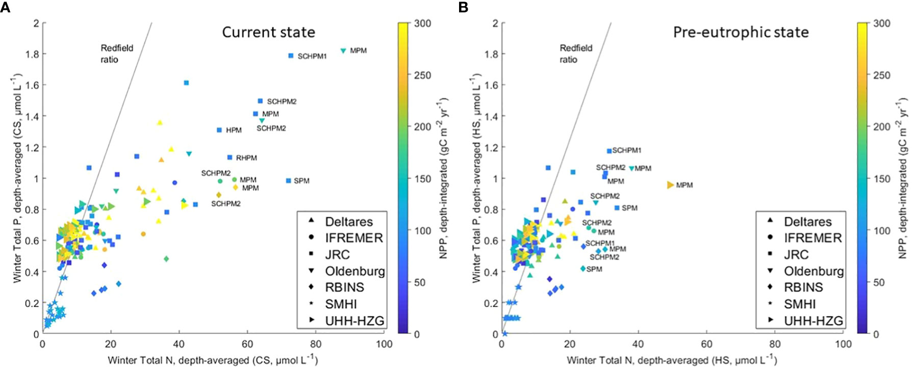
Figure 11 Model results of winter total phosphorus concentration (Ptot) as a function of winter total nitrogen concentration (Ntot) in each area for each model. (A) current conditions, (B) pre-eutrophic conditions (both 2009-2014). The colours indicate the modelled net primary production (NPP) for the corresponding areas and models. The line indicates the global ocean Redfield ratio (N:P = 16). Only some outlying results have been named, for area acronyms see Appendix C.

In the current state (Figure 11A) the relationship between modelled Total N and Total P tends to reproduce the Redfield ratio in offshore areas (characterized by low concentrations for both variables) but not in coastal areas where TN concentrations are high due to anthropogenic river loads. Areas showing N:P ratios far from Redfield are found close to the delta rivers outlets (Rhine, Meuse, Scheldt; areas RHPM, MPM, SCHPM1, SCHPM2), but also in the Humber plume (HPM) and the Seine plume (SPM) areas. This is a direct result of the successful phosphate loads reduction and less successful nitrogen loads reduction (Conley et al., 2009), showing higher impact in coastal than in offshore areas. N:P ratios for pre-eutrophic conditions (Figure 11B) are much lower in river plume areas than in the current state scenario. The N:P ratio varies between 55-25 molN molP-1 in the current state and between 30-15 molN molP-1 in the pre-eutrophic state in coastal areas (with exception of the Meuse Plume and Seine Plume, which remain on high N:P ratios). Note that the Redfield ratio is an average value applicable to global oceanic conditions, and that it is subject to high variability in the short term especially in coastal waters (Falkowski, 2000). There are exceptions where the dual reduction does not significantly change the N:P ratio, which remains as high as 42 molN molP^-1 or even 50 molN molP^-1 for e.g. the Meuse Plume area. Despite differences between models (results not shown), net primary production (NPP) decreases in the pre-eutrophic scenario compared to present conditions (Figure 10B).

Since all models apply the same river loads, the differences in TN and TP concentrations between models in coastal areas are due to other differences in the models’ ecological and hydrodynamic set-up, such as the model grid resolution and domain and ecological process formulations. The proximity of boundary conditions may influence concentrations in an area, for some of the smaller domain models this can be near river plume areas. To focus on the impact of different formulations of ecological processes and exclude the influence of the underlying hydrodynamic model we compared relative changes in chlorophyll mean concentrations with relative changes in nutrient concentrations (Figure 12). Some models, such as the Deltares and RBINS models show decreases in Chl concentrations almost proportional to decreases in DIN concentrations (close to the black line). Other models such as the JRC model and Oldenburg model show a much smaller response in Chl concentrations to decreasing winter nutrient concentrations.

FIGURE 12

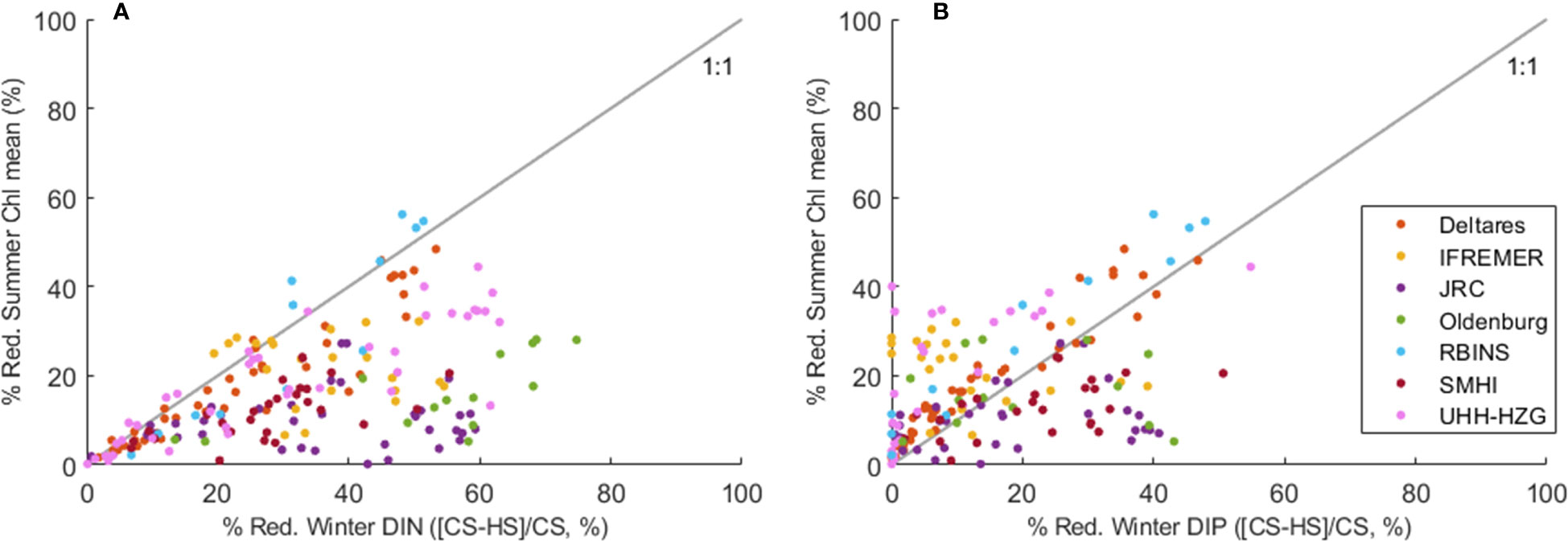
Figure 12 Relative reduction of growing-season mean Chl as a function of the relative reduction of winter DIN (A) and winter DIP (B). Each dot indicates a marine area for one model and models are differentiated by colours.

Here we see how a relative reduction in winter nutrient concentrations (pre-eutrophic state compared to current state, [CS-HS]/CS) induces a relative reduction in mean Chl. The relative reductions in winter DIN were in general stronger (up to ~75%) than the reductions in winter DIP (up to ~55%) in the individual model results. Due to the already achieved P reduction measures between peak discharges in the 1980’s and the current state period, we observe smaller differences for winter DIP between pre-eutrophic and current loads in our model study. The corresponding reductions in mean Chl reach 60% at most. In many areas, the required reductions in nutrients to reach the pre-eutrophic mean Chl seem higher for DIN than for DIP. Although the relationship between winter nutrients and mean Chl is non-linear and perturbed by other factors like the underwater light climate, grazing and regeneration of nutrients, the results suggest that certain areas are less sensitive to further DIN reduction than others. These are mainly coastal areas where DIP is likely the limiting nutrient already, due to the successful reductions in riverine P loads (Billen et al., 2011).

4 Discussion

4.1 Eutrophication on the European shelf

We have presented our ensemble results for the pre-eutrophic state of marine waters on the European Shelf. This estimate of pre-eutrophic conditions follows the steps taken by OSPAR to move towards a harmonized and integrated eutrophication assessment across the North-East Atlantic, taking into account the Water Framework Directive (WFD; EC, 2000) and Marine Strategy Framework Directive (MSFD; EC, 2008), which require the definition of a common ‘baseline’ to which the eutrophication status of waters can be compared. The approach, to define ecologically relevant threshold levels for eutrophication indicators (built on an agreed baseline and acceptable deviation thereof), includes the definition of a so-called “reference status” related to marine conditions undisturbed by anthropogenic inputs. As there are no suitable areas undisturbed by anthropogenic pressures that can serve as a reference area for the North-East Atlantic, an alternative method is to define a “historic” reference that represents a pre-eutrophic state (EC, 2003). Since observations from such a period are lacking, these conditions will have to be estimated using ecosystem models. The objective of this study is therefore to define a common baseline representing pre-eutrophic conditions. This is a significant step forward towards science-based and coherent thresholds for marine eutrophication management, and away from previous thresholds based on expert judgment and national modelling efforts, and applied to nationally set assessment areas.

The pre-eutrophic conditions shown in this study are not identical to pristine conditions (i.e. complete removal of anthropogenic influences and Europe largely covered in woods, see Billen & Garnier (1997)). In a previous study, Desmit et al. (2018) reported that the N:P ratio averaged across the coastal North-East Atlantic would be lowered from ~35 molN molP^-1 under current conditions to ~11 molN molP^-1 under pristine conditions, which would foster diatoms and reduce the impact of Phaeocystis globosa in the southern bight of the North Sea. Here, the N:P ratio shows a decrease of similar magnitude, with a N:P ratio of 55-25 molN molP^-1 in the current state and of 30-15 molN molP^-1 in the pre-eutrophic state, suggesting that pre-eutrophic conditions may be sufficient to induce desirable phytoplankton community structures. Although most coastal systems of the North Sea are P-limited in the spring rather than N-limited, the high N:P ratios in many coastal areas would argue against further P reduction measures without accompanying N reductions as the N:P ratio shapes the structure of the phytoplankton communities (Cloern, 2001; Conley et al., 2009). Therefore, any shift in this ratio should be applied to improve the phytoplankton community structure, and not foster undesirable species (Radach and Moll, 1990; Prins et al., 2012).

4.2 Importance of observational data

Observational data are of prime importance for the applied approach: as input data, as validation data and as data used for weighting different model results in the ensemble. This immediately highlights issues with both availability of observations and their temporal and spatial resolution.

Chlorophyll a levels encompass diatom contributions, but these phytoplankton can only grow when silicate is available for them to build their cell walls. In the applied riverine inputs database information on silicate is lacking for Belgian, Danish, Irish and Spanish rivers. Total nitrogen data is lacking for British and Spanish rivers. Without realistic values for these nutrient inputs the models will invariably struggle to reproduce observed concentrations in the adjacent coastal zones. More coordinated riverine monitoring within Europe and subsequent central storage of sample data for easy access could address these issues.

The observations used in the weighting method were obtained from the COMPEAT tool built by OSPAR, that draws on the ICES marine database (Supplementary Materials Figure S1). Even though N and P are the main driving nutrients of primary production in shelf seas and therefore constitute the basis of our understanding of eutrophication processes, measurements of N and P concentrations in many areas (for example the Channel Well Mixed Tidally Influenced; CWMTI, Figure 5) are severely limited in number. This complicates comparison with model results offering more temporal and spatial resolution, and increases uncertainty. Figure S1 in the supplementary materials highlights the spatial bias of the observations (available mainly in near-coastal zones), while the annual results (Figures S9-S15, Appendix F) highlight issues with temporal observational coverage. It is therefore not surprising that cost function results for the individual models (Appendix E) regularly show moderate or poor results. To have a good fit, the model results, averaged over all simulated years and the entire assessment area, should compare well with limited observations, mainly taken in the coastal zone during daylight hours in fair weather conditions. This discrepancy does not diminish the validity of observations, rather it highlights both their importance and their limitations (Skogen et al., 2021). In order to improve the applied method more observations in time and space are needed. Thereby, models can indicate where measurements are most needed to improve spatial and temporal coverage with respect to the processes being measured (Ferrarin et al., 2021).

Within this exercise the added value of the satellite data for Chl has been clear, ensuring weighting factors for Chl in all assessment areas. The integration of in-situ and EO Chl data is an optimal remote sensing approach to provide water surface properties in coastal regions with high temporal and spatial resolution (Arabi et al., 2020). As such, Chl in-situ measurements are also vital, and more are needed. Note that satellites observe wavelength, and that a mathematical model is applied to derive surface chlorophyll a data from these. By including observations in the weighted results, the related observational uncertainties (due to limited data availability) are also imported. Improved observational coverage could mitigate this.

4.3 Level of confidence in model outputs

All models used in this exercise have been extensively validated, and their respective cost functions are shown in Appendix E. Some models generally underestimate mean concentrations while others overestimate them: the ensemble approach ensures a balanced response. For chlorophyll a it is apparent that two models overestimate Chl concentrations (Deltares, SMHI) while the others show a consistent underestimation. In river plume areas Chl tends to be underestimated by nearly every model (Appendix F). The scatter plot of modelled weighted-average Chl P90 versus winter DIN in each area displays a linear relationship (results not shown, r² > 0.81). The slope of this relationship is 0.34 µg Chl/µmol N, which is significantly lower than the slopes obtained from long time series on the Belgian and Dutch continental shelves, displaying respective values of 0.6 and 1.2 µg Chl/µmol N (Desmit et al., 2015). Although the models deliver fairly good results for nutrient concentrations, the modelled Chl concentrations are often lower than expected, and this must be considered carefully in any further application. In all applied models the Chl concentration is mainly determined by nutrient availability, light availability and grazing pressure. Differences can thus stem from the complexity of included nutrient recycling processes, hydrodynamic differences in nutrient and suspended particulate matter transport, inclusion of benthic storage and release of nutrients, inclusion of a separate sediment resuspension model and the complexity of zooplankton representation. For example, the Deltares model does not include zooplankton, while the SMHI model has the lowest number of pelagic state variables, indicating lower pelagic complexity (Appendix E). Whether these model characteristics contribute to the observed high Chl concentrations from these models needs further careful analysis though. The same applies to those models that have consistently low Chl predictions compared to observations. Lack of phytoplankton species resolution in the models (usually 2-6 different functional groups) can also play a part in underestimating Chl levels (unlikely to capture a single species sudden bloom event well), as can the applied Chl:C ratio used to calculate the Chl concentrations in models based on the simulated phytoplankton biomass. Reappraisal of individual model results and possible model improvement is thus a key part of ensemble modelling.

Structural diversity of the models, parametric uncertainties, differences in spatial resolution, in boundary conditions and in forcings will necessarily cause differences between model estimates. Although some of these issues have been solved in this exercise by applying identical loads, forcings and boundary conditions, there is still variability in model responses. This variability is desirable as it displays a range of possible outcomes, and ensemble modelling approaches are used to explore and quantify this diversity. Though parametric variation for each ensemble member would enhance confidence in the individual results even further, a separate parametric ensemble for each contribution to the overall ensemble is generally unfeasible due to computational and financial restraints. Note that we applied the weighting method by Almroth and Skogen (2010) in a fundamentally different way from the original article: they used it to enhance the quality of the modelled current state in order to compare it against thresholds whereas in this study we applied it to a pre-eutrophic scenario which can be used to derive thresholds.

An objective way to further reduce uncertainties is to resort to weight-averaged values, estimated from the comparison between model outputs and observations, and apply these weights to the individual model results before taking the ensemble average (Almroth and Skogen, 2010). The present exercise used this weighted-ensemble-mean method to provide pre-eutrophic values, or reference values, for the indicators of eutrophication in coastal and shelf areas. For this the availability of observational data in the COMPEAT tool was essential. More observational evidence would therefore also increase confidence in the weighted ensemble result.

4.4 Ensemble modelling as a tool for marine management

In the past several single model approaches have been used to estimate the pre-eutrophic state of marine systems (Schernewski and Neumann, 2005; Schernewski et al., 2015; Kerimoglu et al., 2018), including using multiple single models to cover a larger area (Desmit et al., 2018). Ensemble modelling addresses the inherent uncertainties in single model results and is increasingly applied in marine response studies (Almroth and Skogen, 2010; Lenhart et al., 2010; Eilola et al., 2011; Meier et al., 2019; Friedland et al., 2021; Stegert et al., 2021) despite the higher efforts involved. These efforts include the necessity to combine a variety of modelling groups and their individual models, as well as agreement to a common protocol to ensure comparable results, agreement on suitable scenarios and to a common analysis of the obtained scenario results. Individual funding issues can undermine this common approach, as can technical issues as demonstrated here (lack of results from one participating model). Both pecuniary and technical issues can result in gaps in geopolitical coverage of the ensemble result that can hinder international acceptance of derived policy products. However, the benefits of ensemble modelling are equally clear: increased confidence in the results (due to the inclusion of different models with their own specific strengths), more insight into model dynamics and the opportunity for individual model development (based on the ensemble results and individual performance) and a higher level of acceptance on the international (policy) stage compared to single model results.

Thus, ensemble modelling is a suitable approach to help tackle a variety of ecological issues and their management in the marine environment. This could include dispersal of harmful dissolved substances, marine litter dispersion (by using particle tracking models), circulation pathways of pathogens (by using epidemiological bio-physical models) and impacts of these and other stressors on ecosystem services (coupled ecosystem models). Models are extremely suited to test different policy options, quantify single and combined stressor impacts and predict future marine environmental conditions and their impact on anthropogenic derived usage. They can do this on both small (harbours, estuaries, bays) and large (basins, oceans) scales, providing a broad answer to marine ecosystem response that augments observational evidence and dedicated experimental work. It is therefore anticipated that ensemble modelling will be increasingly used in marine management issues.

5 Conclusions

This study presented a weighted ensemble modelling approach to estimate the pre-eutrophic state of the marine ecosystem on the European Shelf. Eight modelling centers from countries around Europe participated with their most suited ecosystem model, though only seven delivered results on time. Inputs and boundary conditions were aligned as much as possible to focus on the models’ response to pre-industrial riverine and atmospheric nutrient levels. As expected, results showed lower nutrient concentrations in the pre-eutrophic state in most coastal areas, whereas offshore areas showed minimal change compared to the current state. DIN, DIP and Chl levels were at most 62%, ~40% and ~40% lower in the pre-eutrophic state than they are now, respectively, with most changes occurring in the southern North Sea, the Irish Sea and coastal Bay of Biscay areas. Net primary production was also lower in the historic scenario, with reductions up to ~35% concentrated in the South-eastern North Sea and the Irish Sea. N:P ratio showed little change in offshore areas, but strong changes in coastal areas, which moved closer to the Redfield ratio in the historic scenario. Pre-eutrophic results for near-bed oxygen levels showed improvements in known problem areas such as the Oyster Grounds. Overall, coastal areas show more sensitivity to DIP reductions than DIN reductions.

The resulting concentration estimates for key eutrophication indicators like surface winter DIN, DIP and growing-season chlorophyll-a can be used as a basis for assessments as well as policy measures to combat marine eutrophication. It also illustrates the potential of modelling to support marine management. However, the weighted ensemble method relies on observations, and more and more spatio-temporally balanced observations are needed, particularly in offshore areas, to augment the applied weighting method and reduce uncertainty even further. As such, this work highlights the need for (more) extensive monitoring programmes. Models can help in this respect by optimizing existing and new observational efforts. While models are able to focus on local ecosystem functioning, they also consider the continuity of transboundary transport and processes across large areas. This model specificity is particularly useful in systems where data collection remains a challenge, such as the ocean. In that sense, models will continue to be useful for policy initiatives in coastal management, and uptake by marine managers is encouraged.

The ensemble approach presented here has demonstrated its use for policy purposes by defining a baseline for nutrient reduction measures; it may be useful for other environmental questions as well. For eutrophication modelling the next step should be to consider climate change impacts on the marine environment, and how these changes impact on derived thresholds for eutrophication indicators, both in the immediate and intermediate (policy) future.

Data availability statement

The datasets presented in this study can be found in online repositories. The riverine input data used for all scenarios can be found here: https://doi.org/10.25850/nioz/7b.b.vc. The other open sources are mentioned in the manuscript.

Author contributions

Model simulations were performed by AB, LV, AvdL, CS, XD, GL, OK, IB, TS, RF and MP. All authors contributed to the ensemble methodology and conditions, which was led by H-JL. TP led the discussions with associated groups within OSPAR, while LF performed most of the work related to COMPEAT. SL provided the riverine data, collected the individual results and produced the final tables and most of figures, with additional analysis figures provided by XD and RF. All authors contributed to the article and approved the submitted version.

Funding

We would like to thank the Swedish Agency for Marine and Water Management for their support and financial contribution to this work. CS and RF were supported by the Umweltbundesamt (UBA, grant no. 3718252110 and 3720252020). Supercomputing power was provided to RF by HLRN (North-German Supercomputing Alliance) and to CS by Deutsches Klima-Rechenzentrum (DKRZ). OK was supported by the Deutsche Forschungsgemeinschaft (DFG, KE1970/2-1). MP acknowledges the Pôle de Calcul et de Données Marines (PCDM) for providing supercalculator DATARMOR {storage, data access, computational resources}. SL was supported by Rijkswaterstaat and NIOZ. Deltares was supported by Rijkswaterstaat and the European Maritime and Fisheries Fund. Deltares and IFREMER were partly supported by the Jerico-S3 project, funded by the European Union’s Horizon 2020 research and innovation programme under grant agreement No 871153. RBINS received financial support from BELSPO through the project ReCAP, which is part of the Belgian research program FED-tWIN.

Acknowledgments

We like to thank Thomas Neumann (IOW) and Stiig Markager (Aarhus University) for their contribution to derive pre-eutrophic boundary condition for the Baltic Sea outflow. A very special thanks to Hjalte Parmer for providing the ICES data that are used within the COMPEAT tool. We thank the members of ICG-Eut and TG-COMP for the fruitful discussions, as well as OSPAR for commissioning this work. Part of the maps in this manuscript were made using the free package M_Map: Pawlowicz, R., 2020. “M_Map: A mapping package for MATLAB”, version 1.4m, [Computer software], available online at www.eoas.ubc.ca/~rich/map.html. Computing facilities for Deltares were provided by the DECI resource Cartesius based in The Netherlands at SURFsara with support from PRACE. The support of Maxime Mogé from SURFsara, The Netherlands is gratefully acknowledged. UK riverine data was processed from raw data provided by the Environment Agency, the Scottish Environment Protection Agency, the Rivers Agency (Northern Ireland) and the National River Flow Archive. French water quality data was provided by Agence de l’eau Loire-Bretagne, Agence de l’eau Seine-Normandie and IFREMER, while flow data was provided by Banque Hydro. German and Dutch riverine data was provided by the University of Hamburg (Johannes Paetsch, Hermann Lenhart), with some additional German river data supplied by IOW (Ulf Graewe). Irish flow data was provided by Hydrodata and the Environment Protection Agency (Hydronet), while water quality data was obtained from OSPAR RID reports. Norwegian flow data was supplied by NVE’s Anne Fleig (afl@nve.no), water quality data was obtained from NIVA (www.niva.no) and Tore Høgåsen (tore.hogaasen@niva.no). Danish water quality data was provided by the National Environmental Research Institute (NERI). Water quality data for Baltic rivers was provided by the University of Stockholm and the Baltic Nest (www.balticnest.org/bed). Spanish data was provided by Dr. Luz Garcia (while at Cefas, UK). Portuguese data was obtained from Dr. Amelia Araujo (Cefas, UK). Dr. S. M. van Leeuwen, NIOZ, Lansdiep 4, ‘t Horntje, Texel, the Netherlands, pers. comm.

Conflict of interest

The authors declare that the research was conducted in the absence of any commercial or financial relationships that could be construed as a potential conflict of interest.

The reviewer JB declared a shared affiliation Helmholtz Centre for Materials and Coastal Research with the author CS to the handling editor.

Publisher’s note

All claims expressed in this article are solely those of the authors and do not necessarily represent those of their affiliated organizations, or those of the publisher, the editors and the reviewers. Any product that may be evaluated in this article, or claim that may be made by its manufacturer, is not guaranteed or endorsed by the publisher.

Supplementary material

The Supplementary Material for this article can be found online at: https://www.frontiersin.org/articles/10.3389/fmars.2023.1129951/full#supplementary-material

References

Almroth E., Skogen M. D. (2010). A north Sea and Baltic Sea model ensemble eutrophication assessment. Ambio 39 (1), 59–69. doi: 10.1007/s13280-009-0006-7

PubMed Abstract | CrossRef Full Text | Google Scholar

Arabi B., Salama M. S., Pitarch J., Verhoef W. (2020). Integration of in-situ and multi-sensor satellite observations for long-term water quality monitoring in coastal areas. Remote Sens. Environ. 239, 111632. doi: 10.1016/j.rse.2020.111632

CrossRef Full Text | Google Scholar

Berdalet E., Fleming L. E., Gowen R., Davidson K., Hess P., Backer L. C., et al. (2016). Marine harmful algal blooms, human health and wellbeing: challenges and opportunities in the 21st century. Mar. Biol. Assoc. 96 (1), 61–91.

Google Scholar

Billen G., Garnier J. (1997). The phison river plume: coastal eutrophication in response to changes in land use and water management in the watershed. Aquat. microbial Ecol. (Cambridge, UK: Cambridge University Press) 13 (1), 3–17. doi: 10.3354/ame013003

CrossRef Full Text | Google Scholar

Billen G., Garnier J., Deligne C., Billen C. (1999). Estimates of early-industrial inputs of nutrients to river systems: implication for coastal eutrophication. Sci. Total Environ. 243, 43–52.

PubMed Abstract | Google Scholar

Billen G., Silvestre M., Grizzetti B., Leip A., Garnier J., Voss M., et al. (2011). “Nitrogen flows from European watersheds to coastal marine waters,” in The European nitrogen assessment: sources, effects, and policy perspectives. Ed. Sutton M. A. (Cambridge, UK: Cambridge University Press), 271–297. Available at: https://centaur.reading.ac.uk/28381/1/Chapter%2013%20ENA%20Billen%20et%20al%202011.pdf.

Google Scholar

Brockmann U., Topcu D. H. (2002). Nutrient atlas of the central and northern North Sea.

Google Scholar

Burkholder J. M., Tomasko D. A., Touchette B. W. (2007). Seagrasses and eutrophication. J. Exp. Mar. Biol. Ecol. 350 (1-2), 46–72.

Google Scholar

Ciavatta S., Brewin R. J. W., Skakala J., Polimene L., de Mora L., Artioli Y., et al. (2018). Assimilation of ocean-color plankton functional types to improve marine ecosystem simulations. J. Geophys. Res. C Oceans 123 (2), 834–854. doi: 10.1002/2017JC013490

CrossRef Full Text | Google Scholar

Claussen U., Zevenboom W., Brockmann U., Topcu D., Bot P. (2009). “Assessment of the eutrophication status of transitional, coastal and marine waters within OSPAR,” in Eutrophication in coastal ecosystems (Dordrecht: Springer), 49–58.

Google Scholar

Cloern J. E. (2001). Our evolving conceptual model of the coastal eutrophication problem. Mar. Ecol. Prog. Ser. 210, 223–253. doi: 10.3354/meps210223

CrossRef Full Text | Google Scholar

Conley D. J., Paerl H. W., Howarth R. W., Boesch D. F., Seitzinger S. P., Havens K. E., et al. (2009). Controlling eutrophication: nitrogen and phosphorus. Science 323 (5917), 1014–1015. Available at: https://citeseerx.ist.psu.edu/document?repid=rep1&type=pdf&doi=89c56da0503c6d284fee938932e1c20112e6197e.

PubMed Abstract | Google Scholar

Desmit X., Lacroix G., Thieu V., Menesguen A., Dulière V., Campuzano F., et al. (2015) EMOSEM final report-ecosystem models as support to eutrophication management in the north Atlantic ocean. Available at: https://archimer.ifremer.fr/doc/00292/40301/.

Google Scholar

Desmit X., Thieu V., Billen G., Campuzano F., Dulière V., Garnier J., et al. (2018). Reducing marine eutrophication may require a paradigmatic change. Sci. Total Environ. 635, 1444–1466. doi: 10.1016/j.scitotenv.2018.04.181

PubMed Abstract | CrossRef Full Text | Google Scholar

Diaz R. J., Rosenberg R. (2008). Spreading dead zones and consequences for marine ecosystems. Science 321 (5891), 926–929.

PubMed Abstract | Google Scholar

Donnelly C., Arheimer B., Capell R., Dahné J., Strömqvist J. (2013). Regional overview of nutrient load in Europe–challenges when using a large-scale model approach, e-HYPE. Proceedings of H04, IAHS-IAPSO-IASPEI Assembly, Gothenburg, Sweden, July 2013 (IAHS Publ. 361, 2013). Available at: https://iahs.info/uploads/dms/15569.10-49-58-361-06-H04_Donnelly_reviewed_CD20130403CORR.pdf.

Google Scholar

Duarte C. M., Conley D. J., Carstensen J., Sánchez-Camacho M. (2008). Return to neverland: Shifting baselines affect eutrophication restoration targets. Estuar. Coasts 32, 29–36. doi: 10.1007/s12237-008-9111-2

CrossRef Full Text | Google Scholar

EC (2000). Water framework directive (Directive 2000/60/EC) of the European parliament and of the council of 23 October 2000 establishing a framework for community action in the field of water policy. Eur. Commission Brussels. L327, 72 pp. Available at: https://eur-lex.europa.eu/legal-content/en/ALL/?uri=CELEX%3A32000L0060.

Google Scholar

EC (2003). “Guidance document no 5. transitional and coastal waters – typology, reference conditions and classification systems,” in Common implementation strategy for the water framework directive (Luxemburg: European Commission), 107. Available at: https://op.europa.eu/en/publication-detail/-/publication/eb740a3e-2df9-45c8-bf56-2ba75088f64f/language-en/format-PDF/source-276054079.

Google Scholar

EC (2008). Marine strategy framework directive (Directive 2008/56/EC) of the European parliament and of the council directive establishing a framework for community action in the field of marine environmental policy. Eur. Commission Brussels. L164, p. 19–40. Available at: https://eur-lex.europa.eu/legal-content/EN/TXT/?uri=celex%3A32008L0056.

Google Scholar

Edman M., Omstedt A. (2013). Modeling the dissolved CO₂ system in the redox environment of the Baltic Sea. Limnol. Oceanogr. 58 (1), 74–92. doi: 10.4319/lo.2013.58.1.0074

CrossRef Full Text | Google Scholar

Eilola K., Gustafsson B. G., Kuznetsov I., Meier H. E. M., Neumann T., Savchuk O. P. (2011). Evaluation of biogeochemical cycles in an ensemble of three state-of-the-art numerical models of the Baltic Sea. Mar. Syst. 88 (2), 267–284. doi: 10.1016/j.jmarsys.2011.05.004

CrossRef Full Text | Google Scholar

EMEP (2020). Transboundary particulate matter, photo-oxidants, acidifying and eutrophying components (Oslo, Norway: MSC-W & CCC & CEIP, Norwegian Meteorological Institute (EMEP/MSC-W). Available at: https://www.diva-portal.org/smash/get/diva2:1527049/FULLTEXT01.pdf.

Google Scholar

Enserink L., Blauw A., van der Zande D., Markager S. (2019). Summary report of the EU project ‘Joint monitoring programme of the eutrophication of the north Sea with satellite data’ (Ref: DG ENV/MSFD second Cycle/2016) (Belgium: REMSEM), 21.

Google Scholar

Falkowski P. G. (2000). Rationalizing elemental ratios in unicellular algae. J. Phycology 36 (1), 3–6. doi: 10.1046/j.1529-8817.2000.99161.x

CrossRef Full Text | Google Scholar

Ferrarin C., Bajo M., Umgiesser G. (2021). Model-driven optimization of coastal sea observatories through data assimilation in a finite element hydrodynamic model (SHYFEM v. 7_5_65). Geoscientific Model. Dev. 14 (1), 645–659. doi: 10.5194/gmd-14-645-2021

CrossRef Full Text | Google Scholar

Frederiksen M., Krause-Jensen D., Holmer M., Laursen J. S. (2004). Long-term changes in area distribution of eelgrass (Zostera marina) in Danish coastal waters. Aquat. Botany. 78 (2), 167–181. doi: 10.1016/j.aquabot.2003.10.002

CrossRef Full Text | Google Scholar

Friedland R., Macias D., Coassarini G., Daewel U., Estournel C., Garcia-Gorriz E., et al. (2021). Effects of nutrient management scenarios on the marine eutrophication indicators: a pan-European, multi-model assessment in support of the marine strategy framework directive. Front. Mar. Sci. 8. doi: 10.3389/fmars.2021.596126

CrossRef Full Text | Google Scholar

Gadegast M., Venohr M. (2015). Modellierung historischer nährstoffeinträge und-frachten zur ableitung von nährstoffreferenz-und orientierungswerten für mitteleuropäische flussgebiete. Bericht erstellt im Auftrag Des. NLWKN 39, 1875–1944.

Google Scholar

Garcia-Garcia L. M., Sivyer D., Devlin M., Painting S., Collingridge K., van der Molen J. (2019). Optimizing monitoring programs: A case study based on the OSPAR eutrophication assessment for UK waters. Front. Mar. Sci. 5. doi: 10.3389/fmars.2018.00503

CrossRef Full Text | Google Scholar

Greenwood N., Parker E. R., Fernand L., Sivyer D. B., Weston K., Painting S. J., et al. (2010). Detection of low bottom water oxygen concentrations in the north sea; implications for monitoring and assessment of ecosystem health. Biogeosciences 7 (4), 1357–1373. doi: 10.5194/bg-7-1357-2010

CrossRef Full Text | Google Scholar

Große F., Greenwood N., Kreus M., Lenhart H.-J., Machoczek D., Pätsch J., et al. (2016). Looking beyond stratification: A model-based analysis of the biological drivers of oxygen deficiency in the north Sea. Biogeosciences 13, 2511–2535. doi: 10.5194/bg-13-2511-2016

CrossRef Full Text | Google Scholar

ICES (2022). ICES data portal (Copenhagen: ICES). Available at: https://data.ices.dk/view-map. Dataset on Ocean HydroChemistry.

Google Scholar

ICG-EMO (2021). European Daily riverine flow and nutrient database. doi: 10.25850/nioz/7b.b.vc

CrossRef Full Text | Google Scholar

Jickells T. D. (1998). Nutrient biogeochemistry of the coastal zone. Science 281 (5374), 217–222.

PubMed Abstract | Google Scholar

Kerimoglu O., Große F., Kreus M., Lenhart H. J., van Beusekom J. E. (2018). A model-based projection of historical state of a coastal ecosystem: Relevance of phytoplankton stoichiometry. Sci. Total Environ. 639, 1311–1323. doi: 10.1016/j.scitotenv.2018.05.215

PubMed Abstract | CrossRef Full Text | Google Scholar

Kissel D. E. (2014). The historical development and significance of the haber Bosch process. Better Crops Plant Food 98 (2), 31.

Google Scholar

Krause-Jensen D., Duarte C. M., Sand-Jensen K., Carstensen J. (2021). Century-long records reveal shifting challenges to seagrass recovery. Glob. Change Biol. 27 (3), 563–575. doi: 10.1111/gcb.15440

CrossRef Full Text | Google Scholar

Lavigne H., van der Zande D., Ruddick K., Dos Santos J. C., Gohin F., Brotas V., et al. (2021). Quality-control tests for OC4, OC5 and NIR-red satellite chlorophyll-a algorithms applied to coastal waters. Remote Sens. Environ. 255, 112237. doi: 10.1016/j.rse.2020.112237

CrossRef Full Text | Google Scholar

Lenhart H.-J., Mills D. K., Baretta-Bekker H., van Leeuwen S. M., van der Molen J., Baretta J. W., et al. (2010). Predicting the consequences of nutrient reduction on the eutrophication status of the north Sea. J. Mar. Syst. 81, 148–170. doi: 10.1016/j.jmarsys.2009.12.014

CrossRef Full Text | Google Scholar

Mantikci A. M. (2014). Significance of plankton respiration for productivity in coastal ecosystems (Doctoral dissertation, PhD dissertation (Aarhus: Aarhus University).

Google Scholar

McCrackin M. L., Jones H. P., Jones P. C., Moreno-Mateos D. (2017). Recovery of lakes and coastal marine ecosystems from eutrophication: A global meta-analysis. Limnol. Oceanogr. 62 (2), 507–518. doi: 10.1002/lno.10441

CrossRef Full Text | Google Scholar

Meier H. M., Edman M., Eilola K., Placke M., Neumann T., Andersson H. C., et al. (2019). Assessment of uncertainties in scenario simulations of biogeochemical cycles in the Baltic Sea. Front. Mar. Sci. 6, 46. doi: 10.3389/fmars.2019.00046

CrossRef Full Text | Google Scholar

Nienhuis P. H. (1996). “The north sea coasts of Denmark, Germany and the Netherlands,” in Marine benthic vegetation: recent changes and the effects of eutrophication. Schramm/Nienhuis (eds) (Springer-Verlag Berlin Heidelberg:Marine Benthic Vegetation) 123, 187–221. Available at: https://www.researchgate.net/profile/Piet-Nienhuis/publication/254815397_The_North_Sea_Coasts_of_Denmark_Germany_and_The_Netherlands/links/56865ede08ae1e63f1f5769f/The-North-Sea-Coasts-of-Denmark-Germany-and-The-Netherlands.pdf.

Google Scholar

Nixon S. W. (2009). “Eutrophication and the macroscope,” in Eutrophication in coastal ecosystems (Netherlands: Springer), 5–19.

Google Scholar

Oguz T., Velikova V. (2010). Abrupt transition of the northwestern black Sea shelf ecosystem from a eutrophic to an alternative pristine state. Mar. Ecol. Prog. Ser. 405, 231–242. doi: 10.3354/meps08538

CrossRef Full Text | Google Scholar

OSPAR (1998). in Ministerial Meeting of the OSPAR Commission, Sintra, 22-23 July 1998. Available at: https://www.ospar.org/documents?v=6877.

Google Scholar

OSPAR (2017). Third integrated report and assessment on the eutrophication status of the OSPAR maritime area under the common procedure. Available at: https://www.ospar.org/documents?v=45948.

Google Scholar

OSPAR (2022a). “Revision of the common procedure for the identification of the eutrophication status of the OSPAR maritime area,” in Meeting of the OSPAR Commission, Copenhagen (Denmark, 20 – 24 June 2022. 1–2.

Google Scholar

OSPAR (2022b). Common procedure for the identification of the eutrophication status of the OSPAR maritime area, Document A_HASEC 22/10/4.

Google Scholar

Prins T. C., Desmit X., Baretta-Bekker J. G. (2012). Phytoplankton composition in Dutch coastal waters responds to changes in riverine nutrient loads. J. Sea Res. 73, 49–62. doi: 10.1016/j.seares.2012.06.009

CrossRef Full Text | Google Scholar

Radach G., Moll A. (1990). “The importance of stratification for the development of phytoplankton blooms–a simulation study,” in Estuarine water quality management (Berlin, Heidelberg: Springer), 389–394.

Google Scholar

Riegman R., Noordeloos A. A., Cadée G. C. (1992). Phaeocystis blooms and eutrophication of the continental coastal zones of the North Sea. Marine Biology 112, 479–484.

Google Scholar

Reise K., Kohlus J. (2008). Seagrass recovery in the northern wadden Sea? Helgol. Mar. Res. 62, 77–84. doi: 10.1007/s10152-007-0088-1

CrossRef Full Text | Google Scholar

Schernewski G., Friedland R., Carstens M., Hirt U., Leujak W., Nausch G., et al. (2015). Implementation of European marine policy: New water quality targets for German Baltic waters. Mar. Policy 51, 305–321. doi: 10.1016/j.marpol.2014.09.002

CrossRef Full Text | Google Scholar

Schernewski G., Neumann T. (2005). The trophic state of the Baltic Sea a century ago: A model simulation study. J. Mar. Syst. 53, 109–124. doi: 10.1016/j.jmarsys.2004.03.007

CrossRef Full Text | Google Scholar

Schöpp W., Posch M., Mylona S., Johansson M., Posch M., Mylona S., et al. (2003). Long-term development of acid deposition, (1880–2030) in sensitive freshwater regions in Europe. Hydrol. Earth Syst. Sci. 7, 436–446. doi: 10.5194/hess-7-436-2003

CrossRef Full Text | Google Scholar

Schoemann V., Becquevort S., Stefels J., Rousseau V., Lancelot C. (2005). Phaeocystis blooms in the global ocean and their controlling mechanisms: a review. Journal of Sea Research 53 (1-2), 43–66.

Google Scholar

Skogen M. D., Ji R., Akimova A., Daewel U., Hansen C., Hjollo S. S., et al. (2021). Disclosing the truth: Are models better than observations? Mar. Ecol. Prog. Ser. 680, 7–13. doi: 10.3354/meps13574

CrossRef Full Text | Google Scholar

Stegert C., Lenhart H. J., Blauw A., Friedland R., Leujak W., Kerimoglu O. (2021). Evaluating uncertainties in reconstructing the pre-eutrophic state of the north Sea. Front. Mar. Sci. 8, 637483. doi: 10.3389/fmars.2021.637483

CrossRef Full Text | Google Scholar

Timmermann K., Christensen J. P. A., Erichsen A. (2021). Establishing chlorophyll-a reference conditions and boundary values applicable for the river basin management plans 2021-2027 (Aarhus, Denmark: Aarhus University, DCE – Danish Centre for Environment and Energy), 32. Available at: http://dce2.au.dk/pub/SR461.pdf.

Google Scholar

Van der Zande D., Lavigne H., Blauw A., Prins T., Desmit X., Eleveld M., et al. (2019). Coherence in assessment framework of chlorophyll a and nutrients as part of the EU project ‘Joint monitoring programme of the eutrophication of the north Sea with satellite data’. 106, (Ref: DG ENV/MSFD Second Cycle/2016). Available at: https://www.google.com/url?sa=t&rct=j&q=&esrc=s&source=web&cd=&ved=2ahUKEwjJ2MmS6-r9AhUph_0HHRilC6cQFnoECBQQAQ&url=https%3A%2F%2Fwww.informatiehuismarien.nl%2Fpublish%2Fpages%2F163016%2F2_chlorophyll_satellite_data_rev.pdf&usg=AOvVaw2irzU2-BcCBAYDDThMvYWV.

Google Scholar

van Leeuwen S., Tett P., Mills D., van der Molen J. (2015). Stratified and nonstratified areas in the north Sea: Long-term variability and biological and policy implications. J. Geophys Res C Oceans 120, 4670–4686. doi: 10.1002/2014JC010485

CrossRef Full Text | Google Scholar

Venohr M., Hirt U., Hofmann J., Opitz D., Gericke A., Wetzig A., et al. (2011). Modelling of nutrient emissions in river systems–MONERIS—methods and background. Int. Rev. Hydrobiology 96 (5), 435–483. doi: 10.1002/iroh.201111331

CrossRef Full Text | Google Scholar