The impact of spume droplets induced by the bag-breakup mechanism on tropical cyclone modeling

1 Introduction

Tropical cyclones (TCs) are one of the most devastating environmental natural disasters, with destructive and landfalling TCs rarely failing to cause substantial economic loss and damage (Vigdor, 2008; Nordhaus, 2010). Thus, intensive investigations in improving TC forecasting are required (Southern, 1979; Chan, 1985; Moon et al., 2004a; Moon et al., 2004b; Moon et al., 2007; Strachan et al., 2013). Over recent decades, significant improvements in TC forecasting have been steadily achieved (e.g., in the tracking and positioning of TCs), with contributions made by a combination of updated numerical models and detailed observations (Emanuel et al., 2004). However, while complicated numerical models have been widely used, relatively little progress has been made in the prediction of TC intensity (e.g., as evaluated by minimum center pressure and/or maximum sustained wind speed) (Chan and Kepert, 2010; Kepert, 2010; Emanuel, 2018). Variations in TC intensity partly arise from changes in environmental conditions under a TC system and TC-scale internal fluctuations caused by the stochastic processes that result from high-frequency transients (Emanuel et al., 2004). As a critical process, air-sea heat exchange and moist convection can be markedly modulated by water droplets ejected from the ocean surface (Zhang et al., 2017; Xu et al., 2021a; Zhang et al., 2021; Xu et al., 2022). However, this chaotic physical process, while critical, is not represented effectively in the current numerical simulations of TC systems.

To consider the impact of water droplets on a TC system, the full microphysics of water droplet evolution in the air demands a clear understanding. It has been suggested that sea spray impacts air-sea dynamics in the following two ways: (i) through the air-sea saturation layer that is represented by the drag coefficient saturation (ii) and direct air-sea momentum transfer. In addition to a dynamic impact, sea spray can also substantially mediate air-sea heat fluxes (Rizza et al., 2018; Rizza et al., 2021; Zhang et al., 2021). For instance, sea spray–induced heat fluxes (HFs) account for more than 10% of the total air-sea HF. Here, we take the moist enthalpy (heat energy fluxes) generated by water droplets as an example. Based on Pruppacher and Klett (1978), water droplet–induced HFs can be functioned by the following:

$\begin{array}{ll}{C}_{w}m\frac{dT}{dt}=-k(T-T_a)+L_v\frac{dm}{dt}& (1)\end{array}$

where C_w is the specific heat of the ocean water; m and T are the mass and temperature of the water droplets, respectively; k is the Boltzmann constant; and L_v is latent heat evaporation. The positive net heat transfer from the droplet to the atmosphere exists only during the brief period of droplet temperature adjustment. After temperature adjustment, the latent HF realized to the atmosphere is balanced by the diffusion (sensible) HF obtained from the atmosphere for droplet evaporation, and there is no further contribution from the droplet to the enthalpy flux to the atmosphere; that is, $k(T-T_a)=L_v\frac{dm}{dt}$. As such, the total amount of enthalpy entering the atmosphere during the entire life cycle of the water droplet (i.e., from injection to fall back into the ocean) is given by the following:

$\begin{array}{ll}{Q}_k=-C_w{\int }_0^{{\tau }_f}m\frac{dT}{dt}dt& (2)\end{array}$

where τ_f is the residence time of the water droplets staying in the atmosphere. Assuming that the relaxation time of the water droplet temperature is much larger than that of evaporation (Andreas, 1992), the radius of the water droplets is large, and the residence time of the droplet in the atmosphere significantly exceeds the time of the droplet temperature adjustment (Andreas and Emanuel, 2001; Andreas et al., 2008). Equation 2 can be written as follows:

$\begin{array}{ll}{Q}_k=\frac{4}{3}\pi r_0^3{C}_w{\rho }_w(T_w-T_{eq})& (3)\end{array}$

where r₀ is the initial radius of the water droplets when sprouting from the ocean; ρ_w is the density of the ocean water; and T_w and T_eq are the temperature of the ocean surface and the thermal equilibrium temperature of the water droplets, respectively. Following Troitskaya et al. (2018b), the sensible HFs from the water droplets to the atmosphere (Q_s) can be obtained by the latent HFs induced by the water droplets (Q_L) subtracted from Q_k. As Q_s and Q_L are sensible and latent HFs induced by an individual water droplet, we need to compute the total amount of water droplets produced at the ocean surface to consider the impact of the HFs induced by the water droplets on the air-sea boundary layer.

To quantify the in-time production of water droplets, a generation function of spume (i.e., water droplets with a radius generally larger than 10 μm) is needed, as spume is believed to account for more than 95% of the total volumetric concentration of water droplets generated by winds ranging from 10 to 15 m s^-1 (Andreas, 1992; Ortiz-Suslow et al., 2016). One of the earliest observations of the spume microphysical generation processes was in the 1980s (Koga, 1981). Later, substantial measurements of spume were conducted (Andreas, 1992; Spiel and De Leeuw, 1996; Spiel, 1998; Lhuissier and Villermaux, 2012; Mehta et al., 2019; Xu et al., 2021b). Recently, Veron et al. (2012) proposed that substantial amounts of spume can be produced by the bursting of the airflow-inflated liquid that forms at the lower range of the bubble breakup regime. Based on high-speed camera laboratory observations, Troitskaya et al. (2017), by providing possible physical explanations for various phenomena, concluded that direct spume generation at extreme winds could be largely modulated by a “bag-breakup” mechanism. Throughout a bag-breakup occurrence, a rise in small-scale ocean surface elevations is observed, which is in turn blown into an inflated “sail” by extreme winds. This sail finally breaks up and produces spume. As such, the amount of spume induced by the bag-breakup mechanism can be functioned as follows:

$\begin{array}{ll}\frac{dF}{dr}=\mathrm{\langle N\rangle }(F_1+F_2)& (4)\end{array}$

where $\frac{dF}{dr}$ is the spume generation function; r is the radius of the spume; (N) is the number of “bags”; and F₁ and F₂ are the number of spumes caused by the “canopy” and “rim” within one bag, respectively (please refer to Supplementary Material 1, Troitskaya et al. (2018a); Troitskaya et al. (2018b) for more information). Therefore, assuming that the bag-breakup mechanism modulates the production of water droplets through the air-sea interface, we can estimate water droplet–induced fluxes by following Perrie et al. (2005); Andreas et al. (2008); Xu et al. (2021a), and Xu et al. (2022) through Eq. 3 and the integral of Eq. 4.

In the present work, we investigated the impact of the spume generated by the bag-breakup mechanism in a TC system. In doing so, we extended the air-sea bulk algorithm of Andreas and Emanuel (2001) and Andreas et al. (2008) with the spume generation bag-breakup function and implemented an updated algorithm into a fully coupled atmosphere-ocean-wave numerical model. The coupled model was then used to simulate TC Narelle, which occurred in 2013. In the Methods section, we discuss the fully coupled atmosphere-ocean-wave numerical model used in this study. The results and discussions are provided in the Results and Discussion section, which is followed by a summary and conclusion in the Conclusion section.

2 Methods

2.1 Tropical Cyclone Narelle

As a result of a strong monsoon flow associated with the burst of a Madden–Julian Oscillation (White and Fox-Hughes, 2013; Smith et al., 2015), a tropical low pressure formed near 10.5°S 126°E in January 2013. This tropical low initially went west and slowly developed while moving toward the southwest. On 00:00/8 January 2013, this low pressure reached cyclone strength, developed into TC Narelle, and continued to grow under favorable conditions. TC Narelle traveled southwestward on 00:00/9 January 2013 and progressively achieved a peak wind speed of 105 knots (195 km/h) from 00:00 to 12:00 on 11 January 2013 when it was located approximately 470 km to the north of Exmouth, Western Australia. From 13 January 2013, Narelle traveled along the Western Australian coast to the southwest and gradually weakened to below tropical cyclone strength at 06:00/14 January 2013, dissipating well offshore.

2.2 Model description

In this study, we adopted the Coupled Ocean-Atmosphere-Wave-Sediment Transport (COAWST v3.3) Modeling System (Warner et al., 2010a). This coupled system comprises three components: an atmosphere model, an ocean model, and a wave model. A model-coupled toolkit was applied to connect these model components and exchange modeling variables at an interval of 30 min. For further information, please refer to Warner et al. (2010b). Below, we briefly clarify in depth our setup for each component in COAWST.

2.2.1 Atmosphere

Used as the atmospheric model for the COAWST, the Weather Research and Forecasting (WRF) model, known as the Advanced Research WRF (WRF-ARW v3.9) (Skamarock and Klemp, 2008), is a compressible and non-hydrostatic numerical weather prediction system with a variety of atmospheric physical schemes. In this study, we used the Purdue Lin Scheme (Chen and Sun, 2002) for the microphysics process, the Dudhia Scheme (Dudhia, 1989) for the shortwave-radiation process, the RRTM Scheme (Mlawer et al., 1997) for the longwave-radiation process, the Mellor-Yamada-Nakanishi-Niino scheme Nakanishi and Niino, (2006), Nakanishi and Niino, (2009) for the surface and planetary boundary layer process, and the 5-layer thermal diffusion scheme (Dudhia, 1996) for the land surface process. Due to the limitations of the computational resources, the WRF-ARW model was run with a 7.5-km horizontal resolution, which is somewhat coarse but still allows for simulating a TC’s inner core dynamics (Wu et al., 2018). There were 59 sigma levels in the vertical, which was sufficiently fine and allowed for simulating atmospheric vertical dynamic processes. We initiated the WRF-ARW on 00:00/1 August 2014 based on data from the European Centre for Medium-Range Weather Forecasts (ECMWF) and produced fifth-generation atmospheric reanalysis (ERA-5) data with a horizontal resolution of 0.25° × 25° and 1-h intervals. The boundary conditions were derived using the same data.

2.2.2 Ocean

To consider the response from the underlying ocean to the atmosphere, a free-surface and topography-following coordinate Regional Ocean Model System (ROMS) with wind stress forcing and air-sea fluxes exchanging with the WRF was defined as the ocean component in the COAWST. As a free-surface regional oceanic numerical model, ROMS with terrain-following coordinates solved the Reynolds-averaged Navier–Stokes equations (Shchepetkin and McWilliams, 2005). In this application, we adopted a model domain with the same horizontal resolution (7.5 km) as the WRF model to increase the computation efficiency. In the vertical, 30 levels were used for the extended topography-following coordinates. The vertical stretching parameters θs = 5, θb = 0.5, and Tcline = 5 were used. Reanalysis data from the global Hybrid Coordinate Ocean Model (HYCOM) GLBa0.08, which was based on a part of the U.S. Global Ocean Data Assimilation Experiment (GODAE), were used to determine the sea surface level (zeta), currents (U, V), vertically averaged currents (ubar, vbar), salinity (salt), and temperature (temp) for the initiation of the ROMS. The outputs from HYCOM were also used to obtain the open boundary conditions for the currents, temperature, and salinity. The open boundary conditions were defined as Chapman conditions for the free surface and two-dimensional momentum, Flather conditions for the three-dimensional momentum, and temperature and salinity with radiation and nudging conditions. A 1-month simulation was conducted through a coupled WRF-ROMS model to obtain a hot start oceanic field. While the 1-month spin-up was considered sufficient for stabilizing the ocean model, it should be noted that the spin-up preparation is critical for a short-term met-ocean event simulation.

2.2.3 Wave

The Simulating WAves Nearshore (SWAN) wave model used in COAWST is a third-generation wave model. SWAN integrates in spatial and spectral space to solve the wave action equation accounting for wind-wave generation, wave breaking, wave–wave interaction, and other factors. In this study, the simulation domain and resolution for SWAN were set as the same as used for ROMS to conserve computational resources by shortening the time required to recalculate grid data (Figure 1). Komen et al. (1984) was adopted for the whitecapping calculation. By specifying a directional resolution of 10°, 36 wave directions were determined. In addition, 24 frequencies (0.04–1.0 Hz) were derived by defining the minimum frequency as 0.04 Hz. The data of the global simulation of the WaveWatch III model (ftp://polar.ncep.noaa.gov/pub/history/waves) were used for the boundary conditions of SWAN. In accordance with the oceanic field preparation, the initial conditions of SWAN were derived from the outputs of a 1-month WRF-SWAN coupled model running with the same model grids and domain as used in this study.

FIGURE 1

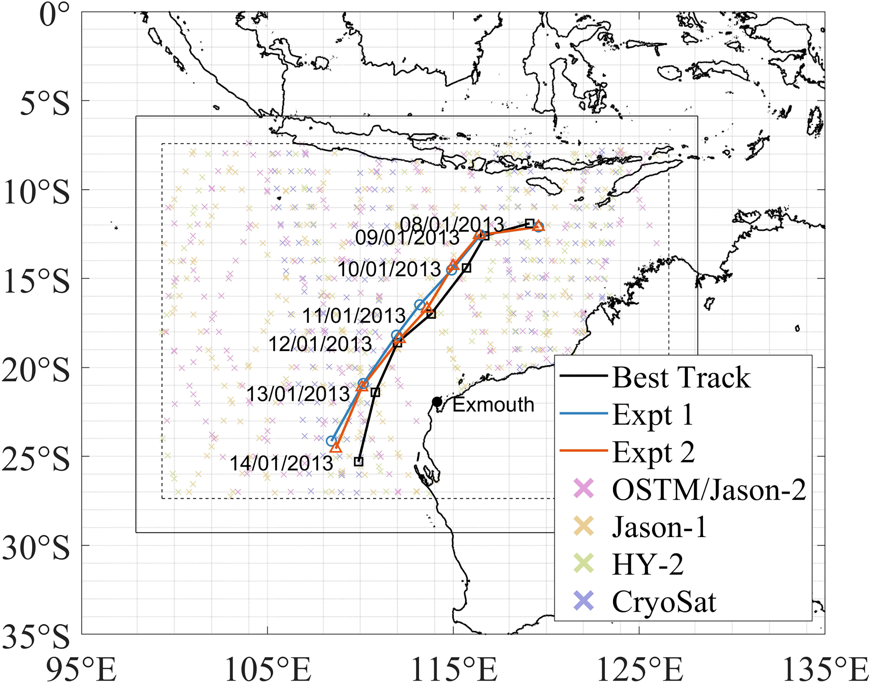
Figure 1 Domain of the COAWST model. The inner domain outlined by dashed lines (ROMS and SWAN) is nested with the outer domain outlined by solid lines (WRF). The best-track observations and the track of TC Narelle modeling without and with the spume scheme are represented in solid black lines with squares, solid blue lines with circles, and solid red lines with triangles, respectively. The passage points of satellites are represented by cross markers.

2.3 Experimental designs

The COAWST model was used to investigate the impact of spume on the modeling of TC Narelle. Historically, the Coupled Ocean-Atmosphere Response Experiment (COARE) bulk algorithm has been adopted to estimate air-sea interfacial HFs. Here, to characterize the role of spume in the air-sea heat exchange, we substituted the default bulk turbulent algorithm in the surface module within the WRF with the air-sea microphysical algorithm suggested by Andreas et al. (2008). In doing so and in accordance with Perrie (2004), spume-induced sensible and latent HFs were proportionally added to the interfacial direct air-sea sensible and latent HFs, respectively, as follows:

$\begin{array}{ll}{H}_{L,T}=H_L+H_{L,sp}& (5)\end{array}$

$\begin{array}{ll}{H}_{S,T}=H_S+H_{S,sp}& (6)\end{array}$

where $H_{L,T}$ and $H_{S,T}$ are the total latent and sensible heat transfer across the air-sea interface, respectively; $H_L$ and $H_s$ are the direct air-sea latent and sensible HFs, respectively; and $H_{L,sp}$ and $H_{S,sp}$ are the spume-induced latent and sensible HFs, respectively (see Supplementary Material 2 for more information). As such, by using the updated coupled model (i.e., Eqs. 1–6), two numerical experiments were conducted. Expt. 1 was the control run in which the spume scheme was absent, while Expt. 2 included the spume scheme. Therefore, the impact of spume (more specifically, spume produced by the bag-breakup mechanism, hereafter referred to as “the spume scheme”) on local atmospheric and oceanic environments can be investigated.

3 Results and discussion

3.1 Atmosphere

Figure 2 shows a comparison between observations from the International Best Track Archive for Climate Stewardship (IBTrACS) and the simulation results. The simulation results with and without the spume scheme are comparable before 06:00/10 January 2022; however, after 06:00/10 January 2022, the inclusion of the spume scheme deepens the minimum central pressure (P_min) by up to 20 hPa and significantly reduces the errors with observations. This improvement can also be seen in the maximum sustained surface wind speed (V_max). By introducing the spume scheme, V_max increases by up to 13 m s^-1 in contrast to the simulation without spume (Figure 2B), thus reducing the error with observations. While concurrent in situ observations are scarce due to the limitations of measurement techniques, we can observe improvements when comparing our simulated wind speeds at a 10-m height (U₁₀) to the measurements of ASCAT MetOp-A, CryoSat, HY-2, Jasson-1, and Ocean Surface Topography Mission/Jason-2 (Supplementary Material 3).

FIGURE 2

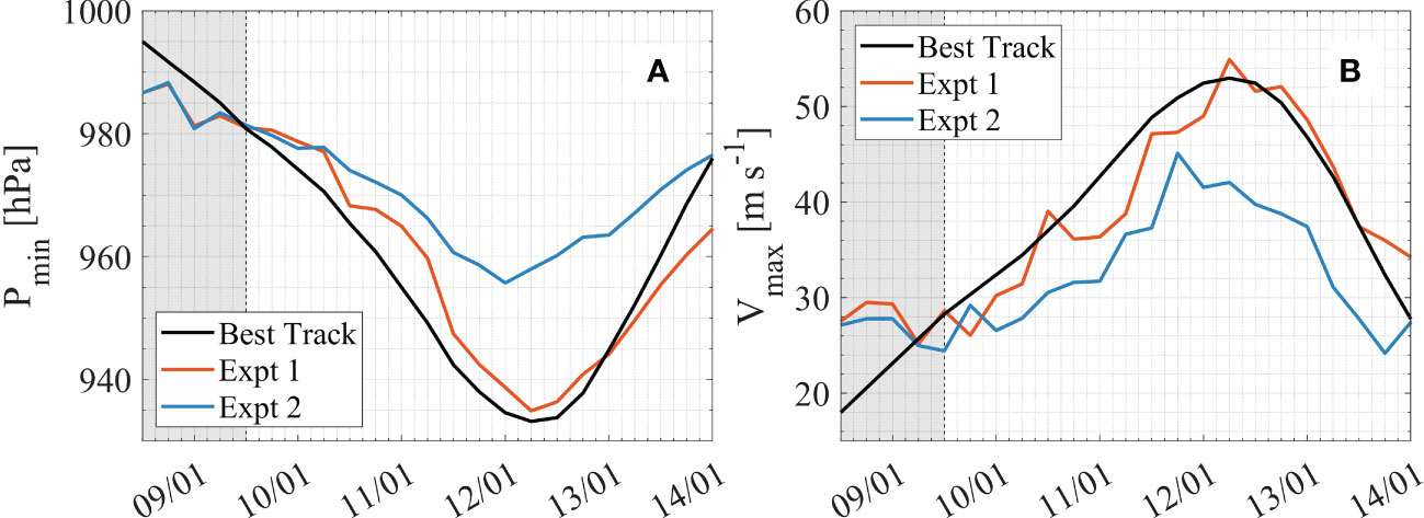
Figure 2 (A) Minimum central pressure (P_min) and (B) maximum sustained surface wind speed (V_max). The solid black line, solid blue line, and solid red line are the observations of the International Best Track Archive for Climate Stewardship and the modeling results without and with the spume scheme, respectively. The gray shadow represents the period of model spin-up.

Figures 3A, D, G present the spatial distributions of the total air-sea HFs of Expt. 1. The maximum of the HFs through the air-sea interfaces is located at the radius of maximum wind (RMW). Consistent with Expt. 1, the maximum of the HFs in Expt. 2 is at the RMW (Figures 3B, E, H). We observe that with the development and intensification of TC Narelle, the maximum of the HFs continuously increases. For example, the maximum of the HF azimuthal average reaches 450, 500, and 550 W m^-2 on 00:00/10 January 2013, 00:00/11 January 2013, and 00:00/12 January 2013, respectively. In comparison with Expt. 1, once the spume scheme is considered, the maximum HF azimuthal average is significantly enhanced by up to 150, 350, and 375 W m^-2 on 00:00/10 January 2013, 00:00/11 January 2013, and 00:00/12 January 2013, respectively (Figures 3C, F, I). This is because the seawater temperature and thus the initial temperature of the spume droplets are higher than the air that surrounds them, which means that the spume droplets are expected to transfer heat to the surrounding air. This, in turn, increases the quantity of heat transferred from the ocean to the above atmosphere. While spume is likely to cool the atmosphere because of evaporation, such a cooling process cannot be completed because of the limited suspension time of the spume in the air. This is consistent with the results of Andreas (1992) and Andreas et al. (2008), who proposed that the timescale of spume evaporation in the air (minutes to days) is much larger than that of the heat exchange resulting from temperature differences (seconds). While the spume-induced HFs are noticeable at RMW, spume has no discernible effect on the air-sea HFs in the areas located 120 km away from the center of the TC (Figures 3C, F, I). Therefore, we expect the structure of the TC to change considerably due to the presence of the sea spray spume.

FIGURE 3

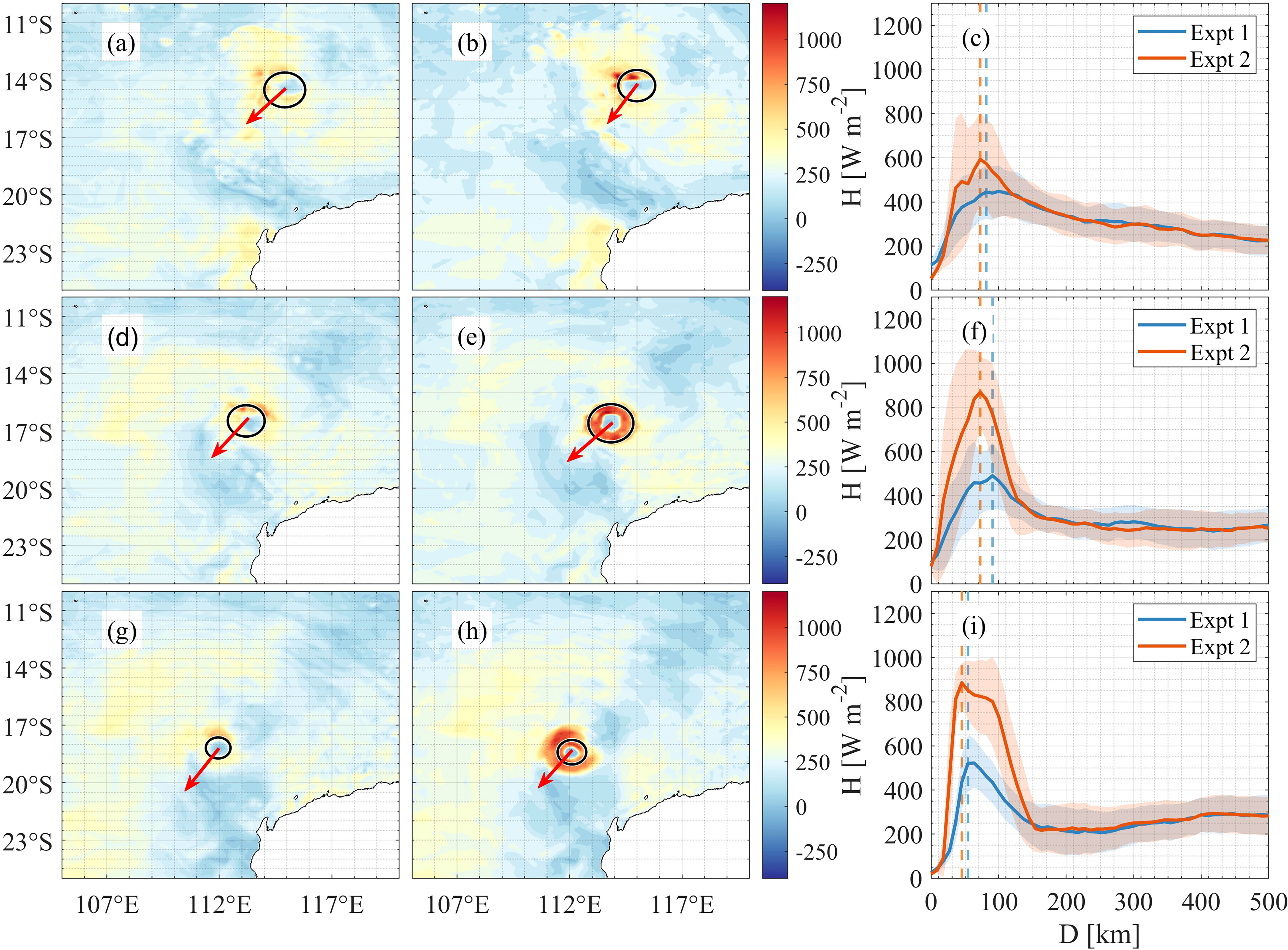
Figure 3 (A, D, G) are total air-sea heat fluxes without the spume scheme on 10–11 January 2013. (B, E, H) are the same as (A, D, G) but with the spume scheme. (C, F, I) represent the azimuthal averages of the total air-sea heat fluxes. The direction in which TC Narelle is moving forward at different times is demonstrated by the red arrows. The azimuthal averages of the total air-sea heat fluxes for the simulation results without and with the spume scheme are shown by solid blue and red lines, respectively. The standard deviations of the total air-sea heat fluxes in all radial directions are represented by shadows. The radius of maximum wind is represented by solid circles and dashed lines in spatial distributions and azimuthal averages, respectively.

Figures 4A, D, G depict the spatial distributions of the atmospheric pressure at various periods without the spume scheme. When compared to Expt. 2 (Figures 4B, E, H), we observe limited changes overall. However, the azimuthal averages of sea level pressure (SLP) are dramatically affected as a result of introducing the spume scheme, specifically within the RMW. For instance, in comparison with the simulation results of Expt. 1, Expt. 2 increases the minimum SLP azimuthal average by up to 2, 6, and 22 hPa on 00:00/10 January 2013, 00:00/11 January 2013, and 00:00/12 January 2013, respectively (Figures 4C, F, I).

FIGURE 4

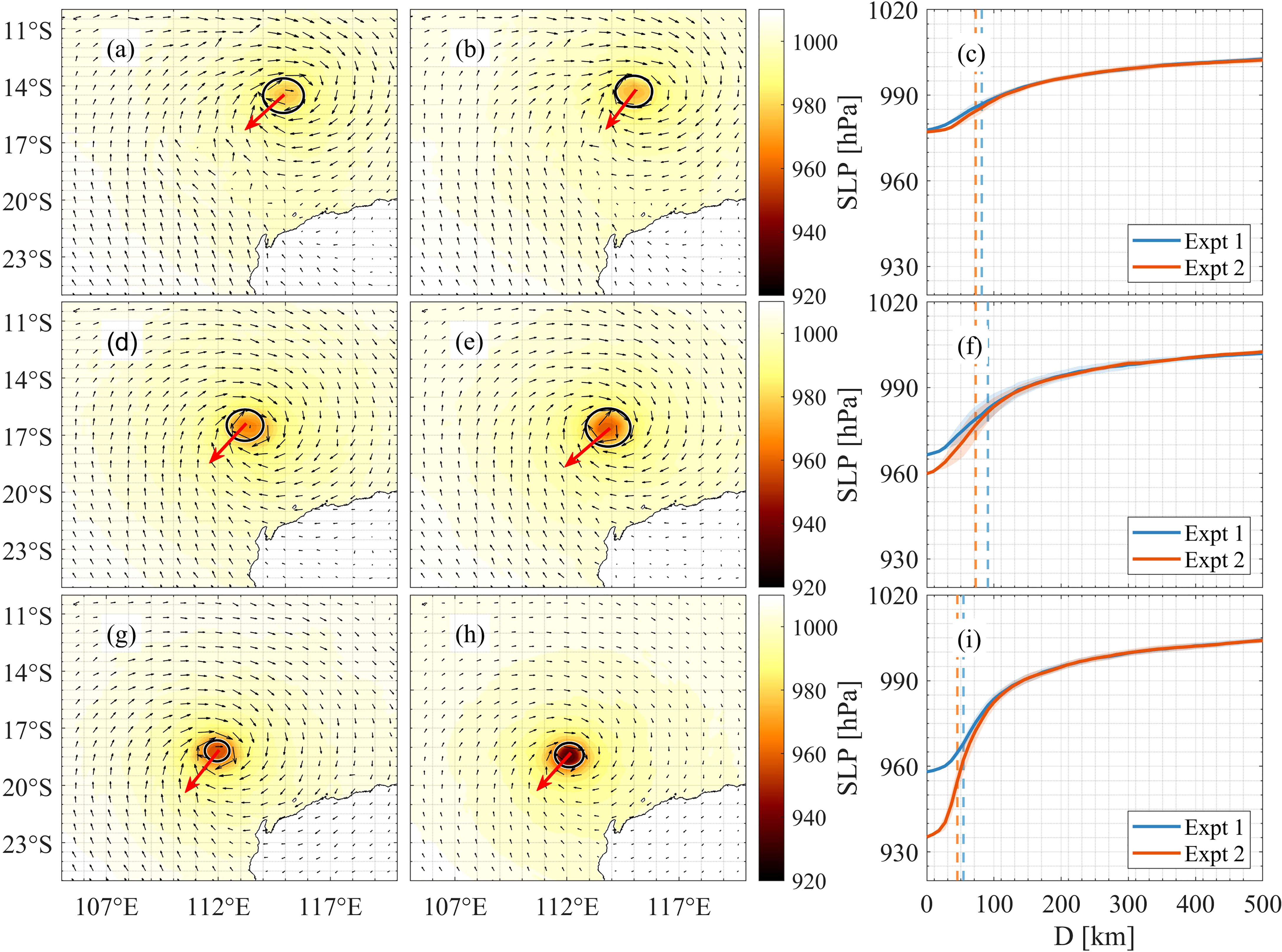
Figure 4 (A, D, G) are sea level pressure (SLP) without the spume scheme on 10–12 January 2013. (B, E, H) are the same as panels (A, D, G) but with the spume scheme. (C, F, I) represent the azimuthal averages of the SLP. The direction in which TC Narelle is moving forward at different times is demonstrated by the red arrows. The vectors are the directions of the local winds. The azimuthal averages of the SLP are shown by solid lines. The standard deviations of the SLP in all radial directions are represented by shadows. The radius of maximum wind is represented by solid circles and dashed lines in spatial distributions and azimuthal averages, respectively.

The spatial distribution of U₁₀ and the ocean surface stress at different times in Expt. 1 are shown in Figures 5A, D, G and Figures 6A, D, G, respectively. Once the spume effects are considered, while the directions of the local winds have slightly changed, the maximum U₁₀ and ocean surface stresses are greatly enhanced (Figures 5B, E, H; 6B, E, H). We notice that such an impact becomes more apparent with the development and intensification of the TC. This is in agreement with the spatial distributions of the HFs, which further show the impact of spume on the local wind fields. For example, in contrast with the simulation results without the spume scheme, adding spume increases the maximum of the U₁₀ azimuthal averages by up to 1.0, 6.6, and 22.9 m s^-1 and the maximum of the ocean surface stress azimuthal averages by up to 0.04, 0.80, and 1.61 N m^-2 on 00:00/10 January 2013, 00:00/11 January 2013, and 00:00/12 January 2013, respectively (Figures 5C, F, I; 6C, F, I). While the maximum of the U₁₀ is increased when introducing the spume, the location of the maximum U₁₀ moves closer to the TC center (i.e., the RMW decreases) such that the TC becomes smaller (on average 10 km) in comparison with the simulated results without the spume scheme.

FIGURE 5

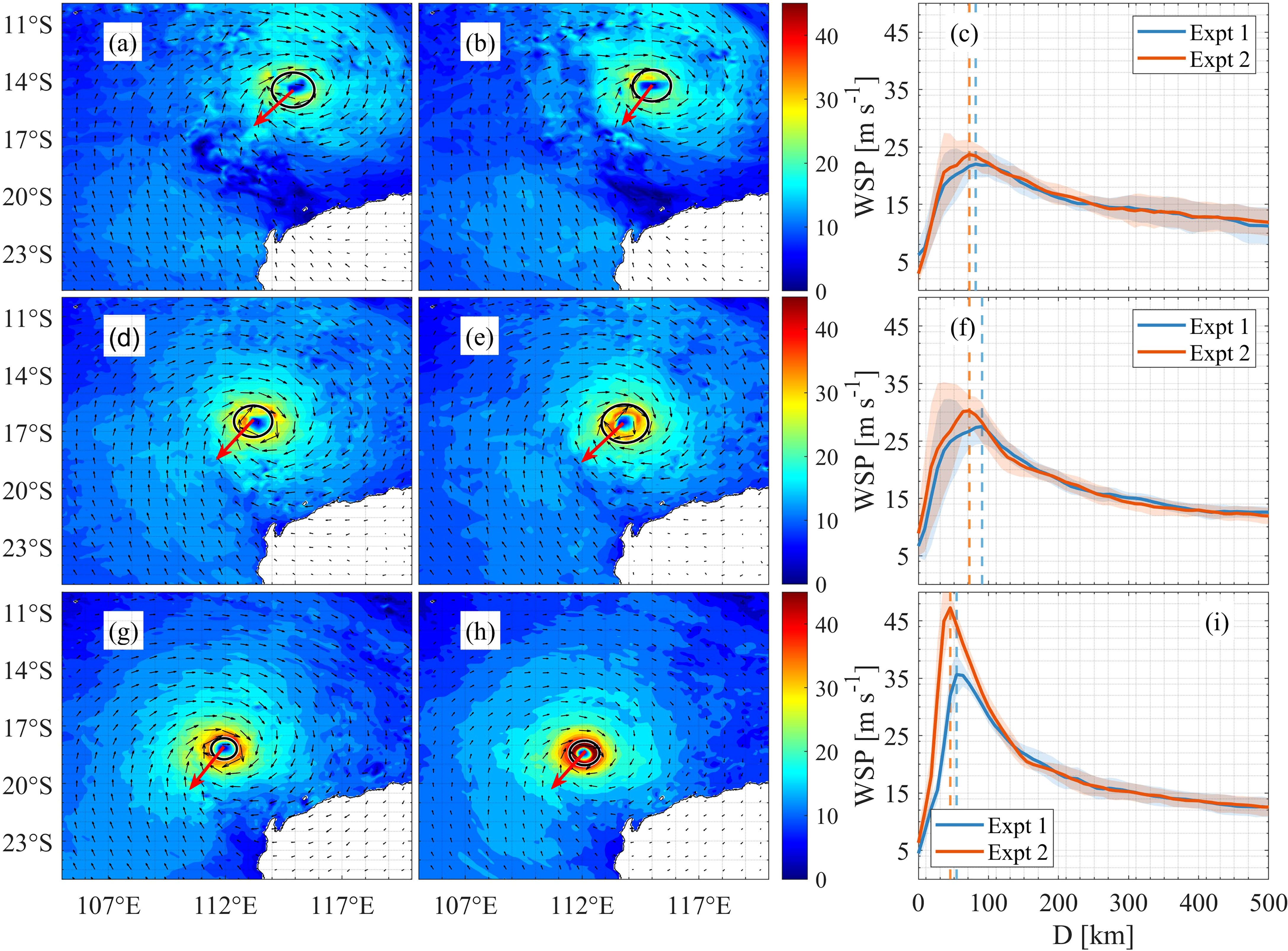
Figure 5 (A, D, G) are 10-m wind speed (U₁₀) without the spume scheme on 10–12 January 2013. (B, E, H) are the same as (A, D, G) but with the spume scheme. (C, F, I) represent the azimuthal averages of U₁₀. The direction in which TC Narelle is moving forward at different times is demonstrated by the red arrows. The vectors are the directions of the local winds. The azimuthal averages of U₁₀ are shown by solid lines. The standard deviations of U₁₀ in all radial directions are represented by shadows. The radius of maximum wind is represented by solid circles and dashed lines in spatial distributions and azimuthal averages, respectively.

FIGURE 6

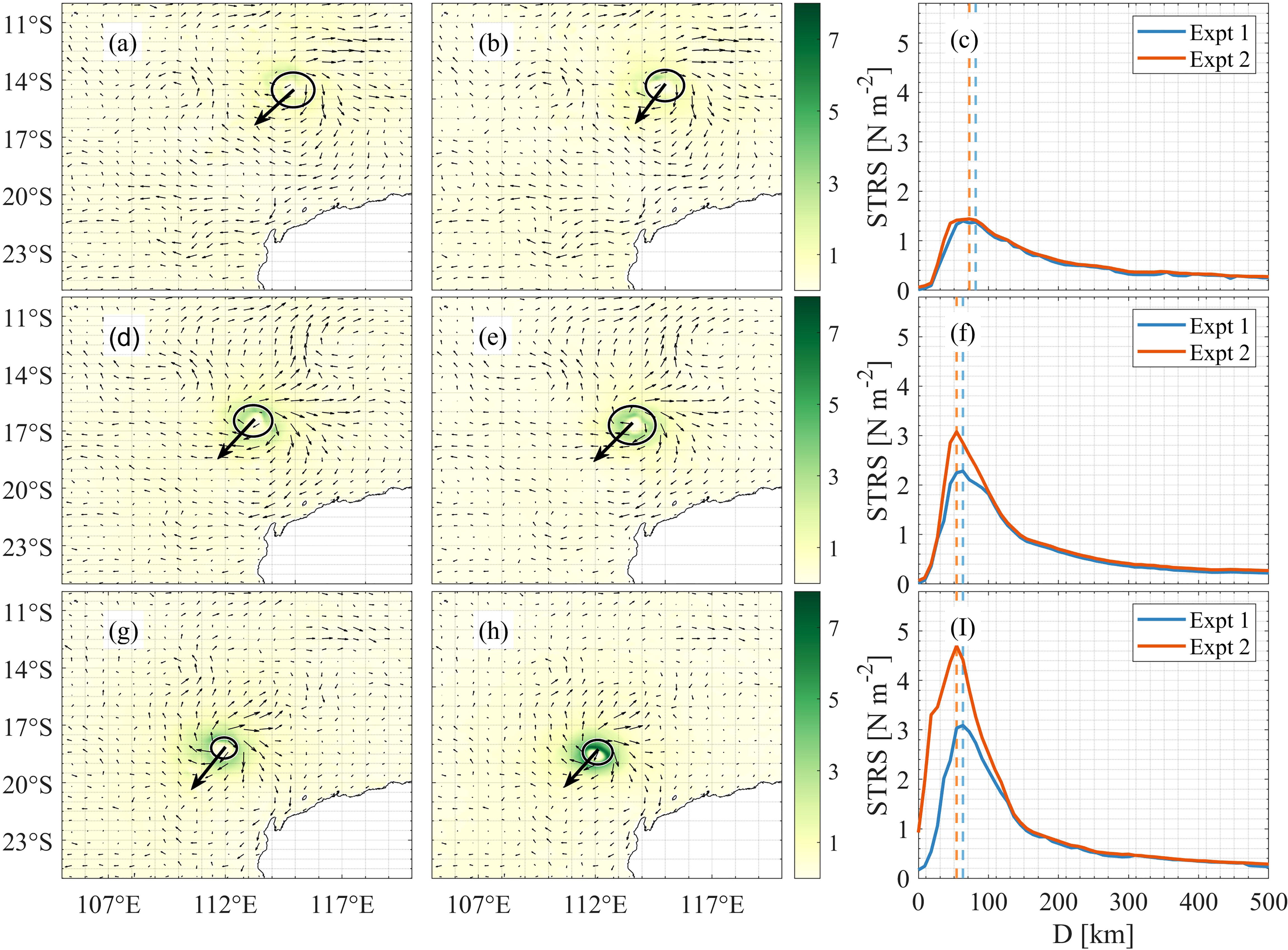
Figure 6 (A, D, G) are ocean surface stress without the spume scheme on 10–12 January 2013. (B, E, H) are the same as (A, D, G) but with the spume scheme. (C, F, I) represent the azimuthal averages of surface stress. The direction in which TC Narelle is moving forward at different times is demonstrated by the red arrows. The vectors are the directions of the local currents. The azimuthal maximum of the surface stress is shown by solid lines. The radius of maximum wind is represented by solid circles and dashed lines in spatial distributions and azimuthal averages, respectively.

3.2 Waves

During the passage of the TC, we expect spume to make a significant impact on the waves as spume radically affects wind fields, and the local sea state is highly dependent upon these fields. Figures 7A, B, D, E, G, H depict the spatial distributions of significant wave height (Hs) at different times for Expt. 1 and Expt. 2, respectively. The maximum Hs is largely increased because of the adoption of the scheme in Expt. 2. This increment, consistent with the development of U₁₀, increases with the intensification of the TC. Specifically, the maximum Hs of Expt. 2 is enhanced by up to 1.3, 1.4, and 3.8 m on 00:00/10 January 2013, 00:00/11 January 2013, and 00:00/12 January 2013, respectively (Figures 7C, F, I) as compared to the simulated results in Expt. 1. We note that the simulation results for Hs are improved when introducing spume as compared with the measurements of CryoSat, HY-2, Jason-1, and Ocean Surface Topography Mission/Jason-2 (Supplementary Material 3). While spume produces critical effects on Hs, it negligibly alters the location where the maximum Hs occurs (i.e., the maximum Hs distributes averagely in all radial directions). As TC Narelle occurred in the Southern Hemisphere, the maximum Hs is expected to be located in the left front quadrant of the TC’s forward direction. This is due to the fact that a (young) swell propagates in the same direction as the locally generated wind sea, which is in the left front as a TC spins clockwise in the Southern Hemisphere, whereas the propagation directions of the wind sea and (young) swells keep opposite and/or cross each other (Holthuijsen et al., 2012). This spatial distribution pattern is not observed in either Expt. 1 or Expt. 2. One possible reason is that the movement speed of TC Narelle is so slow in the experiments that the waves under the TC system are largely dominated by the locally generated wind waves instead of the swell produced at earlier points (Moon et al., 2003).

FIGURE 7

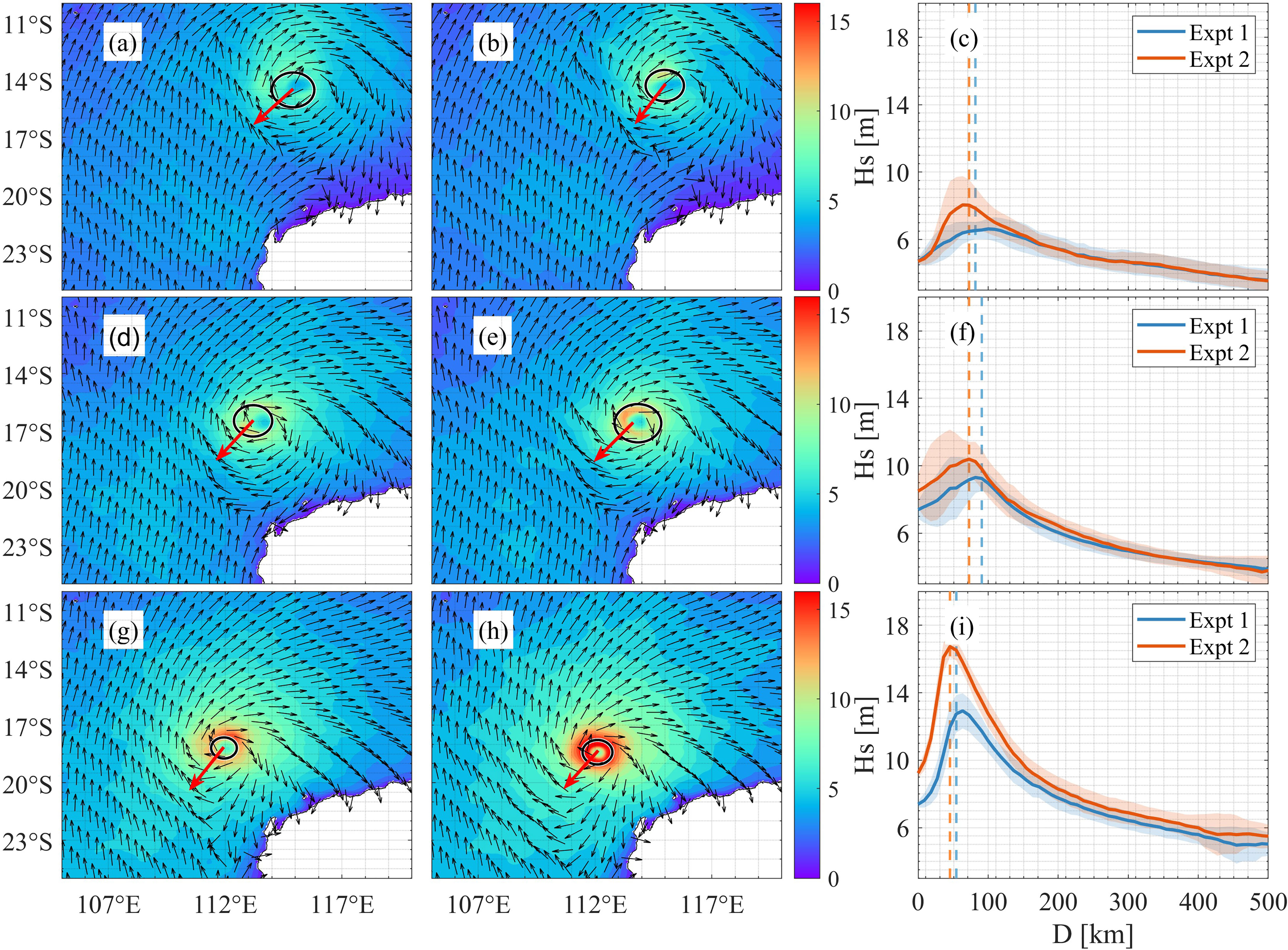
Figure 7 (A, D, G) are significant wave height (Hs) without the spume scheme on 10–12 January 2013. (B, E, H) are the same as (A, D, G) but with the spume scheme. (C, F, I) represent the azimuthal averages of Hs. The direction in which TC Narelle is moving forward at different times is demonstrated by the red arrows. The vectors are the propagation directions of the local waves. The azimuthal averages of Hs are shown by solid lines. The standard deviations of Hs in all radial directions are represented by shadows. The radius of maximum wind is represented by solid circles and dashed lines in spatial distributions and azimuthal averages, respectively.

3.3 Ocean

As the underlying ocean is closely coupled with atmospheric environments and local wave fields, and spume significantly alters the atmosphere and waves, we can expect a controlling impact of spume on the upper ocean. Figures 8A, D, G show the spatial distributions of sea surface temperature (SST). During the passage of the TC system, the SST decreases as a result of deep and cold water rising to the ocean surface as a consequence of upwelling and turbulent mixing. It can be seen that the SST decrease caused by the TC system occurs in the back quadrants of the TC as it moves forward, and the extent of the SST decrease follows the intensity of the TC system. As compared with the simulation results in Expt. 1, incorporating the spume scheme has negligible effects on the direction of the ocean current, but it enhances the extent and expands the area of decreasing SST (Figures 8B, E, H). For example, while the azimuthal average of the minimum SST in Expt. 2 is equivalent to that in Expt. 1 on both 00:00/10 January 2013 and 00:00/11 January 2013, the decline in SST is largely more pronounced in Expt. 2 on 00:00/12 January 2013 (Figures 8C, F, I). That is, the minimum SST is further decreased by 1.2°C in Expt. 2 as compared to that in Expt. 1 mainly at the RMW. This is in accordance with current studies suggesting that spume strengthens the SST cooling caused by a TC system (Perrie, 2004; Perrie et al., 2005; Xu et al., 2022), which is a direct result of the spume-induced intensification of the TC system. This can be explained as follows. Spume increases total air-sea HFs, reinforcing the local winds and waves specifically at the RMW. In turn, additional turbulent kinetic energy from the atmosphere to the ocean is provided, enhancing warm surface water mixing with cooler water from the surface to the thermocline and promoting the upwelling of colder water to the surface. Once the SST cooling has become enhanced because of the strong upwelling, the temperature of the spume is also reduced, leading to a reduction in spume-induced HFs, providing negative feedback on the interaction between the spume and the upper ocean.

FIGURE 8

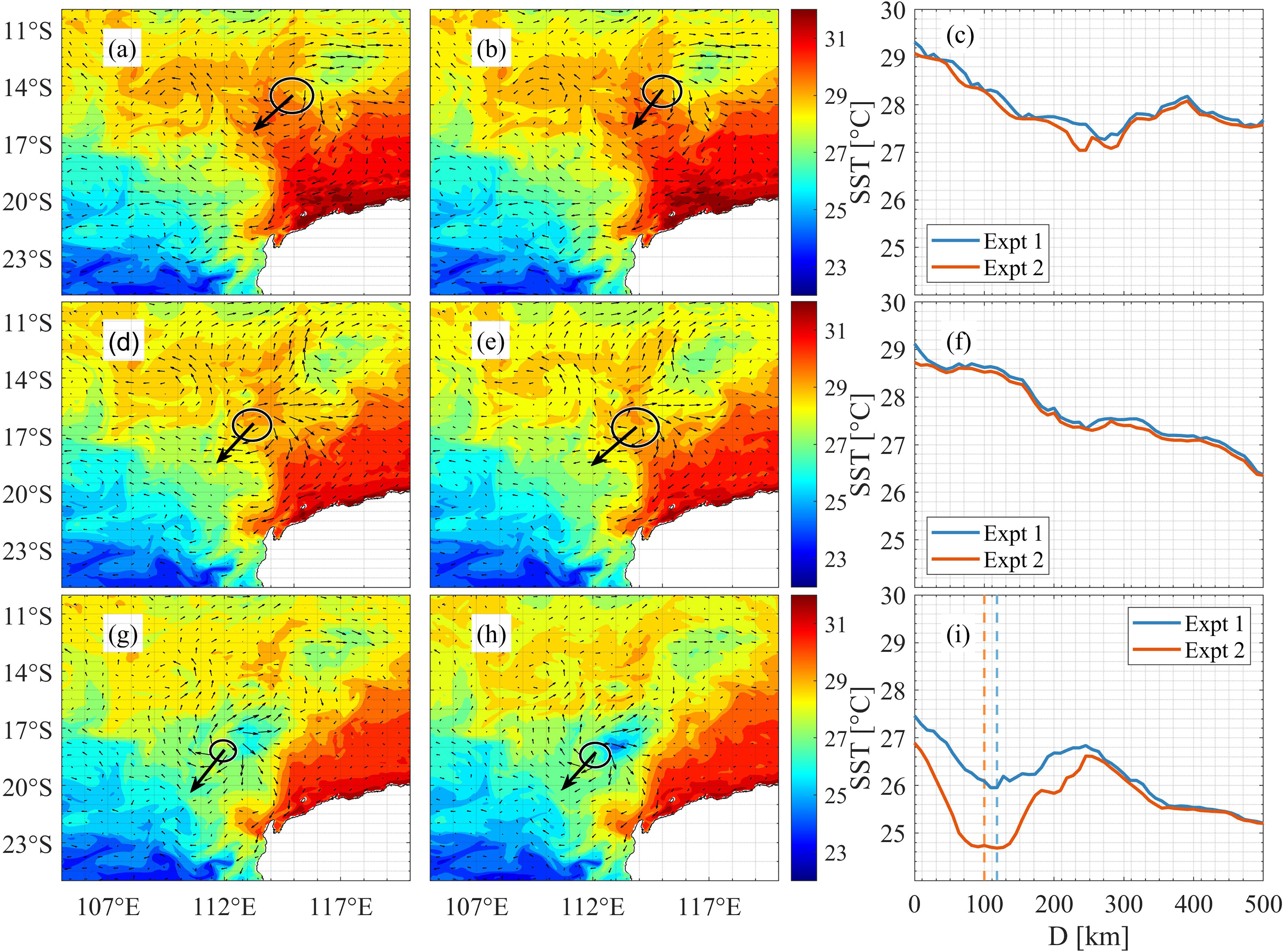
Figure 8 (A, D, G) are sea surface temperature (SST) without the spume scheme on 10–12 January 2013. (B, E, H) are the same as (A, D, G) but with the spume scheme. (C, F, I) represent the azimuthal averages of SST. The direction in which TC Narelle is moving forward at different times is demonstrated by the red arrows. The vectors are the directions of the local currents. The azimuthal minimum of SST is shown by solid lines. The radius of maximum wind is represented by solid circles and dashed lines in spatial distributions and azimuthal averages, respectively.

4 Conclusion

The present study used a coupled atmosphere-ocean-wave numerical model to investigate the impact of a bag breakup–induced spume scheme on the atmosphere, ocean, and wave modeling of the passage of TC Narelle. We did so by extending an air-sea turbulent bulk algorithm by implementing an observation-based spume parameterization. Two different numerical experiments were performed, one without and one with the spume scheme, to study the impact of spume on the air-sea interactions during TC Narelle.

When considering our simulations, we can observe substantial improvements in the ability to model minimum SLP and maximum wind speed as compared with observations from the World Meteorology Organization. These improvements are consistent with observations from ASCAT MetOp-A and Ocean Surface Topography Mission/Jason-2. By providing additional heat to the atmosphere, spume causes a TC system to intensify, and this is represented in our model by a decrease in P_min and an increase in V_max. Furthermore, as U₁₀ increases, RMW reduces by approximately 10 km in the model, suggesting a complex but critical impact of spume on the intensity, structure, and size of the TC system.

It can also be noticed that the stronger prevailing winds induced by spume ultimately contribute to higher sea states, and we can observe an increase in Hs by up to 3.8 m. Since the generation of spume is heavily influenced by the interaction between local waves and winds, an increase in U₁₀ and rise in Hs can result in a positive feedback on spume production. In contrast with the positive feedback between the spume and local winds and waves, a negative feedback can occur between the spume and the upper ocean. This happens because the intensification of the TC system when including spume leads to stronger vertical mixing and upwelling, which in turn enhance SST cooling after the TC passes. For instance, we can see a decrease in the minimum SST by as much as 1.2°C in our simulations. Enhanced SST cooling can reduce the impact of spume on air-sea HFs by reducing the temperature difference between the ocean (and thus spume droplets) and the atmosphere. Therefore, it can be seen that spume has significant effects on atmospheric and oceanic environments by modulating wind speed, Hs, and SST. Therefore, spume must be included in operational models for TC forecasting.

Data availability statement

The original contributions presented in the study are included in the article/Supplementary Material. Further inquiries can be directed to the corresponding author.

Author contributions

All authors contribute to this present work and approve the submitted version. XX designed and conducted the numerical simulations. XX initiated the first version of the manuscript. JV, TW, I-JM, QL, and AB contributed to the final revision of the manuscript. All authors contributed to the article and approved the submitted version.

Funding

XX, JV, and AB acknowledge the support of the Centre of Disaster Management and Public Safety of the University of Melbourne. AB acknowledges support of the US Office of Naval Research Global, Grant Number N62909-20-1-2080. I-JM was supported by Korea Institute of Marine Science & Technology Promotion (KIMST) funded by the Ministry of Oceans and Fisheries (20210607, "Establishment of the ocean research station in the jurisdiction zone and convergence research"; 20220566, "Study on Northwestern Pacific Warming and Genesis and Rapid Intensification of Typhoon”).

Conflict of interest

The authors declare that the research was conducted in the absence of any commercial or financial relationships that could be construed as a potential conflict of interest.

Publisher’s note

All claims expressed in this article are solely those of the authors and do not necessarily represent those of their affiliated organizations, or those of the publisher, the editors and the reviewers. Any product that may be evaluated in this article, or claim that may be made by its manufacturer, is not guaranteed or endorsed by the publisher.

Supplementary material

The Supplementary Material for this article can be found online at: https://www.frontiersin.org/articles/10.3389/fmars.2023.1133149/full#supplementary-material

References

Andreas E. L. (1992). Sea Spray and the turbulent air-Sea heat fluxes. J. Geophys Res. 97 (C7), 11429–11441. doi: 10.1029/92jc00876

CrossRef Full Text | Google Scholar

Andreas E. L., Emanuel K. A. (2001). Effects of sea spray on tropical cyclone intensity. J. atmospheric Sci. 58 (24), 3741–3751. doi: 10.1175/1520-0469(2001)058<3741:EOSSOT>2.0.CO;2

CrossRef Full Text | Google Scholar

Andreas E. L., Persson P. O. G., Hare J. E. (2008). A bulk turbulent air–sea flux algorithm for high-wind, spray conditions. J. Phys. Oceanogr 38 (7), 1581–1596. doi: 10.1175/2007JPO3813.1

CrossRef Full Text | Google Scholar

Chan J. C. (1985). Tropical cyclone activity in the northwest pacific in relation to the El Niño/Southern oscillation phenomenon. Monthly weather Rev. 113 (4), 599–606. doi: 10.1175/1520-0493(1985)113<0599:TCAITN>2.0.CO;2

CrossRef Full Text | Google Scholar

Chan J. C., Kepert J. D. (2010). Global perspectives on tropical cyclones: from science to mitigation World Scientific. doi: 10.1142/7597

CrossRef Full Text | Google Scholar

Chen S.-H., Sun W.-Y. (2002). A one-dimensional time dependent cloud model. J. Meteorol Soc. Japan. Ser. II 80 (1), 99–118. doi: 10.2151/jmsj.80.99

CrossRef Full Text | Google Scholar

Dudhia J. (1989). Numerical study of convection observed during the winter monsoon experiment using a mesoscale two-dimensional model. J. Atmospheric Sci. 46 (20), 3077–3107. doi: 10.1175/1520-0469(1989)046<3077:NSOCOD>2.0.CO;2

CrossRef Full Text | Google Scholar

Dudhia J. (1996). A multi-layer soil temperature model for MM5[C]//Preprints, The Sixth PSU/NCAR mesoscale model users’ workshop. Boulder, CO, USA: National Center for Atmospheric Research, 22–24. Available at: https://scholar.google.co.jp/scholar?hl=zh-CN&as_sdt=0%2C5&as_vis=1&q=A+multi-layer+soil+temperature+model+for+MM5+J+Dudhia&btnG=

Google Scholar

Emanuel K. (2018). 100 years of progress in tropical cyclone research. Meteorol Monogr. 59, 15.11–15.68. doi: 10.1175/AMSMONOGRAPHS-D-18-0016.1

CrossRef Full Text | Google Scholar

Emanuel K., DesAutels C., Holloway C., Korty R. (2004). Environmental control of tropical cyclone intensity. J. Atmospheric Sci. 61 (7), 843–858. doi: 10.1175/1520-0469(2004)061<0843:Ecotci>2.0.Co;2

CrossRef Full Text | Google Scholar

Holthuijsen L. H., Powell M. D., Pietrzak J. D. (2012). Wind and waves in extreme hurricanes. J. Geophys Research: Oceans 117 (C9). doi: 10.1029/2012jc007983

CrossRef Full Text | Google Scholar

Kepert J. D. (2010). Tropical cyclone structure and dynamics. Global Perspect. Trop. cyclones: Sci. to mitigation 2010, 3–53. doi: 10.1142/9789814293488_0001

CrossRef Full Text | Google Scholar

Koga M. (1981). Direct production of droplets from breaking wind-waves–its observation by a multi-colored overlapping exposure photographing technique. Tellus 33 (6), 552–563. doi: 10.1111/j.2153-3490.1981.tb01781.x

CrossRef Full Text | Google Scholar

Komen G., Hasselmann S., Hasselmann K. (1984). On the existence of a fully developed wind-sea spectrum. J. Phys. oceanogr 14 (8), 1271–1285. doi: 10.1175/1520-0485(1984)014<1271:OTEOAF>2.0.CO;2

CrossRef Full Text | Google Scholar

Lhuissier H., Villermaux E. (2012). Bursting bubble aerosols. J. Fluid Mechanics 696, 5–44. doi: 10.1017/jfm.2011.418

CrossRef Full Text | Google Scholar

Mehta S., Ortiz-Suslow D. G., Smith A. W., Haus B. K. (2019). A laboratory investigation of spume generation in high winds for fresh and seawater. J. Geophys Research: Atmospheres 124 (21), 11297–11312. doi: 10.1029/2019JD030928

CrossRef Full Text | Google Scholar

Mlawer E. J., Taubman S. J., Brown P. D., Iacono M. J., Clough S. A. (1997). Radiative transfer for inhomogeneous atmospheres: RRTM, a validated correlated-k model for the longwave. J. Geophys Research: Atmospheres 102 (D14), 16663–16682. doi: 10.1029/97JD00237

CrossRef Full Text | Google Scholar

Moon I.-J., Ginis I., Hara T. (2004a). Effect of surface waves on air–Sea momentum exchange. part II: behavior of drag coefficient under tropical cyclones. J. Atmospheric Sci. 61 (19), 2334–2348. doi: 10.1175/1520-0469(2004)061<2334:Eoswoa>2.0.Co;2

CrossRef Full Text | Google Scholar

Moon I.-J., Ginis I., Hara T., Thomas B. (2007). A physics-based parameterization of air–Sea momentum flux at high wind speeds and its impact on hurricane intensity predictions. Monthly Weather Rev. 135 (8), 2869–2878. doi: 10.1175/mwr3432.1

CrossRef Full Text | Google Scholar

Moon I.-J., Ginis I., Hara T., Tolman H. L., Wright C. W., Walsh E. J. (2003). Numerical simulation of Sea surface directional wave spectra under hurricane wind forcing. J. Phys. Oceanogr 33 (8), 1680–1706. doi: 10.1175/1520-0485(2003)033<1680:Nsossd>2.0.Co;2

CrossRef Full Text | Google Scholar

Moon I.-J., Hara T., Ginis I., Belcher S. E., Tolman H. L. (2004b). Effect of surface waves on air–Sea momentum exchange. part I: effect of mature and growing seas. J. Atmospheric Sci. 61 (19), 2321–2333. doi: 10.1175/1520-0469(2004)061<2321:Eoswoa>2.0.Co;2

CrossRef Full Text | Google Scholar

Nakanishi M., Niino H. (2006). An improved Mellor–Yamada level-3 model: Its numerical stability and application to a regional prediction of advection fog. Boundary Layer Meteorol. 119, 397–407.

Google Scholar

Nakanishi M., Niino H. (2009). Development of an improved turbulence closure model for the atmospheric boundary layer. J Meteorol. Soc. Japan. Ser. II 87 (5), 895–912.

Google Scholar

Nordhaus W. D. (2010). The economics of hurricanes and implications of global warming. Climate Change Economics 1 (01), 1–20. doi: 10.1142/S2010007810000054

CrossRef Full Text | Google Scholar

Ortiz-Suslow D. G., Haus B. K., Mehta S., Laxague N. J. M. (2016). Sea Spray generation in very high winds. J. Atmospheric Sci. 73 (10), 3975–3995. doi: 10.1175/jas-d-15-0249.1

CrossRef Full Text | Google Scholar

Perrie W. (2004). Simulation of extratropical hurricane Gustav using a coupled atmosphere-ocean-sea spray model. Geophys Res. Lett. 31 (3). doi: 10.1029/2003gl018571

CrossRef Full Text | Google Scholar

Perrie W., Zhang W., Andreas E. L., Li W., Gyakum J., McTaggart-Cowan R. (2005). Sea Spray impacts on intensifying midlatitude cyclones. J. Atmospheric Sci. 62 (6), 1867–1883. doi: 10.1175/JAS3436.1

CrossRef Full Text | Google Scholar

Pruppacher H. R., Klett J. D. (1978). “Hydrodynamics of single cloud and precipitation particles,” in Microphysics of clouds and precipitation (Springer), 282–346. Available at: https://scholar.google.com.au/scholar?hl=zh-CN&as_sdt=0%2C5&q=Hydrodynamics+of+single+cloud+and+precipitation+particles&btnG=#d=gs_cit&t=1682405828272&u=%2Fscholar%3Fq%3Dinfo%3Afj53TOum7gkJ%3Ascholar.google.com%2F%26output%3Dcite%26scirp%3D0%26hl%3Dzh-CN

Google Scholar

Rizza U., Canepa E., Miglietta M. M., Passerini G., Morichetti M., Mancinelli E., et al. (2021). Evaluation of drag coefficients under medicane conditions: coupling waves, sea spray and surface friction. Atmospheric Res. 247, 105207. doi: 10.1016/j.atmosres.2020.105207

CrossRef Full Text | Google Scholar

Rizza U., Canepa E., Ricchi A., Bonaldo D., Carniel S., Morichetti M., et al. (2018). Influence of wave state and sea spray on the roughness length: feedback on medicanes. Atmosphere 9 (8), 301. doi: 10.3390/atmos9080301

CrossRef Full Text | Google Scholar

Shchepetkin A. F., McWilliams J. C. (2005). The regional oceanic modeling system (ROMS): a split-explicit, free-surface, topography-following-coordinate oceanic model. Ocean Model. 9 (4), 347–404. doi: 10.1016/j.ocemod.2004.08.002

CrossRef Full Text | Google Scholar

Skamarock W. C., Klemp J. B. (2008). A time-split nonhydrostatic atmospheric model for weather research and forecasting applications. J. Comput. Phys. 227 (7), 3465–3485. doi: 10.1016/j.jcp.2007.01.037

CrossRef Full Text | Google Scholar

Smith R. K., Montgomery M. T., Kilroy G., Tang S. (2015). Tropical low formation during the Australian monsoon: the events of January 2013. Aust. Meteorol Oceanographic J. 65 (4), 318–341. doi: 10.22499/2.6503.003

CrossRef Full Text | Google Scholar

Southern R. (1979). The global socio-economic impact of tropical cyclones. Aust. Meteorol Magazine 1979, 175–195.

Google Scholar

Spiel D. E. (1998). On the births of film drops from bubbles bursting on seawater surfaces. J. Geophys Research: Oceans 103 (C11), 24907–24918. doi: 10.1029/98JC02233

CrossRef Full Text | Google Scholar

Spiel D. E., De Leeuw G. (1996). Formation and production of sea spray aerosol. J. Aerosol Sci. 27, S65–S66. doi: 10.1016/0021-8502(96)00105-X

CrossRef Full Text | Google Scholar

Strachan J., Vidale P. L., Hodges K., Roberts M., Demory M.-E. (2013). Investigating global tropical cyclone activity with a hierarchy of AGCMs: the role of model resolution. J. Climate 26 (1), 133–152. doi: 10.1175/jcli-d-12-00012.1

CrossRef Full Text | Google Scholar

Troitskaya Y., Druzhinin O., Kozlov D., Zilitinkevich S. (2018a). The “Bag breakup” spume droplet generation mechanism at high winds. part II: contribution to momentum and enthalpy transfer. J. Phys. Oceanogr 48 (9), 2189–2207. doi: 10.1175/jpo-d-17-0105.1

CrossRef Full Text | Google Scholar

Troitskaya Y., Kandaurov A., Ermakova O., Kozlov D., Sergeev D., Zilitinkevich S. (2017). Bag-breakup fragmentation as the dominant mechanism of sea-spray production in high winds. Sci. Rep. 7 (1), 1–4. doi: 10.1038/s41598-017-01673-9

PubMed Abstract | CrossRef Full Text | Google Scholar

Troitskaya Y., Kandaurov A., Ermakova O., Kozlov D., Sergeev D., Zilitinkevich S. (2018b). The “Bag breakup” spume droplet generation mechanism at high winds. part I: spray generation function. J. Phys. Oceanogr 48 (9), 2167–2188. doi: 10.1175/jpo-d-17-0104.1

CrossRef Full Text | Google Scholar

Veron F., Hopkins C., Harrison E. L., Mueller J. A. (2012). Sea Spray spume droplet production in high wind speeds. Geophys Res. Lett. 39 (16), n/a–n/a. doi: 10.1029/2012gl052603

CrossRef Full Text | Google Scholar

Vigdor J. (2008). The economic aftermath of hurricane Katrina. J. Economic Perspect. 22 (4), 135–154. doi: 10.1257/jep.22.4.135

CrossRef Full Text | Google Scholar

Warner J. C., Armstrong B., He R., Zambon J. B. (2010a). Development of a coupled ocean–Atmosphere–Wave–Sediment transport (COAWST) modeling system. Ocean Model. 35 (3), 230–244. doi: 10.1016/j.ocemod.2010.07.010

CrossRef Full Text | Google Scholar

Warner J. C., Rockwell Geyer W., Arango H. G. (2010b). Using a composite grid approach in a complex coastal domain to estimate estuarine residence time. Comput. Geosciences 36 (7), 921–935. doi: 10.1016/j.cageo.2009.11.008

CrossRef Full Text | Google Scholar

White C. J., Fox-Hughes P. (2013). Seasonal climate summary southern hemisphere (summer 2012-13): australia's hottest summer on record and extreme east coast rainfall. Aust. Meteorol Oceanographic J. 63 (3), 443–456. doi: 10.1071/ES13033

CrossRef Full Text | Google Scholar

Wu R., Zhang H., Chen D., Li C., Lin J. (2018). Impact of typhoon kalmaegi, (2014) on the south China Sea: simulations using a fully coupled atmosphere-ocean-wave model. Ocean Model. 131, 132–151. doi: 10.1016/j.ocemod.2018.08.004

CrossRef Full Text | Google Scholar

Xu X., Voermans J. J., Liu Q., Moon I.-J., Guan C., Babanin A. V. (2021a). Impacts of the wave-dependent Sea spray parameterizations on air–Sea–Wave coupled modeling under an idealized tropical cyclone. J. Mar. Sci. Eng. 9 (12), 1390. doi: 10.3390/jmse9121390

CrossRef Full Text | Google Scholar

Xu X., Voermans J. J., Ma H., Guan C., Babanin A. V. (2021b). A wind-wave-dependent sea spray volume flux model based on field experiments. J. Mar. Sci. Eng. 9 (11), 1168. doi: 10.3390/jmse9111168

CrossRef Full Text | Google Scholar

Xu X., Voermans J. J., Moon I. J., Liu Q., Guan C., Babanin A. V. (2022). Sea Spray impacts on tropical cyclone olwyn using a coupled atmosphere-Ocean-Wave model. J. Geophys Research: Oceans 127 (8), e2022JC018557. doi: 10.1029/2022JC018557

CrossRef Full Text | Google Scholar

Zhang L., Zhang X., Chu P. C., Guan C., Fu H., Chao G., et al. (2017). Impact of sea spray on the yellow and East China seas thermal structure during the passage of typhoon rammasun, (2002). J. Geophys Research: Oceans 122 (10), 7783–7802. doi: 10.1002/2016jc012592

CrossRef Full Text | Google Scholar

Zhang L., Zhang X., Perrie W., Guan C., Dan B., Sun C., et al. (2021). Impact of Sea spray and Sea surface roughness on the upper ocean response to super typhoon haitang, (2005). J. Phys. Oceanogr. 51 (6), 1929–1945. doi: 10.1175/jpo-d-20-0208.1

CrossRef Full Text | Google Scholar