MCSTNet: a memory-contextual spatiotemporal transfer network for prediction of SST sequences and fronts with remote sensing data

1 Introduction

Comprehending complex ocean phenomena is a difficult task since plenty of natural processes must be taken into account. Numerical models based on physical equations have long been used in the field of ocean phenomena prediction. In-depth research is made possible due to the abundance of ocean products that are derived from satellites, which also emphasizes the need for practical techniques for researching time-series observations. As one of the most time-honored ocean products, sea surface temperature (SST) is a key factor in helping to comprehend scientific issues concerning sea-air interaction, biological, chemical, and physical oceanography. SST is frequently applied to disclose a variety of important ocean phenomena, such as ocean fronts (Legeckis, 1977). When dealing with phenomena of a complex nature, traditional statistical analysis approaches are restricted by their shallow model structure.

Deep neural networks (DNNs) are an upgraded version of artificial neural networks (ANNs) that are one of the most widely used and currently prominent deep learning (DL) approaches, which use valid parameter optimization techniques and architecture designs (Jordan and Mitchell, 2015; LeCun et al., 2015). Compared to conventional statistical models, DL approaches are far more sophisticated. They have been widely applied in oceanography domains (Ducournau and Fablet, 2016; Ham et al., 2019; Reichstein et al., 2019; Li et al., 2020; Buongiorno Nardelli et al., 2022). It is efficient to discover and mine the complex rules in a time series of large amounts of remote sensing data (Zheng et al., 2020; Liu et al., 2021). Inspired by the video frame prediction using DL approaches (Wang et al., 2021; Gao et al., 2022), in this paper, we develop an SST pattern prediction method by building a DL model.

There are many different algorithms for DL, two typical ones of them being convolutional neural networks (CNNs) (Kunihiko and Sei, 1982) and recurrent neural networks (RNNs) (Glorot et al., 2011). CNNs are generally used in computer vision and are essentially input-to-output mappings that learn a large number of mapping relationships between inputs and outputs. On the other hand, RNNs are commonly applied in natural language processing (NLP) and various sequence processing tasks, where information is passed through repetitive loops so that the network can remember the sequence information and analyze patterns of data variation across the sequence.

The improvements in the structures of RNN, such as long short-term memory (LSTM), have better memory capability and long-term dependency to handle sequence prediction problems. While traditional RNN structures suffer from vanishing and exploding gradients when dealing with long sequences, resulting in ineffective information transfer. LSTM enhances the hidden layer of RNNs, and short and long time series are stored and retrieved by its memory blocks (Hochreiter and Schmidhuber, 1997). Recurrently connected cells are applied to study the relationships between two time frames and then transfer the probabilistic inference to the subsequent frame. Recently, these methods have been enhanced so that many architectures for temporal sequence processing tasks are available. Specifically, convolutional long short-term memory (ConvLSTM) is proposed by Shi et al. (2015), which substitutes the CNN activation method for the sigmoid activation functions or rectified linear unit (RELU) so that it obtains higher prediction accuracy compared to LSTM. This is because CNN can improve the feature extraction capabilities of LSTM. An encoder-decoder LSTM is proposed by Srivastava et al. (2015), which achieves reconstructing and predicting the video sequences. These developments open up a number of inspiring opportunities. Zhang et al. (2017) try to apply a fully connected LSTM (FC-LSTM) structure to model the sequence dependencies and tackle the issue of SST pattern prediction. As far as we are aware, this is the first study to employ the cutting-edge sequence prediction technique to predict SST. Nevertheless, FC-LSTM only considers temporal sequence. As a matter of fact, SST pattern prediction is an issue of spatiotemporal sequence, which inputs previous SST patterns and outputs future SST patterns. The predictive performance is restricted due to the flaw of FC-LSTM. Therefore, it is difficult to increase prediction accuracy because a great deal of information is lost during the prediction processing. Generally, previous SST pattern prediction approaches neglected the spatial sequences in images, leading to low prediction accuracy (Srivastava et al., 2015; Zhang et al., 2017). To tackle this issue, based on the SST data of Chinese coastal waters and the Bohai Sea, Yang et al. (2017) develop an SST forecast network called CFCC-LSTM that consists of one convolutional and one fully connected LSTM layer. Wei et al. (2020) employ a neural network to forecast South China Sea temperature based on the Ice Analysis (OSTIA) data. Likewise, Meng et al. (2021) propose a generative adversarial network (GAN) based on physics-guided learning and apply observation data from the South China Sea to calibrate parameters, improving the prediction performance of sea subsurface temperature. In addition, Zheng et al. (2020) propose a DL network with a bias correction and a DNN to predict SST data and then tropical instability waves (TIWs) based on the predicted SST data. In other oceanic areas, SST patterns are also forecasted by DL-based approaches (Patil and Deo, 2017; Zhang et al., 2017; Patil and Deo, 2018). Although it is unsatisfactory for the long sequence prediction performance and the authenticity of the predicted images using the aforementioned approaches, it has been demonstrated that predicting SST by DL approaches based on spatiotemporal sequences of remote sensing images offers promise for building a data-driven model to tackle this issue.

Since SST is extremely simple to observe with high precision, its horizontal gradients are frequently employed to describe fronts (Ruiz et al., 2019). SST fronts are narrow transition zones between two or more bodies of water with distinctly different temperature characteristics, including fronts associated with small-scale meteorological forcing, submesoscale fronts, tidal fronts, shelf-break SST fronts, and planetary-scale SST fronts (Mauzole, 2022). Fronts can divide SST images into multiple regions and produce nonlinear flows and processes on different temporal and spatial scales. Therefore, monitoring and predicting front activity is a considerable challenge. Continuous changes in front activity can be obtained by processing a time series of daily SST and using these changes to predict future front activity, which is important for sea-air exchange, marine fish farming, and fishing (Toggweiler and Russell, 2008; Woodson and Litvin, 2015). However, previous research has only conducted a preliminary investigation of front forecasts in different oceanic areas. In the Kuroshio region, although direct forecasting of Kuroshio fronts is relatively rare, changes in the position of the Kuroshio can directly affect the extent of Kuroshio intrusion on the shelf and therefore the position of the Kuroshio fronts. Thus, several studies on forecasting the path of the Kuroshio have been done. For instance, Komori et al. (2003) make use of a 1-1/2 layer primitive equation model to forecast short-term Kuroshio path variabilities south of Japan and reproduce the characteristic evolution of the Kuroshio into a large-amplitude route off Enshu-nada. Kagimoto et al. (2008) successfully forecast the Kuroshio large meander path variations using a high-resolution (approximately 10 km) ocean forecasting system, the Japan Coastal Ocean Predictability Experiment (JCOPE). Kamachi et al. (2004) develop a more complex ocean data assimilation forecasting system for operational use by the Japan Meteorological Agency. Moreover, Gulf of Mexico eddy frontal positions (Oey et al., 2005; Yin and Oey, 2007; Counillon and Bertino, 2009; Gopalakrishnan et al., 2013) and Iceland-Faroe front variability (Miller et al., 1995; Popova et al., 2002; Liang and Robinson, 2004) are forecasted. From the perspective of the global forecast system, Smedstad et al. (2003) establish the global eddy real-time forecasting systems that are capable of forecasting fronts and eddies using the assimilation methods of optimal interpolation (OI) based on SST and sea surface height (SSH) data. The interpolation results are corrected based on daily data changes and rely on SST data from satellite infrared radiometers to locate the fronts, while SST data from the infrared radiometers are highly disturbed by cloud cover, resulting in low prediction performance. To improve the prediction performance, several model-based global ocean forecasting systems are developed, such as those based on the Hybrid Coordinate Ocean Model (HYCOM) (Chassignet et al., 2009) and the Nucleus for European Modelling of the Ocean Model (NEMO) (Hurlburt et al., 2009). Up to now, existing research using DL-based models to predict fronts has been rare. Yang et al. (2022) employ GoogLeNet to categorize the front trend as attenuating or enhancing, but this is only a classification task and cannot predict future front variation trends.

Existing DL-based approaches for spatiotemporal sequence prediction are mainly divided into four categories: RNNs-based (Wang et al., 2017; Wang et al., 2019; Wang et al., 2021), CNNs-based (Gao et al., 2022), CNNs and RNNs-based (Shi et al., 2015), and DL and physical constraints-based (Guen and Thome, 2020) approaches. CNNs-based approaches are not good at predicting long-term changes in the data because they cannot learn continuous change features in the sequence well (Wang et al., 2017). RNNs-based approaches predict future sequences by learning the change features of previous sequences, while the quality of predicted images decreases with increasing prediction time, resulting in poor prediction quality for complex long term prediction tasks. CNNs and RNNs-based approaches, in which the CNNs discard some fine-grained information when extracting features to reduce the computational complexity of the network, result in poor prediction quality. DL and physical constraints-based approaches are employed to constrain data with simple change patterns by a specific physical model, whereas the quality of predicted images is low for non-stationary data. The existing spatiotemporal prediction approaches have suffered from low prediction precision and poor prediction quality for non-stationary data, especially for long-term prediction, which is a challenging task for long-term fine-grained prediction for SST sequences and fronts.

In this study, variations in future trends of SST sequences and fronts are predicted based on continuous mean daily SST data. Encouraged by the excellent performance of U-Net in oceanography (Li et al., 2020), this paper proposes a memory-contextual spatiotemporal transfer network (MCSTNet) for continuous spatiotemporal prediction of SST sequences and fronts to improve prediction precision. The MCSTNet involves three components: the encoder-decoder structure, the time transfer module, and the memory contextual module. During the training phase, the combined benefits of mean squared error (MSE) loss and contextual loss collectively guide MCSTNet for stability training. Extensive experiments demonstrate that the predicted SST sequences and fronts by our proposed MCSTNet are more authentic and reasonable than the state-of-the-art (SOTA) models and that MCSTNet outperforms the SOTA models on the SST data. Furthermore, the SSS data are applied to verify the performance and generalization ability of MCSTNet.

Our contributions are as follows:

● Based on continuous mean daily SST data, a continuous spatiotemporal prediction MCSTNet framework is proposed to predict the short-, medium-, and long-term future variations in trends of SST sequences and fronts.

● The methodology of MCSTNet contains three components: the encoder-decoder structure, the transfer module, and the memory-contextual module. The encoder-decoder structure extracts the rich contextual and semantic information in SST sequences and frontal structures from the SST data. The time transfer module transfers temporal information and fuses low-level, fine-grained temporal information with high-level semantic information, and the memory-contextual module fuses low-level spatiotemporal information with high-level semantic information, which enhances the predicted precision of SST sequences and fronts.

● Qualitative and quantitative experimental results demonstrate that the performance of MCSTNet is superior to the SOTA models on both SST and SSS data. The ablation studies demonstrate the effectiveness of each module within MCSTNet.

The remainder of this paper is organized as follows. The SST data is preprocessed, and a continuous spatiotemporal prediction network, called MCSTNet, is built in Section 2. The experimental results display the excellent spatiotemporal SST sequence and front prediction capability of MCSTNet on the SST and SSS data, which combines the medium- and long-term prediction benefits of the time transfer module with the short-term prediction capability of the memory-contextual module, as presented in Section 3. We summarize this paper with remarks and future work in Section 4.

2 Materials and methods

In this section, we preprocess the SST data based on the derivation of physical quantities. Moreover, a continuous spatiotemporal prediction network called MCSTNet is proposed for the SST sequence and front prediction tasks.

2.1 Data preprocessing

The daily SST data, with a spatial resolution of 0.05° × 0.05°, are generated by the Operational Sea Surface Temperature and Sea Ice Analysis (OSTIA) system. A representative oceanic area, the Oyashio current (OC) region (30° N – 45° N, 142° E – 157° E), is selected, whose SST is shown in Figure 1A. We apply 8-year SST data as a training set, from 1 January, 2006, to 31 December, 2013, to train the learning models, and use 2-year SST data as a testing set, from 1 January, 2014, to 31 December, 2015, to test them. Physical quantities are employed to derive gradients of SST to obtain front structures, which is our target data. In this study, the SST gradient map is referred to as the SST front structures because the SST gradient can reflect the SST front structures (Guan et al., 2010). The formulas are:

FIGURE 1

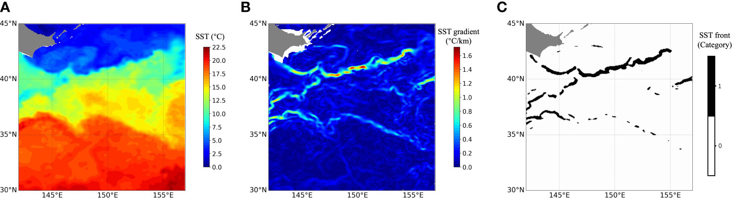
Figure 1 Data processing procedures in the OC region. (A) The SST data on 2 January, 2015, (B) front structures derived from physical quantities, and (C) fronts derived from threshold segmentation. The background is represented by category 0 and the SST front structure is represented by category 1.

$\begin{array}{ll}\begin{array}{cc}G\hfill & =\sqrt{G_x^2+G_y^2},\hfill \end{array}& (1)\end{array}$

$\begin{array}{ll}{G}_x(i,j)=\{\begin{array}{ll}(SST(i,j+1)-SST(i,j-1))/2,\hfill & j\ne 0\text{\hspace{0.17em}and\hspace{0.17em}}j\ne j_m-1,\hfill \\ SST(i,1)-SST(i,0),\hfill & j=0,\hfill \\ SST(i,j_m-1)-SST(i,j_m-2),\hfill & j=j_m-1,\hfill \end{array}& (2)\end{array}$

$\begin{array}{ll}{G}_y(i,j)=\{\begin{array}{ll}(SST(i+1,j)-SST(i-1,j))/2,\hfill & i\ne 0\text{\hspace{0.17em}and\hspace{0.17em}}i\ne i_m-1,\hfill \\ SST(1,j)-SST(0,j),\hfill & i=0,\hfill \\ SST(i_m-1,j)-SST(i_m-2,j),\hfill & i=i_m-1,\hfill \end{array}& (3)\end{array}$

where $G$ denotes the final gradients of the SST data in equation (1). In equation (2), $G_x$ denotes the zonal gradient of the SST data that is half of the difference between adjacent pixels in the zonal direction on the SST data, and $j_m$ is the last pixel value in the zonal direction. In equation (3), $i_m$ is the last pixel value in the meridional direction, and $G_y$ represents the meridional gradient of the SST data, which is half of the difference between adjacent pixels in the meridional direction on the SST data.

Figure 1B shows front structures obtained from the SST data using physical quantities to derive gradients. The nearshore front structures are excluded because the nearshore environment interferes with SST, resulting in data inaccuracies in experiments. The magnitude of the values of the front structures reflects their strength, which is significantly larger than that of the surrounding hydrographic elements. The final fronts can be obtained by setting the threshold $\theta$, where $0\le \theta \le 1.8$°C/km. This is due to the fact that the minimum gradient value is 0°C/km and the mean value of the maximum value of SST fronts for each day of the 10-year period in the OC region is 1.8°C/km. When using SST gradient data to obtain SST fronts, the size of the $\theta$ value needs to be selected based on experience and practical application scenarios. Figure 1C displays the SST fronts when the threshold $\theta =0.5$°C/km is used to segment front structures. Values exceeding 0.5°C/km are detected as SST fronts and assigned a value of 1, while values lower than 0.5°C/km are detected as non-SST fronts and assigned a value of 0.

In addition, the sea surface salinity (SSS) data are applied to verify the reliability and generalizability of the proposed MCSTNet. Similar to the SST data, the 8-year SSS data are used as a training set, from 1 January, 2006, to 31 December, 2013, and the 2-year SSS data are employed as a testing set, from 1 January, 2014, to 31 December, 2015. The daily SSS data, with a spatial resolution of 0.08° × 0.08°, from ERA5 reanalyses are generated by the Operational Mercator global ocean reanalysis system. Similarly, the target front structures are obtained using physical quantities to derive gradients of SSS. Hereafter, we substitute front for front structure in subsequent text.

2.2 The MCSTNet framework

The overall framework of MCSTNet is displayed in Figure 2, which is made up of three parts: the encoder-decoder structure, the time transfer module, and the memory-contextual module. The encoder-decoder structure is the backbone structure except for the time transfer module and memory-contextual module, which comprises a data encoder, a feature decoder, as well as a multi-task generation module. The encoder-decoder structure is used to extract the rich spatial features of input sequences and generate high-quality predicted spatial information. The time transfer module is applied to transfer temporal information and fuse low-level, fine-grained temporal information with high-level semantic information to improve medium- and long-term prediction precision. The memory-contextual module is employed to fuse low-level spatiotemporal information with high-level semantic information to enhance short-term prediction precision. Thus, MCSTNet is better at transferring spatiotemporal information for sequence prediction. As shown in Figure 2, the MCSTNet framework receives the previous SST sequences and predicts the future SST sequences and fronts.

FIGURE 2

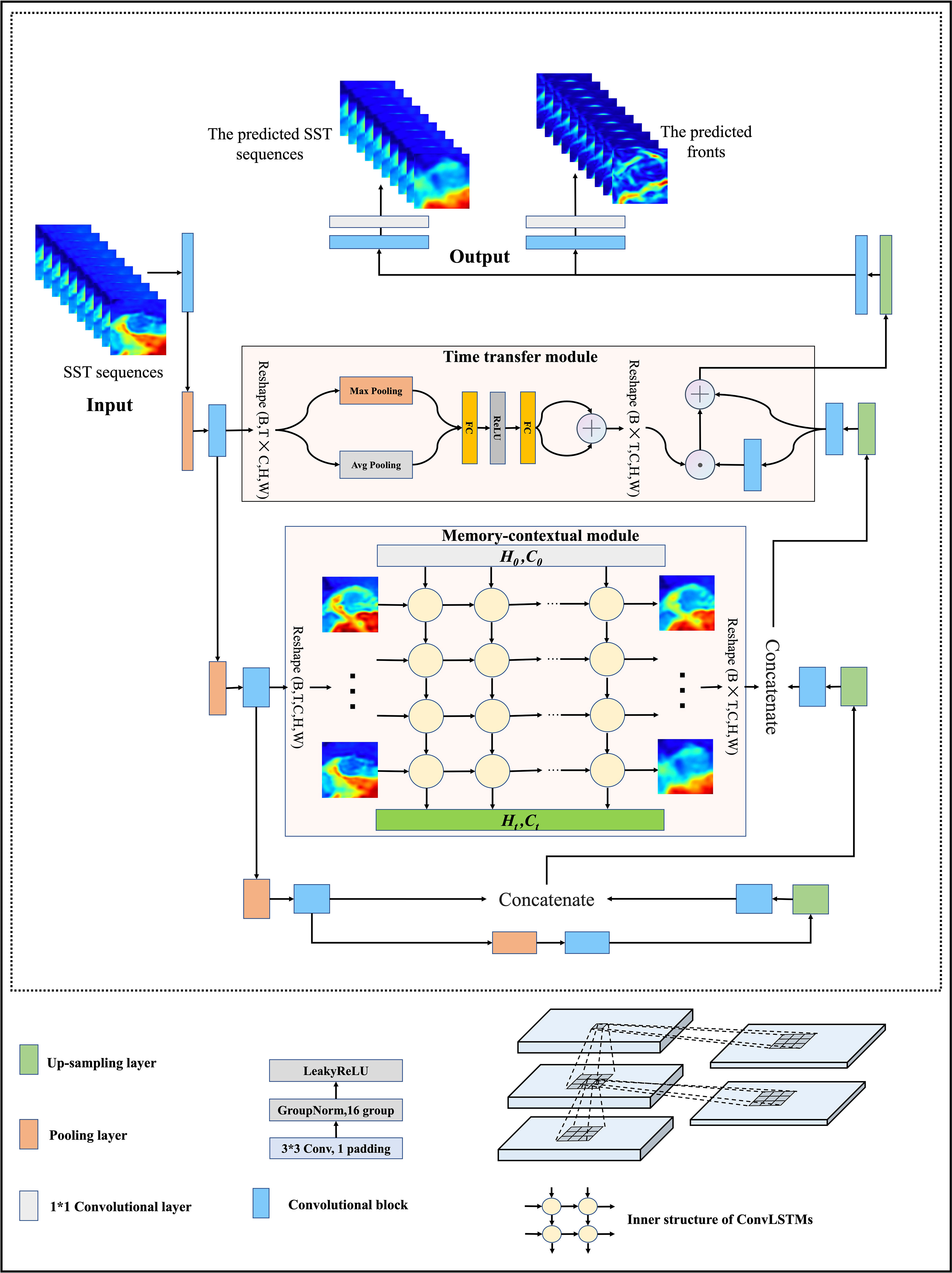
Figure 2 The MCSTNet framework. It includes three parts: the encoder-decoder structure, the time transfer module, and the memory-contextual module. MCSTNet receives SST sequences and then outputs the predicted SST sequences along with SST fronts.

2.2.1 The encoder-decoder structure

The encoder-decoder structure is made up of a data encoder, a feature decoder, and a multi-task generation module.

2.2.1.1 The data encoder

The convolutional block makes use of a 2D convolution that can only receive data in four dimensions, but the input data for the sequence prediction task has five dimensions ([batch, sequence length, number of input image channels, input image height, input image width]). Therefore, it is necessary to combine the batch and sequence length of the input data into one dimension, becoming four dimensions ([batch × sequence length, number of input image channels, input image height, input image width]). The first dimension is [batch x sequence length], treating all sequences as independent images. The transformed four-dimension data are fed into the data encoder, which includes four convolutional blocks and four max-pooling operations. The convolutional block consists of a 2D convolution with a convolution kernel of 3 × 3, a GroupNorm with a group size of 2, and a LeakyRelu. To ensure that the size of input and output data is the same, the 2D convolution uses the zero padding technique. The max-pooling operation, with a step size of 2, is employed between convolutional blocks to halve the size of feature maps.

2.2.1.2 The feature decoder

After the data encoder, the feature decoder is employed to decode the obtained high-level spatial sequence information. The feature decoder is made up of four convolutional blocks and four up-sampling layers with a factor of 2, which doubles the size of feature maps. The contextual feature maps obtained using the feature decoder are short on rich semantic information, while the semantic feature maps obtained using the data encoder are short on rich contextual information. The multi-scale feature maps from the data encoder and the feature decoder are connected using the memory-contextual module and the time transfer module to get the most out of the low-level contextual features and high-level semantic features of the input data, improving the quality of the predicted images.

2.2.1.3 The multi-task generation module

The multi-task generation module contains two sub-networks, each of which is made up of a convolutional block and a 2D convolution with a convolution kernel of 1 × 1. Two sub-networks receive the feature maps obtained by the feature decoder to generate the predicted SST and fronts, respectively.

2.2.2 The time transfer module

The time transfer module further extracts the temporal information from the shallow data encoder and transfers it to the deep feature decoder, enabling the transfer of the temporal information. To re-establish the temporal relationship between the image sequences, the features output from the shallow data encoder are dimensionally transformed from [batch × sequence length, number of input image channels, input image height, input image width] to [batch, sequence length × number of input image channels, input image height, input image width], to fuse the temporal and channel dimensions. Global self-adaptive max-pooling and global self-adaptive average pooling are performed in the channel dimension, respectively. The pooled features obtained are input to a two-layer, fully connected network with shared weights for non-linear transformation. The obtained features are added to the deep feature encoder output to obtain temporal feature information. After learning temporal feature information, the data needs to be transformed back to the shape it had before being input into the time transfer module to fuse the temporal information with the spatiotemporal features output by the deep feature decoder. The obtained features are dimensionally transformed, expanding the dimension to [batch, sequence length × number of input image channels, input image height, input image width], and then reshaping it to [batch × sequence length, number of input image channels, input image height, input image width]. Finally, the obtained temporal features and the deep spatial semantic features are multiplied element by element and added to achieve the transfer and fusion of temporal information.

2.2.3 The memory-contextual module

The memory-contextual module consists of ConvLSTMs with three hidden layers. The memory-contextual module learns spatiotemporal sequence information in the feature space from the shallow data encoder and transfers the learned spatiotemporal sequence information to the deep feature decoder, which learns information about object position changes in the image sequence, i.e., learns spatiotemporal sequence information about sequence changes. Specifically, the four-dimensional features output by the shallow data encoder are reshaped into five-dimensional spatiotemporal sequence features, which are fed into the memory-contextual module to learn the spatiotemporal sequence information. The obtained five-dimensional spatiotemporal sequence features are reshaped into four-dimensional features, which are concatenated with the spatiotemporal features output by the deep feature decoder to obtain the combined spatiotemporal sequence features.

2.2.4 Loss function

In this study, predictions of future SST sequence and front variation trend based on previous SST data are multi-task predictions, requiring a different loss function for each sub-network to guide the training of MCSTNet. Essentially, the SST sequence and front prediction tasks are image generation issues, i.e., it is necessary to determine whether the generated image sequence is similar to the real image sequence. In general, image similarity is measured using MSE, and the loss function is written as

$\begin{array}{ll}\begin{array}{ll}{L}_{MSE}(I,\widehat{I})\hfill & =\frac{1}{M·N}\sum _{i=0}^{M-1}\sum _{j=0}^{N-1}{[I(i,j)-\widehat{I}(i,j)]}^2.\hfill \end{array}& (4)\end{array}$

In equation (4), $M$ denotes the number of rows of predicted image pixels; $N$ denotes the number of columns of predicted image pixels; $I$ denotes the target SST or front images; $\widehat{I}$ denotes the predicted SST or front images; and $i,j$ denotes the position of each pixel. The lower the MSE value is, the more similar the two images are. MSE measures whether the predicted and target images have the same meaning in terms of corresponding pixels. Meanwhile, the feature similarity between the predicted and target images should be measured. Specifically, the predicted and target images are input into the ResNet-50 feature extractor, which uses a pre-trained model from ImageNet and weights sourced from He et al. (2016), to extract features, respectively, and the features output of the last lth layer are obtained. Generally, contextual loss is employed to determine the difference between features by calculating the cosine similarity. Because contextual loss measures the overall feature similarity of images, it can promote the prediction of non-stationary information.

When the cosine distance is small, they can be considered similar, and conversely, they are considered dissimilar. Thus, the issue of determining whether two features are similar is transformed into the issue of minimizing the cosine similarity between feature maps of the predicted and target images. Contextual loss is written as:

$\begin{array}{ll}\begin{array}{l}{L}_{CX}(y_p,y_t,l)=1-cos({\text{Φ}}^l(y_p),{\text{Φ}}^l(y_t)),\hfill \end{array}& (5)\end{array}$

where $y_p$ represents the predicted SST or fronts, $y_t$ represents the target SST or fronts, $\text{Φ}$ represents a ResNet-50 pre-trained feature extractor, and $l$ represents the last lth layer of the ResNet-50 in equation (5).

Combining the advantages of MSE in tackling stationary information and the virtues of contextual loss in tackling non-stationary information, the overall loss function is jointly guided by two loss functions and is written as:

$\begin{array}{ll}\begin{array}{l}{L}_{Front}=L_{SST}=\lambda L_{CX}+(1-\lambda )L_{MSE}.\hfill \end{array}& (6)\end{array}$

In equation (6), $\lambda$ is an equilibrium factor to balance the two loss functions, which is usually determined based on experimentation and experience ($\lambda =0.2$ in our experiments). MCSTNet makes use of a multi-task training mode to predict SST sequence and front images, respectively. Although MCSTNet has two prediction sub-networks, i.e., the SST prediction sub-network and the front prediction sub-network, the predicted results only differ in data, so the loss functions of these two prediction sub-networks can be the same. The final loss function of MCSTNet is the sum of the loss functions of the SST prediction sub-network and the front prediction sub-network and is written as:

$\begin{array}{ll}\begin{array}{l}{L}_{MCSTNet}=L_{SST}+L_{Front}.\hfill \end{array}& (7)\end{array}$

3 Experiment

In the experiments, the excellent spatiotemporal sequence prediction capability of our proposed MCSTNet is reported and compared with SOTA sequence prediction models based on the SST data. The generalization of MCSTNet is verified based on the SSS data. Furthermore, the effectiveness of each module in MCSTNet is evaluated.

3.1 Experimental settings

In this section, we introduce the MCSTNet training process and experimental platform configuration.

3.1.1 The training process of MCSTNet

In this study, MCSTNet was used for the SST sequence and front prediction tasks that required learning the stationary and non-stationary information in SST sequences. Its training process was extremely challenging, and it might be difficult to fit the network during the training process. To facilitate network fitting, MCSTNet introduced a probability of using the target SST during the training process. Specifically, MCSTNet set a decreasing probability value with increasing iteration steps, which meant that the target sequences were used to substitute the predicted sequences with a certain probability when training the memory-contextual module.

The training process of MCSTNet is shown in Algorithm 1. During the training process, MCSTNet received the input SST sequences of length 10 with random sampling, the target SST sequences, and the probability of using the target SST. The input SST sequences and the target SST sequences were fed into the data encoder and feature encoder to extract features, respectively. When generating each predicted SST feature, based on the probability of using the target SST, the predicted SST sequence features are substituted for the target SST sequence features. This enables the memory-contextual module to learn the spatiotemporal feature information well, making the whole network stable during training. The initial value of the probability was approaching 1.0, which decreased with increasing iteration steps, eventually decreasing to zero. When the value of this probability was zero, the whole network was predicted using all the input SST sequences. During the test, the value of this probability was always set to zero.

3.1.2 Experimental platform configuration

The experimental platform configuration is as follows. The server operating system is Ubuntu 20.04.4 LTS, with 2 physical cores and 56 logical CPU cores, 128 GB of memory, and two NVIDIA 3090 Ti graphics cards. The software development environment relies on Linux, and the development language is Python 3.7.11. The DL framework used is Pytorch 1.12.0, which is widely used for DL. It is a flexible and efficient DL framework with an underlying C++ implementation. To make a fair comparison, we set the hyperparameters for MCSTNet and other comparative methods to be consistent. A detailed list of hyperparameters for MCSTNet and other comparative methods is presented in Table S2.

ALGORITHM 1 THE TRAINING PROCESS OF MSTNET.

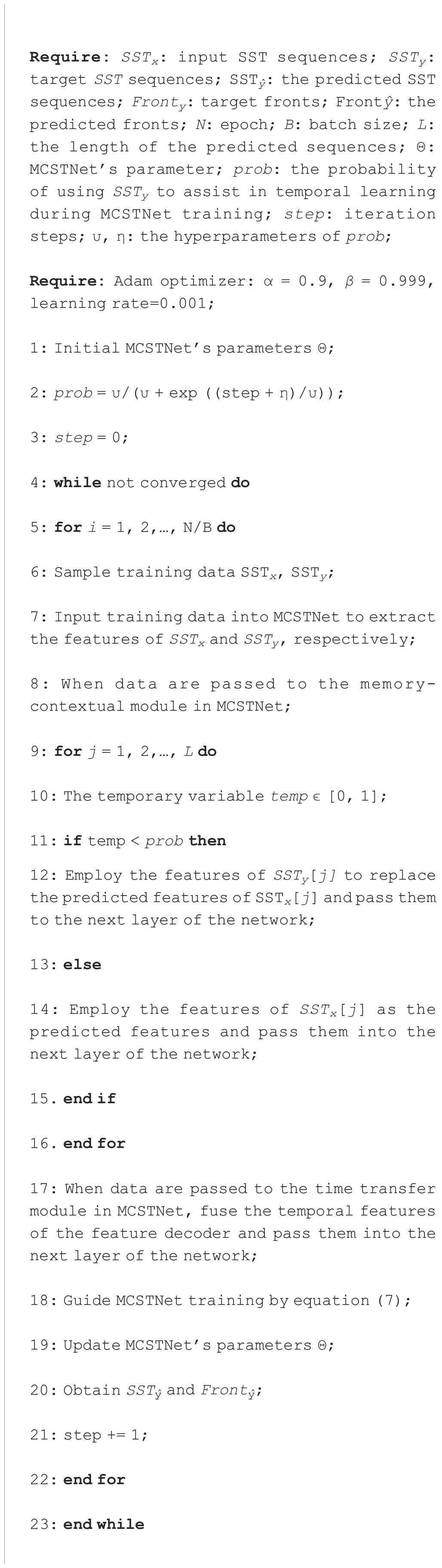
Algorithm 1 The training process of MSTNet..

3.2 Comparative approaches

In our experiments, the SOTA models incorporated physical constraints-based PhyDNet (Guen and Thome, 2020), RNNs-based ConvLSTM (Shi et al., 2015), PredRNN (Wang et al., 2017), PredRNNv2 (Wang et al., 2021), as well as MIM (Wang et al., 2019), and CNNs-based SimVP (Gao et al., 2022), which were used as comparative approaches to compare with our proposed MCSTNet.

PhyDNet introduces a recurrent physical cell to model physical dynamics for discretizing the restriction of the partial differential equation (PDE) and is a global sequence to sequence DL-based approach. It is the first study to achieve good predictive performance by combining physical constraints with DL.

ConvLSTM innovatively combines CNN and LSTM for predicting sequences of images, enabling the capture of both spatial and temporal sequences, and has been applied to a real-life radar echo dataset for precipitation nowcasting. Each layer of the CNN structure encodes spatial information, while the memory units encode temporal information independently.

PredRNN is proposed by Wang et al. (2017), a novel recurrent network in which two memory cells are used to extract the variance of spatiotemporal information, improving the predictive power of spatiotemporal sequences. Wang et al. (2021) propose an enhancement to the PredRNN structure, dubbed PredRNNv2, which is expanded to predict action-conditioned video. During the training period, reverse scheduled sampling is employed to learn the dependencies between jumpy frames by arbitrarily hiding the training data and changing with certain probabilities.

Memory in memory (MIM) is proposed by Wang et al. (2019), an upgraded form of LSTM in which two inbuilt long short-term memories substitute for the forget gate of LSTM. MIM, with its two cascaded and self-renewed memory structures, makes use of differential information between neighboring recurrent states to model for nearly stationary and non-stationary spatiotemporal features. Higher-order non-stationarity can be dealt with by stacking MIM structures.

SimVP is proposed by Gao et al. (2022), which only uses CNN structure and simple MSE loss for video prediction. SimVP learns the spatial information of the images using a normal CNN structure and learns the temporal information in the video sequences using an inception structure-based CNN, enabling the prediction of spatiotemporal information in video sequences.

3.3 Experimental results

In this section, to test the capability of MCSTNet to predict sequences and transfer spatiotemporal information, we conducted preliminary experiments on the Moving MNIST dataset (see Figures S1, S2; Table S1). Moreover, we conducted comparison experiments to verify the excellent spatiotemporal sequence prediction capability of MCSTNet on the SST data. The SSS data were used to verify the r eliability and generalizability of MCSTNet, and ablation studies were conducted to demonstrate the effectiveness of each module in MCSTNet.

3.3.1 SST sequence and front predictions based on the SST data

To demonstrate the advantages of the MCSTNet framework in predicting SST sequences and fronts, we compared MCSTNet to comparative approaches for both quantitative and qualitative assessments based on the SST data.

3.3.1.1 Qualitative assessment

Figure 3 displays the predicted results of the future 10-day SST sequences and front images using MCSTNet based on the previous 10-day satellite SST sequences, and only the images for the even-numbered days are plotted. The time horizon of SST images and front images is 20 days, from 6 March, to 25 March, 2015, with a latitude range of 39.3°N–42.5°N and a longitude range of 145.2°E–148.4°E. The predicted front images corresponding to SST sequences in the future 10 days were obtained by MCSTNet through learning the SST variation laws in the previous 10 days. At the beginning of the prediction (T = 11 and 13), the predicted SST sequences and fronts are similar to the target SST and fronts. As the prediction time increases, although the predicted SST sequences and fronts deviate somewhat from the target SST and fronts, the overall variation trend of the SST sequences and fronts is consistent with the target. This is due to the large time span of the SST data, which results in the large variability of the SST data. The variation trend of SST sequences and fronts predicted by MCSTNet is reasonable and authentic. It reveals that MCSTNet is effective for SST sequence prediction and front variation trend prediction.

FIGURE 3

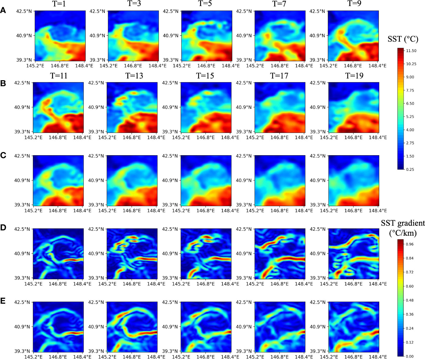
Figure 3 Satellite and predicted SST sequences, physics-based and predicted fronts at five successive sequences with 1-day intervals. The previous 10-day satellite SST sequences are input into MCSTNet to predict future 10-day SST sequences and fronts. (A) Input SST sequences on 6, 8, 10, 12, and 14 March, 2015. (B) Target SST, (C) the predicted SST, (D) target frons, and (E) the predicted fronts, on 16, 18, 20, 22, and 24 March, 2015.

Figure 4 displays the predicted results of the future 10-day SST sequences using MCSTNet and comparative approaches based on the previous 10-day satellite SST sequences, and only the images for the even-numbered days are plotted. From the thirdline, each line displays the future 10-day SST sequences predicted by MCSTNet, SimVP, PhyDNet, PredRNNv2, MIM, PredRNN, and ConvLSTM, based on SST variation laws, respectively. Because of the normalization technique used during the training on the SST data, some of the training data was close to zero, making PredRNNv2 and MIM difficult to train and producing poorer visualization results. The visual results show that CNNs-based models predict significantly better than those only relying on RNNs, indicating that CNNs are helpful for image detail processing. Compared to SimVP, which uses only the CNN structure, MCSTNet predicts SST sequences better. In particular, medium-term SST sequences predicted by MCSTNet are more accurate. Compared to Figure 4E, MCSTNet predicts significantly better. This is because it is difficult to use a certain physical model to constrain non-stationary SST data, resulting in PhyDNet predicting SST worse. RNNs-based models, including PredRNN, PredRNNv2, MIM, and ConvLSTM, are good at predicting data with a stable and constant shape in the image but perform poorly in predicting image details on non-stationary SST data, leading to poor quality of the predicted images. MCSTNet combines the detailed learning ability of the CNN module with the variation pattern learning ability of the RNN module, which takes into account the non-stationary information and detailed features of SST sequences, and obtains more authentic and reasonable predicted results than comparative approaches. It demonstrates that MCSTNet is the most appropriate approach for the SST sequence prediction task.

FIGURE 4

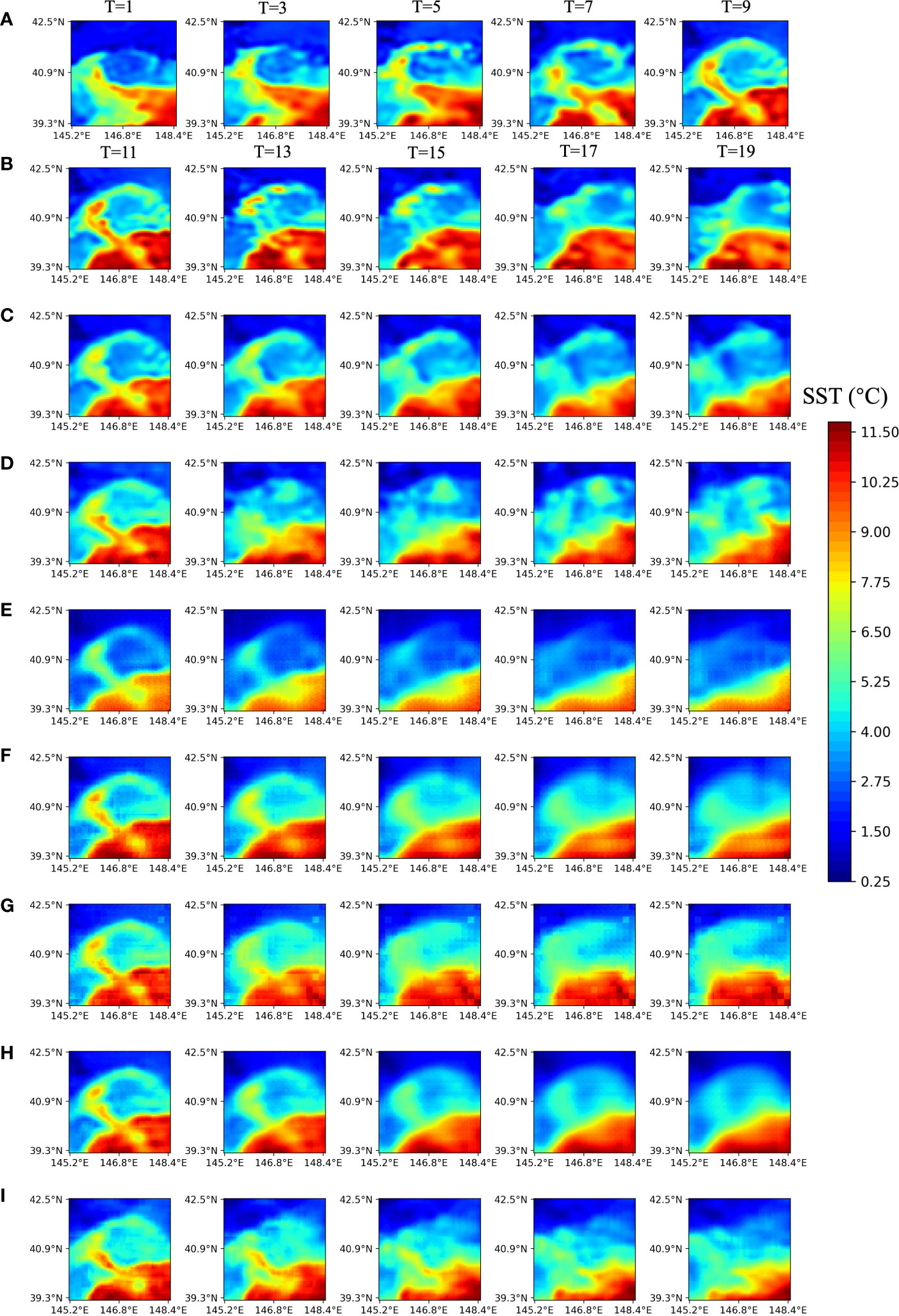
Figure 4 Satellite and predicted SST sequences at five successive sequences with 1-day intervals by MCSTNet and the compared approaches. The previous 10-day satellite SST sequences are employed to predict future 10-day SST sequences. (A) Input SST sequences on 6, 8, 10, 12, and 14 March, 2015. (B) Target SST sequences, and the predicted SST sequences by (C) MCSTNet, (D) SimVP, (E) PhyDNet, (F) PredRNNv2, (G) MIM, (H) PredRNN, as well as (I) ConvLSTM on 16, 18, 20, 22, and 24 March, 2015.

Figure 5 displays the 1-day results as well as the SST and front error images between target and prediction. The target SST and front denote the future 1-day SST and physical-based fronts, respectively, and are on 27 October, 2014, and 13 February, 2015. MCSTNet received the previous 10-day satellite SST sequences to predict the future 10-day SST sequences and front images. The SST and fronts error images were obtained by taking the absolute value of the differences between the target and predicted SST and the target and predicted fronts. For each line in the error images, the maximum and average errors are: the first line with a maximum error of 1.572°C and an average error of 0.350°C; the second line with a maximum error of 0.282°C/km and an average error of 0.039°C/km; the third line with a maximum error of 1.157°C and an average error of 0.197°C; and the fourth line with a maximum error of 0.302°C/km and an average error of 0.040°C/km. From the statistical data and visual results, despite the relatively high maximum error of the predicted data, the relatively small average error indicates that the overall prediction performance of MCSTNet is relatively stable. It indicates that MCSTNet is appropriate for SST sequence and front prediction tasks.

FIGURE 5

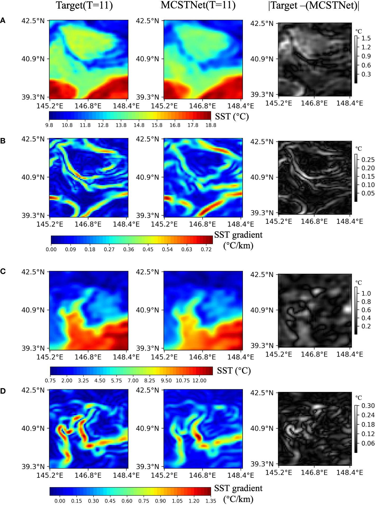
Figure 5 Satellite and predicted SST sequences, physics-based and predicted fronts, and the error between them. The previous 10-day satellite SST sequences are employed to predict future 10-day SST sequences and fronts, but only one day is plotted. From left to right, each column represents target SST sequences and fronts, the predicted SST sequences and fronts by MCSTNet, and the SST and front error between target and predicted by MCSTNet (absolute value). There are two examples of SST and front predictions: (A, B) show images from 26 October, 2014 to 27 October, 2014, while (C, D) show images from 12 February, 2015 to 13 February, 2015.

We predicted not only short- and medium-term SST sequences and fronts but also long-term SST sequences and fronts. Figure 6 displays the predicted results of the future 30-day SST sequences using MCSTNet and comparative approaches based on the previous 30-day satellite SST sequences, and only the images at five successive sequences with 5-day intervals are plotted. From the third line, each line displays the future 30-day SST sequences predicted by MCSTNet, SimVP, PredRNNv2, MIM, PredRNN, and ConvLSTM, based on SST variation laws, respectively. All models show that the performance of the short-term prediction is better than that of the medium-term, and that of the medium-term is better than that of the long-term. As the predicted time increases, the authenticity and precision of the predicted SST sequences by all models decrease. However, our proposed MCSTNet predicts higher-quality SST sequences than the comparison method, with clearer images, richer detail, and more accurate SST variation patterns. This demonstrates that MCSTNet is beneficial for learning fine-grained, long-term spatiotemporal information about SST sequence variation laws.

FIGURE 6

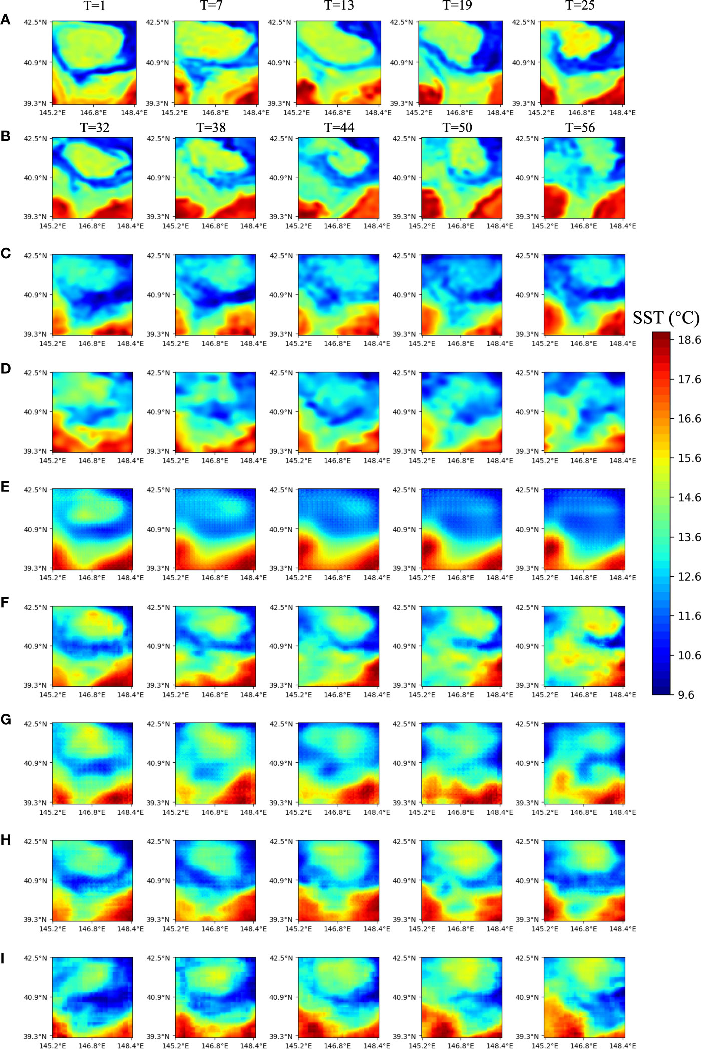
Figure 6 Satellite and predicted SST sequences at five successive sequences with 1-day intervals by MCSTNet and the compared approaches. The previous 30-day satellite SST sequences are used to predict future 30-day SST sequences. (A) Input SST sequences on 16, 22, 28 October, and 3, 9 November, 2014. (B) Target SST sequences, and the predicted SST sequences by (C) MCSTNet, (D) SimVP, (E) PhyDNet, (F) PredRNNv2, (G) MIM, (H) PredRNN, as well as (I) ConvLSTM on 15, 21, 27 November, and 3, 9 December, 2014.

3.3.1.2 Quantitative assessment

To quantificationally evaluate the authenticity and quality of the predicted SST and front images by MCSTNet and comparative approaches, the MSE (Prasad and Rao, 1990), mean absolute error (MAE) (Willmott and Matsuura, 2005), structural similarity (SSIM) (Wang et al., 2004) and peak signal-to-noise ratio (PSNR) (Huynh-Thu and Ghanbari, 2008) were selected as evaluation indices. Specifically, the deviation between the predicted and target images was measured by MSE and MAE. MSE evaluates the ability of models to measure abnormal data, while MAE evaluates the ability of models to measure most data. MAE is calculated as:

$\begin{array}{ll}\begin{array}{ll}MAE(I,\widehat{I})\hfill & =\frac{1}{M·N}\sum _{i=0}^{M-1}\sum _{j=0}^{N-1}|I(i,j)-\widehat{I}(i,j)|,\hfill \end{array}& (8)\end{array}$

where $I$ is the target images, $\widehat{I}$ is the predicted images, $M$ is the number of rows of images, and $N$ is the number of columns of images in equation (8).

The structural similarity between the target and predicted images was measured by SSIM, which measured image similarity in terms of luminance, contrast, and structure, respectively. Specifically, the comparison of luminance compares the local variations in brightness or intensity of pixels between the two images by calculating the standard deviation of the pixel intensities within a small region of the image. The structure comparison compares the spatial patterns of the pixels in each image by calculating the correlation between different regions of the images. SSIM is written as:

$\begin{array}{ll}\begin{array}{ll}SSIM(I,\widehat{I})\hfill & =[l(I,\widehat{I}){]}^{\alpha }[c(I,\widehat{I}){]}^{\beta }{[s(I,\widehat{I})]}^{\gamma }\hfill \\ \hfill & =\frac{(2{\mu }_I{\mu }_{\widehat{I}}+c_1)({\sigma }_{I\widehat{I}}+c_2)}{({\mu }_I^2+{\mu }_{\widehat{I}}^2+c_1)({\sigma }_I^2+{\sigma }_{\widehat{I}}^2+c_2)},\hfill \end{array}& (9)\end{array}$

where $l(I,\widehat{I})$ represents the luminance comparison between the target and predicted images; $c(I,\widehat{I})$ represents the contrast comparison between the target and predicted images; $s(I,\widehat{I})$ represents the structure comparison between the target and predicted images; ${\mu }_I$ and ${\mu }_{\widehat{I}}$ are the mean values of $I$, $\widehat{I}$, respectively; ${\sigma }_I$, ${\sigma }_{\widehat{I}}$, and ${\sigma }_{I\widehat{I}}$ denote the covariances of $I$, $\widehat{I}$, as well as $I\widehat{I}$, respectively; $\alpha$, $\beta$, and $\gamma$ are hyper-parameters; and constants $c_1$ as well as $c_2$ are used to avoid zero denominator issue in equation (9).

The quality of the maximum possible value of the target and predicted images was assessed by PSNR. It is calculated as $10·{\log }_{10}\frac{MA{X}_I^2}{MSE}$, where $MA{X}_I^2$ is the maximum pixel value of images. Higher image quality is represented by smaller MSE and MAE values, as well as bigger SSIM and PSNR values.

Tables 1, 2 show the values of MSE, MAE, PSNR, and SSIM obtained by MCSTNet and the compared approaches concerning 10- and 30-day SST sequence prediction on the SST data, respectively. Compared to the other models, our proposed MCSTNet obtains the best values on all evaluation indices for both the 10- and 30-day prediction results. As the predicted time increases, the authenticity and accuracy of the predicted SST sequences decrease for all models. The values for both MSE and MAE are meaningfully lower than those of comparative approaches, and those for PSNR and SSIM are slightly higher than those of comparative approaches. It reveals that MCSTNet is superior to comparative approaches, and the predicted SST sequences by MCSTNet are the most authentic and reasonable than comparative approaches.

TABLE 1

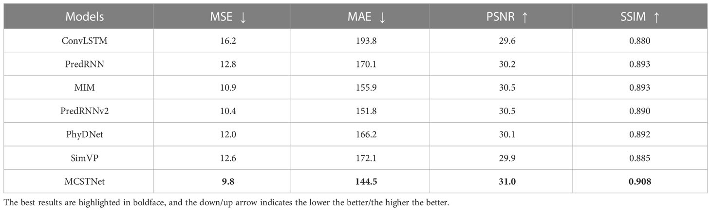
Table 1 Comparison of the results of 10-day SST spatiotemporal sequence prediction between MCSTNet and other approaches in terms of MSE, MAE, PSNR and SSIM on the SST data.

TABLE 2

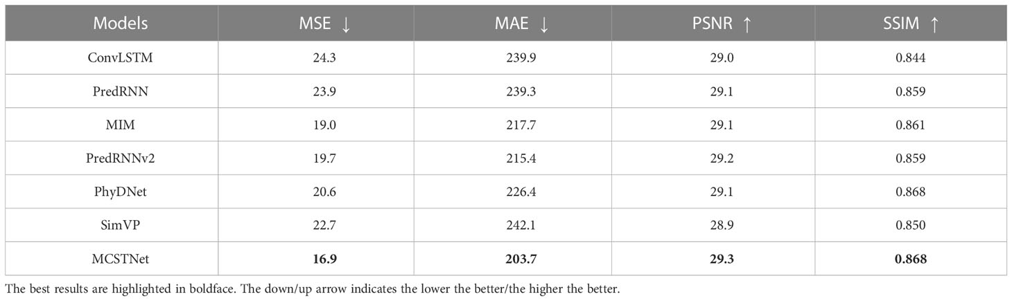
Table 2 Comparison of the results of 30-day SST spatiotemporal sequence prediction between MCSTNet and other methods in terms of MSE, MAE, PSNR and SSIM on the SST data.

3.3.2 Verification of the generalization of MCSTNet based on the SSS data

To verify the generalization of our proposed MCSTNet, in addition to the SST data, we also made use of MCSTNet to predict SSS sequences and fronts on the SSS data.

Figure 7 depicts the predicted future 10-day SSS sequences and front images with even-numbered days by MCSTNet, based on previous 10-day satellite SSS sequences. The SSS sequences and front images have a temporal window of 20 days, from 6 March, to 25 March, 2015, with latitudes ranging from 35.6°N to 40.8°N and longitudes ranging from 142.0°E to 147.2°E. The fronts were predicted by MCSTNet based on learning the SSS variation laws in the previous 10 days. Compared to the target, the predicted SSS sequences and fronts using MCSTNet are authentic and reasonable, which demonstrates that MCSTNet is effective and appropriate for SSS sequence prediction and front variation tendency prediction tasks.

FIGURE 7

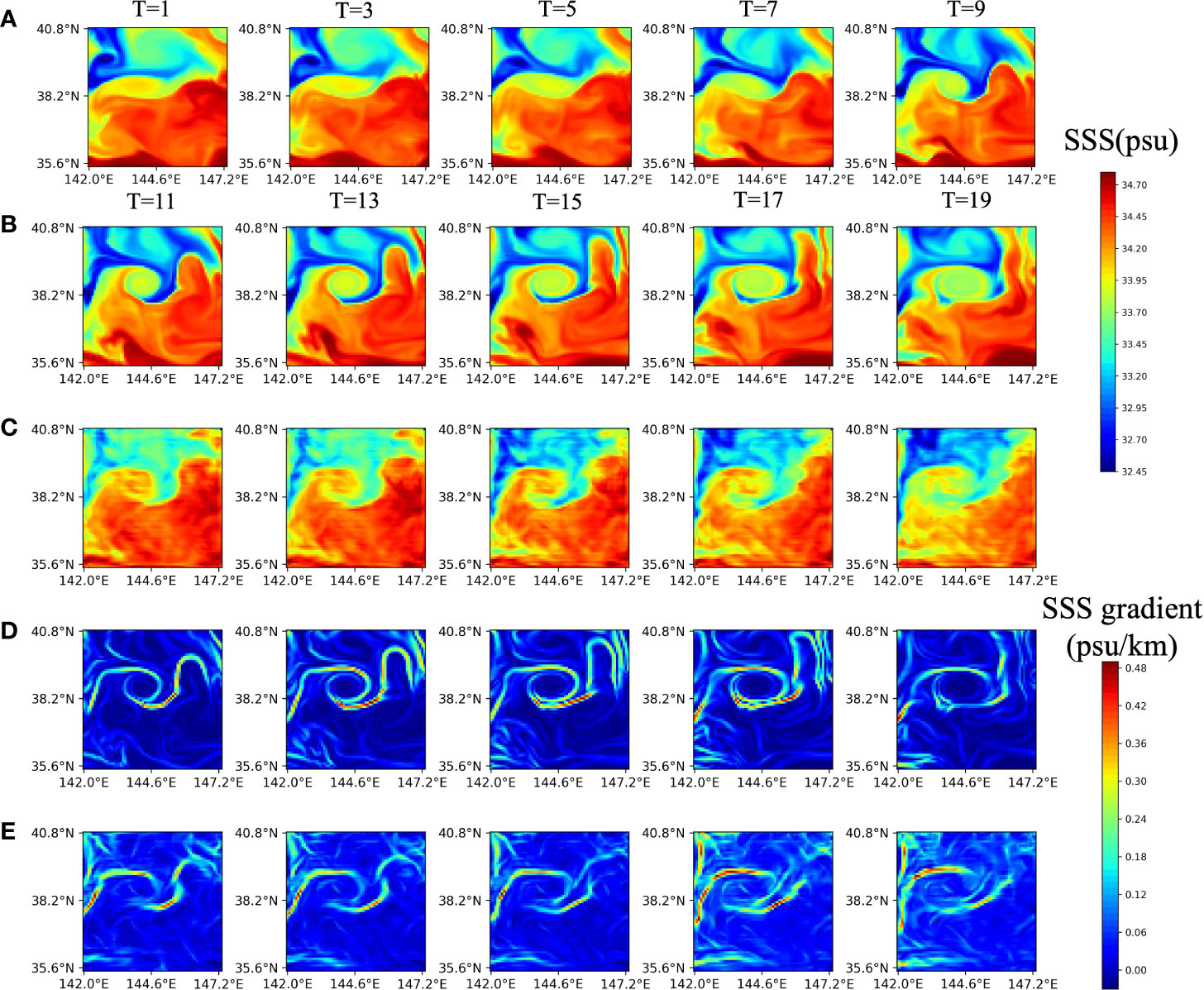
Figure 7 Satellite and predicted SSS sequences, physics-based and predicted fronts at five successive sequences with 1-day intervals. The previous 10-day satellite SSS sequences are employed to predict future 10-day SSS sequences and fronts. (A) Input SSS sequences on 6, 8, 10, 12, and 14 March, 2015. (B) Target SSS, (C) the predicted SSS, (D) target fronts, and (E) the predicted fronts on 16, 18, 20, 22, and 24 March, 2015.

Figure 8 shows the 1-day images as well as the SSS and front error images. MCSTNet predicted the future 10-day SSS and front images based on the previous 10-day SSS data. We calculated the absolute value of the SSS and front errors as the difference between the target and the predicted SSS and front using MCSTNet. SSS and front errors are mostly found in the locations of extreme SSS as well as the front and are numerically small. The results demonstrate that MCSTNet is accurate for SSS sequence and front prediction tasks.

FIGURE 8

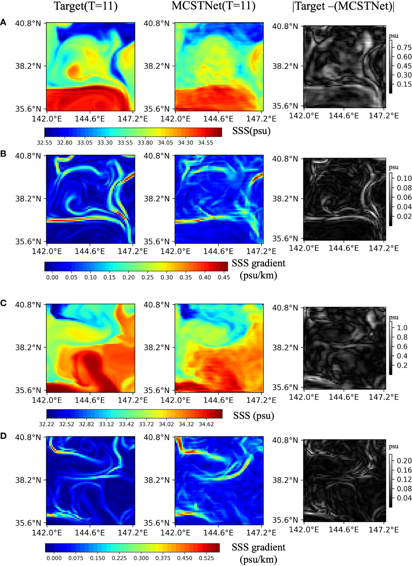
Figure 8 Satellite and predicted SSS sequences, physics-based and predicted fronts, and the error between them. The previous 10-day satellite SSS sequences are used to predict future 10-day SSS sequences and fronts, but only one day is plotted. From left to right, each column represents target SSS sequences and fronts, the predicted SSS sequences and fronts by MCSTNet, and the SSS and front error between target and predicted by MCSTNet (absolute value). There are two examples of SSS and front predictions: (A, B) show images from 26 October, 2014 to 27 October, 2014, while (C, D) show images from 12 February, 2015 to 13 February, 2015.

The values of MSE, MAE, PSNR, and SSIM of SSS sequence prediction images obtained by MCSTNet and comparative approaches are shown in Table 3. The best values on all evaluation indices for the 10-day SSS sequence prediction images are obtained by MCSTNet compared to the other models. MSE and MAE values are significantly lower than those of comparative approaches, and PSNR and SSIM values are somewhat higher. This demonstrates that MCSTNet outperforms comparative approaches, and using MCSTNet to predict SSS sequences is reasonable.

TABLE 3

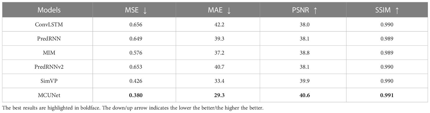
Table 3 Comparison of the results of 10-day SSS sequence prediction images between MCSTNet and other approaches in terms of MSE, MAE, PSNR and SSIM on the SSS data.

3.3.3 Ablation studies

To demonstrate the effectiveness of the encoder-decoder structure, the memory-contextual module (MCM), and the time transfer module (TTM) in MCSTNet, ablation studies were done.

Figure 9 shows the predicted future 10-day front images with odd-numbered days using each module in MCSTNet based on the previous 10-day satellite SST sequences. From the third line, each line displays the future 10-day front predicted using MCSTNet, MCSTNet without TTM, MCSTNet without MCM, and the encoder-decoder structure. The results demonstrate that the model using only the encoder-decoder structure is basically unable to predict the trend of fronts. The performance of the MCSTNet without MCM model, i.e., combining TTM with the encoder-decoder structure, outperforms the encoder-decoder structure. This is because TTM transfers temporal information and fuses low-level, fine-grained temporal information with high-level semantic information to improve medium- and long-term prediction precision. MCSTNet without TTM, i.e., combining MCM with the encoder-decoder structure, achieves good predictive results. This is because MCM can fuse low-level spatiotemporal information with high-level semantic information, and the quality of predicted fronts decreases with increasing prediction time, while the encoder-decoder structure extracts fine-grained features to precisely complement this shortcoming. In contrast to the aforementioned models, the MCSTNet model, which uses all modules, including the MCM, TTM, and encoder-decoder structure, not only predicts the front variation trend but also generates high-quality fronts. This is important for the prediction of fronts and illustrates that our proposed encoder-decoder structure, MCM, and TTM, help with the front prediction task.

FIGURE 9

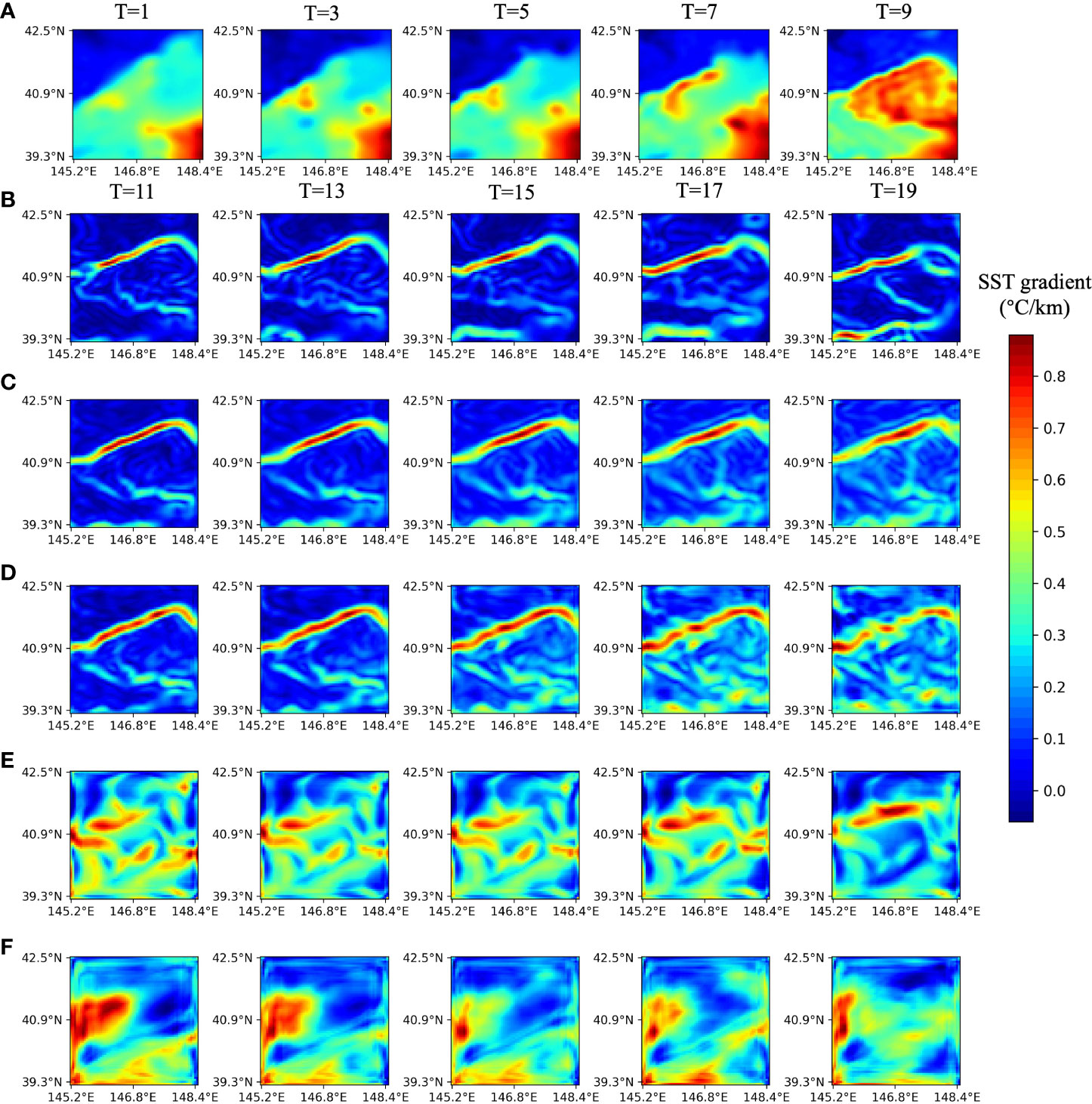
Figure 9 Visualization of the benefit of each module in MCSTNet on the SST data. The previous 10-day satellite SST sequences are used to predict future 10-day fronts. (A) Input SST sequences on 17, 19, 21, 23, and 25 February, 2014. (B) Target fronts, and the predicted fronts by (C) MCSTNet, (D) MCSTNet without TTM, (E) MCSTNet without MCM, as well as (F) encoder-decoder structure on 27 February, and 1, 3, 5, 7 March, 2014.

To further investigate the effectiveness of each module in MCSTNet for the front prediction task, we calculated the precision of front prediction, which represents the probability of a correct front prediction and whose formula is written as:

$\begin{array}{ll}\begin{array}{l}Precision(I_{mask},{\widehat{I}}_{mask})=\frac{{\sum }_{i=0}^{M-1}{\sum }_{j=0}^{N-1}[I_{mask}(i,j)*{\widehat{I}}_{mask}(i,j)]+ϵ}{{\sum }_{i=0}^{M-1}{\sum }_{j=0}^{N-1}[{\widehat{I}}_{mask}(i,j)]+ϵ}.\hfill \end{array}& (10)\end{array}$

In equation (10), $I_{mask}$ and ${\widehat{I}}_{mask}$ represent mask maps of target and predicted front images, respectively, obtained by setting a threshold value to fronts. In the mask maps, the region with fronts was set to 1, and the region without fronts was set to 0. $M$ and $N$ denote the total number of pixels in the meridional and zonal directions of images, respectively; $i$ and $j$ are the pixel positions; and $ϵ=0.00001$ is the parameter to prevent the division-by-zero issue.The range of the precision value is 0 to 1, and the larger the better.

The predicted front precision variation with the threshold taken by fronts and the predicted number of days, using each module in MCSTNet, is shown in Figure 10. Comparing Figures 10A, B, there is an improvement in the predicted front precision using TTM over the encoder-decoder structure. Especially for the medium-term front prediction, the precision improvement is more obvious, indicating that TTM learns information about the temporal variation information in the sequence. By comparing Figures 10A, C, the use of MCM can substantially improve the ability of sequence prediction. In particular, the improvement is more pronounced for the short-term front prediction but not for the medium-term front prediction. When comparing Figures 10A-D, the values of the predicted front precision by MCSTNet are significantly higher than those of using only a single module. This is because the MCSTNet model combines the medium- and long-term sequence prediction benefits of TTM with the short-term, high-quality prediction capability of MCM, making improvements for both short-, medium-, and long-term prediction. The precision of the front prediction decreases as the predicted time increases for all models, which is consistent with the characteristics of the prediction task.

FIGURE 10

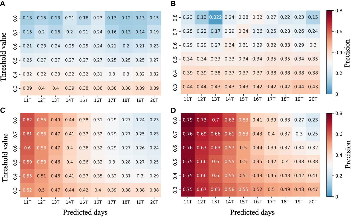
Figure 10 The precision of fronts predicted by MCSTNet and its subnetwork. Precision of front for (A) the encoder-decoder structure, (B) MCSTNet without MCM, (C) MCSTNet without TTM, and (D) MCSTNet.

The fronts predicted by MCM and TTM were evaluated objectively using the MSE, MAE, PSNR, and SSIM evaluation indices, as shown in Table 4. Both MCM and TTM have an enhancing effect on the prediction ability of fronts, and the enhancing effect of MCM is greater than that of TTM. This is because TTM is only a temporal feature information transfer model, while MCM transfers both temporal and spatial information. The simultaneous use of both modules obtains the best values in terms of all evaluation indices.

TABLE 4

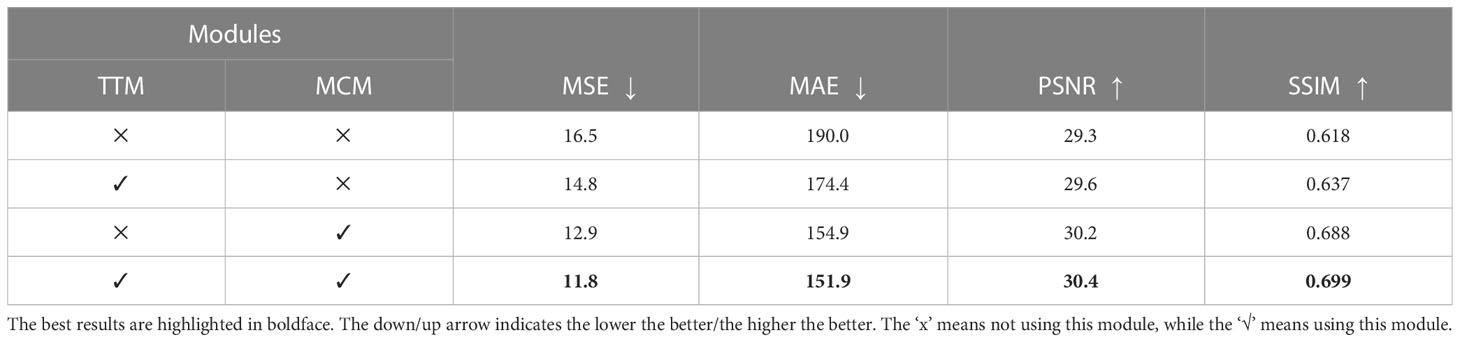
Table 4 Quantitative comparison of the future 10-day fronts predicted using the modules, i.e., MCM and TTM in MCSTNet, concerning MSE, MAE, PSNR, and SSIM on the SST data.

4 Conclusion and future work

Inspired by the virtues of the U-Net and ConvLSTM architectures, this paper proposes a continuous spatiotemporal prediction model, called MCSTNet, for predicting future spatiotemporal variation sequences of SST and fronts based on continuous mean daily SST data. The methodology of MCSTNet contains three components: the encoder-decoder structure, the time transfer module, and the memory-contextual module. The encoder-decoder structure consists of the data encoder, feature decoder, and multi-task generation module. The rich contextual and semantic information in SST sequences and frontal structures from the SST data is extracted by the encoder-decoder structure. The temporal information is transferred, and low-level fine-grained temporal information is fused with high-level semantic information to enhance the medium- and long-term prediction precision of SST sequences and fronts by the time transfer module. The low-level spatiotemporal information is fused with high-level semantic information to improve the short-term prediction precision of SST sequences and fronts using the memory-contextual module. Combining the virtues of MSE loss and contextual loss collectively guides MCSTNet for stability training during the training phase. Qualitative and quantitative experimental results demonstrate that the performance of MCSTNet is superior to the SOTA models on the SST data, which include physical constraints-based PhyDNet, RNNs-based ConvLSTM, PredRNN, PredRNNv2, as well as MIM, and CNNs-based SimVP. This is because MCSTNet combines the detail learning ability of the CNN module with the variation pattern learning ability of the RNN module, which takes into account the variation pattern and detail features of SST sequences. The above-mentioned method, such as PhyDNet, still has room for improvement in long-term spatiotemporal prediction. It is recommended to add skip connections in the shallow encoder module of PhyDNet so that fine-grained spatiotemporal information can be transferred to the deep decoder module, similar to the time transfer module proposed in this study. The time transfer module can be improved to transfer fine-grained spatiotemporal information, thus improving the long-term prediction ability of PhyDNet. Moreover, the SSS data are applied to verify the performance and generalization ability of MCSTNet, and the results show that the predicted SSS sequences and fronts by MCSTNet are authentic and reasonable. Ablation studies demonstrate the effectiveness of each module in MCSTNet, including the excellent feature extraction capability of the encoder-decoder structure, the short-term prediction capability of the memory-contextual module, and the medium- and long-term prediction benefits of the time transfer module.

Due to the limitations of computer computing power, fronts in the Oyashio current region have been studied. DL methods have the ability of transfer learning, where the knowledge learnt from one dataset can be applied to another dataset, making them ideal for training on SST data in one region and then being applied to other regions. The model’s prediction effectiveness can be enhanced by including data from the target area during training. In the future, we will expand our work to a larger scale or even a global scale to predict global SST sequences and fronts. Furthermore, we intend to add self-attention modules (Vaswani et al., 2017) to further improve the performance of MCSTNet. The DL methodology holds the promise of guiding the exploration of next-prediction “smart” SST sequences and fronts by harnessing our observational and theoretical knowledge to promote the development of this field.

Data availability statement

The original contributions presented in the study are included in the article/Supplementary Material. Further inquiries can be directed to the corresponding authors.

Author contributions

YM contributed to conceptualization, methodology, writing-original draft preparation and software. WL contributed to investigation, software and verification. GC contributed to editing and funding acquisition. GZ contributed to supervision, writing-reviewing and funding acquisition. FT contributed to data preparation, visualization and project administration. All authors contributed to the article and approved the submitted version.

Funding

This work was partially supported by the International Research Center of Big Data for Sustainable Development Goals under Grant No. CBAS2022GSP01, the National Key Research and Development Program of China under Grant No. 2018AAA0100400, the Science and Technology Innovation Project for Laoshan Laboratory under Grants No. LSKJ202204303 and No. LSKJ202201406, HY Project under Grant No. LZY2022033004, the Natural Science Foundation of Shandong Province under Grants No. ZR2020MF131 and No. ZR2021ZD19, Project of the Marine Science and Technology cooperative Innovation Center under Grant No. 22-05-CXZX-04-03-17, the Science and Technology Program of Qingdao under Grant No. 21-1-4-ny-19-nsh, Project of Associative Training of Ocean University of China under Grant No. 202265007, and the Fundamental Research Funds for the Central Universities under Grant No. 202261006.

Acknowledgments

We want to thank “Qingdao AI Computing Center” and “Eco-Innovation Center” for providing inclusive computing power and technical support of MindSpore during the completion of this paper.

Conflict of interest

The authors declare that the research was conducted in the absence of any commercial or financial relationships that could be construed as a potential conflict of interest.

Publisher’s note

All claims expressed in this article are solely those of the authors and do not necessarily represent those of their affiliated organizations, or those of the publisher, the editors and the reviewers. Any product that may be evaluated in this article, or claim that may be made by its manufacturer, is not guaranteed or endorsed by the publisher.

Supplementary material

The Supplementary Material for this article can be found online at: https://www.frontiersin.org/articles/10.3389/fmars.2023.1151796/full#supplementary-material

References

Buongiorno Nardelli B., Cavaliere D., Charles E., Ciani D. (2022). Super-resolving Ocean Dyn. from space with computer vision algorithms. Remote Sens. 14, 1159. doi: 10.3390/rs14051159

CrossRef Full Text | Google Scholar

Chassignet E. P., Hurlburt H. E., Metzger E. J., Smedstad O. M., Cummings J. A., Halliwell G. R., et al. (2009). Us godae: global ocean prediction with the hybrid coordinate ocean model (hycom). Oceanogr. 22, 64–75. doi: 10.1007/1-4020-4028-8_16

CrossRef Full Text | Google Scholar

Counillon F., Bertino L. (2009). High-resolution ensemble forecasting for the gulf of mexico eddies and fronts. Ocean Dyn. 59, 83–95. doi: 10.1007/s10236-008-0167-0

CrossRef Full Text | Google Scholar

Ducournau A., Fablet R. (2016). “Deep learning for ocean remote sensing: an application of convolutional neural networks for super-resolution on satellite-derived sst data,” in 2016 9th IAPR Workshop Pattern Recogniton Remote Sensing (PRRS) (IEEE), 1–6. doi: 10.1109/PRRS.2016.7867019

CrossRef Full Text | Google Scholar

Gao Z., Tan C., Wu L., Li S. Z. (2022). “Simvp: simpler yet better video prediction,” in Proceedings of the IEEE/CVF Conference on Computer Vision and Pattern Recognition (CVPR) (New Orleans: IEEE), 3170–3180. doi: 10.1109/CVPR52688.2022.00317

CrossRef Full Text | Google Scholar

Glorot X., Bordes A., Bengio Y. (2011). “Deep sparse rectifier neural networks,” in Proceedings of the Fourteenth International Conference on Artificial Intelligence and Statistics (AISTATS) (Fort Lauderdale: JMLR.org) 15, 315–323. Available at: http://proceedings.mlr.press/v15/glorot11a/glorot11a.pdf

Google Scholar

Gopalakrishnan G., Cornuelle B. D., Hoteit I., Rudnick D. L., Owens W. B. (2013). State estimates and forecasts of the loop current in the gulf of mexico using the mitgcm and its adjoint. J. Geophys. Res. Oceans 118, 3292–3314. doi: 10.1002/jgrc.20239

CrossRef Full Text | Google Scholar

Guan B., Molotch N. P., Waliser D. E., Fetzer E. J., Neiman P. J. (2010). Extreme snowfall events linked to atmospheric rivers and surface air temperature via satellite measurements. Geophys. Res. Lett. 37, L20401. doi: 10.1029/2010GL044696

CrossRef Full Text | Google Scholar

Guen V. L., Thome N. (2020). “Disentangling physical dynamics from unknown factors for unsupervised video prediction,” in Proceedings of the IEEE/CVF Conference on Computer Vision and Pattern Recognition (CVPR), (Seattle: Computer Vision Foundation / IEEE), 11474–11484. doi: 10.1109/CVPR42600.2020.01149

CrossRef Full Text | Google Scholar

Ham Y. G., Kim J. H., Luo J. J. (2019). Deep learning for multi-year enso forecasts. Nature 573, 568–572. doi: 10.1038/s41586-019-1559-7

PubMed Abstract | CrossRef Full Text | Google Scholar

He K., Zhang X., Ren S., Sun J. (2016). “Deep residual learning for image recognition,” in Proceedings of the IEEE conference on computer vision and pattern recognition (CVPR) (Las Vegas: IEEE Computer Society), 770–778. doi: 10.1109/CVPR.2016.90

CrossRef Full Text | Google Scholar

Hochreiter S., Schmidhuber J. (1997). Long short-term memory. Neural Comput. 9, 1735–1780. doi: 10.1162/neco.1997.9.8.1735

PubMed Abstract | CrossRef Full Text | Google Scholar

Hurlburt H. E., Brassington G. B., Drillet Y., Kamachi M., Benkiran M. (2009). High-resolution global and basin-scale ocean analyses and forecasts. Oceanogr. 22, 110–127. doi: 10.5670/oceanog.2009.70

CrossRef Full Text | Google Scholar

Huynh-Thu Q., Ghanbari M. (2008). Scope of validity of psnr in image/video quality assessment. Electron. Lett. 44, 800–801. doi: 10.1049/el:20080522

CrossRef Full Text | Google Scholar

Jordan M. I., Mitchell T. M. (2015). Machine learning: trends perspectives, and prospects. Science 349, 255–260. doi: 10.1126/science.aaa8415

PubMed Abstract | CrossRef Full Text | Google Scholar

Kagimoto T., Miyazawa Y., Guo X., Kawajiri H. (2008). High resolution kuroshio forecast system: description and its applications (New York: Springer), 69.

Google Scholar

Kamachi M., Kuragano T., Ichikawa H., Nakamura H., Nishina A., Isobe A., et al. (2004). Operational data assimilation system for the kuroshio south of japan: reanalysis and validation. J. Oceanogr. 60, 303–312. doi: 10.1023/B:JOCE.0000038336.87717.b7

CrossRef Full Text | Google Scholar

Komori N., Awaji T., Ishikawa Y., Kuragano T. (2003). Short-range forecast experiments of the kuroshio path variabilities south of japan using topex/poseidon altimetric data. J. Geophys. Res. Oceans 108, 10–11. doi: 10.1029/2001JC001282

CrossRef Full Text | Google Scholar

Kunihiko F., Sei M. (1982). Neocognitron: a self-organizing neural network model for a mechanism of visual pattern recognition. Compet. Coop. Neural Nets 36, 267–285. doi: 10.1007/BF00344251

CrossRef Full Text | Google Scholar

LeCun Y., Bengio Y., Hinton G. (2015). Deep learning. Nature 521, 436–444. doi: 10.1038/nature14539

PubMed Abstract | CrossRef Full Text | Google Scholar

Legeckis R. (1977). Long waves in the eastern equatorial pacific ocean: a view from a geostationary satellite. Science 197, 1179–1181. doi: 10.1126/science.197.4309.1179

PubMed Abstract | CrossRef Full Text | Google Scholar

Li X., Liu B., Zheng G., Ren Y., Zhang S., Liu Y., et al. (2020). Deep learning-based information mining from ocean remote sensing imagery. Natl. Sci. Rev. 7, 1584–1605. doi: 10.1093/nsr/nwaa047

PubMed Abstract | CrossRef Full Text | Google Scholar

Liang X. S., Robinson A. R. (2004). A study of the iceland-faeroe frontal variability using the multiscale energy and vorticity analysis. J. Phys. Oceanogr. 34, 2571–2591. doi: 10.1175/JPO2661.1

CrossRef Full Text | Google Scholar

Liu Y., Zheng Q., Li X. (2021). Characteristics of global ocean abnormal mesoscale eddies derived from the fusion of sea surface height and temperature data by deep learning. Geophys. Res. Lett. 48, e2021GL094772. doi: 10.1029/2021GL094772

CrossRef Full Text | Google Scholar

Mauzole Y. (2022). Objective delineation of persistent sst fronts based on global satellite observations. Remote Sens. Environ. 269, 112798. doi: 10.1016/j.rse.2021.112798

CrossRef Full Text | Google Scholar

Meng Y., Rigall E., Chen X., Gao F., Dong J., Chen S. (2021). Physics-guided generative adversarial networks for sea subsurface temperature prediction. IEEE Trans. Neural Netw. Learn. Syst., 1-14. doi: 10.48550/arXiv.2111.03064

CrossRef Full Text | Google Scholar

Miller A. J., Poulain P. M., Warn-Varnas A., Arango H. G., Robinson A. R., Leslie W. G. (1995). Quasigeostrophic forecasting and physical processes of iceland-faroe frontal variability. J. Phys. Oceanogr. 25, 1273–1295. doi: 10.1175/1520-0485(1995)025<1273:QFAPPO>2.0.CO;2

CrossRef Full Text | Google Scholar

Oey L. Y., Ezer T., Forristall G., Cooper C., Dimarco S., Fan S. (2005). An exercise in forecasting loop current and eddy frontal positions in the gulf of mexico. Geophys. Res. Lett. 32, L12611. doi: 10.1029/2005GL023253

CrossRef Full Text | Google Scholar

Patil K., Deo M. C. (2017). Prediction of daily sea surface temperature using efficient neural networks. Ocean Dyn. 67, 357–368. doi: 10.1007/s10236-017-1032-9

CrossRef Full Text | Google Scholar

Patil K., Deo M. C. (2018). Basin-scale prediction of sea surface temperature with artificial neural networks. J. Atmos. Ocean. Technol. 35, 1441–1455. doi: 10.1175/JTECH-D-17-0217.1

CrossRef Full Text | Google Scholar

Popova E. E., Srokosz M. A., Smeed D. A. (2002). Real-time forecasting of biological and physical dynamics at the iceland-faeroes front in june 2001. Geophys. Res. Lett. 29, 14–1–14–4. doi: 10.1029/2001GL013706

CrossRef Full Text | Google Scholar

Prasad N. N., Rao J. K. (1990). The estimation of the mean squared error of small-area estimators. J. Am. Stat. Assoc. 85, 163–171. doi: 10.1080/01621459.1990.10475320

CrossRef Full Text | Google Scholar

Reichstein M., Camps-Valls G., Stevens B., Jung M., Denzler J., Carvalhais N., et al. (2019). Deep learning and process understanding for data-driven earth system science. Nature 566, 195–204. doi: 10.1038/s41586-019-0912-1

PubMed Abstract | CrossRef Full Text | Google Scholar

Ruiz S., Claret M., Pascual1 A., Olita A., Troupin C., Capet A., et al. (2019). Effects of oceanic mesoscale and submesoscale frontal processes on the vertical transport of phytoplankton. J. Geophys. Res. Oceans 124, 5999–6014. doi: 10.1029/2019JC015034

CrossRef Full Text | Google Scholar

Shi X., Chen Z., Wang H., Yeung D. Y., Wong W. K., Woo W. C. (2015). Convolutional lstm network: a machine learning approach for precipitation nowcasting. Adv. Neural Inf. Process. Syst. 28, 802–810. doi: 10.5555/2969239.2969329

CrossRef Full Text | Google Scholar

Smedstad O. M., Hurlburt H. E., Metzger E. J., Rhodes R. C., Shriver J. F., Wallcraft A. J., et al. (2003). An operational eddy resolving 1/16° global ocean nowcast/forecast system. J. Mar. Syst. 40, 341–361. doi: 10.1016/S0924-7963(03)00024-1

CrossRef Full Text | Google Scholar

Srivastava N., Mansimov E., Salakhudinov R. (2015). “Unsupervised learning of video representations using lstms,” International Conference on Machine Learning 37, 843–852. doi: 10.48550/arXiv.1502.04681

CrossRef Full Text | Google Scholar

Toggweiler J. R., Russell J. (2008). Ocean circulation in a warming climate. Nature 451, 286–288. doi: 10.1038/nature06590

PubMed Abstract | CrossRef Full Text | Google Scholar

Vaswani A., Shazeer N., Parmar N., Uszkoreit J., Jones L., Gomez A. N., et al. (2017). Attention is all you need. Adv. Neural Inf. Process. Syst. 30, 5998–6008. doi: 10.48550/arXiv.1706.03762

CrossRef Full Text | Google Scholar

Wang Z., Bovik A. C., Sheikh H. R., Simoncelli E. P. (2004). Image quality assessment: from error visibility to structural similarity. IEEE Trans. image Process. 13, 600–612. doi: 10.1109/TIP.2003.819861

PubMed Abstract | CrossRef Full Text | Google Scholar

Wang Y., Long M., Wang J., Gao Z., Yu P. S. (2017). “Predrnn: recurrent neural networks for predictive learning using spatiotemporal lstms,” in Advances in neural information processing systems (Long Beach), 30. Available at: https://proceedings.neurips.cc/paper/2017/file/e5f6ad6ce374177eef023bf0c018b6-Paper.pdf.

Google Scholar

Wang Y., Wu H., Zhang J., Gao Z., Wang J., Yu P., et al. (2021). Predrnn: a recurrent neural network for spatiotemporal predictive learning. IEEE Trans. Pattern Anal. Mach. Intell. 45 (2), 2208–2225. doi: 10.48550/arXiv.2103.09504

CrossRef Full Text | Google Scholar

Wang Y., Zhang J., Zhu H., Long M., Wang J., Yu P. S. (2019). “Memory in memory: a predictive neural network for learning higher-order non-stationarity from spatiotemporal dynamics,” in Proceedings of the IEEE conference on computer vision and pattern recognition (CVPR), 9154–9162. doi: 10.1109/CVPR.2019.00937

CrossRef Full Text | Google Scholar

Wei L., Guan L., Qu L. Q. (2020). Prediction of sea surface temperature in the south china sea by artificial neural networks. IEEE Geosci. Remote Sens. Lett. 17, 558–562. doi: 10.1109/LGRS.2019.2926992

CrossRef Full Text | Google Scholar

Willmott C. J., Matsuura K. (2005). Advantages of the mean absolute error (mae) over the root mean square error (rmse) in assessing average model performance. Clim. Res. 30, 79–82. doi: 10.3354/cr030079

CrossRef Full Text | Google Scholar

Woodson C. B., Litvin S. Y. (2015). Ocean fronts drive marine fishery production and biogeochemical cycling. Proc. Natl. Acad. Sci. U. S. A. 112, 1710–1715. doi: 10.1073/pnas.141714311

PubMed Abstract | CrossRef Full Text | Google Scholar

Yang Y., Dong J., Sun X., Lima E., Mu Q., Wang X. (2017). A cfcc-lstm model for sea surface temperature prediction. IEEE Geosci. Remote Sens. Lett. 15, 207–211. doi: 10.1109/LGRS.2017.2780843

CrossRef Full Text | Google Scholar

Yang Y., Lam K. M., Sun X., Dong J., Lguensat R. (2022). An efficient algorithm for ocean-front evolution trend recognition. Remote Sens. 14, 259. doi: 10.3390/rs14020259

CrossRef Full Text | Google Scholar

Yin X. Q., Oey L. Y. (2007). Bred-ensemble ocean forecast of loop current and rings. Ocean Model. 17, 300–326. doi: 10.1016/j.ocemod.2007.02.005

CrossRef Full Text | Google Scholar

Zhang Q., Wang H., Dong J., Zhong G., Sun X. (2017). Prediction of sea surface temperature using long short-term memory. IEEE Geosci. Remote Sens. Lett. 14, 1745–1749. doi: 10.1109/LGRS.2017.2733548

CrossRef Full Text | Google Scholar

Zheng G., Li X., Zhang R. H., Liu B. (2020). Purely satellite data–driven deep learning forecast of complicated tropical instability waves. Sci. Adv. 6, eaba1482. doi: 10.1126/sciadv.aba1482

PubMed Abstract | CrossRef Full Text | Google Scholar