Classification of inbound and outbound ships using convolutional neural networks

1 Introduction

In target detection and recognition technologies, ocean targets are primarily classified into surface and underwater targets. Synthetic aperture radar (SAR) is one of the main methods used to identify and classify surface ships. Recently, many scholars have applied convolutional neural networks (CNNs) to SAR ship classification. Hog–ShipCLSNet, a novel deep-learning network with hog feature fusion for SAR ship classification, was proposed by Zhang et al. (2021). Xu et al. (2022) proposed a lightweight deep-learning detector called lite-yolov5.

Underwater acoustic technology is one of the main methods of locating underwater targets. Passive location technology for underwater acoustic targets primarily locates the target by processing the acoustic signal that radiates from the target, which the hydrophone array receives. Because the system does not actively emit an acoustic signal, it exhibits good concealment. In the early stages, owing to the lack of sound field modeling theory, conventional underwater target positioning technology mainly used the time difference of arrival between each hydrophone array element. The most representative method was the three-sub-array positioning method (Carter, 1981). Positioning according to the change in the direction of arrival with the movement of the target, the main representative of which is target motion analysis (TMA) (Nardone et al., 1984). With the development of sound field modeling theory, some location methods have been developed to consider and utilize waveguide phenomena, among which the most typical methods are matched field estimation and sound-field interference fringes.

The three-subarray positioning method assumes that acoustic waves are cylindrical or spherical. This method estimates the distance and azimuth of the target using the difference in the wavefront’s curvature and the relative time delay of each element. The calculated amount for the three-subarray positioning method was small. However, when the target is far away, the positioning error of the finite-aperture array is large because the wavefront’s curvature changes slightly.

TMA methods include bearings-only and frequency-bearing TMA (Jauffret and Bar-Shalom, 1990; Maranda and Fawcett, 1991). Bearings-only TMA uses only target-bearing information but requires observation platform maneuvering. The frequency-bearing TMA does not require an observation platform to maneuver; it uses frequency and azimuth information as observations. The existing passive positioning method for the TMA requires maneuvering observations or multi-observation platforms, which require much computation and a complex processing system.

The received signal waveform distortion caused by the waveguide multipath dispersion characteristics was ignored by both the three-subarray positioning and TMA methods. In a shallow sea environment, where the boundary of the sea surface and bottom affects the acoustic propagation, the performance is seriously affected because the waveguide effect is not considered.

Matched field processing (MFP) is a generalized beamforming method that uses the spatial complexities of acoustic fields in an ocean waveguide to localize sources in range, depth, and azimuth or to infer the parameters of the waveguide itself. It has experimentally localized sources with accuracies exceeding the Rayleigh and Fresnel limits for depth and a range of two orders of magnitude, respectively. Nevertheless, there are some limitations to the MFP. The most important liability is sensitivity to mismatch. Because MFP exploits the environment, its model must be accurate, especially when seeking high performance (Baggeroer et al., 1993).

Because of their respective limitations, these three underwater acoustic target location methods have unavoidable defects when positioned in shallow-sea environments. To address this dilemma, many scholars have investigated target location methods based on sound field interference structures (Clay, 1987; Thode, 2000; Cockrell and Schmidt, 2010; Song and Cho, 2015; Cho et al., 2016; Song and Cho, 2017; Song et al., 2017; Chi et al., 2021; Li et al., 2022). Hence, the target location method based on the sound-field interference structure is more robust than that based on the matched field.

The single-hydrophone acoustic acquisition and processing system has a simple structure and low cost, making it convenient for installation on floating and submersible buoys, underwater gliders, unmanned underwater vehicles, and other small platforms. However, in conventional research, researchers have believed that the signal received by a scalar hydrophone lacks azimuthal information. Thus, the conventional single-hydrophone target location method can only be used for target ranging, not direction finding.

Unlike conventional research which believes that a single scalar hydrophone does not contain azimuth information, this study inferred that in the area where the topography of the sea floor changes (even if the change is small), the bending degree of the interference fringe in the range-frequency domain is different before and after the range at the closest point of approach ($r_{CPA}$), and the interference fringe is asymmetrical before and after the range at the closest point of approach ($r_{CPA}$). Based on this asymmetric feature, we used only a single scalar hydrophone to effectively distinguish between inbound and outbound vessels on a shallow continental shelf. In the concrete implementation, four network structures with good performance in image classification were introduced, namely AlexNet, visual geometry group (VGG), residual network (ResNet), and dense convolutional network (DenseNet), because images often describe the sound field interference structure (Krizhevsky et al., 2012; Simonyan and Zisserman, 2014; He et al., 2015; Huang et al., 2017). This ship classification algorithm can monitor ships entering and leaving ports illegally, supervise inbound and outbound ships, and monitor abnormal heading targets in the channel.

The remainder of this paper is organized as follows. Section 2 summarizes the experimental procedure and preprocessing of experimental data. Section 3 describes the ship classification algorithm, data simulating method, and training of the CNNs. The results of the trained deep learning models are discussed in Section 4. Section 5 introduces the definition of generalized waveguide invariants to analyze the physical factors responsible for the differences in the interference structure (Gao et al., 2022). Finally, Section 6 presents the conclusions of this study.

2 Experiment

2.1 Experiment procedure

The experimental data used here were collected from a submarine buoy deployed by the Ocean University of China. The experimental setup is shown in Figure 1A. The experimental area comprised shallow water with a depth of approximately 24 m and a wedge-shaped seabed with a slowly changing horizontal (a slope of 0.057°). The submarine buoy recorded the underwater noise from 321 inbound and outbound ships at Qingdao Port between June 15 and 22, 2022, the structure of which is shown in Figure 1B. The trajectories of these ships originated from the signals received by the automatic identification system (AIS) placed on the shore, as shown in Figures 1C, D.

FIGURE 1

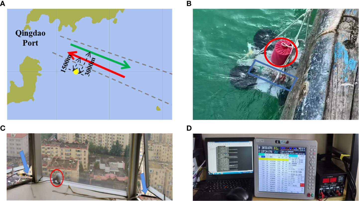
Figure 1 Sea trial system. (A) Submarine topographic map. The yellow circle marks the position of the submarine buoy. The middle part of the black dotted line is the channel. The red arrow is the direction of the inbound ship, which is about 1500 m away from the submarine buoy. The green arrow is the direction of the outbound ship, which is about 3000 m away from the submarine buoy. (B) Submersible buoys. The part in the red circle is the hydrophone part of the self-contained hydrophone, and the cylinder in the blue box is its data-sampling and processing system. (C) AIS signal receiving terminal. The part in the red circle is the GPS antenna, and the long black pole pointed by the blue arrow is the AIS signal antenna. (D) AIS data system.

2.2 Experimental data preprocessing

Data preprocessing is required to achieve better performance. The low-frequency analysis and recording (LOFAR) diagram is a basic time-frequency representation often used for localizing sources.

The short-time Fourier transform (STFT) can transform the raw signal into a LOFAR diagram using STFT. The time of the cloest point to the approach ($t_{CPA}$) was estimated based on the LOFAR diagram. After comparing $t_{CPA}$ with the AIS data, we labeled the LOAR diagram as an inbound or outbound ship.

By processing the experimental data, we found that the structures of the LOFAR diagrams of inbound and outbound ships are different. LOFAR diagrams of Figures 2A, B are the LOFAR diagrams of the same ship’s departure and arrival. In the experimental data, the interference fringes of the outbound ships generally bent down on the right side. In contrast, those of the inbound ships bent down on the left side. Owing to this difference, we used CNNs to extract features and classify inbound and outbound ships.

FIGURE 2

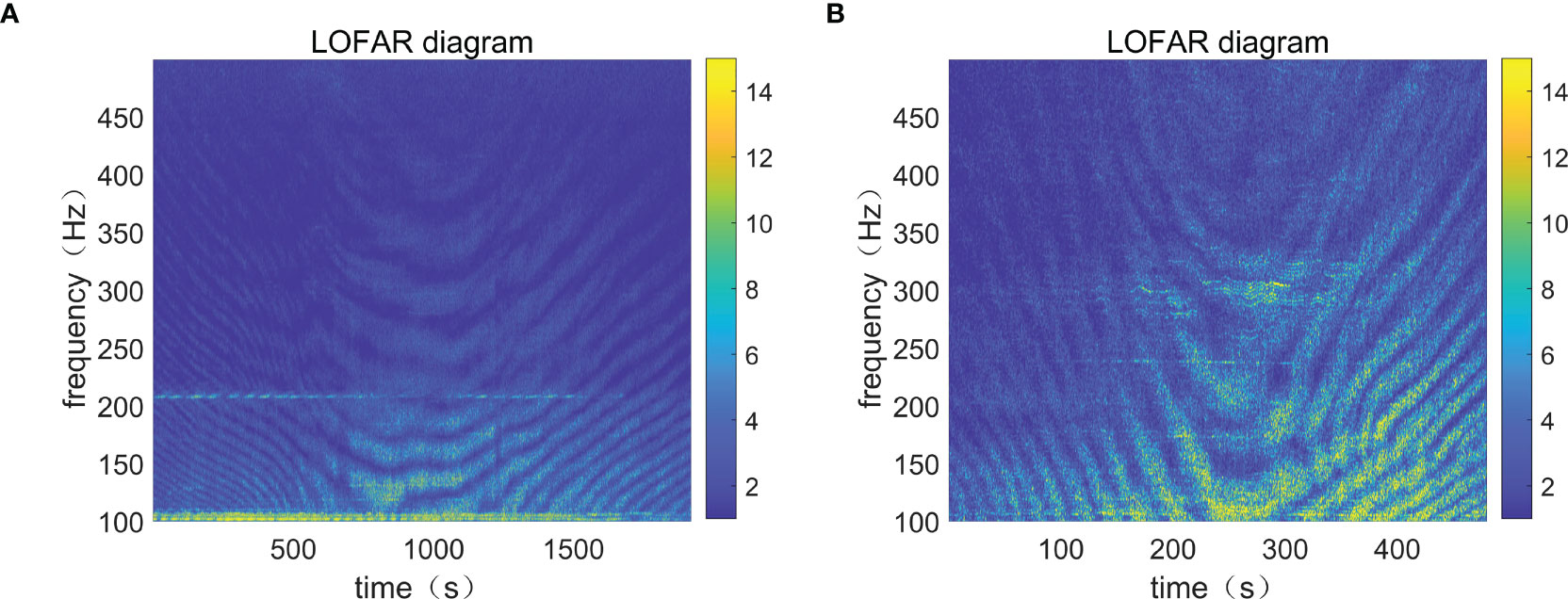
Figure 2 LOFAR diagrams of the same ship entering and leaving the port. (A) Inbound time-frequency diagram. (B) Outbound time-frequency diagram.

3 Method

This study proposed a method based on CNNs to classify inbound and outbound ships using a single scalar hydrophone on a shallow continental shelf. The flowchart is shown in Figure 3A. We used the STFT to transform the raw signal into a LOFAR diagram. The diagram was used as the input to the trained deep-learning models after edge detection to classify the ships.

FIGURE 3

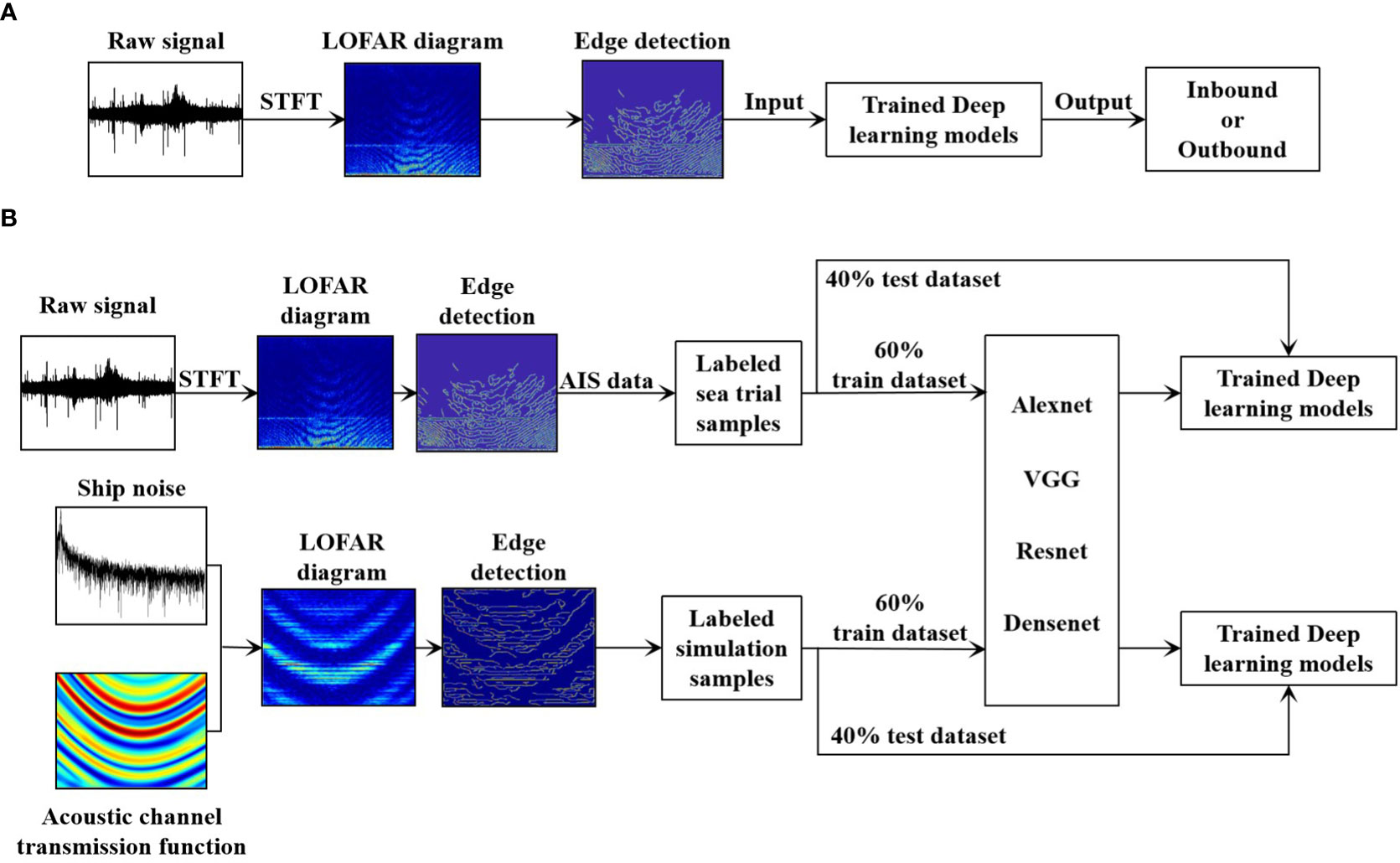
Figure 3 Ships classification algorithm flow chart. (A) Overall flow chart of ships classification algorithm. (B) Deep-learning models training flow chart.

Training deep-learning models require training datasets of various labeled samples. As the range at the closest point of approach, $r_{CPA}$, was relatively fixed in the experimental data, simulation data were also used during the training and validation steps. As shown in Figure 3B, both experimental and simulation data were used to train the models, which were tested with the experimental and simulation test sets, respectively.

3.1 Simulation data

The simulation was divided into three steps. First, building the ship radiated noise model and getting the ship radiated noise $s(\omega )$, and second, obtaining the channel transfer function $H(\omega )$ using the sound propagation calculation model Range-dependent acoustic model (RAM). Finally, the hydrophone reception signal is obtained by multiplying $H(\omega )$ and $s(\omega )$.

3.1.1 Ship noise simulation

Ship noise is mainly composed of a line spectrum and a continuous spectrum. Its mathematical model can usually be expressed as

$\begin{array}{ll}S(t)=[1+G(t)]\times S_x(t)+S_l(t)& (1)\end{array}$

The line spectrum component can be simulated by generating a series of sinusoidal signals, and its parameters can be set according to the following methods (He and Zhang, 2005).

(1) For line spectrum below 100 Hz, the fundamental frequency of shaft frequency line spectrum can be set as s, and the frequency of blade and harmonic line spectrum is mns Where $s$ is the propeller speed; the unit is turn/s; n is the number of propeller blades, and m is the harmonic number.

(2) The line spectrum with a frequency of 100–1000 Hz has no significant relationship with the ship’s speed but varies with the type of ship. K frequencies can be set without loss of generality.

The construction of the continuous spectral data was completed in three steps. First, we constructed the ship noise source level for different tonnages and speeds according to the empirical equation summarized by Ross (1976), as shown in Figure 4A. Next, we constructed an finite impulse response (FIR) filter with a specific frequency response using the LMS-adaptive algorithm, as shown in Figure 4B. Finally, a continuous spectrum of the radiated noise of the ship was obtained by inputting Gaussian white noise through the filter.

FIGURE 4

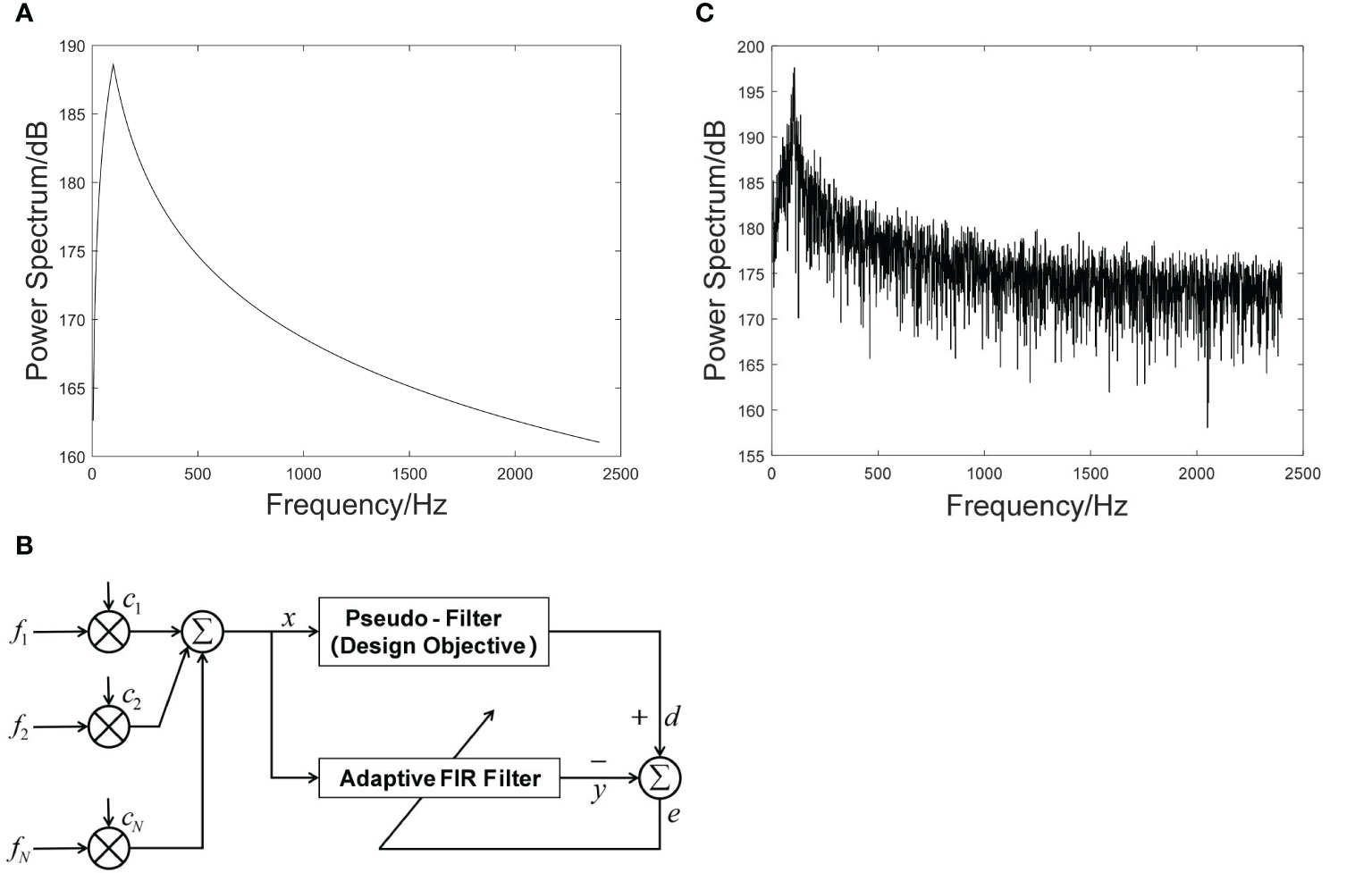
Figure 4 The ship’s radiated noise. (A) The ship noise source level. (B) Structure of FIR filter with specific frequency. (C) Power spectrum of ship’s radiated noise.

After adding a line spectrum to the continuous spectrum, the power spectrum of the radiated noise of the ship was obtained, as shown in Figure 4C.

3.1.2 Transfer function simulation

In this section, the underwater acoustic propagation software RAM is used to simulate the transfer function $H(\omega )$ of the channel (Collins, 1993).

The main environmental parameters for the simulation were as follows. The experimental sea area was off the coast of Qingdao, and the seabed terrain was a typical horizontal, slowly varying wedge seabed. Therefore, a wedge-shaped seafloor was used for the simulation. The sound velocity of the seabed is set as 1620 m·s^-1, the seabed density is 1.76 g·cm^-3, and the seabed attenuation is 0.3 dB·λ^-1. The sound velocity profile was obtained from the measured CTD data in the offshore waters of Qingdao on June 30, 2022. The acoustic source emission band was 200 – 400 Hz; the receiver depth was 26 m; the time of the closest point of approach ($t_{CPA}$)was 150 s; the range at the closest point of approach ($r_{CPA}$)was set to 1000 m; the sound source depth (d) was 5 m, and the motion speed (v) was 10 m/s. The 3D structure chart is shown in Figure 5A.

FIGURE 5

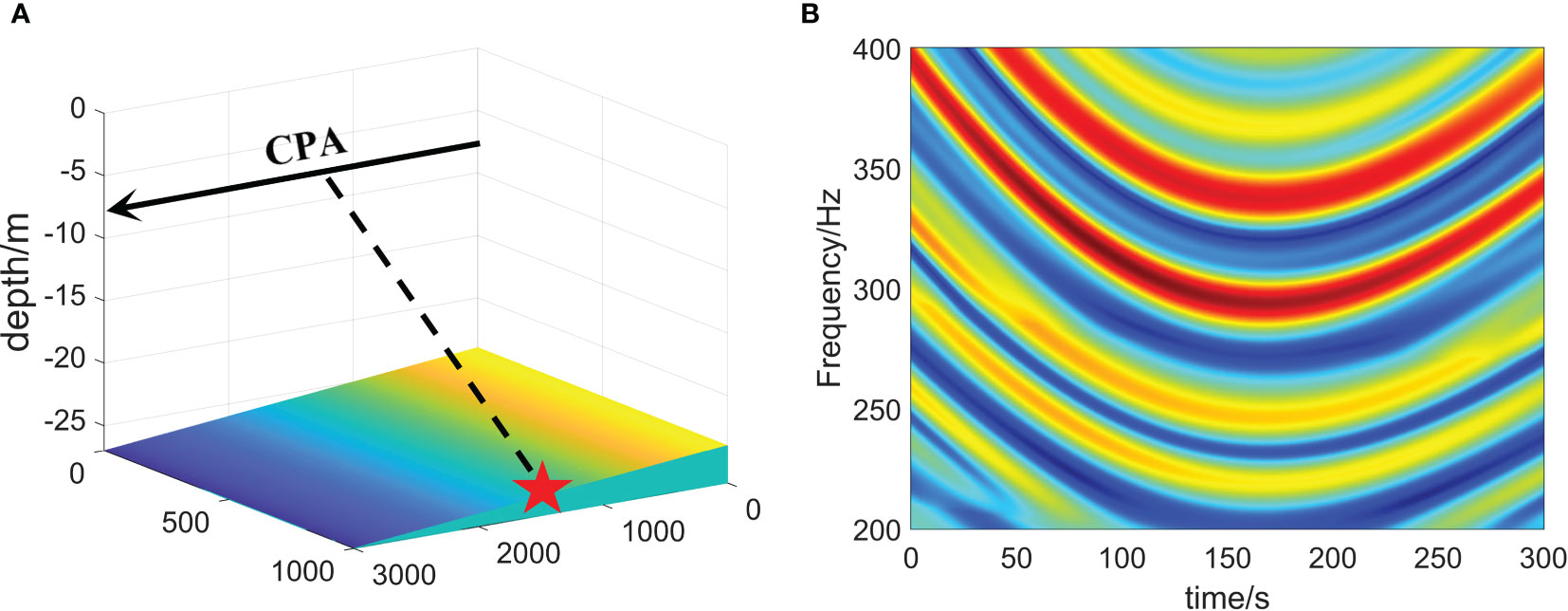
Figure 5 Simulation of transfer function. (A) 3D water depth distribution. (B) Time-frequency diagram of waveguide transfer function.

The spectrum received by the hydrophone is calculated every 2 s. After splicing, the time-frequency diagram, as shown in Figure 5B, is obtained. The transfer function $H(\omega )$ of the channel under different conditions is obtained by changing the parameters such as d, v, and $r_{CPA}$.

The spectrum of the radiated noise of the ship was multiplied by the transfer function spectrum, and the LOFAR diagram was obtained after splicing. As shown in Figure 6, the signal-to-noise ratio is set at 10 dB.

FIGURE 6

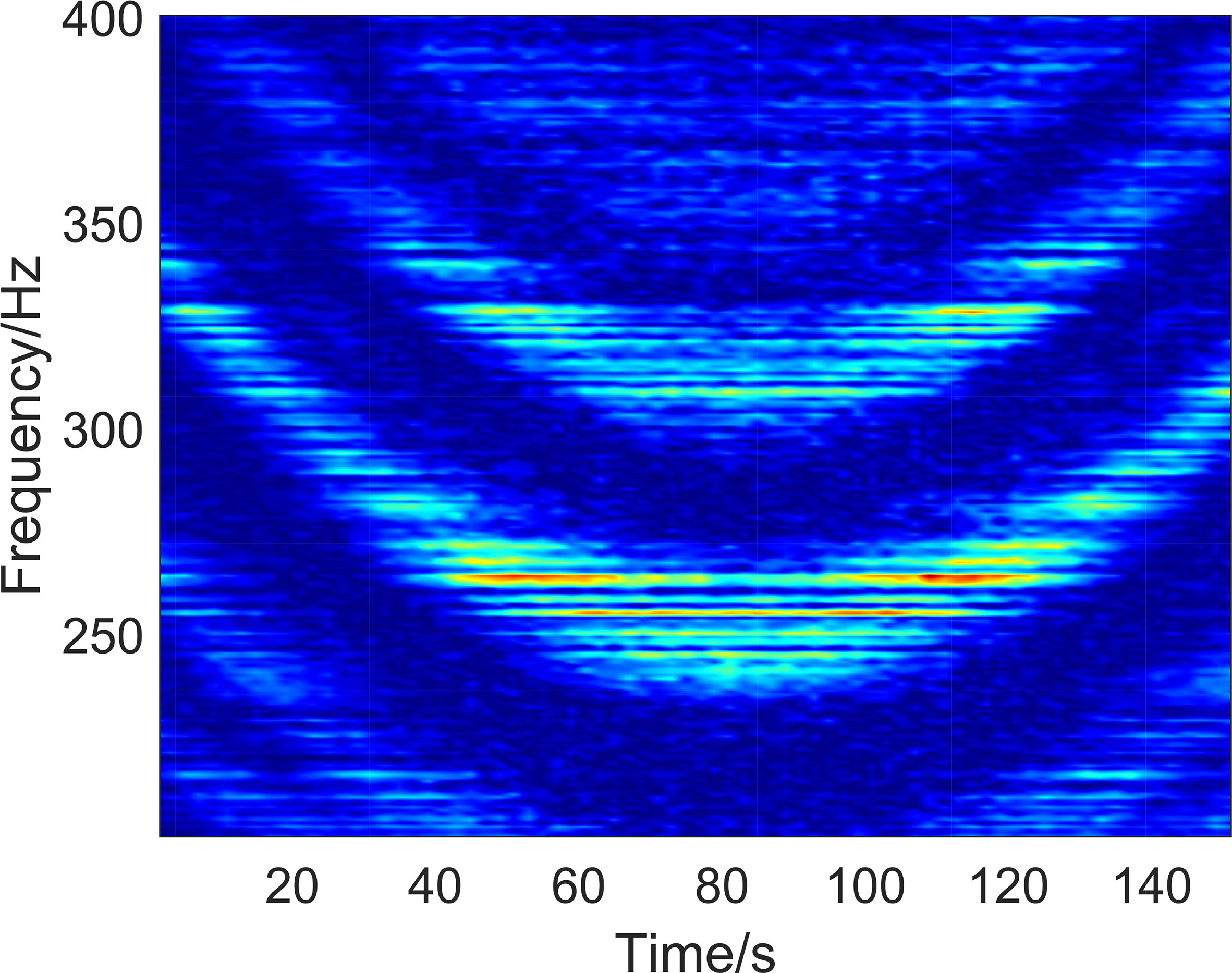
Figure 6 Time-frequency diagram of the received signal.

3.2 Network architecture

3.2.1 AlexNet

In 2012, Krizhevsky et al. proposed AlexNet, which realized a TOP5 error rate of 15.4% (The TOP5 error rate is the probability that, given an image, its label is not in the top five outcomes that the model considers most likely), and realized a deep convolutional neural network structure in a large-scale image dataset for the first time. AlexNet includes eight layers of transformations, including five convolution layers, two fully connected hidden layers, and one fully connected output layer (Krizhevsky et al., 2012), as shown in Figure 7. The network uses a rectified linear unit (ReLU) as a nonlinear mapping function, which makes the model converge more rapidly. The dropout mechanism was used to effectively reduce the overfitting problem to a certain extent, and the GPU replaced the CPU for calculations, significantly improving the training speed of the network.

FIGURE 7

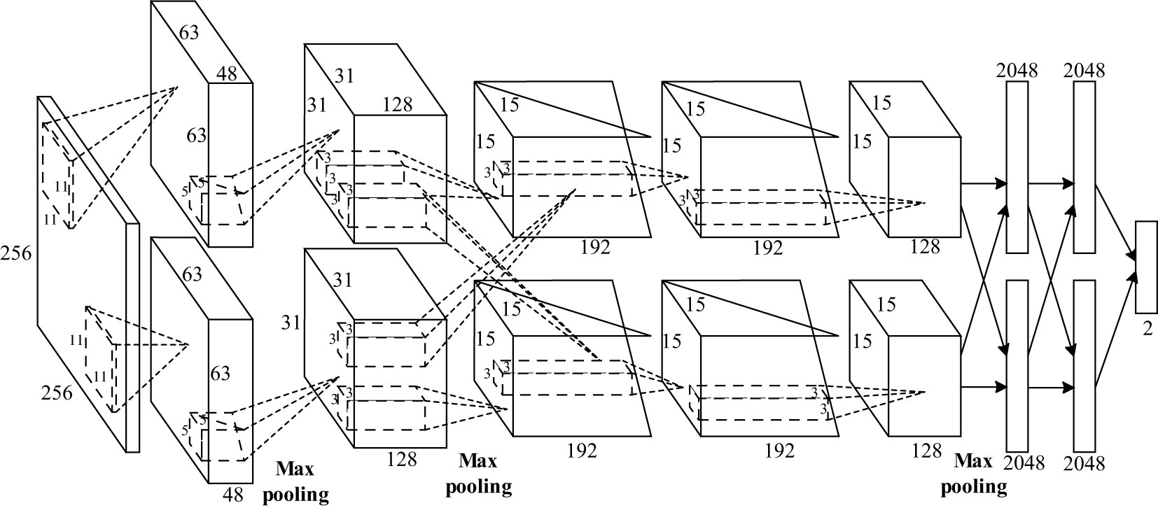
Figure 7 Structure of AlexNet.

3.2.2 VGG

Simonyan and Zisserman (2014) studied the depth of CNNs based on AlexNet, proved that increasing the depth of the network can affect its performance to a certain degree, and proposed the idea of building a depth model by reusing simple basic blocks. The network structure of the VGG is shown in Figure 8. The first part comprises convolution and convergence layers, and the second comprises a fully connected layer. The original VGG network has five convolution blocks, of which the first two blocks each have one convolution layer, and the last three blocks each contain two convolution layers. Because the network uses eight convolution layers and three fully connected layers, it is usually called VGG-11.

FIGURE 8

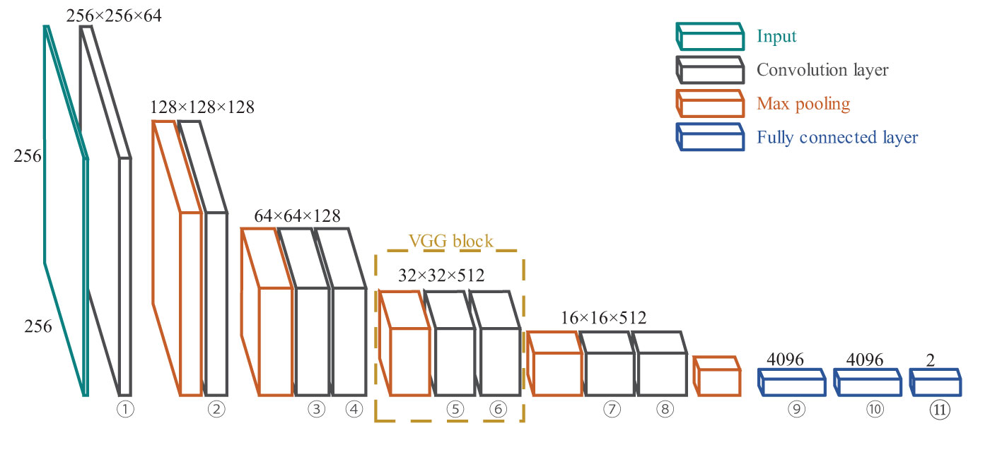
Figure 8 Network structure of VGG.

Compared to AlexNet, VGG uses a smaller convolution core and a deeper network structure. However, the increase in the network depth is limited. Many network layers leads to network degradation.

3.2.3 ResNet

Based on VGG, He et al. (2015) effectively solved the problem of decreasing the accuracy of the training set with the deepening of the network through the design of residual blocks.

The basic structure of the residual block is shown on the right side of Figure 9. The residual block changes the learning target to the difference between target values H (X) and x, called the residual. Residual mapping is often easier to optimize. Through the design of the residual block, some neural network layers can be artificially created to skip the connection of neurons in the next layer, thus weakening the strong connections between each layer.

FIGURE 9

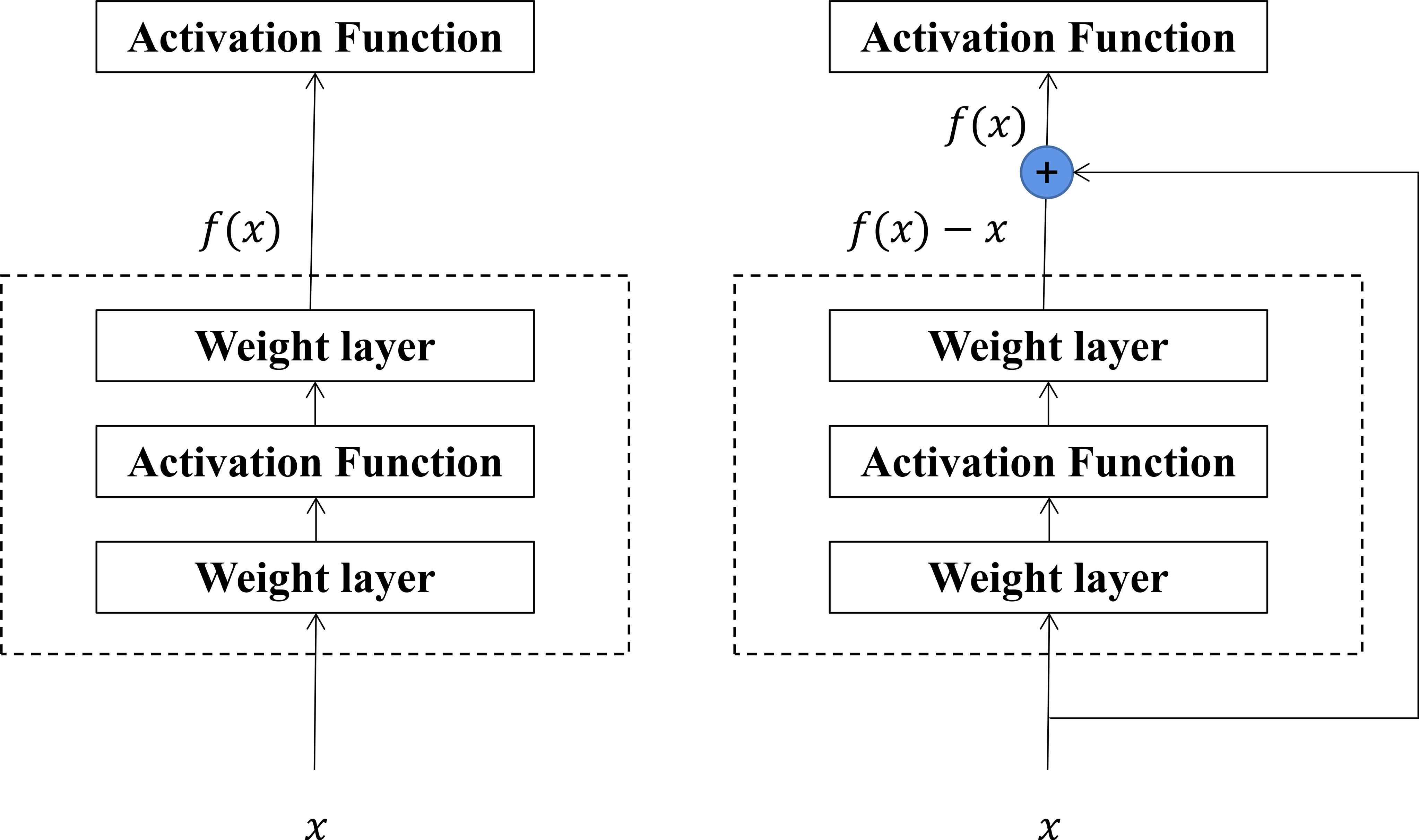
Figure 9 Structure of residual block.

3.2.4 DenseNet

In 2017, Huang et al. proposed DenseNet based on ResNet. However, unlike ResNet, DenseNet proposed a more radical dense connection mechanism where all layers are interconnected (2017). Specifically, each layer accepts all the layers in front of it as its additional input, as shown in Figure 10, which can achieve feature reuse and improve efficiency.

FIGURE 10

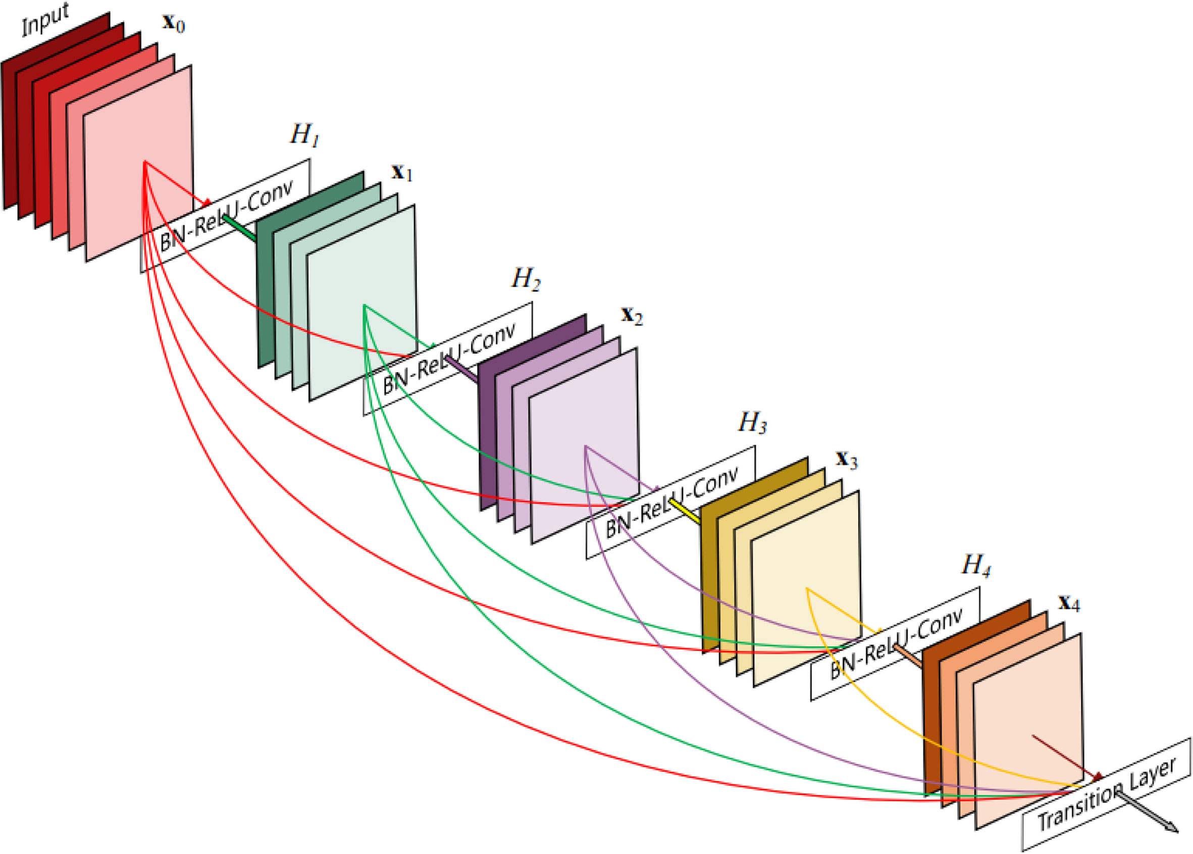
Figure 10 Dense connection structure.

3.3 Training CNNs

3.3.1 Input data preprocessing

As shown in Figure 11, before inputting in the CNNs, all of the LOFAR diagrams were resampled to 256×256 for the reduction of the computation, smoothed by mean filtering to reduce salt-and-pepper noise, and the Canny operator detected edges for better performance. The experimental and simulation data were split into training and test sets at the same ratio. The ratio of the training set to the test set is 40%:60%.

FIGURE 11

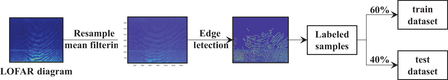
Figure 11 Input data preprocessing flow chart.

3.3.2 Network training

The implementation of the neural networks mentioned in Section 3.2 was done in Python 3 using the open-source Pytorch (Paszke et al., 2019). The network was trained for 100 and 20 epochs on the sea trial and simulation datasets, respectively. The batch size was set to 32. An Intel Core i7-9700 3.00 GHz CPU trained the networks. The final trained model could complete the classification of 128 samples in 8.53 s.

4 Results

4.1 Accuracy and train loss

The results for the simulation training dataset are presented in Figure 12. From the perspective of training loss, ResNet and DenseNet declined rapidly, whereas AlexNet and VGG declined relatively slowly. From the training set’s perspective, the four networks’ training accuracy reached 100%, but that of AlexNet and VGG fluctuated significantly. For the test dataset, the final test accuracies of AlexNet, VGG, ResNet, and DenseNet were 99.49%, 100%, 100%, and 100%, respectively. AlexNet and VGG exhibited larger fluctuations.

FIGURE 12

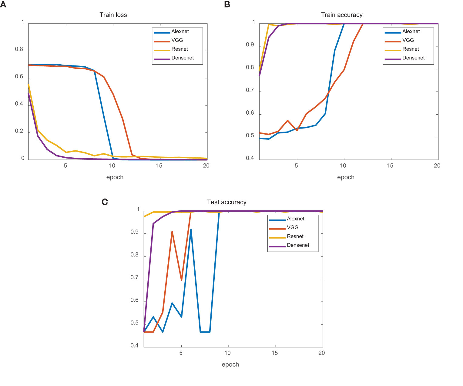
Figure 12 Simulation data classification results. (A) Train loss of four networks. (B) Train accuracy of four networks. (C) Test accuracy of four networks. AlexNet is the blue line. VGG is the red line. ResNet is the yellow line. DenseNet is the purple line.

The results for the experimental dataset are illustrated in Figure 13. Compared to the simulation dataset, the experimental dataset fluctuated greatly, which may be due to the influence of marine environmental noise (such as the calls of marine organisms) in individual samples. From the perspective of the test dataset, the final test accuracies of AlexNet, VGG, ResNet, and DenseNet were 90.63%, 95.51%, 96.63%, and 99.22%, respectively. AlexNet and VGG fluctuated less, but their final test-set accuracies were lower. ResNet fluctuated more; however, its final test set accuracy was higher. DenseNet fluctuated less but had the highest final test set accuracy.

FIGURE 13

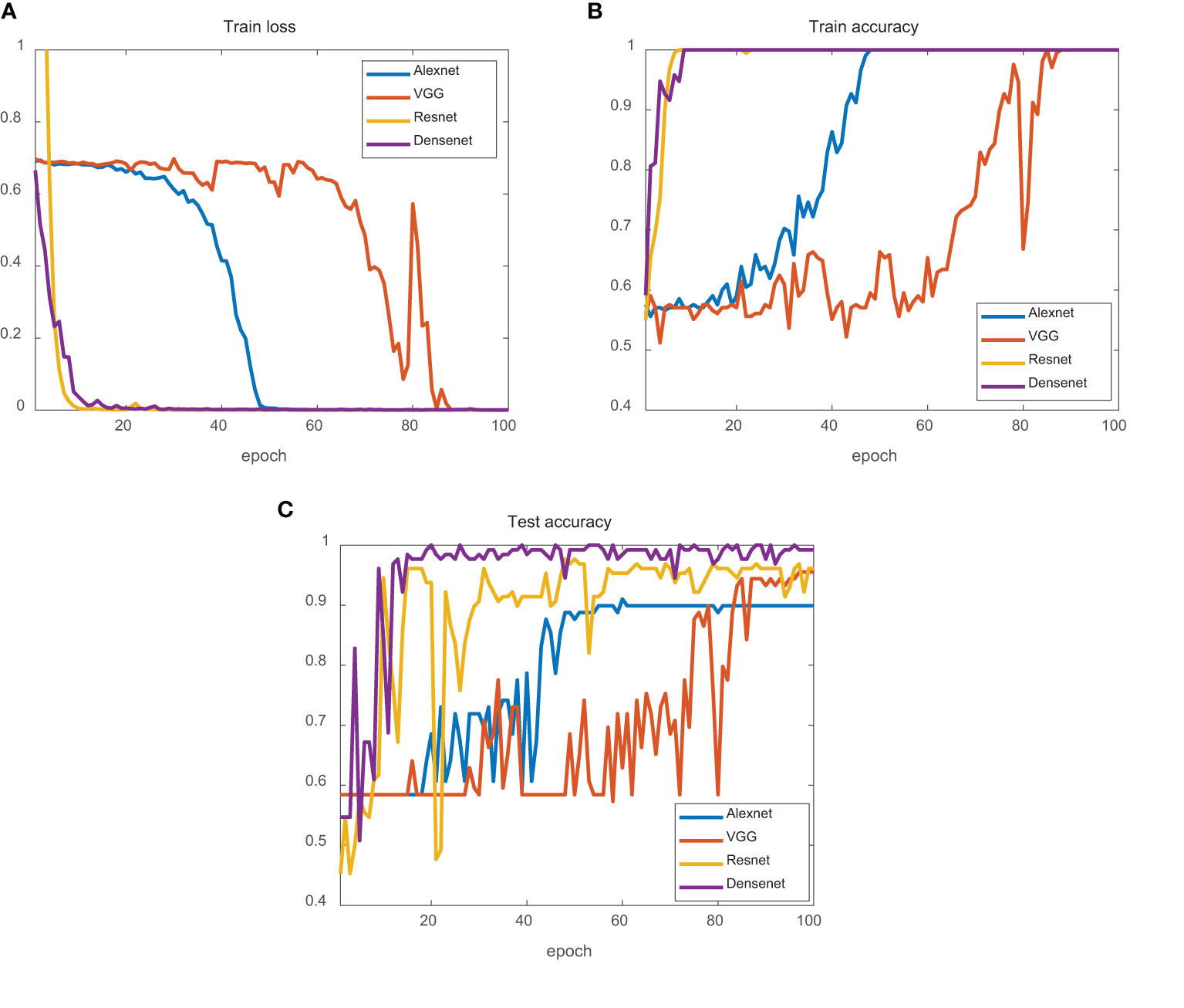
Figure 13 Experimental data classification results. (A) Train loss of four networks. (B) Train accuracy of four networks. (C) Test accuracy of four networks. AlexNet is the blue line. VGG is the red line. ResNet is the yellow line. DenseNet is the purple line.

Overall, ResNet and DenseNet performed better than AlexNet and VGG on both the simulation and experimental datasets, possibly because they used a residual block design with a deeper network structure. In the experimental dataset, the stability of DenseNet was better than that of ResNet, and the final test set accuracy of DenseNet was higher, which may be because DenseNet adopts a denser connection mechanism.

4.2 Confusion matrixes

Table 1 presents the confusion matrices of the four networks trained using the experimental datasets. Each column represents a prediction, and each row represents the true label of the data. Among the 128 inbound and outbound ships, AlexNet mistakenly judged three inbound ships as outbound and nine outbound ships as inbound. The VGG mistakenly judged one inbound ship as outbound and five outbound ships as inbound. ResNet recognized 70 outbound ships and 54 diagrams from 58 test diagrams of inbound ships. DenseNet outperformed the other three CNNs and recognized all 58 inbound ships and 68 diagrams from 70 testing diagrams of outbound ships. DenseNet offers a reliable method for classifying inbound and outbound ships.

TABLE 1

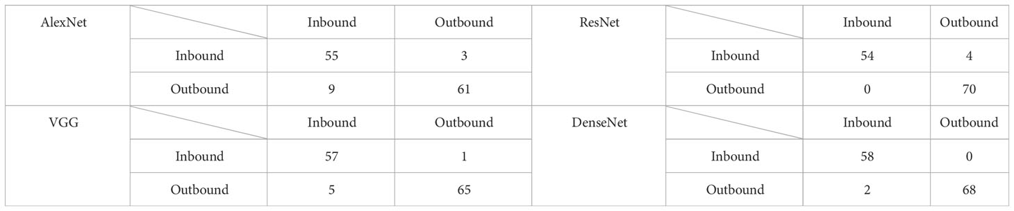
Table 1 Confusion matrixes of four networks trained by experimental datasets.

5 Analysis of physical principles

This study introduced the concept of a generalized waveguide invariant to analyze the reasons for the differences in the interference fringe structures of inbound and outbound ships. Based on the conventional definition of waveguide invariance, the generalized waveguide invariant considers the effect of azimuth change on the waveguide invariant $\beta$ and derives a new definition equation.

Assuming that the sound source moves along a straight line and its track does not pass through the receiver, the movement of the sound source will not only cause a change in the sound propagation path distance with time but also cause a change in the azimuth angle with time.

In Figure 14, the orange circle represents the receiver’s position, the blue rectangle represents the sound source, v represents the sound source’s moving speed, $v_{\tau }$ and $v_n$ the radial and tangential velocities, respectively, and $\theta$ represents the azimuth.

FIGURE 14

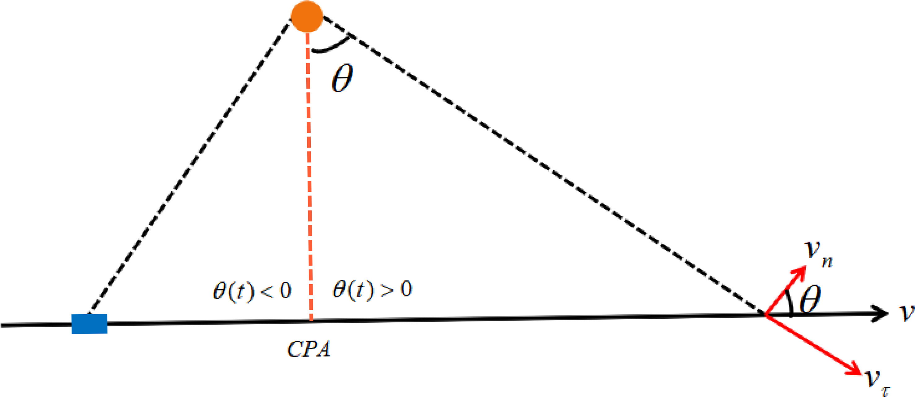
Figure 14 Schematic of sound source moving along a straight line without passing the receiver.

In this case, the waveguide-invariant $\beta$ was related to the distance and azimuth of the sound propagation path. Based on the definition equation $\beta =\frac{r}{\omega }\frac{d\omega }{dr}$ of the conventional waveguide invariant, the definition equation of the generalized waveguide invariant is derived as shown in Equation 2.

$\begin{array}{ll}\beta =\frac{r}{\omega }\frac{d\omega }{dr}=-\frac{s_{p,mn}\mathit{(}\omega ,\theta ,r\mathit{)}+\frac{\partial }{\partial \theta }\{\frac{\mathbf{1}}{r}{\int }_0^r{s}_{p,mn}(\omega ,\theta ,r\text{'})dr\text{'}\}cot\theta }{\frac{\mathbf{1}}{r}{\int }_0^r{s}_{g,mn}(\omega ,\theta ,r\text{'})dr\text{'}}& (2)\end{array}$

In Equation 2, the first term of the molecule contributes to the change in distance along the sound propagation path, and the second term corresponds to the change in azimuth. When the sound source is close to the nearest point and azimuth $\theta \to 0$, there is a singularity in the waveguide invariants’ values. When the distance between the sound source and the receiver is far enough, the azimuth change $\theta$ is very weak. β is mainly determined by the first term of Equation 2, and the influence of azimuth on waveguide invariants can be ignored. The first term in Equation 2 is a classical waveguide invariant expression. After adding the second term, the waveguide invariant β is related to the distance and the azimuth variation term between the sound source and the receiver.

According to the theory of generalized waveguide invariants, the value of waveguide invariants changes abruptly before and after the target ship passes the nearest point, which causes asymmetric interference fringes on the time-frequency diagram. Furthermore, the directions of the inbound and outbound ships are opposite; therefore, their interference fringe structures show different characteristics: one is high on the left and low on the right, and the other is high on the right and low on the left.

6 Conclusion

Here, we first found that the spectrum interference structure of the acoustic signal received by a single hydrophone is asymmetric in sea trial experimental data. Then we used this feature to classify inbound and outbound ships using a single hydrophone through CNNs and explained the physical principle through generalized waveguide invariants.

This method overcame the idea that single-scalar hydrophones can only be used for ranging, and not direction-finding. This algorithm classified the direction of the target ship using only a single-scalar hydrophone. However, at this stage, it was only possible to determine approximately whether a ship was inbound or outbound, and a more detailed course judgment could not be completed. When the seabed topography was known for specific sea areas, this method could achieve more detailed course discrimination and complete the positioning of the target ship or underwater target. This algorithm could achieve more comprehensive sea area monitoring by combining ls-ssdd-v1.0 and official-ssdd with SAR ship classification and identification. This issue should be addressed in future studies.

Data availability statement

The raw data supporting the conclusions of this article will be made available by the authors, without undue reservation.

Author contributions

Conceptualization, DZG. Methodology, DZG and DDG. Software, DDG and ZC. Experiment, YL, XZ, and DDG. Writing, review, and editing, DZG, DDG, XZ, WS, and XL. All authors contributed to the article and approved the submitted version.

Funding

The word was supposed by the National Natural Science Foundation of China (Grant Nos. 12274385, 11874331, 12004359, 52001296).

Conflict of interest

The authors declare that the research was conducted in the absence of any commercial or financial relationships that could be construed as a potential conflict of interest.

Publisher’s note

All claims expressed in this article are solely those of the authors and do not necessarily represent those of their affiliated organizations, or those of the publisher, the editors and the reviewers. Any product that may be evaluated in this article, or claim that may be made by its manufacturer, is not guaranteed or endorsed by the publisher.

References

Baggeroer A. B., Kupennan W. A., Mikhalevsky P. N. (1993). An overview of matched field methods in ocean acoustics. IEEE J. Oceanic Eng. 18 (4), 401–424. doi: 10.1109/48.262292

CrossRef Full Text | Google Scholar

Carter G. C. (1981). Time delay estimation for passive sonar signal processing. IEEE Trans. Acoustics Speech Signal Process. 29 (3), 463–470. doi: 10.1109/TASSP.1981.1163560

CrossRef Full Text | Google Scholar

Chi J., Gao D. Z., Zhang X. G., Zhang X. Y., Wang Z. Z. (2021). Motion parameter estimation of multitonal sources with a single hydrophone[J]. JASA Express Lett. 1 (1), 016006. doi: 10.1121/100003368

PubMed Abstract | CrossRef Full Text | Google Scholar

Cho C., Song H. C., Hodgkiss W. S. (2016). Robust source-range estimation using the array/waveguide invariant and a vertical array. J. Acoustical Soc. America 139 (1), 63~69. doi: 10.1121/1.4939121

CrossRef Full Text | Google Scholar

Clay C. S. (1987). Optimum time domain signal transmission and source location in a waveguide. J. Acoustical Soc. America 81 (3), 660–664. doi: 10.1121/1.394834

CrossRef Full Text | Google Scholar

Cockrell K. L., Schmidt H. (2010). Robust passive range estimation using the waveguide invariant. J. Acoustical Soc. America 127 (5), 2780. doi: 10.1121/1.3337223

CrossRef Full Text | Google Scholar

Collins M. D. (1993). A split-step pade solution for the parabolic equation method. Acoust Soc. Am(S0001-4966) 93 (4), 1736–1742. doi: 10.1121/1.406739

CrossRef Full Text | Google Scholar

Gao D. Z., Kang D. X., Song W. H., Li X. L., Li Y. Z. (2022). Generalized waveguide invariant. Tech. Acoustics 41 (03), 403–411. doi: 10.16300/j.cnki.1000-3630.2022.03.014

CrossRef Full Text | Google Scholar

He Z. Y., Zhang Y. P. (2005). Modeling and simulation research of ship-radiated noise. Audio Eng. 12), 52–55. doi: 10.16311/j.audioe.2005.12.014

CrossRef Full Text | Google Scholar

He K., Zhang X. Y., Ren S. Q., Sun J. (2015). Deep residual learning for image recognition. In IEEE Conference on Computer Vision and Pattern Recognition (CVPR), 770–778. doi: 10.1109/CVPR.2016.90

CrossRef Full Text | Google Scholar

Huang G., Liu Z., van der Maaten L., Weinberger K. Q. (2017). Densely connected convolutional networks. IEEE Conf. Comput. Vision Pattern Recognition (CVPR). doi: 10.1109/CVPR.2017.243

CrossRef Full Text | Google Scholar

Jauffret C., Bar-Shalom Y. (1990). Track formation with bearing and frequency measurements in clutter. IEEE Trans. Aerospace Electronic Syst. 26 (6), 999–1010. doi: 10.1109/7.62252

CrossRef Full Text | Google Scholar

Krizhevsky A., Sutskever I., Hinton G. (2017). ImageNet classification with deep convolutional neural networks. Communications of the ACM 60 (6), 84–90. doi: 10.1145/3065386

CrossRef Full Text | Google Scholar

Li Q. L., Song W. H., Gao D. Z., Chi J., Gao D. Y. (2022). Passive localization of shallow sea target using interferogram. Acta Acustica 47 (05), 625–633. doi: 10.15949/j.cnki.03710025.2022.05.012

CrossRef Full Text | Google Scholar

Maranda B. H., Fawcett J. A. (1991). Detection and localization of weak targets by space-time integration. IEEE J. Oceanic Eng. 16 (2), 189–194. doi: 10.1109/48.84135

CrossRef Full Text | Google Scholar

Nardone S. C., Lindgren A. G., Gong K. F. (1984). Fundamental properties and performance of conventional bearings-only target motion analysis. Automatic Control IEEE Trans. 29 (9), 775~787. doi: 10.1109/TAC.1984.1103664

CrossRef Full Text | Google Scholar

Paszke A., Gross S., Massa F., Lerer A., Chintala S. (2019). Pytorch: an imperative style, high-performance deep learning library. Adv Neural Inf Process Syst. 32, 1912.01703. doi: 10.48550/arXiv.1912.01703

CrossRef Full Text | Google Scholar

Ross D. (1976). Mechanics of underwater noise (New York: Pergamon Press).

Google Scholar

Simonyan K., Zisserman A. (2014). Very deep convolutional networks for Large-scale image recognition. CoRR, abs/1409.1556. doi: 10.48550/arXiv.1409.1556

CrossRef Full Text | Google Scholar

Song H. C., Cho C. (2015). The relation between the waveguide invariant and array invariant. J. Acoustical Soc. America 138 (2), 899~903. doi: 10.1121/1.4927090

CrossRef Full Text | Google Scholar

Song H. C., Cho C. (2017). Array invariant-based source localization in shallow water using a sparse vertical array. J. Acoustical Soc. America 141 (1), 183~188. doi: 10.1121/1.4973812

CrossRef Full Text | Google Scholar

Song H. C., Cho C., Byun G., Kim J. S. (2017). Cascade of blind deconvolution and array invariant for robust source-range estimation. J. Acoustical Soc. America 142 (4), 3270~3273. doi: 10.1121/1.4983303

CrossRef Full Text | Google Scholar

Thode A. M. (2000). Source ranging with minimal environmental information using the virtual receiver and waveguide invariant concepts. J. Acoustical Soc. America 107 (5), 2867. doi: 10.1121/1.1289409

CrossRef Full Text | Google Scholar

Xu X. W., Zhang X. L., Zhang T. W. (2022). Lite-YOLOv5: a lightweight deep learning detector for on-board ship detection in Large-scene sentinel-1 SAR images. Remote Sens. 14 (4), 1018–1018. doi: 10.3390/rs14041018

CrossRef Full Text | Google Scholar

Zhang T., Zhang X., Ke X., Liu C., Xu X., Zhan X., et al. (2021). HOG-ShipCLSNet: a novel deep learning network with HOG feature fusion for SAR ship classification. IEEE Trans. Geosci. Remote Sens. 60, 1–22. doi: 10.1109/TGRS.2021.3082759

CrossRef Full Text | Google Scholar