Hybrid quantum-classical convolutional neural network for phytoplankton classification

1 Introduction

Phytoplankton is the most important primary producer in the aquatic ecosystem. As the main supplier of dissolved oxygen in the ocean, phytoplankton plays a vital role in the energy flow, material circulation and information transmission in the marine ecosystem (Barton et al., 2010; Gittings et al., 2018). The species composition and abundance of phytoplankton are key factors in marine ecosystem dynamics, exerting a direct influence on global environment change. As such, much attention has been paid to the identification and classification of phytoplankton (Zheng et al., 2017; Pastore et al., 2020; Fuchs et al., 2022).

With the rapid development of imaging devices for phytoplankton (Owen et al., 2022), a huge number of phytoplankton images can now be collected in a short time. However, it has become impossible to classify and count these images using traditional manual methods, i.e. expert-based methods. To increase the efficiency of processing these images, machine learning methods has been introduced, including support vector machine (Hu and Davis, 2005; Sosik and Olson, 2007), random forest (Verikas et al., 2014; Faillettaz et al., 2016), k-nearest neighbor (Glüge et al., 2014), and artificial neural network (Mattei et al., 2018; Mattei and Scardi, 2020). In particular, convolutional neural network (CNN), which achieves state-of-the-art performance on image classification, has become widely used in this field in recent years. A variety of CNN-based architectures have been proposed to identify and classify phytoplankton with high efficiency and precision (Dai et al., 2017; Cui et al., 2018; Wang et al., 2018; Fuchs et al., 2022).

To conduct large-scale research on marine phytoplankton, more powerful computational resources are desired to ensure the success of machine learning methods for handling the overwhelmingly increasing volume of data. Along with the remarkable progress in the field of quantum computing (Arute et al., 2019; Zhong et al., 2020; Bharti et al., 2022; Madsen et al., 2022), quantum machine learning (QML) has emerged as a potential solution for large-scale data processing (Biamonte et al., 2017). There is a growing consensus that even the near-term NISQ (noisy intermediate-scale quantum) devices may find advantageous applications (Preskill, 2018), one of which is the quantum neural network (QNN) (Jeswal and Chakraverty, 2019; Kwak et al., 2021). The QNN takes the parameterized quantum circuit (PQC) as a learning model (Benedetti et al., 2019), and can be naturally extended to a quantum deep neural network with the flexible multilayer architecture. The quantum convolutional neural network (QCNN) is a typical model of quantum deep neural networks that has recently received a lot of attention and achieved significant developments. QCNN has demonstrated its success in processing both quantum and classical data, including quantum many-body problems (Cong et al., 2019), identification of high-energy physics events (Chen et al., 2022), COVID-19 prediction (Houssein et al., 2022) and MNIST dataset classification (Oh et al., 2020).

In this work, we explore the potential of QCNN for performing phytoplankton classification. There are two typical architectures of QCNN: the fully quantum parameterized QCNN (Cong et al., 2019) and the hybrid quantum-classical CNN (Liu et al., 2021). Due to the large size of phytoplankton images and the limited number of qubits and quantum operations available on current quantum devices, it is currently impractical to learn the images using fully quantum parameterized QCNN. Therefore, we adopt the hybrid quantum-classical convolutional neural network (QCCNN) architecture to achieve good multi-classification of the phytoplankton dataset. QCCNN integrates the PQC into the classical CNN architecture by replacing the classical feature map with the quantum feature map. This makes QCCNN friendly to current NISQ devices in terms of both the number of qubits and circuit depths, while retaining important features of classical CNN, such as nonlinearity and scalability (Liu et al., 2021).

Moreover, the QCCNN may face challenges such as the barren plateau problem (i.e. vanishing gradient) and degradation problem (i.e. saturated accuracy with increasing depth) (Deng, 2021). To address these issues, we further propose a hybrid quantum-classical residual network (QCResNet) that incorporates a residual architecture to enhance the QCCNN’s performance.

It is worth noting that the visual transformer has recently achieved remarkable performance in image processing (Dosovitskiy et al., 2020) by identifying long-range dependencies and obtaining global information. Its success has led to its application in classifying plankton datasets (Baek et al., 2022; Dagtekin and Dethlefs, 2022; Kyathanahally et al., 2022; Shao et al., 2022). In the future, it will be intriguing to develop quantum visual transformer models based on the quantum self-attention mechanism (Li et al., 2022; Shi et al., 2023; Zhao et al., 2022), and explore their potential for phytoplankton classification.

The main contribution of this work is as follows:

(1) For the first time, the feasibility of using quantum deep neural networks for phytoplankton classification is demonstrated. This represents a concrete example of the application of quantum machine learning methods in the field of marine science.

(2) Several specific architectures for QCCNN and QCResNet are developed, which are accessible on near-term NISQ devices. Particularly, the QCResNet architecture is proposed to enhance the QCCNN’s performance. These models are versatile and can be directly applied to other image classification tasks.

(3) The QCCNN and QCResNet models demonstrate exceptional performance in phytoplankton classification compared to template CNN and ResNet models. Moreover, the impact of PQC’s expressibility and entangling capability on QCCNN’s performance is explored.

The rest of the paper is organized as follows. Section 2 provides introduction to the preliminaries of QNN. In section 3, we discuss the architectures of QCCNN and QCResNet. Section 4 describes the phytoplankton dataset used in the experiment. Section 5 presents the experimental results, including the performance of QCCNN and QCResNet, as well as the impact of ansatz circuit on QCCNN’s performance. Finally, conclusions are given in section 6.

2 Quantum neural network

QNN is a type of variational quantum algorithm, which is also the hybrid quantum-classical algorithm. Typically, QNN consists of four parts: data encoding, forward transformation performed by the ansatz, quantum measurement and parameter optimization routine, as illustrated in Figure 1. It’s worth noting that the first three parts are implemented on the quantum device, while the optimization routine is executed on the classical computer, which then feeds the updated parameters back into quantum device.

FIGURE 1

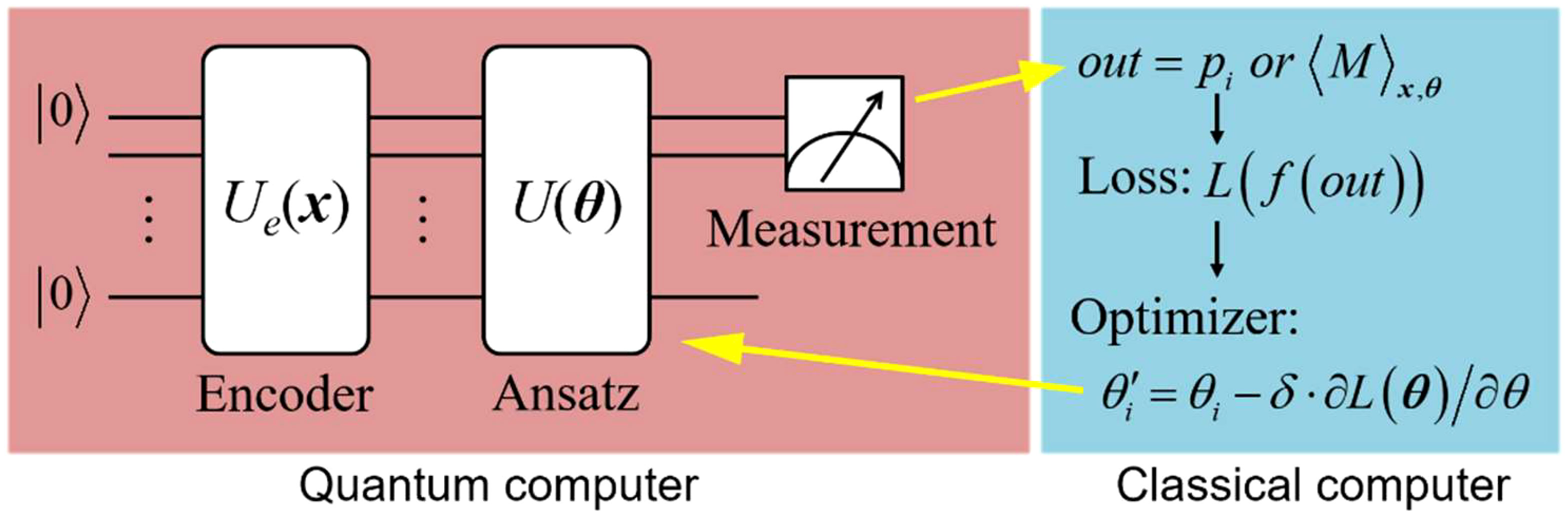
Figure 1 Architecture of QNN model. QNN is a hybrid quantum-classical algorithm. The forward transformation is implemented by the quantum computer, while the optimization of parameters is done by the classical computer.

Data encoding is the process of embedding classical data into quantum states by applying a unitary transformation, i.e.$|\mathit{x}\rangle =U_e{|0\rangle }^{\otimes n}$where $|\mathit{x}\rangle$is proportional to the data vector x. Data encoding can be regarded as a quantum feature map that maps the data space to the quantum Hilbert space (Schuld and Killoran, 2019). QNNs leverage this exponentially large Hilbert space as the feature space, making it extremely difficult to simulate using classical resources (Havlíček et al., 2017). One of the most commonly used encoding method in QNN is the angle encoding. It embeds classical data into the rotation angles of the quantum rotation gates. For example, given a normalized data vector $\mathit{x}={(x_1,\dots x_N)}^T$ with $x_i\in [0,1)$ , angle encoding can embed it into

$\begin{array}{ll}{R}_y^{\otimes N}(\mathit{x}){|0\rangle }^{\otimes N}=\underset{i=1}{\overset{N}{\otimes }}\left(\cos \frac{x_i}{2}|0\rangle +\sin \frac{x_i}{2}|1\rangle \right),& (1)\end{array}$

where R_y is the rotation gate about the $\widehat{y}$ axes, i.e. $R_y(x_i)=\left[\cos \frac{x_i}{2},-\sin \frac{x_i}{2};\sin \frac{x_i}{2},\cos \frac{x_i}{2}\right]$ . For more information on data encoding strategies, please refer to (Hur et al., 2022).

The ansatz can be seen as a quantum analogue of feedforward neural network, which utilizes the quantum unitary transformation to implement the feature map of data. Essentially, the ansatz is a PQC with adjustable quantum gates. These adjustable parameters are optimized to approximate the target function that maps features into different domains representing different classes. Therefore, the structure of ansatz circuit plays a crucial role in specific learning tasks. In most cases, the hardware-efficient ansatz is adopted in QNN, which uses a limited set of quantum gates and a particular qubit connection topology that is specific to the quantum devices on hand. The gate set usually contains three single-qubit gates and one two-qubit gates. An arbitrary single-qubit gate can be expressed as a combination of rotation gates about the $\widehat{x}$ , and $\widehat{z}$ axes. For example, using the X-Z decomposition, a single-qubit gate can be represented as

$\begin{array}{ll}{U}_{1q}(\alpha ,\beta ,\gamma )=R_x(\alpha )R_z(\beta )R_x(\gamma ),& (2)\end{array}$

where α, β, and γ are the rotation angles. The two-qubit gates are utilized to create entanglement between qubits. There are fixed two-qubit gates without adjustable parameters, such as the CNOT gate, and the ones with adjustable parameters, such as the controlled R_x(θ) and R_z(θ) gates. A comprehensive discussion of the properties of different ansatz circuits is presented in (Sim et al., 2019).

Quantum measurement produces an output value that can be used as a prediction for the data. The measurement operation corresponds to a Hermitian operator M, which can be decomposed as $M={\displaystyle {\sum }_i{\lambda }_i|i\rangle \langle i|}$ , where ${\lambda }_i$ is the ith eigenvalue and $|i\rangle$ is the corresponding eigenvector. When a measurement is performed, the quantum state $|\psi \rangle$ will collapse to one of the eigenstates $|i\rangle$ with a probability $p_i={\left|\langle i|\psi \rangle \right|}^2$. Then, the expectation value of the measurement outcome is

$\begin{array}{ll}\langle M\rangle ={\displaystyle {\sum }_i{\lambda }_i·p_i}={\displaystyle {\sum }_i{\lambda }_i{\left|\langle i|\psi \rangle \right|}^2}.& (3)\end{array}$

The most fundamental measurement outcomes are the probabilities $\left\{p_i\right\}$ and the expectation $\langle M\rangle$ . The commonly used measurement in quantum computing is the computational basis measurement, also known as the Pauli-Z measurement, with the Hermitian operator

$\begin{array}{ll}{\sigma }_z=(+1)|0\rangle \langle 0|+(-1)|1\rangle \langle 1|.& (4)\end{array}$

When performing the σ_z measurement, a qubit will collapse to the state $|0\rangle$ ($|1\rangle$) with the probability. $p_0={\left|\langle 0|\psi \rangle \right|}^2$($p_1={\left|\langle 1|\psi \rangle \right|}^2$), and the corresponding eigenvalue is +1 (−1). The expectation value $\langle {\sigma }_z\rangle$ is a value within the range [-1, 1]. Due to the collapse principle of quantum measurement, in practice the probability and the expectation value are estimated using s samples of measurement, where s is known as the number of shots.

Optimization routine is used to update the parameters of the ansatz circuit. These parameters correspond to the adjustable rotation angles of gates and are updated based on the data. Optimizing the parameters θ is in fact the process of minimizing the loss function L(θ). Similar to classical models, QNN can use various loss functions such as mean squared error loss and cross-entropy loss. For example, the multi-category cross-entropy loss can be expressed as

$\begin{array}{ll}L(\theta )=-\frac{1}{N}{\displaystyle \sum _{j=1}^N{\displaystyle \sum _{c=1}^C[y_{jc}·f(p_{i=c})].}}& (5)\end{array}$

In this equation, N is the batch size; C is the number of categories; $y_{jc}\in \left\{0,1\right\}$ is the class label; $p_{i=c}$ is the probability of measuring the eigenstates $|i\rangle$ corresponding to the category c; and $f(·)$ represents the post-processing of the measurement outcome, which is used to associate the outcome to the label $y_{jc}$.

Similar to classical neural networks, the parameters in QNN can be updated based on the gradient of the loss function. For instance, the gradient descent method can be used to update the i^th parameter θ_i as follows:

$\begin{array}{ll}{{\theta }^{\prime }}_i={\theta }_i-\delta ·\partial L(\mathit{\theta })/\partial {\mathit{\theta }}_i,& (6)\end{array}$

where δ is the learning rate. In quantum computing, there is no backpropagation algorithm to directly calculate the gradient of the loss function. Instead, derivatives are typically evaluated using the difference method or the parameter shift rule on the quantum devices (Wierichs et al., 2022).

3 Methods

3.1 Quantum-classical convolutional neural network

The QCCNN can be constructed based on classical CNN models. Specifically, using the CNN architecture presented in the supplementary material (Supplementary Figure 1) as a template, the QCCNN can be designed by implementing the convolutional layers with PQC. Figure 2 shows two possible QCCNN architectures. In Figure 2A, the QCCNN consists of one quantum convolutional layer and one classical convolutional layer, and Figure 2B shows a QCCNN with two quantum convolutional layers.

FIGURE 2

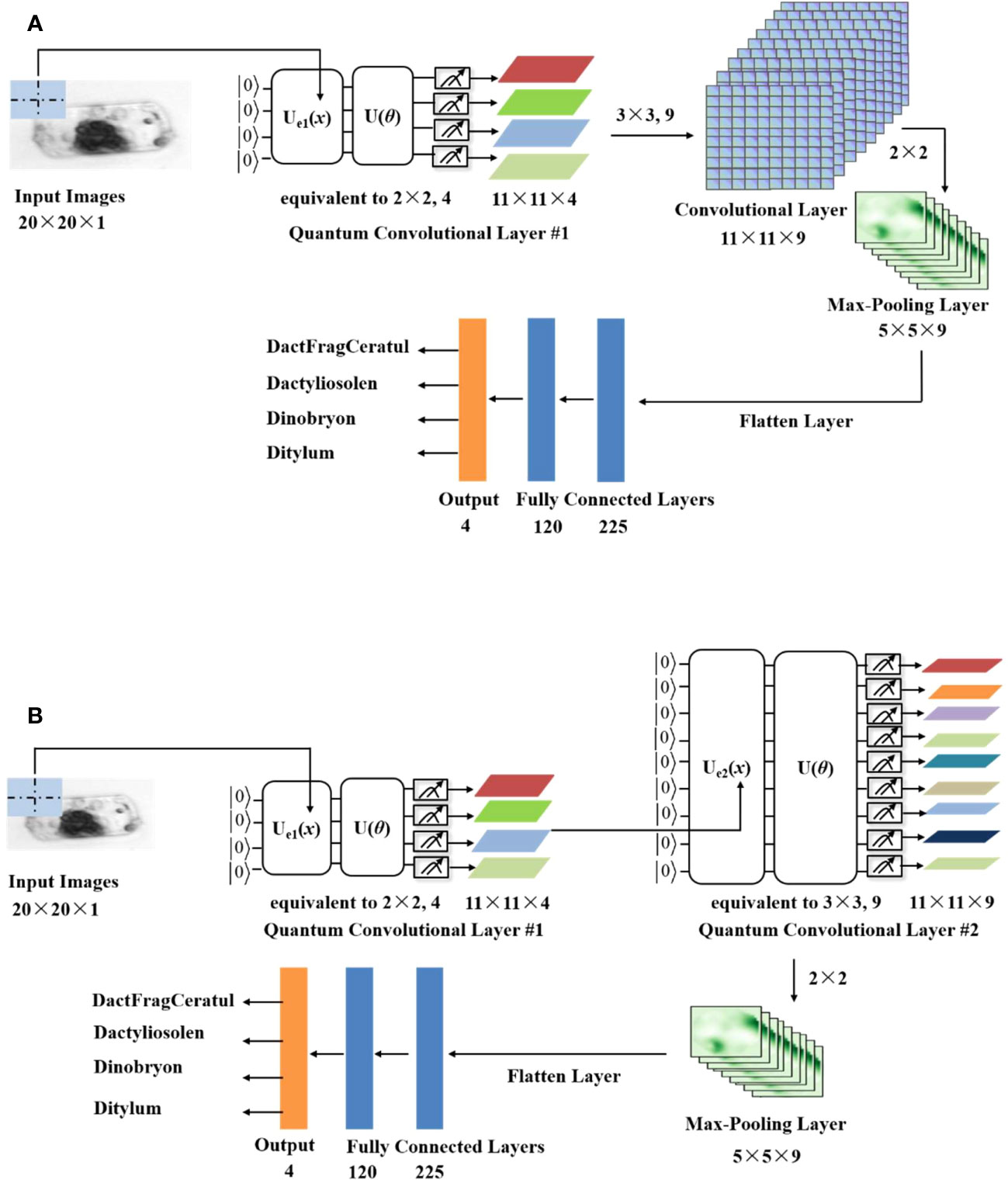
Figure 2 Architecture of the QCCNN with (A) one quantum and one classical convolutional layer (named QCCNN-1) and (B) two quantum convolutional layers (named QCCNN-2).

The models in Figure 2A and Figure 2B are named QCCNN-1 and QCCNN-2, respectively. Below, we delve into the details of the two architectures.

3.1.1 Quantum convolutional layer

The architecture of the quantum convolution layer #1 and quantum convolution layer #2 used in Figure 2 is illustrated in Figures 3A, B respectively. They consist of similar components as QNN, including the encoding circuit, ansatz circuit and quantum measurement.

FIGURE 3

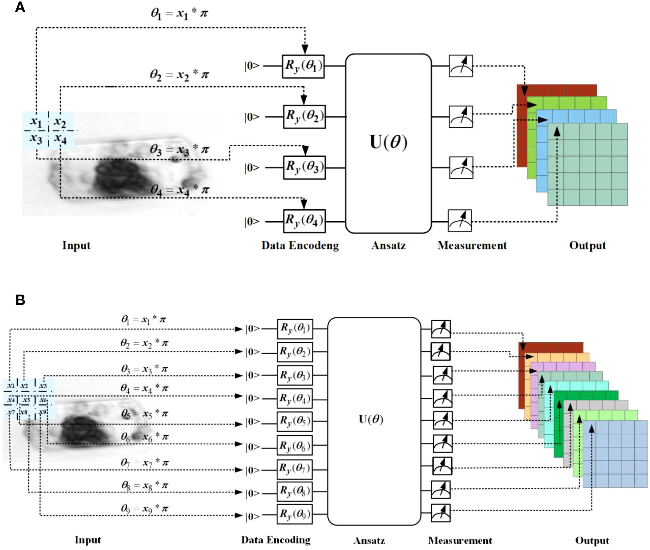
Figure 3 Architecture of the quantum convolutional layer #1 (A) and #2 (B) used in Figure 2.

In the quantum convolution layer #1, the filter window size is set to 2×2, and the four elements are embedded using four qubits through four R_y(θ) gates; while in the quantum convolution layer #2, the filter window size is set to 3×3, and the nine elements are embedded using nine qubits through nine R_y(θ) rotation gates. The ansatz is implemented using two typical hardware-efficient circuits, as shown in Figure 4. Figure 4A depicts the all-to-all configuration of two-qubit gates, which has the larger expressibility and entangling capability but the higher circuit complexity, while Figure 4B depicts the circuit-block configuration of two-qubit gates, which has the smaller expressibility and entangling capability but the lower circuit complexity (Sim et al., 2019). The expressibility and entangling capability of the ansatz can be increased by stacking the circuit as multi layers.

FIGURE 4

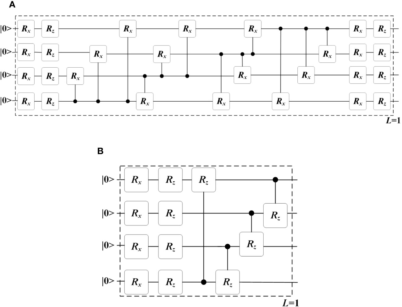
Figure 4 Two typical ansatz circuits with (A) all-to-all configuration and (B) circuit-block configuration of two-qubit gates. These circuits are used as a single layer, i.e. L = 1. Multiple layers can be stacked to increase the expressibility and entangling capability of the circuit.

Expressibility and entangling capability are two key characteristics that describe the representative capability of a PQC in the exponentially large Hilbert space (Sim et al., 2019). It’s important to note that the Hilbert space serves as the feature space of QCCNN, which means that the difference in the representative capability of the ansatz circuit can significantly affect the performance of QCCNN. However, the specific impact of this difference remains ambiguous. In the experiment section, we explore this impact in more detail.

For the quantum measurement in Figure 3, the four (nine) qubits are measured individually using the σ_z operator. The resulting probabilities of each qubit collapsing to state $|0\rangle$ are then used as four (nine) feature channels for the next layer. It’s worth noting that the quantum convolutional layer does not have an activation function, and the nonlinearity arises from the process of data encoding and quantum measurement. This is a significant difference between QNN and classical models.

3.1.2 Classical operations

The classical operations of QCCNN include classical convolutional layers, pooling layers, and fully connected layers, which follow the typical operations of CNN. Specifically, in the convolutional layers, a window size of 3×3 is used, and the activation function is the ReLu function. A Max Pooling layer is employed to reduce the number of trainable parameters. Finally, at the end of QCCNN, two fully connected layers are used to connect the convolutional and output layer.

3.2 Quantum residual network

Similar to the method used to design QCCNN, QCResNet can be constructed based on the template ResNet presented in the supplementary material (Supplementary Figure 2). Figure 5 illustrates two possible architectures for QCResNet. In Figure 5A, the QCResNet consists of one quantum residual unit and one classical residual unit, while Figure 5B has two quantum residual units. The two models are named QCResNet-1 and QCResNet-2, respectively.

FIGURE 5

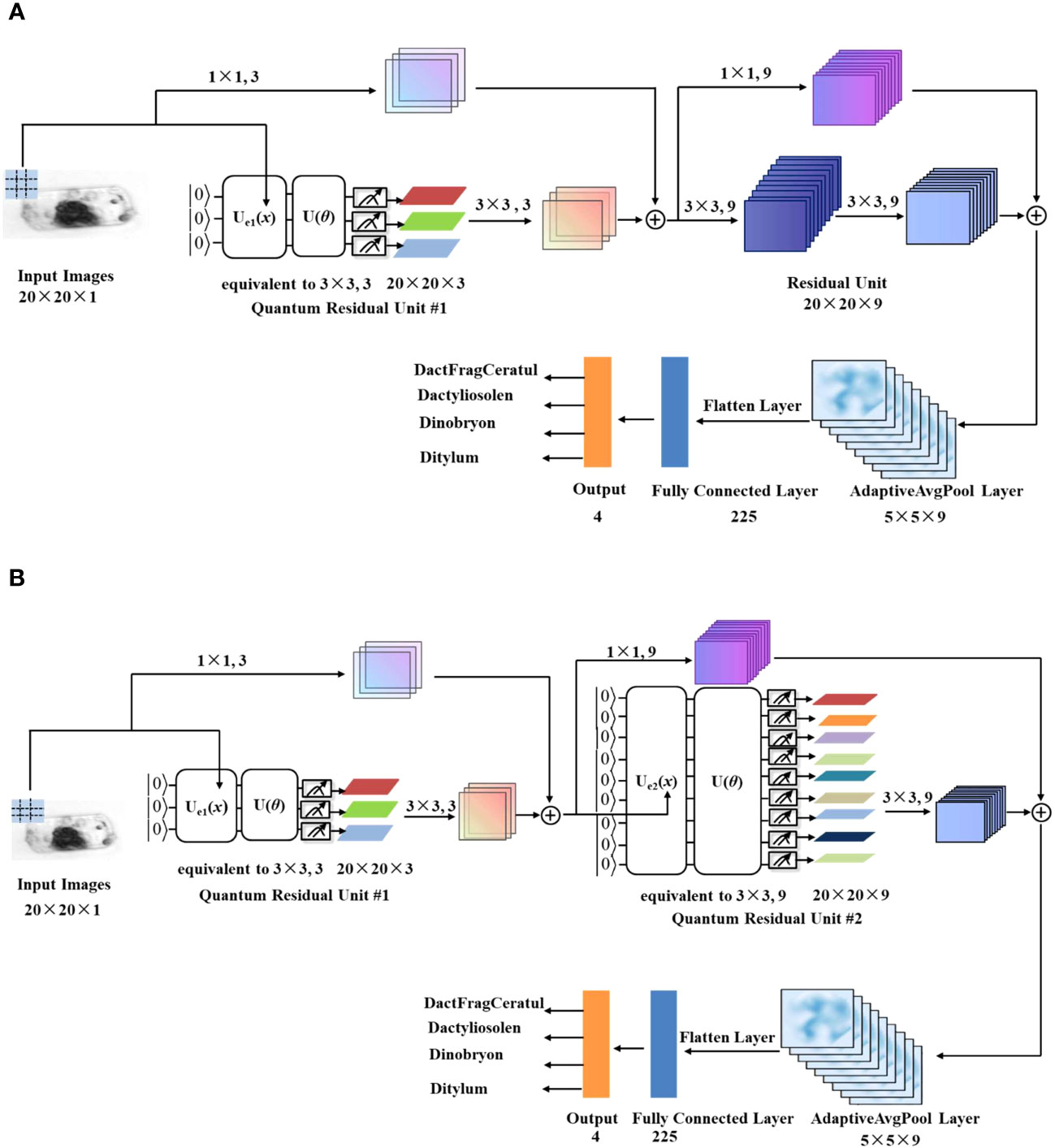
Figure 5 Architecture of the QCResNet with (A) one quantum residual unit (named QCResNet-1) and (B) two quantum residual units (named QCResNet-2).

As shown in Figure 5, both quantum residual unit #1 and quantum residual unit #2 utilize one quantum convolutional layer. It is worth noting that the quantum convolutional layer in quantum residual unit #1 uses a filter window size of 3×3, but outputs three feature channels, which differs from the one shown in Figure 3B. The architecture of the quantum convolutional layer used in quantum residual unit #1is presented in the supplementary material (Supplementary Figure 3). On the other hand, the quantum convolutional layer used in quantum residual unit #2 is identical to the one shown in Figure 3B.

4 Datasets and networks

The image dataset of phytoplankton used in this work was obtained by analyzing water from Woods Hole Harbor using a custom-built imaging-in-flow cytometer (Sosik and Olson, 2007). Sampling was conducted between late fall and early spring in 2004 and 2005. The dataset consists of 6600 images that were visually inspected and manually identified, with an even distribution across 22 categories, resulting in 300 images per category. Example images of the 22 categories are shown in Figure 6. All images were randomly divided into training set and test set, with each set containing 150 images for each category. This results in a balanced distribution of images across the categories.

FIGURE 6

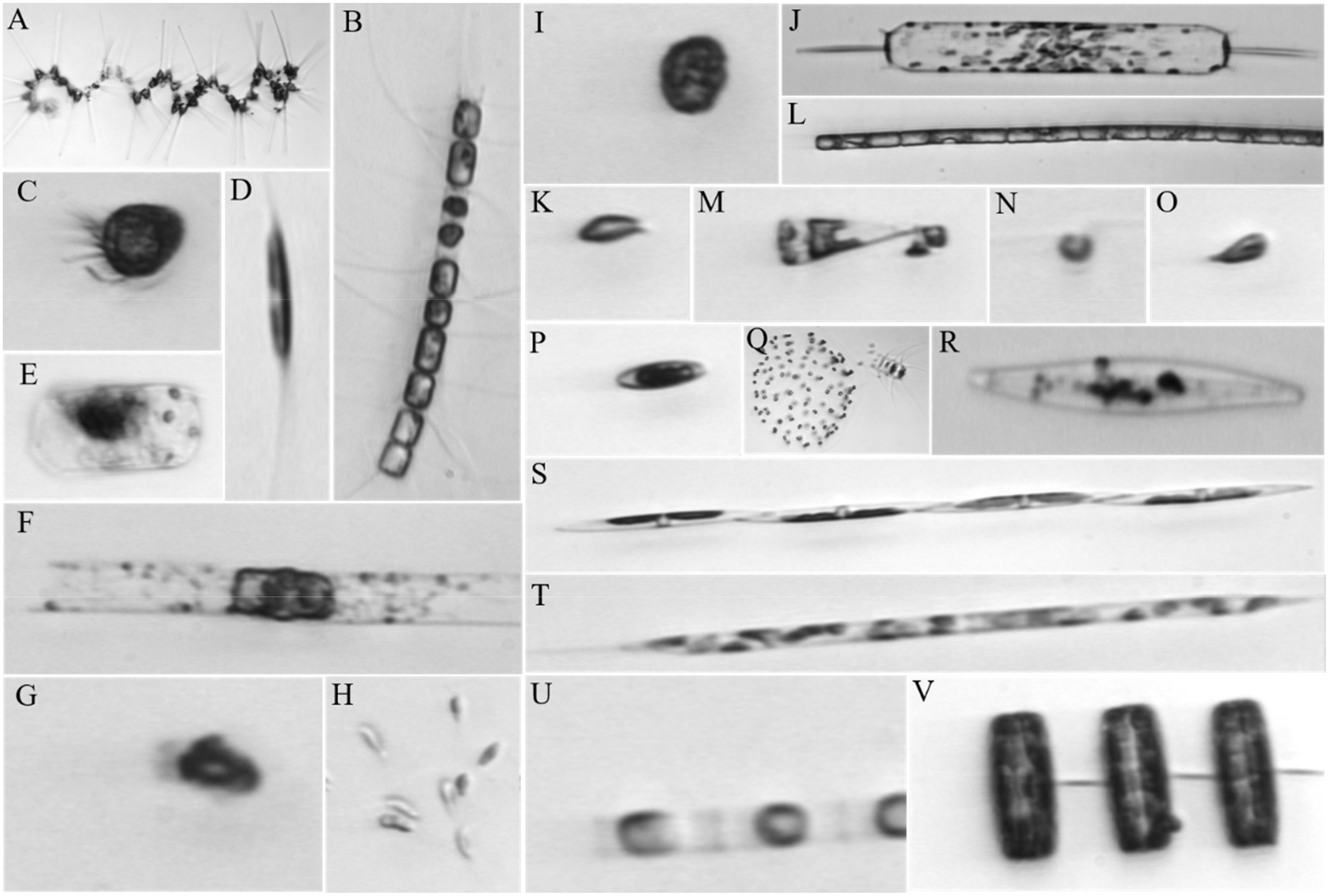
Figure 6 Example images of the 22 categories of phytoplankton: (A), Asterionellopsis; (B), Chaetoceros; (C), Ciliate; (D), Cylindrotheca; (E), DactFragCeratul; (F), Dactyliosolen; (G), Detritus; (H), Dinobryon; (I), Dinoflagellate; (J), Ditylum; (K), Euglena; (L), Guinardia; (M), Licmophora; (N), Nanoflagellate; (O), other cells< 20μm; (P), Pennate; (Q), Phaeocystis; (R), Pleurosigma; (S), Pseudonitzschia; (T), Rhizosolenia; (U), Skeletonema; (V), Thalassiosira.

In the experiment, the QCCNN and QCResNet were simulated on the classical computer, which required significant computational resources. As a result, it was not practical to train our quantum models using the full dataset of 6600 images. To address this issue, we compiled a sub-dataset consisting of 1200 images across four categories of phytoplankton, which are DactFragCeratul, Dactyliosolen, Dinobryon and Ditylum. In addition, to make the images accessible to the QCCNN and QCResNet models, all images are resized to 20×20 pixels. It is important to note that these limitations are only due to the difficulty of simulating the quantum circuit with a large number of qubits on the classical computer. The dataset used in the experiments is available on GitHub (Shi, 2023).

In the experiment, six neural networks are evaluated using the phytoplankton dataset. These networks include the template CNN (Supplementary Figure 1), template ResNet (Supplementary Figure 2), QCCNN-1 and QCCNN-2 (Figure 2), QCResNet-1 and QCResNet-2 (Figure 5). The specific architectures of these models are discussed in Section 3. A detailed comparison of their parameters is presented in the Supplementary Material (Section 3). In general, the quantum convolutional layer uses fewer parameters than the classical models, resulting in the faster convergence of the quantum models, as demonstrated in the following experiments.

In this work, the quantum and classical neural networks are implemented using the PennyLane software (Bergholm et al., 2018) and Pytorch framework, respectively. PyTorch-compatible quantum nodes in PennyLane are used to construct the hybrid quantum-classical neural networks. The loss function used is the cross-entropy function, as shown in Eq. (5). The parameters in the quantum and classical layers are trained together and updated based on the SGD method. The number of shots used in the quantum measurement is set to 1500, as discussed in the Supplementary Material (Section 4). The six neural networks have learning rates ranging from 0.05 to 0.1, with a batch size of 15 and trained for 50 epochs each.

5 Experimental results and discussions

5.1 Training loss and classification accuracy

To compare the performance of classical and quantum models, we first analyze the models’ training loss and classification accuracy. Figure 7 displays the curves of the training loss and test classification accuracy of the template CNN and QCCNN models. It is clear from the curves that the QCCNN model converges much faster than the CNN model. Furthermore, the classification accuracy of QCCNN-1 is 93.67%, which is almost the same as that of CNN. However, the accuracy fluctuation of QCCNN is much smaller, indicating that QCCNN has better generalization. The stronger performance of QCCNN can be attributed to the unique feature space of QCCNN, that is, the exponentially large Hilbert space created by the quantum circuit. This quantum feature space enables QCCNN to capture more abstract information from the data and generalize better. As the number of qubits and depth of quantum circuit increase, the quantum feature space will become completely intractable for classical computers, leading to a quantum advantage for QCCNN.

FIGURE 7

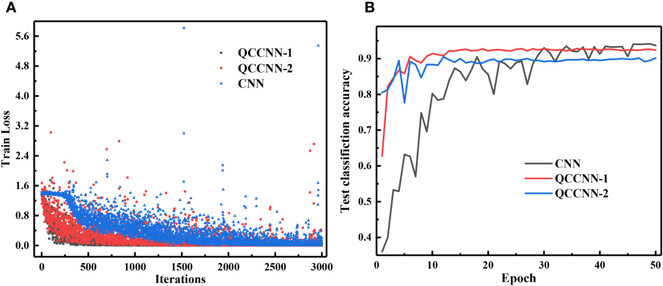
Figure 7 Curves of the training loss (A) and test classification accuracy (B) of CNN and QCCNN for phytoplankton classification.

In addition, it’s interesting to note that the accuracy of QCCNN-1 is higher than that of QCCNN-2. The experiments show that adding more quantum convolutional layers to QCCNN does not necessarily improve the model’s performance. This is likely because more quantum convolutional layers significantly increase the feature space, making it more difficult to train the model. Therefore, the number and position of quantum convolutional layers used in QCCNN should be optimized for the specific learning tasks. Similar results have also been observed in the quantum-inspired CNN (Shi et al., 2022).

The curves for the training loss and test classification accuracy of the template ResNet and QCResNet models are shown in Figure 8. Similar to the findings for QCCNN, QCResNet exhibits similar features. QCResNet converges faster than ResNet; the classification accuracy of QCResNet-1 is 94.5%, which is higher than ResNet’s 91.5%; QCResNet shows much smaller fluctuations in accuracy compared to ResNet. The larger fluctuations in the training loss and accuracy curves of ResNet, compared to CNN, can be reduced by increasing the depth of the networks. Additionally, the performance of QCResNet-1 is better than that of QCResNet-2, indicating that the number and position of quantum convolutional layers used in QCResNet should be optimized for the specific learning tasks, as it is for QCCNN.

FIGURE 8

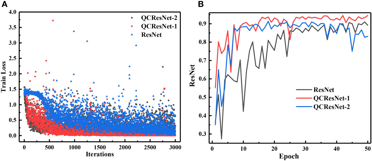
Figure 8 Curves of the training loss (A) and test classification accuracy (B) of ResNet and QCResNet for phytoplankton classification.

5.2 Confusion matrix and other evaluation metric

In order to conduct a more comprehensive evaluation of the model’s classification performance, we compute the confusion matrices of the results obtained by the six neural networks, as shown in Figure 9. A confusion matrix is an N × N matrix, where N represents the number of target categories. It summarizes the correct and incorrect predictions generated by the models on the multiple-class classification task.

FIGURE 9

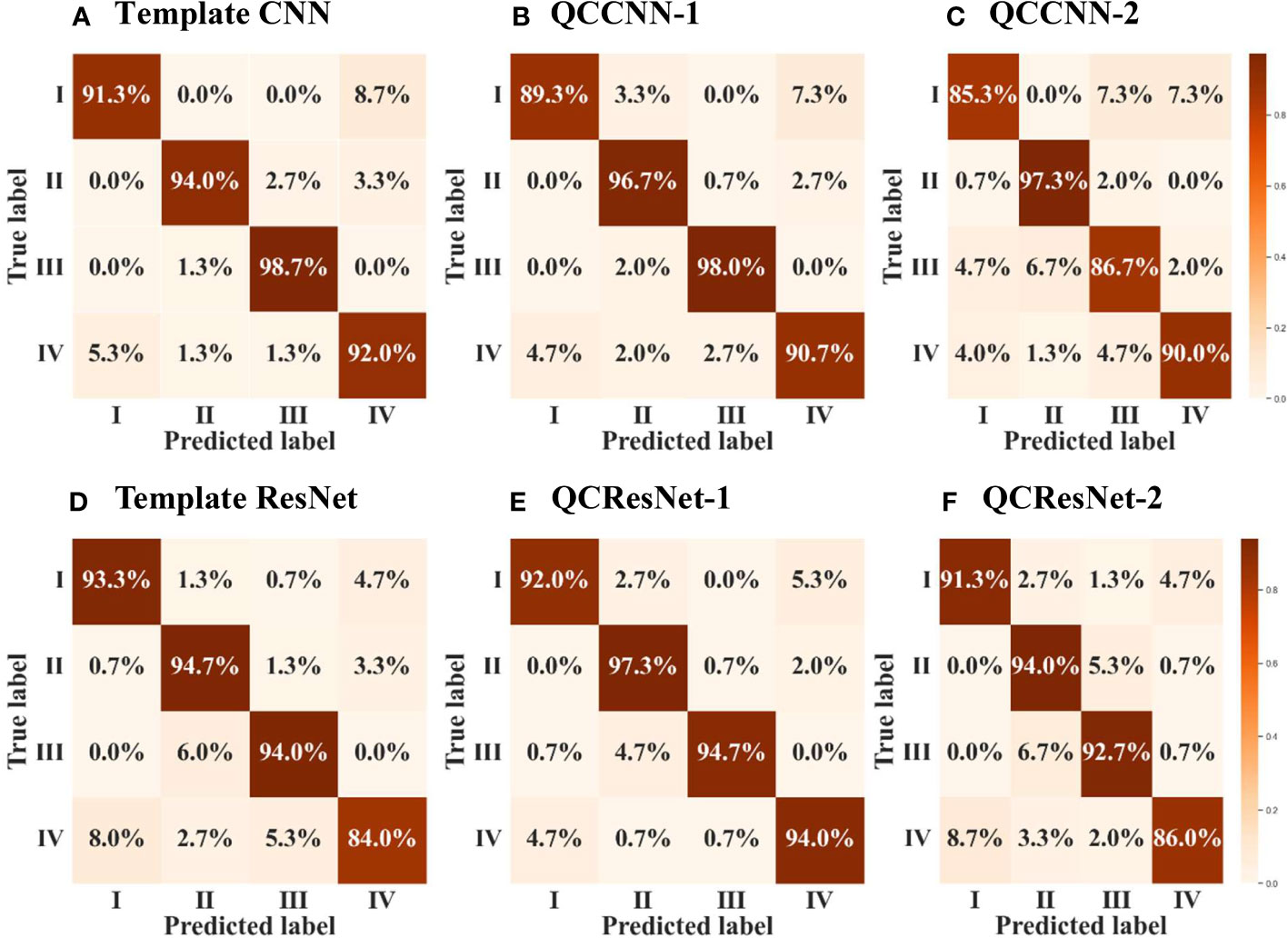
Figure 9 Confusion matrix of the results obtained by the six neural networks, namely (A) template CNN, (B) QCCNN-1, (C) QCCNN-2, (D) template ResNet, (E) QCResNet-1 and (F) QCResNet-2. The classes I, II, III and IV represent DactFragCeratul, Dactyliosolen, Dinobryon and Detritus, respectively.

Furthermore, based on the confusion matrices, we calculate additional evaluation metrics, in addition to classification accuracy, to analyze the generalization ability of the six neural networks. These metrics include precision, recall, F1-score, specificity, false positive rate (FPR), false discovery rate (FDR) and false negative rate (FNR). The definitions of these metrics can be found in the Supplementary Material (Section 5). Table 1 presents the results, where the metrics are computed as the arithmetic mean of the metric values for each class, namely the macro metric, as illustrated in the supplementary.

TABLE 1

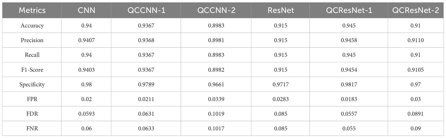
Table 1 Results of the eight evaluation metrics for the six neural networks.

Now we can analyze the performance of the six neural networks in greater detail, based on the confusion matrix in Figure 9 and the evaluation metrics presented in Table 1. Firstly, QCResNet-1 outperforms the other models in all evaluation metrics, indicating that the use of a residual architecture effectively enhances the performance of QCCNN. In particular, when compared to ResNet, QCResNet-1 exhibits significantly stronger performance on type IV phytoplankton (i.e. Detritus), as shown in Figure 9. However, QCResNet-1 performs poorly on type III phytoplankton (i.e. Dinobryon) when compared to the CNN and QCCNN-1 models. In general, QCResNet-1, QCCNN-1 and CNN models achieve comparable performance in terms of evaluation metrics; however, their classification outcomes differ significantly across the four phytoplankton categories.

Secondly, the QCCNN-2, QCResNet-2 and ResNet models exhibit poor performance, which is consistent with the results shown in Figures 7 , 8. As per Figure 9, the primary weakness of QCCNN-2 is its poor performance on type III phytoplankton, with a prediction accuracy that is approximately 10 percentage points lower. On the other hand, QCResNet-2 performs poorly on type IV phytoplankton. In future work, it would be interesting to compare the performance of these models on other datasets and learning tasks.

5.3 Influence of ansatz circuit for QCCNN

The quantum convolutional layer is a crucial element of both QCCNN and QCResNet. Its primary function is to utilize the ansatz circuit, i.e. a PQC, as a filer to perform the forward transformation in CNN. Therefore, the features of the ansatz circuit have a significant impact on the performance of QCCNN and QCResNet. Analyzing this relationship can help improve the performance of QNN models.

The ansatz circuit can be quantitatively characterized by its expressibility and entangling capability (Sim et al., 2019). Expressibility refers to the ability of a circuit to generate states that are highly representative of the Hilbert space. One way to calculate expressibility is by comparing the distribution of states generated by sampling the PQC’s parameters to the uniform distribution of states in the Haar-random state ensemble. On the other hand, entangling capability describes the correlation between multiple qubits, that is, the inherent correlation within the quantum state. The entangling capability of an ansatz circuit can be quantified using the entanglement measures, such as the Meyer-Wallach measure. Generating highly entangled states with low-depth circuits can provide significant advantages for QNN, such as the ability to capture non-trivial correlations in quantum data.

There should be a relationship between the expressibility and entangling capability of the ansatz circuit and the performance of the corresponding QNNs. Below, we use QCCNN-1 as the basic model to exploit this dependence. Note that in the experiments discussed above, QCCNN-1 uses the circuit shown in Figure 4A as its ansatz. As mentioned in Section 3.1.1, Figure 4A circuit has higher expressibility and entangling capability, while Figure 4B circuit is lower but can be stacked to increase its expressibility and entangling capability. By replacing the ansatz of QCCNN-1 with multiple layers of Figure 4B circuit, we obtain five versions of QCCNN-1.

The classification accuracy of the five versions of QCCNN-1 is shown in Figure 10. The figure shows that QCCNN-1 using Figure 4A circuit as the ansatz achieves higher accuracy compared to that using Figure 4B. This suggests that higher expressibility and entangling capability of the ansatz circuit can indeed result in better performance of the QCCNN model.

FIGURE 10

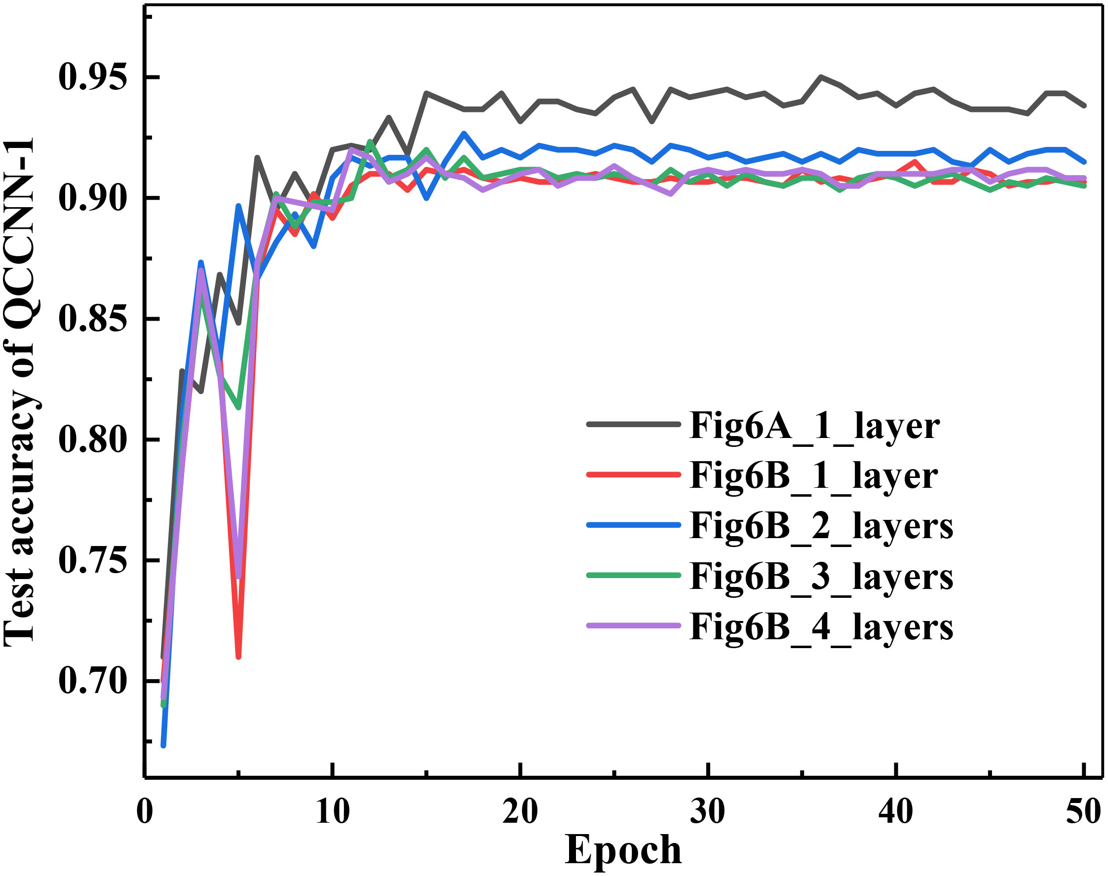
Figure 10 Classification accuracy of the five versions of QCCNN-1, which utilize the circuit of Figure 4A and 1, 2, 3 and 4 layers of Figure 4B as the ansatz.

However, for QCCNN-1 using multi-layers of Figure 4B as the ansatz, the accuracy does not always increase with the number of layers. Specifically, the accuracy of QCCNN-1 with 2 layers is the highest, while those with 1, 3 and 4 layers are close. Note that the circuit using 4 layers of Figure 4B achieves similar expressibility and entangling capability as that of Figure 4A, as presented in (Sim et al., 2019). Therefore, this suggests that in addition to the properties of expressibility and entangling capability, there are other influential factors on the models’ performance.

One such factor is the number of trainable parameters. When the number of layers is increased, the expressibility and entangling capability increase, but so does the number of trainable parameters. More parameters make the model more difficult to train, which can decrease its generalization and offset the positive effect of increasing the expressibility and entangling capability. Another factor is the topological structure of the ansatz circuit. A quantitative method for characterizing the architecture of PQC and its correlation to the performance of the corresponding QCCNN need to be exploited in detail. We leave this for future work.

6 Conclusion

In this work, we develop several hybrid quantum-classical convolutional and residual neural networks and demonstrate their efficiency for phytoplankton classification. The QCCNN and QCResNet models are constructed by incorporating quantum-enhanced forward transformations into classical CNN and ResNet models. These hybrid architectures strike a good balance between the limited functionality of current NISQ devices and the large-size images of phytoplankton.

QCResNet outperforms classical models in terms of prediction performance, while QCCNN performs comparably to its classical counterparts. More remarkably, both QCCNN and QCResNet exhibit much faster convergence and more stable classification accuracy curves, with less fluctuation. We also find that the performance of QCCNN and QCResNet depends on several factors, including the expressibility, entangling capability and topological structure of the ansatz circuit, as well as the number of training parameters. By considering all these factors, the model’s performance can be improved. Our QCCNN and QCResNet models are versatile and can be easily expanded for other image classification tasks.

In the future, we plan to optimize the architecture of QCCNN and QCResNet from both quantum and classical perspectives. This includes optimizing the structure of quantum convolutional layer and the template CNN and ResNet architecture. Additionally, due to computational resources limitations, in this work we construct a mini model of QCNN and evaluate its performance using a relatively small dataset. In the future, it will be necessary to demonstrate the scalability of our models and find practical and advantageous applications in more marine science tasks.

Data availability statement

The raw data supporting the conclusions of this article will be made available by the authors, without undue reservation.

Author contributions

SS and ZW developed the algorithms and wrote the first draft. SS, RS, YL and JL wrote the codes and carried out the numerical experiments. YG, GZ and ZW planned and designed the project. All authors discussed the results and reviewed the manuscript. All authors contributed to the article and approved the submitted version

Funding

The present work is supported by the Natural Science Foundation of Shandong Province of China (ZR2021ZD19) and the National Natural Science Foundation of China (12005212).

Acknowledgments

We are grateful to the support of computational resources from the Marine Big Data Center of Institute for Advanced Ocean Study of Ocean University of China.

Conflict of interest

The authors declare that the research was conducted in the absence of any commercial or financial relationships that could be construed as a potential conflict of interest.

Publisher’s note

All claims expressed in this article are solely those of the authors and do not necessarily represent those of their affiliated organizations, or those of the publisher, the editors and the reviewers. Any product that may be evaluated in this article, or claim that may be made by its manufacturer, is not guaranteed or endorsed by the publisher.

Supplementary material

The Supplementary Material for this article can be found online at: https://www.frontiersin.org/articles/10.3389/fmars.2023.1158548/full#supplementary-material

References

Arute F., Arya K., Babbush R., Bacon D., Bardin J. C., Barends R., et al. (2019). Quantum supremacy using a programmable superconducting processor. Nature 574 (7779), 505–510. doi: 10.1038/s41586-019-1666-5

PubMed Abstract | CrossRef Full Text | Google Scholar

Baek S. S., Jung E. Y., Pyo J., Pachepsky Y., Son H., Cho K. H. (2022). Hierarchical deep learning model to simulate phytoplankton at phylum/class and genus levels and zooplankton at the genus level. Water Res. 218, 118494. doi: 10.1016/j.watres.2022.118494

PubMed Abstract | CrossRef Full Text | Google Scholar

Barton A. D., Dutkiewicz S., Flierl G., Bragg J., Follows M. J. (2010). Patterns of diversity in marine phytoplankton. Science 327 (5972), 1509–1511. doi: 10.1126/science.1184961

PubMed Abstract | CrossRef Full Text | Google Scholar

Benedetti M., Lloyd E., Sack S., Fiorentini M. (2019). Parameterized quantum circuits as machine learning models. Quantum Sci. Technol. 4 (4), 043001. doi: 10.1088/2058-9565/ab4eb5

CrossRef Full Text | Google Scholar

Bergholm V., Izaac J., Schuld M., Gogolin C., Ahmed S., Ajith V., et al. (2018). Pennylane: Automatic differentiation of hybrid quantum-classical computations. arXiv:1811.04968. doi: 10.48550/arXiv.1811.04968

CrossRef Full Text | Google Scholar

Bharti K., Cervera-Lierta A., Kyaw T. H., Haug T., Alperin-Lea S., Anand A., et al. (2022). Noisy intermediate-scale quantum algorithms. Rev. Modern Phys. 94 (1), 15004. doi: 10.1103/RevModPhys.94.015004

CrossRef Full Text | Google Scholar

Biamonte J., Wittek P., Pancotti N., Rebentrost P., Wiebe N., Lloyd S. (2017). Quantum machine learning. Nature 549, 195. doi: 10.1038/nature23474

CrossRef Full Text | Google Scholar

Chen S. Y. C., Wei T. C., Zhang C., Yu H., Yoo S. (2022). Quantum convolutional neural networks for high energy physics data analysis. Phys. Rev. Res. 4 (1), 13231. doi: 10.1103/PhysRevResearch.4.013231

CrossRef Full Text | Google Scholar

Cong I., Choi S., Lukin M. D. (2019). Quantum convolutional neural networks. Nat. Physics. 15 (12), 1273–1278. doi: 10.1038/s41567-019-0648-8

CrossRef Full Text | Google Scholar

Cui J., Wei B., Wang C., Yu Z., Zheng H., Zheng B., et al. (2018). “Texture and shape information fusion of convolutional neural network for plankton image classification,” in 2018 OCEANS - MTS/IEEE Kobe Techno-Oceans (OTO), Kobe, Japan. 1–5. doi: 10.1109/OCEANSKOBE.2018.8559156

CrossRef Full Text | Google Scholar

Dagtekin O., Dethlefs N. (2022). “Modelling phytoplankton behaviour in the north and irish sea with transformer networks,” in Proceedings of the Northern Lights Deep Learning Workshop, Vol. 3. doi: 10.7557/18.6229

CrossRef Full Text | Google Scholar

Dai J., Yu Z., Zheng H., Zheng B., Wang N. (2017). “A hybrid convolutional neural network for plankton classification,” in Computer Vision–ACCV 2016 Workshops: ACCV 2016 International Workshops, Vol. 102-114. doi: 10.1007/978-3-319-54526-4_8

CrossRef Full Text | Google Scholar

Deng D. (2021). Quantum enhanced convolutional neural networks for NISQ computers. Sci. China Phys. Mech. Astron. 64 (10), 100331. doi: 10.1007/s11433-021-1758-0

CrossRef Full Text | Google Scholar

Dosovitskiy A., Beyer L., Kolesnikov A., Weissenborn D., Zhai X., Unterthiner T., et al. (2020). An image is worth 16x16 words: Transformers for image recognition at scale. arXiv:2010.11929.. doi: 10.48550/arXiv.2010.11929

CrossRef Full Text | Google Scholar

Faillettaz R., Picheral M., Luo J. Y., Guigand C., Cowen R. K., Irisson J. O. (2016). Imperfect automatic image classification successfully describes plankton distribution patterns. Methods Oceanogr. 15, 60–77. doi: 10.1016/j.mio.2016.04.003

CrossRef Full Text | Google Scholar

Fuchs R., Thyssen M., Creach V., Dugenne M., Izard L., Latimier M., et al. (2022). Automatic recognition of flow cytometric phytoplankton functional groups using convolutional neural networks. Limnol. Oceanogr. Methods. 20 (7), 387–399. doi: 10.1002/lom3.10493

CrossRef Full Text | Google Scholar

Gittings J. A., Raitsos D. E., Krokos G., Hoteit I. (2018). Impacts of warming on phytoplankton abundance and phenology in a typical tropical marine ecosystem. Sci. Rep. 8 (1), 1–12. doi: 10.1038/s41598-018-20560-5

CrossRef Full Text | Google Scholar

Glüge S., Pomati F., Albert C., Kauf P., Ott T. (2014). “The challange of clustering flow cytometry data from phytoplankton in lakes,” in Nonlinear dynamics of electronic systems. NDES 2014. Communications in computer and information science, vol. 438 . Eds. Mladenov V. M., Ivanov P. C. (Cham: Springer). doi: 10.1007/978-3-319-08672-9_45

CrossRef Full Text | Google Scholar

Havlíček V., Córcoles A. D., Temme K., Harrow A. W., Kandala A., Chow J. M., et al. (2017). Supervised learning with quantum-enhanced feature spaces. Nature 567, 209. doi: 10.1038/s41586-019-0980-2

CrossRef Full Text | Google Scholar

Houssein E. H., Abohashima Z., Elhoseny M., Mohamed W. M. (2022). Hybrid quantum-classical convolutional neural network model for COVID-19 prediction using chest X-ray images. J. Comput. Design Eng. 9 (2), 343–363. doi: 10.1093/jcde/qwac003

CrossRef Full Text | Google Scholar

Hu Q., Davis C. (2005). Automatic plankton image recognition with co-occurrence matrices and support vector machine. Mar. Ecol. Prog. Series. 295, 21–31. doi: 10.3354/meps295021

CrossRef Full Text | Google Scholar

Hur T., Kim L., Park D. K. (2022). Quantum convolutional neural network for classical data classification. Quantum Mach. Intell. 4 (1), 1–18. doi: 10.1007/s42484-021-00061-x

CrossRef Full Text | Google Scholar

Jeswal S. K., Chakraverty S. (2019). Recent developments and applications in quantum neural network: a review. Arch. Comput. Methods Eng. 26 (4), 793–807. doi: 10.1007/s11831-018-9269-0

CrossRef Full Text | Google Scholar

Kwak Y., Yun W. J., Jung S., Kim J. (2021). “Quantum neural networks: Concepts, applications, and challenges,” in 2021 Twelfth International Conference on Ubiquitous and Future Networks (ICUFN). 413–416. doi: 10.1109/ICUFN49451.2021.9528698

CrossRef Full Text | Google Scholar

Kyathanahally S. P., Hardeman T., Reyes M., Merz E., Bulas T., Brun P., et al. (2022). Ensembles of data-efficient vision transformers as a new paradigm for automated classification in ecology. Sci. Rep. 12 (1), 18590. doi: 10.1038/s41598-022-21910-0

CrossRef Full Text | Google Scholar

Li G., Zhao X., Wang X. (2022). Quantum self-attention neural networks for text classification. arXiv:2205.05625. doi: 10.48550/arXiv.2205.05625

CrossRef Full Text | Google Scholar

Liu J., Lim K. H., Wood K. L., Huang W., Guo C., Huang H. L. (2021). Hybrid quantum-classical convolutional neural networks. Sci. China Phys. Mech. Astron. 64 (9), 1–8. doi: 10.1007/s11433-021-1734-3

CrossRef Full Text | Google Scholar

Madsen L. S., Laudenbach F., Askarani M. F., Rortais F., Vincent T., Bulmer J. F. F., et al. (2022). Quantum computational advantage with a programmable photonic processor. Nature 606, 75–81. doi: 10.1038/s41586-022-04725-x

CrossRef Full Text | Google Scholar

Mattei F., Franceschini S., Scardi M. (2018). A depth-resolved artificial neural network model of marine phytoplankton primary production. Ecol. Model. 382, 51–62. doi: 10.1016/j.ecolmodel.2018.05.003

CrossRef Full Text | Google Scholar

Mattei F., Scardi M. (2020). Embedding ecological knowledge into artificial neural network training: A marine phytoplankton primary production model case study. Ecol. Model. 421, 108985. doi: 10.1016/j.ecolmodel.2020.108985

CrossRef Full Text | Google Scholar

Oh S., Choi J., Kim J. (2020). “A tutorial on quantum convolutional neural networks (QCNN),” in 2020 International Conference on Information and Communication Technology Convergence (ICTC). 236–239. doi: 10.1109/IDAACS53288.2021.9661011

CrossRef Full Text | Google Scholar

Owen B. M., Hallett C. S., Cosgrove J. J., Tweedley J. R., Moheimani N. R. (2022). Reporting of methods for automated devices: A systematic review and recommendation for studies using FlowCam for phytoplankton. Limnol. Oceanogr. Methods 20 (7), 400–427. doi: 10.1002/lom3.10496

CrossRef Full Text | Google Scholar

Pastore V. P., Zimmerman T. G., Biswas S. K., Bianco S. (2020). Annotation-free learning of plankton for classification and anomaly detection. Sci. Rep. 10 (1), 1–15. doi: 10.1038/s41598-020-68662-3

CrossRef Full Text | Google Scholar

Preskill J. (2018). Quantum computing in the NISQ era and beyond. Quantum 2, 79. doi: 10.22331/q-2018-08-06-79

CrossRef Full Text | Google Scholar

Schuld M., Killoran N. (2019). Quantum machine learning in feature Hilbert spaces. Phys. Rev. Lett. 122 (4), 40504. doi: 10.1103/PhysRevLett.122.040504

CrossRef Full Text | Google Scholar

Shao R., Bi X. J., Chen Z. (2022). A novel hybrid transformer-CNN architecture for environmental microorganism classification. PloS One 17 (11), e0277557. doi: 10.1371/journal.pone.0277557

CrossRef Full Text | Google Scholar

Shi S. (2023) QCCNN-dataSet. Available at: https://github.com/sunyyds2020/QCCNN-DataSet.git.

Google Scholar

Shi S., Wang Z., Cui G., Wang S., Shang R., Li W., et al. (2022). Quantum-inspired complex convolutional neural networks. Appl. Intell. 52, 17912–17921. doi: 10.1007/s10489-022-03525-0

CrossRef Full Text | Google Scholar

Shi S., Wang Z., Li J., Li Y., Shang R., Zheng H., et al. (2023). A natural NISQ model of quantum self-attention mechanism. arXiv:2305.15680. doi: 10.48550/arXiv.2305.15680

CrossRef Full Text | Google Scholar

Sim S., Johnson P. D., Aspuru-Guzik A. (2019). Expressibility and entangling capability of parameterized quantum circuits for hybrid quantum-classical algorithms. Adv. Quantum Technol. 2 (12), 1900070. doi: 10.1002/qute.201900070

CrossRef Full Text | Google Scholar

Sosik H. M., Olson R. J. (2007). Automated taxonomic classification of phytoplankton sampled with imaging-in-flow cytometry. Limnol. Oceanogr. Methods 5 (6), 204–216. doi: 10.4319/lom.2007.5.204

CrossRef Full Text | Google Scholar

Verikas A., Gelzinis A., Bacauskiene M., Olenina I., Vaiciukynas E. (2014). An integrated approach to analysis of phytoplankton images. IEEE J. Oceanic Eng. 40 (2), 315–326. doi: 10.1109/JOE.2014.2317955

CrossRef Full Text | Google Scholar

Wang C., Zheng X., Guo C., Yu Z., Yu J., Zheng H., et al. (2018). “Transferred parallel convolutional neural network for large imbalanced plankton database classification,” in 2018 OCEANS - MTS/IEEE Kobe Techno-Oceans (OTO). 1–5. doi: 10.1109/OCEANSKOBE.2018.8558836

CrossRef Full Text | Google Scholar

Wierichs D., Izaac J., Wang C., Lin C. Y. Y. (2022). General parameter-shift rules for quantum gradients. Quantum 6, 677. doi: 10.22331/q-2022-03-30-677

CrossRef Full Text | Google Scholar

Zhao R. X., Shi J., Zhang S., Li X. L. (2022). QSAN: A near-term achievable quantum self-attention network. arXiv:2207.07563. doi: 10.48550/arXiv.2207.07563

CrossRef Full Text | Google Scholar

Zheng H., Wang R., Yu Z., Wang N., Gu Z., Zheng B. (2017). Automatic plankton image classification combining multiple view features via multiple kernel learning. BMC Bioinf. 18 (16), 1–18. doi: 10.1186/s12859-017-1954-8

CrossRef Full Text | Google Scholar

Zhong H., Wang H., Deng Y., Chen M., Peng L., Qin J., et al. (2020). Quantum computational advantage using photons. Science 370, 1460–1463. doi: 10.1126/science.abe8770

CrossRef Full Text | Google Scholar