Upwelling processes driven by contributions from wind and current in the Southwest East Sea (Japan Sea)

1 Introduction

Coastal upwelling resulting from alongshore wind stress causes the offshore Ekman transport of surface waters (Huyer, 1983; Lentz and Chapman, 2004; Estrade et al., 2008; Jacox and Edwards, 2011). The occurrence of this phenomenon is primarily related to the strength and duration of the alongshore wind stress. Moreover, such upward onshore flow transports nutrient-rich water from the subsurface layer into the euphotic layer and stimulates the growth of phytoplankton and zooplankton (Lentz and Chapman, 2004; Chen et al., 2013; Shin et al., 2017). Coastal upwelling promotes the growth of certain species in unfavorable environments because of the sudden drop in water temperature (Alvarez et al., 2010). In the southwestern East Sea (Japan Sea; ES hereafter), coastal upwelling occurs with southerly winds during the summer (Seung, 1974; Lee, 1983; Lee and Na, 1985; Lee et al., 1998). From July to August, the East Asian Summer Monsoon system maintains a southerly or southwesterly wind flow that is responsible for coastal upwelling along the east coast of Korea, whereas northerly and northwesterly winds prevail in the winter (Lee, 1983; Lee and Na, 1985; Yoo and Park, 2009). Suh et al. (2001) reported that when southerly winds blow at speeds of approximately 3–5 m s⁻¹, the water temperature is generally reduced by 1–3°C and 2–7°C, respectively. Strong southerly winds of more than 6 m s⁻¹ cause an extreme drop in water temperature along the east coast of Korea, leading to upwelling in just one day (Lee et al., 1998).

However, numerous factors are related to coastal upwelling intensity. Kim and Kim (2008) suggested that wind stress, adjacent bathymetry structure, and coastline orientation are the dominant factors contributing to the occurrence of coastal upwelling based on numerical model experiments. Furthermore, Ji et al. (2019) suggested the importance of cross-shore transport caused by the alongshore current using a scale analysis of the Gampo-Ulgi (GU) (Figure 1). Even if the upwelling-favorable wind is no longer present, the persistent alongshore current maintains the surface cold water for a couple of weeks along the southern coast of Korea (Jung and Cho, 2020). Lentz and Chapman (2004) described that the vertical velocity structure of upwelling and forces governing the compensational flow of offshore surface currents could be altered by the stratification intensity represented by the Burger number.

FIGURE 1

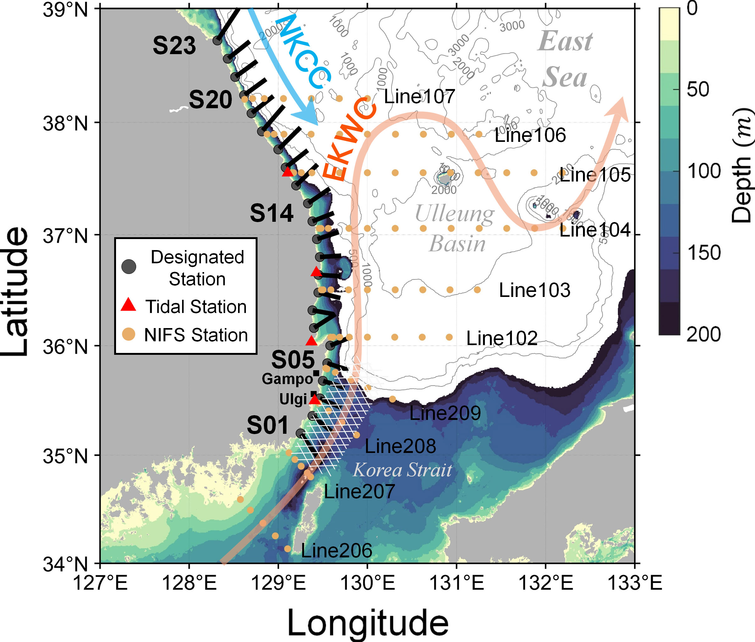
Figure 1 Study area based on topography derived from GEBCO and shown with contours. Black dots indicate designated stations, and red triangles represent observation stations (Ulsan [S03], Pohang [S07], Hupo [S10], and Mukho [S16]). Black lines show the cross-shore direction at each station. Orange dots are bimonthly repeated shipboard observation stations by the National Institute of Fisheries Science. Red and blue arrows indicate the mean flow defined as the East Korea Warm Current (EKWC) and North Korea Cold Current (NKCC), respectively. The S03 and S04 are known as Gampo-Ulgi (GU). The regions with white hash patterns off the coast of S01 through S05 are defined as the southern regions of the study area, whereas other stations are defined as the northern regions.

As shown in Figure 1, the east coast of Korea is influenced by a branch of the Kuroshio Current, the East Korea Warm Current (EKWC). The EKWC is transported through the Korea Strait and is analogous to the Western Boundary Current (WBC). The volume transport of the EKWC is approximately 1.5 Sv, which accounts for approximately 60% of the entire transport through the strait and gradually augments during the upwelling-favorable wind-blowing season (Chang et al., 2002; Kim et al., 2004). The EKWC causes current-driven upwelling; however, how the alongshore current influences the development of coastal upwelling in the southwest ES is not addressed. Therefore, this study aims to (1) estimate the impact of each geophysical factor by investigating the effect of upwelling index usage and (2) explain the results obtained by the analysis of the index in terms of dynamics.

Many indices have been used to predict upwelling events, such as the index using wind stress (Bakun, 1975). The index incorporates wind and ocean properties, such as sea surface temperature (García-Reyes et al., 2014), that relate the dynamics and structure of the cross-shelf circulation to stratification, bathymetry, and wind stress (Lentz and Chapman, 2004; Jacox and Edwards, 2011), or that characterize upwelling more completely from theory (Rossi et al., 2013) and model output (Jacox and Edwards, 2011; Jacox et al., 2018). In this study, we used an index named “Upwelling Age (UA)” (Jiang et al., 2012), which was improved by Chen et al. (2013), to understand upwelling occurrences and quantify the contribution of factors to coastal upwelling. The index is a non-dimensional number defined as the ratio of two different time scales: the wind event and the advection time scale (Jiang et al., 2012). The wind event time scale (i.e., wind duration) is a concept of how long the upwelling-favorable wind persists. In contrast, the advection time scale represents the time at which the water column is advected from the bottom layer to the surface layer. Thus, this index may be the most appropriate for analyzing different geophysical forcings for upwelling events.

To examine the upwelling processes, driven either by winds or currents, we first examined UA at 23 stations at regular latitudinal distances (approximately 16 km) along the east coast of the Korean Peninsula (Figure 1). Subsequently, the most determinant components at each station were quantitatively evaluated and compared with long-term in situ observations. The rest of this article is organized as follows: the data sources and analytical methods are described in Section 2. For the specific results, a temporal consistency comparison between UA and the water temperature measurements and geophysical contributors to UA is evaluated in Sections 3.1 and 3.2. In Section 3.3, the fraction of upwelled water masses estimated by water mass analysis is directly compared to the intensity of upwelling-favorable wind and alongshore currents. The dynamics of wind- and current-driven upwelling are discussed in Section 4, and the results discussed in Section 3 are explained in terms of physical oceanography. To examine geostrophic current-induced upwelling processes, barotropic and baroclinic conditions were considered in Sections 4.1 and 4.2. The wind- and current-induced upwelling processes are further discussed based on the Burger number ($S$) in Section 4.2. The overall findings are summarized in Section 5.

2 Materials and methods

2.1 Data sources

To investigate coastal upwelling processes along the east coast of Korea, datasets (alongshore wind stress, bottom topography, and vertical density structure) were obtained to estimate UA from January 1993 to October 2018. Wind stress was estimated from the ERA-Interim 10-m wind data provided by the European Center for Medium-Range Weather Forecasts (ECMWF) with a spatial resolution of 0.75° (https://www.ecmwf.int). The shelf slope was estimated using the General Bathymetric Chart of the Oceans (GEBCO) bathymetry data, which is a 15-arcsecond global terrain model of the Earth’s surface that integrates land topography and ocean bathymetry (https://www.gebco.net). In addition, the mixed layer depth (MLD) was calculated according to Kara et al. (2000), and the thermocline depth (TCD) was defined as the depth at which the temperature gradient was the largest below the MLD, using three-dimensional temperature structures obtained from daily Hybrid Coordinate Ocean Model (HYCOM) data with a spatial resolution of 1/12° (https://www.hycom.org).

In addition, we validated the temperature drop caused by coastal upwelling using in situ datasets. Sea surface temperature measurements were obtained at four observation stations (Mukho, Hupo, Pohang, and Ulsan) along the coastline. The datasets obtained from the Korea Hydrographic and Oceanographic Agency are available at http://www.khoa.go.kr/koofs/kor/observation/obs_real.do. Long-term bimonthly shipboard hydrographic data, observed and provided by the National Institute of Fisheries Science (available at https://www.nifs.go.kr/kodc/index.kodc), were used to estimate the upwelled water fraction. We performed additional quality control on the water temperature measurements and estimated the daily water temperature to match the time resolution of the UA. A 5-day running average was performed to eliminate high-frequency variability (Kämpf and Chapman, 2016). Observations from the Korea Hydrographic and Oceanographic Agency and the National Institute of Fisheries Science were from January 1993 to October 2018.

2.2 Estimation of UA

Jiang et al. (2012) and Chen et al. (2013) used a numerical model to validate UA. Based on Chen et al. (2013), we calculated the UA for regions along the east coast of Korea using satellite and reanalysis datasets. Figure 2 shows a conceptual schematic of the UA. UA ($\Gamma$) is defined as:

FIGURE 2

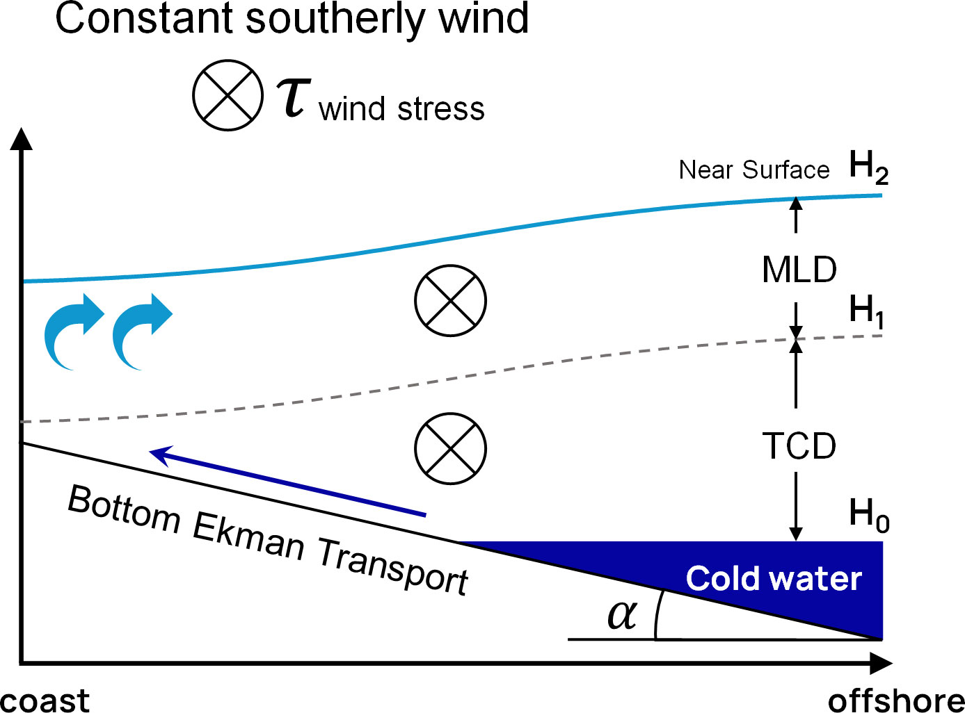
Figure 2 Schematic diagram of the wind-driven upwelling process and advection time (${\tau }_{ad})$ in the Northern Hemisphere.

$\begin{array}{ll}\Gamma = \frac{t_{wind}}{t_{ad}}& (1)\end{array}$

where $t_{wind}$ is the time scale for the duration of an upwelling-favorable wind, and $t_{ad}$ represents advection time. According to Chen et al. (2013), the advection time scale $t_{ad}$ can be scaled as

$\begin{array}{ll}{t}_{ad}=\frac{\rho fd(H_0-H_1)}{\alpha \tau }+\frac{H_1-H_2}{W},& (2)\end{array}$

where the first term is the climbing time scale and the second term is the upwelling time scale. The former refers to the time it takes for cold water to ascend the slope from the thermocline to the transient depth, and the latter refers to the time it takes for cold water to move up from the transient depth to the surface. The factors that make up these two time scales determine the advection time and are the main factors that determine the occurrence of upwelling along with the duration of the wind. In Eq. 2, the climbing time scale is a function of water density ($\rho$), Coriolis parameter ($f$), bottom layer thickness ($d$), alongshore wind stress ($\tau$), bottom slope ($\alpha$), depth of the thermocline ($H_0$), and the switch-over depth between the climbing and upwelling processes (transition depth, $H_1$). The upwelling time scale consists of the transition depth, sea surface ($H_2$), and average vertical velocity over the upwelling region ($W$). $d=\pi \sqrt{2A_z/f}$ and $W=\tau /(\rho fL)$, where $A_z=0.01\tau /(\rho f)$ is the vertical eddy viscosity and $L=0.75\pi (\sqrt{2A_z/f})/\alpha$ is the cross-shore length scale of upwelling, which are empirical formula proposed by Chen et al. (2013).

Ultimately, the UA is expressed as a non-dimensional index. Whereas $\Gamma \gg 1$ results in an adequate accumulation of upwelled water at the coast and thus a large offshore transport forms a surface front, $\Gamma \le 1$ results in no front forms owing to a lack of overturning (Jiang et al., 2012; Chen et al., 2013). To calculate the alongshore wind stress ($\tau$), the wind data at each station were decomposed into alongshore and cross-shore components. In addition, the shelf slope, $\alpha$, was calculated as the ratio of the depth of 200 m to the distance between the coastline (0 m depth) and 200 m depth along the cross-shore line (black lines in Figure 1).

2.3 Multiple linear regression

Although UA is ideally defined using analytical equations, determining the contribution of each geophysical factor (input or predictor of UA) is challenging because the form of the analytical equations (Eqs. 1 and 2) is quite complex, especially when estimating the “independent” contribution of each input. By contrast, in a simple linear equation, the contribution and sensitivity of each factor do not depend on other factors. Thus, the independent contributions can be easily determined.

A complex analysis using machine learning (Jebri et al., 2022) requires big data to train the model, and the complexity of the model is high. Therefore, we projected the UA calculated using the original equations (Eqs. 1 and 2) into linear equations via multiple linear regression (MLR). To quantify the contribution of four geophysical factors ($t_{wind}$, $\text{τ}$, MLD, and TCD) to the upwelling occurrence, a multivariable linear regression model was applied according to the following formula:

$\begin{array}{ll}\Gamma ={\beta }_0+{\beta }_1{t}_{wind}+{\beta }_2\text{τ}+{\beta }_{3}MLD+{\beta }_{4}TCD+\mathrm{\epsilon ,}& (3)\end{array}$

where Γ is the dependent variable calculated from the equations in the previous section, $MLD=H_1-H_2$, and $TCD=H_0-H_1$. The parameter ${\beta }_0$ is a constant, ${\beta }_1\cdots {\beta }_4$ are the regression coefficients for the independent variables, and $\epsilon$ is the error term.

Predictors in the MLR model must be independent of each other to yield correct results. We tested this for each predictor by calculating the variance inflation factor (VIF), which is an indicator of strong correlations between predictors; a VIF<10 indicates no strong relationship between the independent variables (Robinson and Schumacker, 2009). All input variables used in the MLR model did not have multicollinearity (VIF<10) and thus no significant dependency each other. The predictors used in MLR are not independent of one another regarding physics. In particular, MLD and TCD depend on the wind ($t_{wind}$ and $\tau$); vertical mixing that determines MLD is predominantly forced by wind at the surface layer, and TCD is controlled by the wind as a consequence of upwelling. Nevertheless, in our study area, we observed no statistical dependency issues between the predictors used in MLR, implying that the predictors can be considered independent parameters in terms of statistics. We suspect that the independence between the predictors implies a predominance of unresolved forcing by the UA (Eq. 2), such as atmospheric forcing (heating and cooling) or a current-driven effect that may significantly influence determining the vertical density structure than mixing caused by wind.

The proportional reduction of error (PRE) was used to evaluate the relative contribution of a predictor to the model using the following equation (Judd et al., 2011; Park et al., 2019):

$\begin{array}{ll}PR{E}_i=({\epsilon }_{total}-{\epsilon }_i)/{\epsilon }_{total}*\mathrm{100,}& (4)\end{array}$

where ${\epsilon }_{total}$ is the error in the model computed over all independent variables, ${\epsilon }_i$ is the error in the calculated model after excluding a particular independent variable, and the subscript $i$ represents the index for each predictor ($i$ can be $t_{wind}$, $\text{τ}$, $\text{MLD}$, or $\text{TCD}$). The PRE allows the relative contribution of each independent variable to the total proportional reduction of the error to be calculated.

2.4 Water mass analysis to estimate the fraction of upwelled water mass

The fraction of upwelled water mass was estimated using the Expanded Optimal Multi-Parameter (EOMP) method and compared to physical environments such as upwelling-favorable wind stress and alongshore current intensity. The EOMP method calculates the fractions of specified source water masses in an observation using mixing equations. We defined four water masses in the study area: Surface Saline warm Water (SSW), Surface Fresh warm Water (SFW), Deep cold Eutrophic Water (DEW), and Deep cold Oligotrophic Water (DOW). The governing equations are as follows:

$\begin{array}{ll}\left(\begin{array}{cccc}\begin{array}{l}{T}_{SSW}\\ S_{SSW}\\ {[N{O}_3]}_{SSW}\\ {[P{O}_4]}_{SSW}\\ {[Si{O}_4]}_{SSW}\\ 1\end{array}& \begin{array}{l}{T}_{SFW}\\ S_{SFW}\\ {[N{O}_3]}_{SFW}\\ {[P{O}_4]}_{SFW}\\ {[Si{O}_4]}_{SFW}\\ 1\end{array}& \begin{array}{l}{T}_{DEW}\\ S_{DEW}\\ {[N{O}_3]}_{DEW}\\ {[P{O}_4]}_{DEW}\\ {[Si{O}_4]}_{DEW}\\ 1\end{array}& \begin{array}{l}0\\ 0\\ 16\\ 1\\ 16\\ 0\end{array}\end{array}\right)\left(\begin{array}{l}{w}_1\\ w_2\\ w_3\\ w_4\\ \Delta P\end{array}\right)=\left(\begin{array}{l}{T}_{obs}\\ S_{obs}\\ {[N{O}_3]}_{obs}\\ {[P{O}_4]}_{obs}\\ {[Si{O}_4]}_{obs}\\ 1\end{array}\right)& (5)\end{array}$

where $T_n$, $S_n$, ${[N{O}_3]}_n$, ${[P{O}_4]}_n$, ${[Si{O}_4]}_n$, and $w_n$ are the water temperature, salinity, nitrate, phosphate, silicate concentrations, and the fraction of source water, respectively. The subscript $n$ indicates the index of observations ($obs$) and each source water mass. Eq. 5 is the mixing equation that defines the tracer concentrations of observations as a weighted summation (mixture) of four different source water masses and the non-conservative behavior of nutrient species (photosynthesis and respiration). The system of governing equations is overdetermined and thus solved by a linear least-squares problem solver with a non-negative constraint. However, the non-negative constraint was not applied to the biogeochemical change ($\Delta P$) to resolve photosynthesis and respiration. The governing equations for tracer concentrations are normalized by the standard deviation of the source water characteristics (Glover et al., 2011). However, weighting factors were not induced, followed by all the tracers contributing evenly. Details of the definition of source water characteristics are described in the Supplementary Material (Appendix 1). The temperature and salinity of the surface source water varied monthly in this study, eliminating the influence of surface heat and salinity fluxes. Using the defined upwelled water mass indicator, the relationship with force (e.g., wind stress and geostrophic current intensity) is discussed in Section 3.3.

3 Results

3.1 Evaluation of geophysical factors that determine UA

To evaluate upwelling occurrence in response to geophysical factor variations, the UA was adopted as its indicator. Most indices (e.g., upwelling index; Bakun, 1975) that evaluate upwelling occurrence consider only wind forcing as a decisive factor. A few indices (e.g., CUI; Jacox et al., 2018) that reflect the cross-shore current are unsuitable for the east coast of Korea because strong alongshore currents (e.g., EKWC) are entrained along the coastline throughout the year. However, UA makes it possible to deduce the impact of various geophysical factors because it is calculated using multiple variables such as MLD, TCD, bathymetry slope, wind duration, and wind stress. Additionally, this index has been adopted to analyze coastal upwelling in the study area (Kim et al., 2016; Shin et al., 2017). Thus, to accomplish our purpose, the multivariate index is a reliable proxy to evaluate upwelling occurrence.

Nevertheless, additional temporal comparisons were performed to evaluate whether the estimated UA was adequate. Even though the index was compared with the temperature reduction in this area (Kim et al., 2016; Shin et al., 2017), a temporal comparison between the observed water temperature from the observation station and the UA was additionally performed. The comparison determines whether UA reflects a decrease in sea surface temperature by Ekman transport in the study area because the specific conditions for the calculation of UA were slightly improved (Figure 3). Figure 3 shows the time series of UA and water temperature at four stations [Mukho (Figure 3A), Hupo (Figure 3B), Pohang (Figure 3C), and Ulsan (Figure 3D) marked as red triangles in Figure 1 and their corresponding observation stations S16, S10, S07, and S03, respectively] from 2012 to 2018. Gray lines indicate the water temperature anomaly at the observation station (seasonality is removed by subtracting the 60-day moving averaged component), and the black and red lines indicate $\Gamma \le 1$ and $\Gamma >1$ (i.e., upwelling occurrence), respectively. The water temperature reduction corresponds to the red line of the UA. Even though the magnitude of the reduction is not quantitatively proportional to the increase in the index, the sea surface temperature largely falls in response to the variation in the index when UA is >1. In addition, coastal upwelling mainly occurred during the boreal summer season at all stations, showing a distinct seasonality frequently reported in this area (Seung, 1974; Suh et al., 2001; Shin, 2019). A summer case in 2017 (Figures 3E–H) clearly shows that the water temperature in response to upwelling based on UA reflects the upwelled cold water on the sea surface.

FIGURE 3

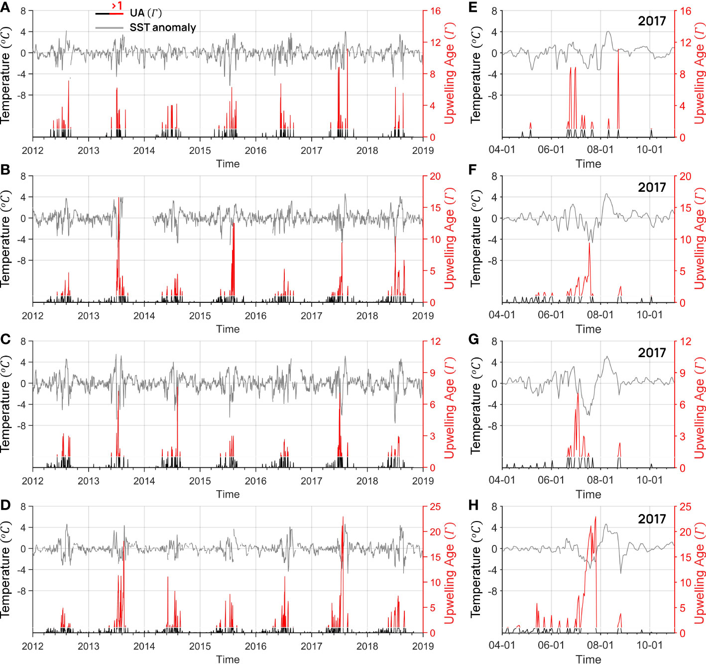
Figure 3 Time series of upwelling age (UA) and sea surface temperature anomaly of (A, E) Mukho [S16], (B, F) Hupo [S10], (C, G) Pohang [S07], and (D, H) Ulsan [S03] (A–D) from 2012 to 2018 and (E–H) from April to October 2017 (refer to Figure 1 for the specific locations). Gray lines indicate the water temperature anomaly derived from stations, and black and red lines indicate UA below and above 1, respectively.

The bathymetry slope plays a critical role in the development of upwelling in favorable environments (Jiang et al., 2012; Chen et al., 2013). Accordingly, the bathymetry slope should influence the upwelling under similar conditions. Eq. 2 shows that $t_{ad}$ decreased as the bottom slope $\alpha$ increased; as a result, $\Gamma$ increased (Eq. 1) as $\alpha$ increased. Therefore, UA predicted that upwelling was proportional to the bottom slope. In terms of the entire east coast of Korea, including both the southern and northern regions, there was no significant relationship between shelf slopes and upwelling frequency (Figure 4). However, a strong positive correlation was observed once the stations were classified into southern (below S14; blue circles in Figure 4) and northern (above S15; reddish circles in Figure 4) regions. Thus, these two regions were under two different conditions for upwelling occurrence, except for the bathymetry slope. Furthermore, the upwelling occurrences in the southern region were larger than those in the northern region, implying that the different conditions result in the southern region having a more upwelling-favorable environment than the northern region.

FIGURE 4

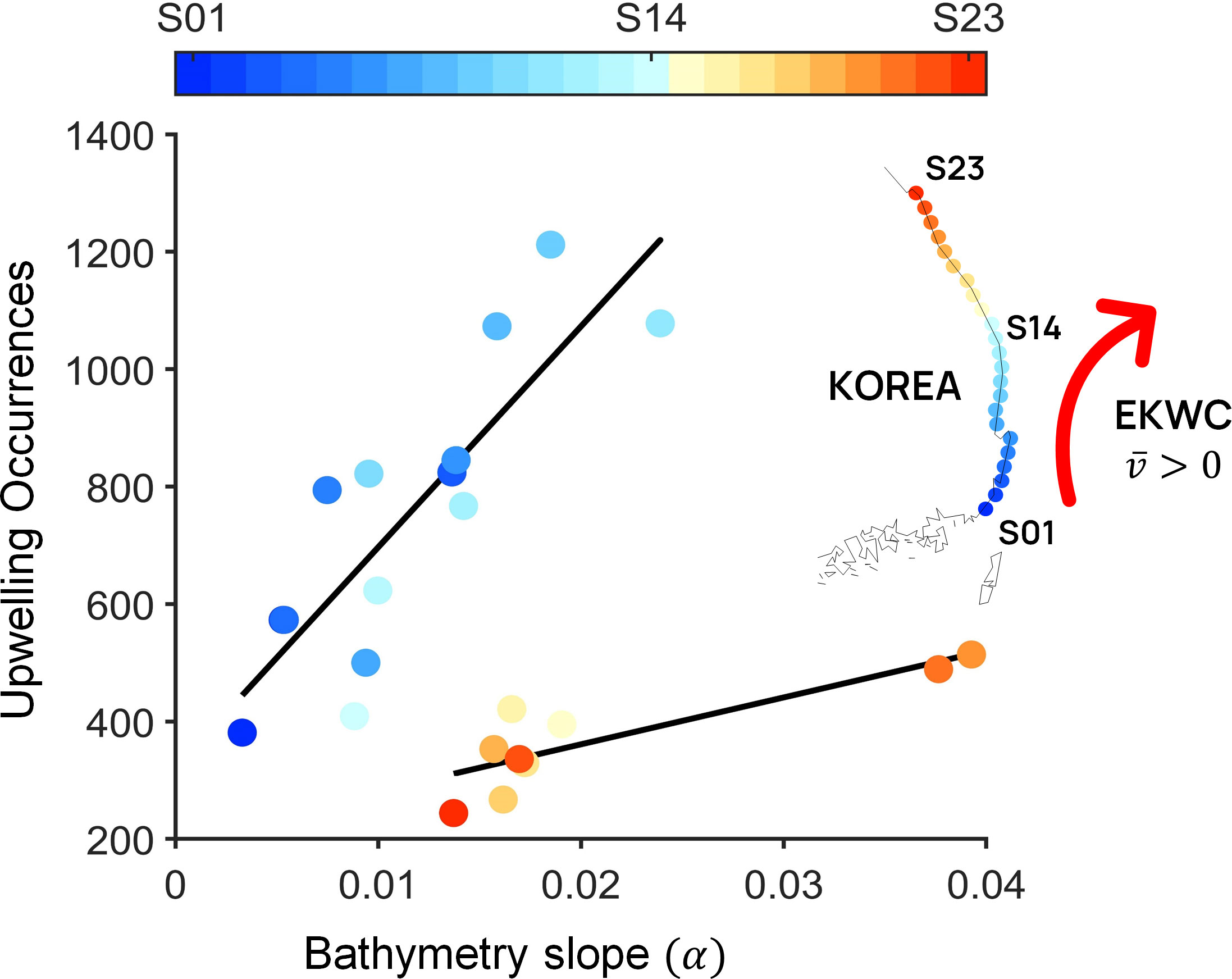
Figure 4 Relationships between upwelling occurrences and bathymetry slopes. Southern and northern regions are represented by a bluish and reddish color, respectively. Data are based on observations from KHOA (1993 to 2018).

3.2 MLR analysis and contribution of wind and isopycnic parameters to UA

In addition to the effect of bathymetry slopes on upwelling occurrence, other time-dependent geophysical changes must be considered. As mentioned above, the geophysical elements ($t_{wind}$, $\tau$, MLD, and TCD) used to calculate UA were evaluated using MLR, and the relative contribution of each element to upwelling events was estimated using PRE (Figure 5). It is worth noting that the wind stress ranges are in the order of 0.01 to 0.1 $\text{N}/{\text{m}}^2$ to develop wind-driven upwelling when UA is larger than one for several days. Although alongshore wind duration is a significant element for UA, the impact of alongshore wind stress, MLD, and TCD was mainly analyzed because our analysis focused on the contribution to advection time $t_{ad}$, which represents the time scale for the bottom water to reach the surface layer. The contribution of wind stress in the southern region (especially from S01 to S03, which corresponds to GU) is significantly smaller than that in the northern region (Figure 5). As a result, the contribution of the subsurface vertical density structure (including both MLD and TCD) is dominant in the southern regions. The contribution from wind stress gradually increased as the latitude increased. The contribution of wind stress from S01 to S03 of the GU was<20% and those of the vertical density structure of the region accounted for >80%. Correspondingly, the contribution of wind stress was negligible in the southern region and gradually increased in the northern region.

FIGURE 5

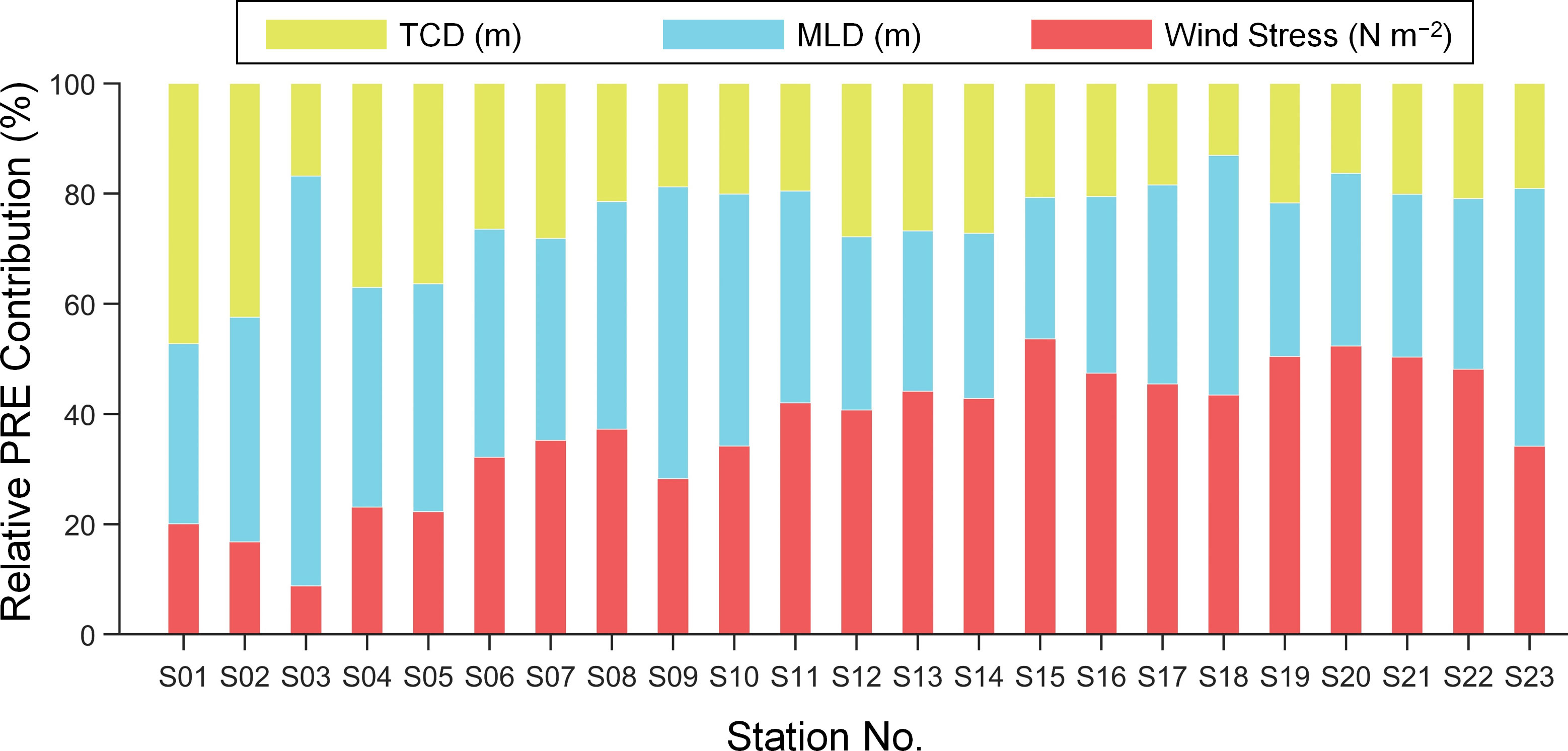
Figure 5 Bar charts of relative contribution rates among factors. The proportional reduction of error (PRE) indicates the contributions of each factor to the upwelling occurrence. Data are based on observations from KHOA (1993 to 2018).

The analysis of the UA shows that the southern region (especially the GU) showed differences with the northern region regarding upwelling occurrence, bathymetry slope (Figure 4), and contribution of the other input variables (Figure 5). The southern region of the GU is adjacent to the Korea Strait and has a gentle slope and a shallow depth (<200 m). In addition, the EKWC, a branch of the Tsushima Warm Current, is consistently entrained through the strait, despite slight seasonal variations. Thus, the vertical density structure in this area can be controlled mainly by the presence of a background current rather than wind variations. In other words, the background alongshore current may play a crucial role in the development of coastal upwelling along the southwestern ES.

3.3 Upwelled water mass fraction and its correlation with alongshore current and wind

Analysis using UA consistently shows that the southern and northern regions were different (Figures 4, 5), and it is hypothesized that the difference was caused by the presence of a persistent current (e.g., EKWC). In this section, the correlation between the fraction of upwelled water mass estimated by the EOMP and alongshore current intensity is discussed. In the case of the correlation between the alongshore geostrophic current and the upwelled water fraction in the northern region, the fraction of upwelled water decreased as the alongshore current increased and was not significantly correlated with the current. However, in another correlation, the stronger the current flows, the higher the upwelled water that accounted for the surface layer in the southernmost region, including observation lines 208 and 207 (Figures 6A, B). These results are evidence for current-driven upwelling in the southern region and support the hypothesis about current-driven upwelling elucidated by UA analysis. Furthermore, the moored observation data in the Korea Strait for 1 year show that onshore flow occurs at the bottom (Teague et al., 2002).

FIGURE 6

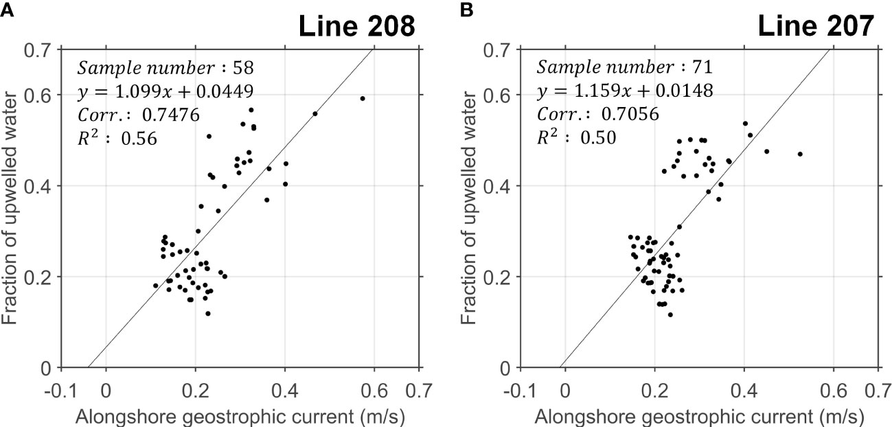
Figure 6 Scatter plot of upwelled water fraction and monthly geostrophic current at (A) Line 208 and (B) Line 207. For observation locations along the lines, refer to Figure 1. Data are based on observations from NIFS (1993 to 2018).

The Burger number $S=\alpha N/f$ [where $h$ is water depth, $N={(-(g/{\rho }_0)\partial \rho \text{'}/\partial z)}^{1/2}$ is the buoyancy frequency, and $f$ is the Coriolis frequency] is a key non-dimensional number controlling many geophysical coastal phenomena, including wind-driven upwelling (Lentz and Chapman, 2004) and persistent alongshore currents over the shelf (Chapman, 2002). Although the alongshore wind stress showed a positive correlation with the fraction of upwelled water mass at all stations along the coast (Figure 7A), the correlation pattern between the upwelled water mass fraction and the alongshore geostrophic current (Figure 7B) matched the Burger number (Figure 7C). The northern region, with a high Burger number, had a relatively weak negative correlation, and the southern region, with a low Burger number, had a significant positive correlation. This implies that the Burger number plays an important role in controlling current-driven upwelling. In the following section, we discuss the theoretical background of wind- and current-driven upwelling and the role of stratification and the Burger number in current-driven upwelling.

FIGURE 7

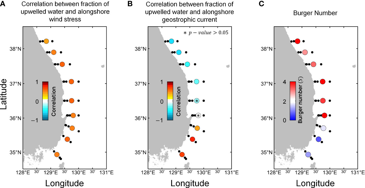
Figure 7 Scatter plot of (A) correlation between upwelling water fraction and alongshore wind stress, (B) correlation between upwelling water fraction and alongshore geostrophic current, and (C) Burger number, $S=\frac{\alpha N}{f}.$ Data are based on observations from NIFS (1993 to 2018).

4 Discussion

We describe the dynamics of the coastal upwelling process, and the details of the compensational flow are analyzed based on momentum equations and not volume compensation by surface Ekman transport. As reviewed by Brink (2016), although the basic concept of upwelling concerning volume conservation (vertical flow compensating offshore surface Ekman current) was realized and verified in the early 20th century, understanding the dynamic mechanism that triggers the compensational flow in terms of momentum balance is still ongoing. Various theoretical studies discussing the dynamic aspect of upwelling have used different assumptions based on research interests and study area characteristics (e.g., spatiotemporal scales). For example, Cushman-Roisin and Beckers (2011) adopted a reduced gravity model that assumes an infinitely deep (relative to the thickness of the surface layer) and motionless subsurface layer. Therefore, their theory systematically excludes the role of bottom friction, and compensational flow is attributed to adjustment flow, which is a consequence of the balance between the Coriolis force and the inertial term (Csanady, 1982). These are reasonable assumptions for stratified large-scale oceans; however, they are inadequate in this study, which focuses on small, shallow marginal oceans influenced by the branches of the WBC. The western boundary region is intrinsically dissipative (Pedlosky, 1987). Furthermore, the time scale for upwelling events in our study area (months) is frequently longer than the frictional adjustment time scale (approximately 5 days), which indicates the importance of bottom friction (Chapman, 2002).

The shallow water equations have been adopted to study upwelling processes (Pringle, 2002; Roughan et al., 2003). For simplicity, we considered a geophysical scale in which the Rossby number was much less than one; thus, the inertial and lateral eddy viscosity terms were not considered. In addition, an anisotropic ocean (Pedlosky, 1987) was assumed, where the alongshore spatial scale (y-direction) was larger than the cross-shore scale (x-direction), $L_x\ll L_y$. In addition, this means that $v$ was much greater than $u$ ($u\approx L_x/T,v\approx L_y/T$). Based on this assumption, the terms associated with vertical eddy viscosity in the x-direction momentum equation were neglected. First, the barotropic limit assuming homogeneous density was analyzed using traditional shallow water equations to explain the dynamics of current-driven upwelling (Section 4.1). The modified shallow water equations by Chapman and Lentz (1997) (Section 4.2) are discussed to understand baroclinic dynamics and the role of stratification. Therefore, the following theoretical analysis provides a general overview of the dynamics of wind-driven and current-driven coastal upwelling processes while explaining the difference between the southern and northern regions caused by background currents and stratification.

4.1 Barotropic current-driven upwelling mechanism

The depth-averaged momentum and continuity equations of the shallow water system with the assumptions mentioned above are as follows:

$\begin{array}{ll}-f\overline{v}=-g\frac{\partial \eta }{\partial x}& (6)\end{array}$

$\begin{array}{ll}f\overline{u}=\frac{{\tau }_y^s}{h{\rho }_0}-\frac{{\tau }_y^b}{h{\rho }_0}& (7)\end{array}$

$\begin{array}{ll}\frac{\partial \eta }{\partial t}+\frac{\partial (h\overline{u})}{\partial x}=0,& (8)\end{array}$

where $\overline{u}$, $\overline{v}$, $h$, $\eta$, ${\rho }_0$, ${\tau }_y^s$, and ${\tau }_y^b$ are the depth-averaged velocity components in the x- and y-directions, water depth, sea level, the constant density component, alongshore surface stress, and bottom stress, respectively. Cross-shore surface and bottom stresses were ignored by $L_x\ll L_y$ ($u\ll v$), which yields a predominantly geostrophic balance (relatively negligible in all the other terms in the cross-shore momentum equation). This is a common assumption in theoretical studies of upwelling in the long alongshore limit (Chapman, 2002; Lentz and Chapman, 2004; Choboter et al., 2005; Choboter et al., 2011) and reasonable assumptions in the study area where there is a predominant alongshore geostrophic current (Kim et al., 2016). If the sea level is assumed to be in a steady state ($\partial \eta /\partial t=0$), $hu$, which indicates that cross-shore transport should be constant in $x$ because $\partial (h\overline{u})/\partial x=0$, is induced from Eq. 8. Considering that the left boundary is bordered and closed by land (${u|}_{x=0}=0$), $\overline{u}=0$ for all $x$. This indicates that cross-shore transport should be zero in the steady-state condition. Thus, Eq. 7 can be rewritten as follows:

$\begin{array}{ll}\overline{u}=\frac{{\tau }_y^s}{fh{\rho }_0}-\frac{{\tau }_y^b}{fh{\rho }_0}=0,& (9)\end{array}$

where ${\tau }_y^s/(fh{\rho }_0)$represents the surface cross-shore Ekman current owing to wind stress and ${\tau }_y^b/(fh{\rho }_0)$ indicates the bottom Ekman current owing to bottom stress. As a result, Eq. 9 indicates that the divergence of the surface Ekman current was compensated by the convergence of the bottom Ekman current (Figure 2). Additionally, it demonstrates the equilibrium between the surface shear stress and the bottom shear stress in the steady state (${\tau }_y^s={\tau }_y^b$). Vertically averaged equations that cannot explicitly resolve vertical structures were used to simplify the mathematical development; however, solutions that explicitly resolve vertical structures are known (Ekman, 1905; Welander, 1957; Estrade et al., 2008; Appendix 2). They are the surface and bottom Ekman currents, which are concentrated at the surface and bottom boundary layers, respectively, and exponentially decay as they get further away from the boundary layers. The bottom stress ${\tau }_y^b$ describes the bottom friction to be specific, as it can be defined as ${\tau }_y^b=\gamma {\rho }_0\overline{v}$ based on the linear frictional bottom boundary condition, where $\gamma$ indicates the bottom friction coefficient in the velocity dimension. Eq. 6 and the bottom boundary condition show that the bottom Ekman current is attributed to geostrophic currents rendered by the pressure gradient formed by surface Ekman transport (Eq. 6). By substituting for the bottom boundary condition, Eq. 6 into Eq. 9 determines the cross-shore sea-level gradient, which is equated as

$\begin{array}{ll} \frac{\partial \eta }{\partial x}=\frac{f}{g}\frac{{\tau }_y^s}{\gamma {\rho }_0}.& (10)\end{array}$

Eq. 10 represents the cross-shore sea-level gradient perturbed by the surface Ekman transport. The alongshore velocity component, which is the geostrophic current based on Eq. 6, during upwelling, a well-known upwelling jet (Kämpf and Chapman, 2016), is defined as $\overline{v}=(f/g)\partial \text{η}/\partial x={\tau }_y^s/(\gamma {\rho }_0)$. The following descriptions describe how coastal wind-driven upwelling was driven: the divergence of the surface Ekman current decreased sea level at the coastal ocean based on the depth-integrated continuity equation (Eq. 8), and the alongshore geostrophic current was generated by the perturbed sea-level gradient and was responsible for the bottom frictional stress and rendering of the bottom Ekman current, which compensated for the divergence of the surface Ekman current (Figure 2).

The momentum balance of the shallow water equations shows that the compensating current was the bottom Ekman current, which responds to the friction of the alongshore currents. Therefore, this implies that coastal upwelling occurred due to the persistent alongshore current, even if the alongshore wind did not flow (Figure 8A). When ${\tau }_y^s$ is neglected, and $\overline{v}={\overline{v}}_b$, which is a constant representing the presence of a persistent background current, Eq. 7 with the bottom boundary condition is induced as follows:

FIGURE 8

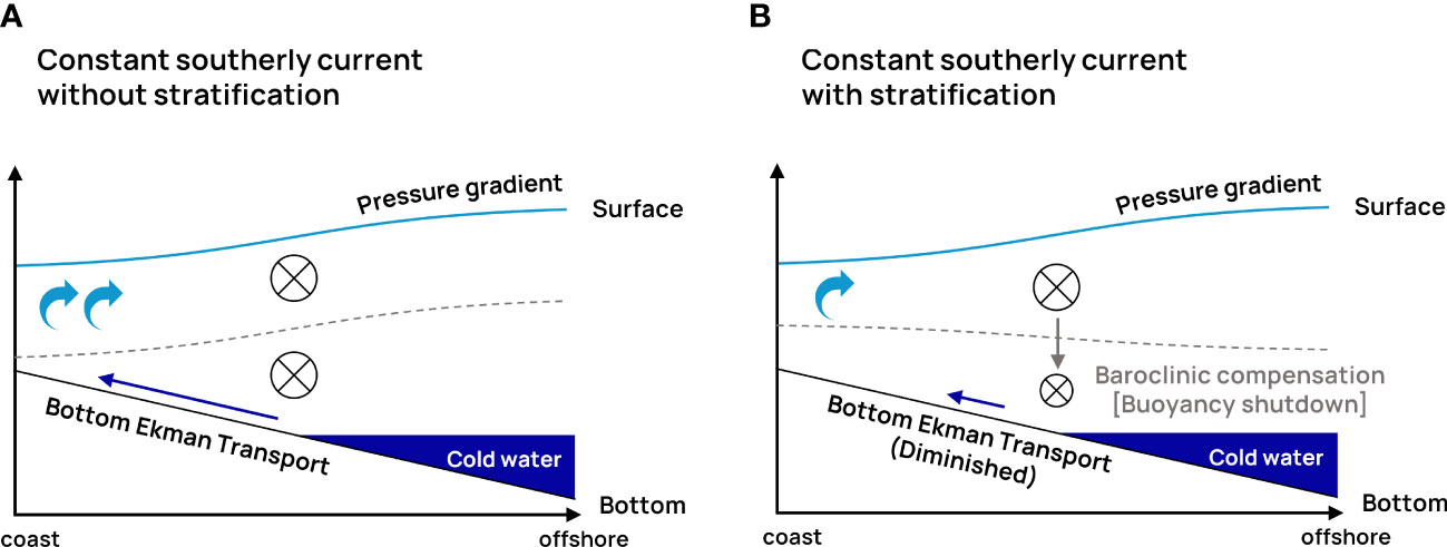
Figure 8 Schematic diagrams of (A) current-driven upwelling processes without stratification (barotropic) and (B) current-driven upwelling processes with stratification (baroclinic).

$\begin{array}{ll}\overline{u}=-\frac{\gamma }{hf}{\overline{v}}_b,& (11)\end{array}$

This indicates that the bottom Ekman current was caused by the persistent alongshore current ${\overline{v}}_b$ (Figure 8A). Therefore, strong and persistent alongshore currents (e.g., WBC) result in transport by bottom friction (Oke and Middleton, 2000; Roughan et al., 2003) and thus develop current-driven upwelling. The EKWC was entrained along the coast of Korea and was enhanced during the prolific upwelling season. Thus, we expect current-driven upwelling to be dominant along a certain coast of Korea.

Eq. 11 implies that the basic concept of current-driven upwelling is imperfect because no flow compensates for the onshore bottom Ekman current. In terms of a steady-state and constant-density ocean, one of the forces ignored in the alongshore momentum equation is expected to generate a compensational flow. Even though the alongshore pressure gradient term was ignored in Eq. 11 for simplicity, it cannot be easily ignored because the scale of the term is intrinsically on the order of one. Therefore, the flow compensating the onshore Ekman current from the background alongshore current was attributed to the barotropic cross-shore geostrophic current, similar to Marchesiello and Estrade (2010).

4.2 Baroclinic current-driven upwelling and the role of stratification

To discuss the baroclinic dynamics of current-driven upwelling with stratification, a modified shallow water equation was adopted (Chapman and Lentz, 1997; Chapman, 2002). The alongshore and cross-shore momentum equations can be written as follows:

$\begin{array}{ll}-fv=-\left(g\frac{\partial \eta }{\partial x}-\frac{g}{{\rho }_0}\frac{\partial \rho \text{'}}{\partial x}z\right)& (12)\end{array}$

$\begin{array}{ll}f\overline{u}=-\frac{\gamma }{h}{v|}_{z=-h},& (13)\end{array}$

where the cross-shore momentum equation (Eq. 12) was not vertically averaged, and the alongshore wind stress in Eq. 13 was ignored to focus on the current-driven upwelling. Substituting Eq. 12 into Eq. 13 yields

$\begin{array}{ll}\overline{u}=-\frac{\gamma }{hf}\left({\overline{v}}_b+\frac{gh}{f{\rho }_0}\frac{\partial \rho \text{'}}{\partial x}\right).& (14)\end{array}$

Note that ${\overline{v}}_b=(g/f) (\partial \eta /\partial x)$ is the background barotropic geostrophic current, which is a given constant, and the density gradient $\partial \rho /\partial x$ is negative in the environment of the study area (especially during upwelling events) and assumed to be constant, similar to Lentz and Chapman (2004). The cross-shore current component described by Eq. 14 is in the bottom Ekman current, based on Eq. 13. The additional terms related to the density gradient in Eq. 14, relative to Eq. 11, which does not consider stratification, indicate a baroclinic geostrophic current (thermal wind) component. As the stratification intensity increased (more negative density gradient), the alongshore current at the bottom ${v|}_{z=-h}$ became weaker than in the barotropic case without stratification because the barotropic velocity component ${\overline{v}}_b$ was canceled by the baroclinic component $gh/(f{\rho }_0)\partial \rho \text{'}/\partial x$ in Eq. 14 (Figure 8B). This alongshore current attenuation near the bottom is known as baroclinic compensation (Lee and Na, 1985; Jacobs et al., 2001) or buoyancy shutdown (Chapman, 2002). As a result, the cross-shore Ekman current caused by the alongshore current at the bottom (Eq. 13) was weakened and represented the bottom Ekman layer arrest process (MacCready and Rhines, 1993; Brink and Lentz, 2010). Consequently, Eq. 14 implies that the current-driven upwelling decreases as stratification increases. Appendix 2 provides the analytical solution for resolving the vertical structure of the stratified current-driven upwelling; however, the dynamics described by the solution are not different from those shown by the vertically averaged equations (Eqs. 13 and 14, respectively).

The thermal wind term is frequently scaled as the Burger number. Specifically, Lentz and Chapman (2004) showed an empirical relation between the lateral density gradient and buoyancy frequency, which is given as:

$\begin{array}{ll}\frac{g}{{\rho }_0}\frac{\partial \rho \text{'}}{\partial x}\approx -afN,& (15)\end{array}$

where $a\approx 0.25$ is a proportional coefficient. The relative dominance of the thermal wind component on the barotropic geostrophic using Eq. 14 can be scaled as

$\begin{array}{ll}O\left(\frac{gh}{f{\rho }_0}\frac{\partial {\rho }^{\prime }}{\partial x}/{\overline{v}}_b\right)=\frac{aS}{{\overline{v}}_b/(f{L}_x)}=a\left(\frac{L_x}{L_y}\right)\frac{S}{Ro},& (16)\end{array}$

where $L_x/L_y$ is the aspect ratio and $R_o=1/(fT)$ is the Rossby number. This can be considered a non-dimensional number representing the dominance of the current-driven current. If stratification is negligible and the slope is gentle ($S\approx 0$), the system becomes barotropic, and the alongshore current effectively generates a frictional bottom Ekman current. In contrast, for highly stratified environments over steep slopes ($S\approx 1$), the alongshore current is attenuated at the bottom because barotropic velocity is canceled by baroclinic velocity, and the cross-shore bottom Ekman current is not generated by the stratified alongshore current, and thus the non-dimensional number (Eq. 16) indicates the dominance of the current-driven upwelling. If the number is zero, the alongshore current generates a cross-shore bottom Ekman current, indicating dominant current-driven upwelling. In contrast, current-driven upwelling becomes negligible when the number is on the order of one because the bottom alongshore current is attenuated, and the bottom cross-shore Ekman current caused by the alongshore current weakens. A dimensionless number (Eq. 16) is consistent with the results of Chapman (2002), who showed that the governing equation for the alongshore current over a stratified shelf is controlled by two different non-dimensional numbers: the Rossby and Burger numbers. Consequently, the dimensionless number in Eq. 16 implies that the southern region had a dominant alongshore current and small Burger number, and thus current-driven upwelling may be considerable. However, the northern region, which had a relatively weak alongshore current and a high Burger number, may have been less affected by the current-driven upwelling. The correlation between the alongshore current and upwelled water mass fraction strongly agrees with the dynamics proposed in this study; a high correlation was observed in the southern region, where the Burger number was small, and vice versa in the northern region (Figure 7C). As a result, current-driven upwelling occurred in the southern region below 35° N.

5 Conclusions

We gained insights into the dominant upwelling processes under different local conditions in the southern and northern regions of the southwest ES by analyzing the contributions of major geophysical factors. The coastal upwelling off the study area was mainly evaluated using the wind-forcing impact. The southwesterly wind blowing in the boreal summer was mainly responsible for the compensation of bottom water to the surface, inducing cross-shore Ekman transport. However, the frequencies of upwelling showed regionally distinguishable relationships in response to bathymetry slopes (S01–S14 and S15–S23). Furthermore, according to the evaluation of the variable impact of upwelling, although wind forcing was the dominant factor in the northern region (>S14), upwelling in the southern region (<S14) was considerably smaller. These results imply that there are critical factors underlying the differences between the southern and northern regions.

In addition, a branch of the Tsushima Current (EKWC) gradually reinforced from the boreal summer to winter along the southwest ES (Teague et al., 2002; Kim et al., 2006). Accompanied by the robust boundary current, the current-driven upwelling resulted from the onshore bottom transport caused by bottom friction. Additionally, it should be noted whether the alongshore surface currents can be maintained at the bottom (barotropic). The theoretical analysis in Section 4 shows that the current-driven upwelling decreased as the Burger number increased because the alongshore current at the bottom diminished due to buoyancy shutdown and bottom Ekman arrest. In conclusion, it is inferred that the southern region had a small Burger number and was governed by predominant current-driven upwelling, whereas the northern region, which had a high Burger number, was rarely influenced by the currents and was thus governed by wind-driven upwelling.

Data availability statement

The original contributions presented in the study are included in the article/Supplementary Material. Further inquiries can be directed to the corresponding author.

Author contributions

Conceptualization: DK, J-GC, and JP. Data curation: DK and J-GC. Methodology: DK, J-GC, JP, and Y-HJ. Formal analyses: DK and J-GC. Writing the original draft: DK and J-GC. Writing, review, and editing: DK, J-GC, JP, J-IK, M-HK, and Y-HJ. Supervision: Y-HJ. All authors contributed to the article and approved the submitted version.

Funding

This research was supported by a National Research Foundation of Korea (NRF) grant funded by the Korean government (MSIP) (NRF-2018R1A2B2006555) for the project titled “Development of technology using analysis of ocean satellite images” (20210046). This study was partially supported by the Korea Institute of Marine Science & Technology Promotion (KIMST), funded by the Ministry of Oceans and Fisheries, Korea (20180447, Improvements in ocean prediction accuracy using numerical modeling and artificial intelligence technology).

Conflict of interest

The authors declare that the research was conducted in the absence of any commercial or financial relationships that could be construed as a potential conflict of interest.

Publisher’s note

All claims expressed in this article are solely those of the authors and do not necessarily represent those of their affiliated organizations, or those of the publisher, the editors and the reviewers. Any product that may be evaluated in this article, or claim that may be made by its manufacturer, is not guaranteed or endorsed by the publisher.

Supplementary material

The Supplementary Material for this article can be found online at: https://www.frontiersin.org/articles/10.3389/fmars.2023.1165366/full#supplementary-material

References

Alvarez I., Gomez-Gesteira M., DeCastro M., Gomez-Gesteira J., Dias J. (2010). Summer upwelling frequency along the western cantabrian coast from 1967 to 2007. J. Mar. Syst. 79 (1-2), 218–226. doi: 10.1016/j.jmarsys.2009.09.004

CrossRef Full Text | Google Scholar

Bakun A. (1975). Daily and weekly upwelling indices, west coast of north america 1967-73. U.S. NOAA technical report National Marine Fisheries Service SSRF, Vol. 693 (Washington, DC: NOAA).

Google Scholar

Brink K. (2016). Cross-shelf exchange. Annu. Rev. Mar. Sci. 8, 59–78. doi: 10.1146/annurev-marine-010814-015717

CrossRef Full Text | Google Scholar

Brink K. H., Lentz S. J. (2010). Buoyancy arrest and bottom ekman transport. part I: steady flow. J. Phys. Oceanography 40 (4), 621–635. doi: 10.1175/2009JPO4266.1

CrossRef Full Text | Google Scholar

Chang K.-I., Hogg N. G., Suk M.-S., Byun S.-K., Kim Y.-G., Kim K. (2002). Mean flow and variability in the southwestern East Sea. Deep Sea Res. Part I: Oceanographic Res. Papers 49 (12), 2261–2279. doi: 10.1016/S0967-0637(02)00120-6

CrossRef Full Text | Google Scholar

Chapman D. C. (2002). Deceleration of a finite-width, stratified current over a sloping bottom: frictional spindown or buoyancy shutdown? J. Phys. Oceanography 32 (1), 336–352. doi: 10.1175/1520-0485(2002)032<0336:DOAFWS>2.0.CO;2

CrossRef Full Text | Google Scholar

Chapman D. C., Lentz S. J. (1997). Adjustment of stratified flow over a sloping bottom. J. Phys. Oceanography 27 (2), 340–356. doi: 10.1175/1520-0485(1997)027<0340:AOSFOA>2.0.CO;2

CrossRef Full Text | Google Scholar

Chen Z., Yan X.-H., Jiang Y., Jiang L. (2013). Roles of shelf slope and wind on upwelling: a case study off east and west coasts of the US. Ocean Model. 69, 136–145. doi: 10.1016/j.ocemod.2013.06.004

CrossRef Full Text | Google Scholar

Choboter P. F., Duke D., Horton J. P., Sinz P. (2011). Exact solutions of wind-driven coastal upwelling and downwelling over sloping topography. J. Phys. Oceanography 41 (7), 1277–1296. doi: 10.1175/2011JPO4527.1

CrossRef Full Text | Google Scholar

Choboter P. F., Samelson R. M., Allen J. S. (2005). A new solution of a nonlinear model of upwelling. J. Phys. oceanography 35 (4), 532–544. doi: 10.1175/JPO2697.1

CrossRef Full Text | Google Scholar

Csanady G. T. (1981). “Circulation in the coastal ocean,” in Advances in geophysics, vol. 23. (Dordrecht: Springer), 101–183. doi: 10.1007/978-94-017-1041-1

CrossRef Full Text | Google Scholar

Cushman-Roisin B., Beckers J.-M. (2011). Introduction to geophysical fluid dynamics: physical and numerical aspects (Cambridge, MA: Academic press).

Google Scholar

Ekman V. (1905). On the influence of the earth's rotation on ocean currents. Arkiv Matematik Astronomi Fysik 2:52.

Google Scholar

Estrade P., Marchesiello P., De Verdière A. C., Roy C. (2008). Cross-shelf structure of coastal upwelling: a two–dimensional extension of ekman's theory and a mechanism for inner shelf upwelling shut down. J. Mar. Res. 66 (5), 589–616. doi: 10.1357/002224008787536790

CrossRef Full Text | Google Scholar

García-Reyes M., Largier J. L., Sydeman W. J. (2014). Synoptic-scale upwelling indices and predictions of phyto-and zooplankton populations. Prog. Oceanography 120, 177–188. doi: 10.1016/j.pocean.2013.08.004

CrossRef Full Text | Google Scholar

Glover D. M., Jenkins W. J., Doney S. C. (2011). Modeling methods for marine science (Cambridge, UK: Cambridge University Press).

Google Scholar

Huyer A. (1983). Coastal upwelling in the California current system. Prog. Oceanography 12 (3), 259–284. doi: 10.1016/0079-6611(83)90010-1

CrossRef Full Text | Google Scholar

Jacobs G., Perkins H., Teague W., Hogan P. (2001). Summer transport through the tsushima-Korea strait. J. Geophysical Research: Oceans 106 (C4), 6917–6929. doi: 10.1029/2000JC000289

CrossRef Full Text | Google Scholar

Jacox M., Edwards C. (2011). Effects of stratification and shelf slope on nutrient supply in coastal upwelling regions. J. Geophysical Research: Oceans 116 (C3). doi: 10.1029/2010JC006547

CrossRef Full Text | Google Scholar

Jacox M. G., Edwards C. A., Hazen E. L., Bograd S. J. (2018). Coastal upwelling revisited: Ekman, Bakun, and improved upwelling indices for the US West coast. J. Geophysical Research: Oceans 123 (10), 7332–7350. doi: 10.1029/2018JC014187

CrossRef Full Text | Google Scholar

Jebri F., Srokosz M., Jacobs Z. L., Nencioli F., Popova E. (2022). Earth observation and machine learning reveal the dynamics of productive upwelling regimes on the agulhas bank. Front. Mar. Sci. 9. doi: 10.3389/fmars.2022.872515

PubMed Abstract | CrossRef Full Text | Google Scholar

Ji R., Jin M., Li Y., Kang Y.-H., Kang C.-K. (2019). Variability of primary production among basins in the East/Japan Sea: role of water column stability in modulating nutrient and light availability. Prog. Oceanography 178, 102173. doi: 10.1016/j.pocean.2019.102173

CrossRef Full Text | Google Scholar

Jiang L., Breaker L. C., Yan X.-H. (2012). Upwelling age: an indicator of local tendency for coastal upwelling. J. Oceanography 68 (2), 337–344. doi: 10.1007/s10872-011-0096-2

CrossRef Full Text | Google Scholar

Judd C. M., McClelland G. H., Ryan C. S. (2009). Data analysis: A model comparison approach (New York: Routledge).

Google Scholar

Jung J., Cho Y.-K. (2020). Persistence of coastal upwelling after a plunge in upwelling-favourable wind. Sci. Rep. 10 (1), 1–9. doi: 10.1038/s41598-020-67785-x

PubMed Abstract | CrossRef Full Text | Google Scholar

Kämpf J., Chapman P. (2016). Upwelling systems of the world (Cham: Springer).

Google Scholar

Kara A. B., Rochford P. A., Hurlburt H. E. (2000). An optimal definition for ocean mixed layer depth. J. Geophysical Research: Oceans 105 (C7), 16803–16821. doi: 10.1029/2000JC900072

CrossRef Full Text | Google Scholar

Kim I. N. (2015). Estimating denitrification rates in the East/Japan Sea using extended optimum multi-parameter analysis. Terrestrial Atmospheric Oceanic Sci. 26, 145–152. doi: 10.3319/TAO.2014.09.24.01(Oc)

CrossRef Full Text | Google Scholar

Kim D.-W., Jo Y.-H., Choi J.-K., Choi J.-G., Bi H. (2016). Physical processes leading to the development of an anomalously large cochlodinium polykrikoides bloom in the East sea/Japan sea. Harmful Algae 55, 250–258. doi: 10.1016/j.hal.2016.03.019

PubMed Abstract | CrossRef Full Text | Google Scholar

Kim D.-S., Kim D.-H. (2008). Numerical simulation of upwelling appearance near the southeastern coast of Korea. J. Korean Soc. Mar. Environ. Saf. 14 (1), 1–7.

Google Scholar

Kim Y. H., Kim Y. B., Kim K., Chang K. I., Lyu S. J., Cho Y. K., et al. (2006). Seasonal variation of the Korea strait bottom cold water and its relation to the bottom current. Geophysical Res. Lett. 33 (24). doi: 10.1029/2006GL027625

CrossRef Full Text | Google Scholar

Kim I. N., Lee T. S. (2004). Physicochemical properties and the origin of summer bottom cold waters in the Korea strait. Ocean Polar Res. 26 (4), 595–606. doi: 10.4217/OPR.2004.26.4.595

CrossRef Full Text | Google Scholar

Kim K., Lyu S. J., Kim Y.-G., Choi B. H., Taira K., Perkins H. T., et al. (2004). Monitoring volume transport through measurement of cable voltage across the Korea strait. J. Atmospheric Oceanic Technol. 21 (4), 671–682. doi: 10.1175/1520-0426(2004)021<0671:MVTTMO>2.0.CO;2

CrossRef Full Text | Google Scholar

Kim I. N., Min D. H., Kim D. H., Lee T. (2010). Investigation of the physicochemical features and mixing of East/Japan Sea intermediate water: an isopycnic analysis approach. J. Mar. Res. 68 (6), 799–818. doi: 10.1357/002224010796673849

CrossRef Full Text | Google Scholar

Lee J.-C. (1983). Variations of sea level and sea surface temperature associated with and wind-induced upwelling in the southeast coast of Korea in summer. J. Korean Ocean. Soc 18, 149–160.

Google Scholar

Lee D.-K., Kwon J.-I., Hahn S.-B. (1998). The wind effect on the cold water formation near gampo-ulgi coast. Korean J. Fisheries Aquat. Sci. 31 (3), 359–371.

Google Scholar

Lee J.-C., Na J.-Y. (1985). Structure of upwelling off the southease coast of Korea. J. Korean Soc. Oceanography 20 (3), 6–19.

Google Scholar

Lentz S. J., Chapman D. C. (2004). The importance of nonlinear cross-shelf momentum flux during wind-driven coastal upwelling. J. Phys. Oceanography 34 (11), 2444–2457. doi: 10.1175/JPO2644.1

CrossRef Full Text | Google Scholar

MacCready P., Rhines P. B. (1993). Slippery bottom boundary layers on a slope. J. Phys. Oceanography 23 (1), 5–22. doi: 10.1175/1520-0485(1993)023<0005:SBBLOA>2.0.CO;2

CrossRef Full Text | Google Scholar

Marchesiello P., Estrade P. (2010). Upwelling limitation by onshore geostrophic flow. J. Mar. Res. 68 (1), 37–62. doi: 10.1357/002224010793079004

CrossRef Full Text | Google Scholar

Oke P. R., Middleton J. H. (2000). Topographically induced upwelling off eastern Australia. J. Phys. Oceanography 30 (3), 512–531. doi: 10.1175/1520-0485(2000)030<0512:TIUOEA>2.0.CO;2

CrossRef Full Text | Google Scholar

Park J., Kim J. H., Kim H., Hwang J., Jo Y. H., Lee S. H. (2019). Environmental forcings on the remotely sensed phytoplankton bloom phenology in the central Ross Sea polynya. J. Geophysical Research: Oceans 124 (8), 5400–5417. doi: 10.1029/2019JC015222

CrossRef Full Text | Google Scholar

Pedlosky J. (1987). Geophysical fluid dynamics Vol. 710 (New York: Springer). doi: 10.1007/978-1-4612-4650-3

CrossRef Full Text | Google Scholar

Pringle J. M. (2002). Enhancement of wind-driven upwelling and downwelling by alongshore bathymetric variability. J. Phys. Oceanography 32 (11), 3101–3112. doi: 10.1175/1520-0485(2002)032<3101:EOWDUA>2.0.CO;2

CrossRef Full Text | Google Scholar

Robinson C., Schumacker R. E. (2009). Interaction effects: centering, variance inflation factor, and interpretation issues. Multiple linear regression viewpoints 35 (1), 6–11.

Google Scholar

Rossi V., Feng M., Pattiaratchi C., Roughan M., Waite A. M. (2013). On the factors influencing the development of sporadic upwelling in the leeuwin current system. J. Geophysical Research: Oceans 118 (7), 3608–3621. doi: 10.1002/jgrc.20242

CrossRef Full Text | Google Scholar

Roughan M., Oke P. R., Middleton J. H. (2003). A modeling study of the climatological current field and the trajectories of upwelled particles in the East Australian current. J. Phys. Oceanography 33 (12), 2551–2564. doi: 10.1175/1520-0485(2003)033<2551:AMSOTC>2.0.CO;2

CrossRef Full Text | Google Scholar

Seung Y. H. (1974). A dinamic consideration on the temperature distribution in the East coast of Korea in august. J. Korean Soc. Oceanography 9 (2), 52–58.

Google Scholar

Shin C.-W. (2019). Change of coastal upwelling index along the southeastern coast of Korea. Sea 24 (1), 79–91. doi: 10.7850/jkso.2019.24.1.079

CrossRef Full Text | Google Scholar

Shin J. W., Park J., Choi J. G., Jo Y. H., Kang J. J., Joo H., et al. (2017). Variability of phytoplankton size structure in response to changes in coastal upwelling intensity in the southwestern East Sea. J. Geophysical Research: Oceans 122 (12), 10262–10274. doi: 10.1002/2017JC013467

CrossRef Full Text | Google Scholar

Suh Y. S., Jang L.-H., Hwang J. D. (2001). Temporal and spatial variations of the cold waters occurring in the eastern coast of the Korean peninsula in summer season. Korean J. Fisheries Aquat. Sci. 34 (5), 435–444.

Google Scholar

Teague W. J., Jacobs G., Perkins H., Book J., Chang K., Suk M. (2002). Low-frequency current observations in the Korea/Tsushima strait. J. Phys. Oceanography 32 (6), 1621–1641. doi: 10.1175/1520-0485(2002)032<1621:LFCOIT>2.0.CO;2

CrossRef Full Text | Google Scholar

Welander P. (1957). Wind action on a shallow sea: some generalizations of Ekman’s theory. Tellus 9 (1), 45–52.

Google Scholar

Yoo S., Park J. (2009). Why is the southwest the most productive region of the East Sea/Sea of Japan? J. Mar. Syst. 78 (2), 301–315. doi: 10.1016/j.jmarsys.2009.02.014

CrossRef Full Text | Google Scholar