Spatial and seasonal variations of near-inertial kinetic energy in the upper Ross Sea and the controlling factors

1 Introduction

Near-inertial internal waves (NIWs), an important mode of high-frequency variability in the ocean with a lateral scale of 10 to 100 km and a frequency near the local Coriolis frequency ($f_0$), are ubiquitous in the global ocean (Munk and Wunsch, 1998; Alford et al., 2016; Yu et al., 2022). NIWs represent one of the main sources of turbulent mixing in the ocean interior due to their large amount of energy and strong velocity shear in the vertical direction (Hebert and Moum, 1994; Ferrari and Wunsch, 2009; Alford et al., 2016; Lu et al., 2022). Although previous studies show that the NIWs can be generated by various processes, such as the spontaneous emission or breaking of lee waves, wind disturbances represent the most important generation mechanism of NIWs in the ocean (Pollard and Millard, 1970; D'Asaro, 1985; D'Asaro et al., 1995; Firing et al., 1997). The Ross Sea (RS), as one of the most productive regions of the Antarctic marginal sea, is an idealized site for studying sea ice–air interactions and physical–ecological coupling processes (Smith et al., 2012). Since it is subject to Katabatic winds all year round, the study of the effects of wind on the near-inertial kinetic energy in the RS has important implications for understanding the ocean mixing and biogeochemical cycles.

NIWs represent an important pathway for the energy transfer from the wind to ocean mixing process (Munk and Wunsch, 1998; Alford et al., 2016; Hummels et al., 2020). NIWs with high vertical wavenumber (high mode) have small group velocity and likely dissipate locally, while those with low vertical wavenumber (low mode) can propagate away from the source region toward the equator before they break up (Garrett, 2001; Silverthorne and Toole, 2009; Alford et al., 2016). The annual mean global energy flux to wind-generated inertial motion in the surface mixed layer is estimated to be approximately 0.3 to 1.5 TW by using the simple slab models (Watanabe and Hibiya, 2002; Alford, 2003; Jiang et al., 2005; Alford, 2020).

Many studies have investigated the factors influencing the wind-generated near-inertial response. As a linear response to the wind field, wind stress with more energy in the near-inertial band can produce a more intense near-inertial response in the ocean surface mixed layer (Alford et al., 2016). Based on 2,480 moored current-meter records, Alford and Whitmont (2007) showed that there is a seasonal cycle in the near-inertial kinetic energy (NIKE) in both the northern and southern hemispheres. Synoptic activities such as cyclones can play an important in modulating the NIKE (Price, 1981; Shay et al., 1998; Guan et al., 2014).

In the polar region, the response process of NIWs becomes more complicated due to the presence of sea ice. Based on the Ice-Tethered Profiler in the Arctic Ocean, Dosser and Rainville (2016) found that the NIW field was most energetic in summer when sea ice was at a minimum, with a second maximum in early winter during the period of maximum wind speed. The main reason is that the presence of sea ice prevents fluctuations in the wind field from acting directly on the surface ocean. Furthermore, recent studies show that the mixed layer depth (MLD) and low β (latitudinal variation in Coriolis frequency) can also influence NIKE distribution in polar regions (Rainville et al., 2011; Guthrie and Morison, 2021; Subeesh et al., 2022). By comparing near-inertial currents within the mixed layer and NIWs below the mixed layer in the Arctic fjord during austral summer and winter, Subeesh et al. (2022) found that the shallow summer MLD excites the generation of strong near-inertial currents within the mixed layer, which allows NIWs to propagate to deeper regions. Guthrie and Morison (2021) studied the efficiency of simulated near-inertial oscillations in mixed layer forcing by determining the ratio of the pycnocline NIKE to the initial mixed layer NIKE and found that it decreases with decreasing β or increasing latitude.

Only limited studies have investigated NIWs in the Southern Ocean, especially the Antarctic region. Due to the difficulty of polar observation, numerical simulations become a useful tool to study the spatial and temporal distributions of NIKE there. Rath et al. (2014) used a model to examine the spatial and temporal variabilities of near-inertial wind power input and near-inertial energy in the Southern Ocean. Based on a coupled biogeochemical model, Song et al. (2019) showed that NIWs have an important role in modulating the surface vertical mixing and sea–air CO₂ fluxes in the Southern Ocean. The RS (Figure 1) overlies the largest continental shelf in the Southern Ocean and is one of a few locations that form and export Antarctic Bottom Water (Orsi et al., 1999; Gordon et al., 2009). The topography of the RS continental shelf is complex, with banks and troughs interspersed. Brine rejection causes significant changes in MLD in the RS, especially in the polynya regions. At the same time, the Katabatic winds and frequent synoptic wind events also contribute to the change of MLD. In recent years, the RS is experiencing an increase in sea ice extent (Comiso et al., 2011), a decrease in summer ice-free periods (Parkinson, 2002), and stronger southerly winds (Holland and Kwok, 2012). The presence of unique geographic features and complex physical processes also highlights the importance of understanding the near-inertial motions in the RS.

FIGURE 1

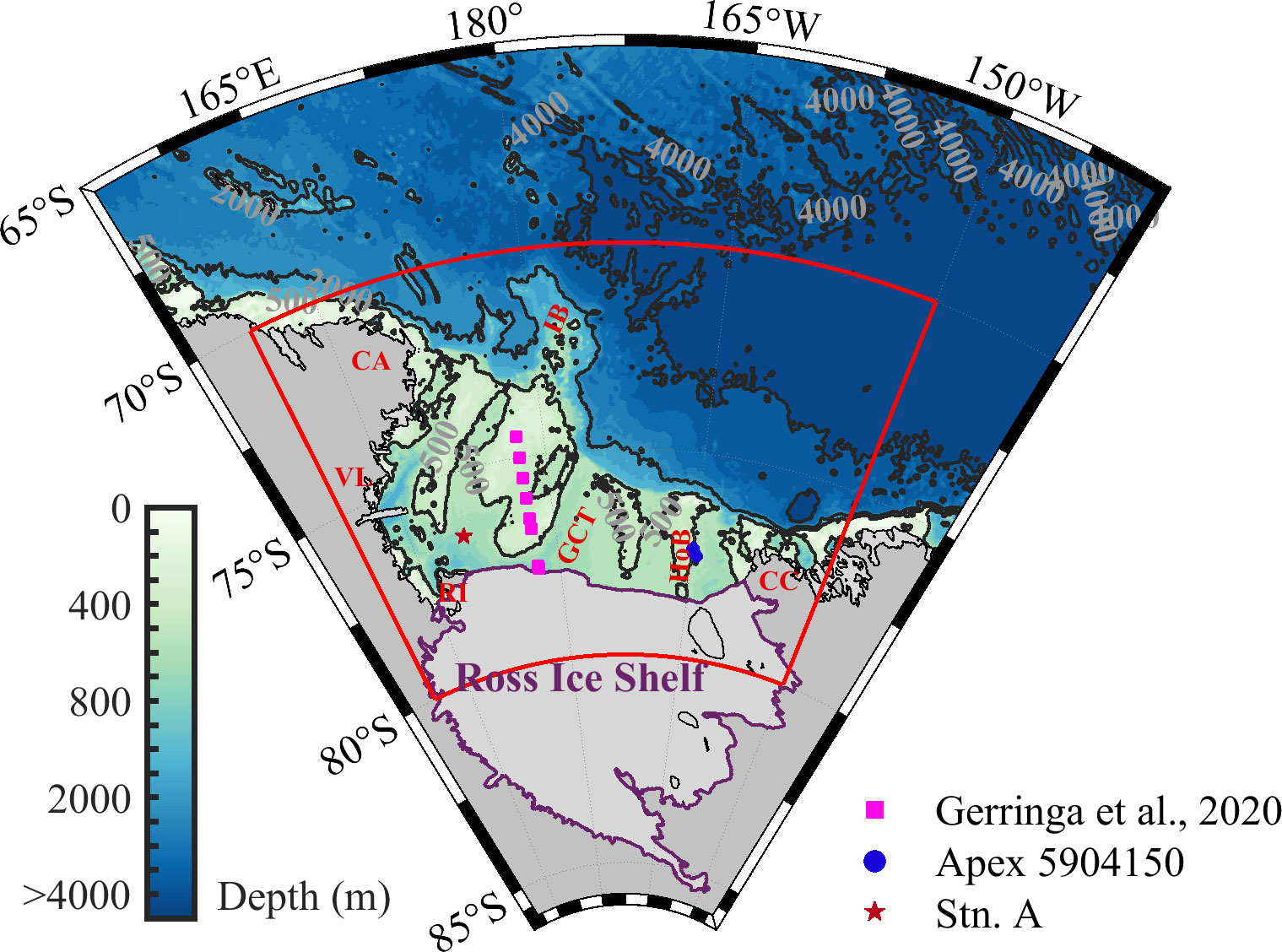
Figure 1 The domain of the ROSE model and bathymetry of RS from Bedmap2. The red curves denote the study area. The magenta points denote the locations of the observation data from Gerringa et al. (2020), which was used for model validation. The red star [Station A (Stn. A)] denotes the location of the presented typical near-inertial response event in Section 3.3. The location of the Apex float (5904150) is shown by purple dots. The gray color represents the isobaths, which represent the values 500, 2,000, and 3,000 in different areas. GCT, Glomar Changer Trough; IB, Iselin Bank; HoB, Houtz Bank; CA, Cape Adare; CC, Cape Colbeck; VL, Victoria Land; RI, Ross Island; RS, Ross Sea.

Based on a three-dimensional numerical simulation in the RS, we investigate the spatial and seasonal variations of NIKE in the RS with the influencing factors discussed. This paper is organized as follows. Section 2 describes the model setting and data processing methods. The model validation, the spatial and seasonal variations of NIKE, and a typical near-inertial response event are investigated in Section 3. Section 4 discusses the influencing factors. The results are summarized in Section 5.

2 Data and methods

2.1 ROSE model

The hourly output from the 1/4° sea-ice physical–biological coupled model based on NEMO3.6-LIM3 with modified PISCES for the RS (Ross Sea Ocean-Sea ice-Ecosystem coupled model, ROSE model) was used to investigate the NIWs in this study. Only the physical outputs from the ROSE model are used in the present study. The model has 75 vertical grids. Specifically, there are 19 layers at the upper 50 m; the layer thickness is 1 m near the surface and increases gradually with depth to approximately 200 m at 6,000 m. The layer thickness of the last layer varies according to the topography. Figure 2 shows the model domain (155°E–140°W; 65°S–86°S) with the red box indicating the focused area in this study. The atmospheric forcing for the model comes from the hourly EAR5 reanalysis product, which includes wind speed, surface wind stress, and heat flux. A hindcast simulation starting from 2009 to 2019 was carried out. The bathymetry of the model is obtained from Bedmap2. The initial 3D ocean temperature and salinity fields are derived from climate state data from the World Ocean Atlas (WOA2018). The initial horizontal current velocity fields, sea surface height, and sea ice data are derived from the Global Reanalysis HYCOM and GLORYS12V1 datasets. Monthly averages from GLORYS12V1 are used for open boundary temperature, salinity, sea surface height, horizontal current field, and sea ice. The open boundary currents of the model are driven by the five subtidal tides (K₁, O₁, M₂, S₂, and N₂), and the tidal data are extracted from the TPXO9 version of the Global Ocean Tidal Model results from Oregon State University (OSU) (https://www.tpxo.net/global/tpxo9-atlas). The model sets different open boundary conditions for barotropic and baroclinic modes. Flather radiation boundary conditions are used for the mean current velocity along the normal depth of the positive pressure mode, while the “sponge layer” is set at 10 grid spacing within the open boundary for the baroclinic current velocity, temperature, and salinity.

FIGURE 2

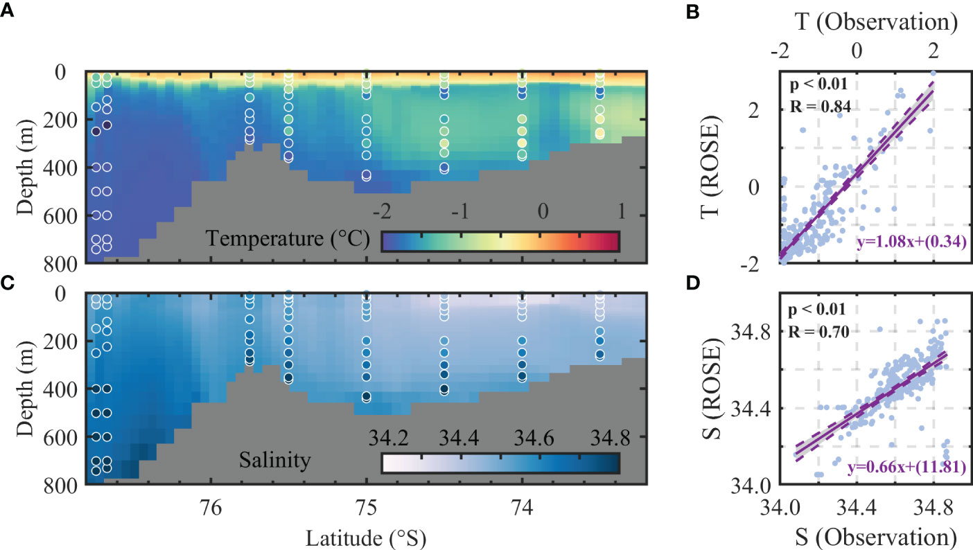
Figure 2 The vertical distribution of temperature (A) and salinity (C) along the transect is shown in Figure 1. The background color represents the ROSE model output. The scatters denote the observation from Gerringa et al. (2020). The scatter plots of temperature and salinity between the (B) observation and (D) simulation results. The solid and dashed purple lines represent the fitted result line and the upper and lower 95% confidence limits, respectively.

In the following study, we used the hourly model output of currents, temperatures, salinities, and MLDs from January to December 2017. The sea ice concentration (SIC) data from the EUMETSAT Ocean and Sea Ice Satellite Application Facility (OSI SAF) were used to validate the model SIC. Please also refer to Table 1 for more details on the data used in this study.

TABLE 1

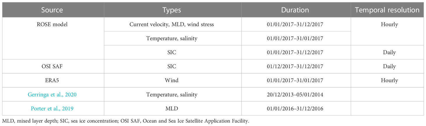
Table 1 The used data and corresponding resolutions.

2.2 Methods

2.2.1 The extraction of near-inertial component

In our study, the barotropic velocity ($U$, $V$) and baroclinic velocity ($u^{\text{'}}$, $v^{\text{'}}$) were calculated as the depth-averaged velocity and the subtraction of the barotropic velocity from the raw velocity ($u$, $v$) (i.e., $u^{\text{'}}$ = $u$ − $U$), respectively. We apply a bandpass filter with a frequency range of 0.9 $f_0$–1.15 $f_0$ to the model-simulated baroclinic velocities to extract the near-inertial component ($u_{bp}^{\text{'}}$ $v_{bp}^{\text{'}}$). $f_0$ is the local inertial frequency, which depends on the latitude. The typical near-inertial frequency in the Ross Sea is from ~1.8797 to ~1.9523 cpd (70.0233°S to 77.4609°S). The mixed layer-integrated NIKE was calculated as follows:

$\begin{array}{ll}\mathit{\text{NIKE}}=\frac{1}{2}{\rho }_s\underset{0}{\overset{H}{\int }}\mathbf{(}{u}_{bp}^{\text{'}2}+v_{bp}^{\text{'}2}\mathbf{)}dz,& (1)\end{array}$

where ${\rho }_s$ is the density of seawater (1,024 kg/m³), $H$ is the mixed layer depth, and $u_{bp}^{\text{'}}$ and $v_{bp}^{\text{'}}$ represent the near-inertial baroclinic zonal and meridional ocean current velocity, respectively. We also apply the same bandpass filter to the wind stress field to obtain the wind stress at the near-inertial frequency band. The near-inertial wind stress magnitude (NIWSM) can be expressed as (Dippe et al., 2015) follows:

$\begin{array}{ll}NIWSM=\sqrt{{\tau }_{x,bp}^2+{\tau }_{y,bp}^2},& (2)\end{array}$

where ${\tau }_{x, bp}$ and ${\tau }_{y, bp}$ represent the near-inertial bandpass-filtered zonal and meridional wind stress, respectively.

2.2.2 Slab model

The slab model used in our study is a linear damped slab model originally proposed by Pollard and Millard (1970). It has been widely used to examine surface near-inertial responses (Pollard, 1980; Martini et al., 2014; Yang et al., 2021; Yang et al., 2023). The governing equation is given by

$\begin{array}{ll}\frac{du}{dt}-f_{0}v=\frac{{\tau }_x}{{\rho }_{s}H}-ru& (3)\end{array}$

$\begin{array}{ll}\frac{dv}{dt}-f_{0}u=\frac{{\tau }_y}{{\rho }_{s}H}-rv& (4)\end{array}$

Here, $r$ is the linear damping coefficient (3 day⁻¹ in this study, Martini et al., 2014) that parameterizes the decay of near-inertial motions in the mixed layer due to wave radiation and shear dissipation at the base of the mixed layer. ${\tau }_x$ and ${\tau }_y$ are the zonal and meridional oceanic surface wind stress, respectively. The wind stress (${\tau }_x$, ${\tau }_y$) was calculated from the hourly reanalysis of ERA5 wind data using the drag coefficient of Oey et al. (2006). The model results contain both Ekman current and time-varying near-inertial oscillations. The corresponding Ekman transport terms were removed from the calculated results in our study.

The wind-generated near-inertial energy flux was calculated according to

$\begin{array}{ll}\mathit{\text{Π}}=\tau ·u_I,& (5)\end{array}$

with $\tau$ is the wind stress at the sea surface and $u_I$ is the surface horizontal inertial current. Positive values represent the transfer of energy from wind to near-inertial motions in the mixed layer. The time integration of $\Pi$ represents the cumulative energy input from wind to near-inertial motions, which is calculated as follows:

$\begin{array}{ll}\mathit{\text{E}}={\displaystyle \int \Pi dt}& (6)\end{array}$

3 Results

3.1 Model validation

The model validation mainly includes the validation of hydrographic properties (temperature and salinity), SIC, and MLDs. Following de Boyer Montégut et al. (2004), the MLD was defined as the depth at which the potential density was 0.03 kg/m³ greater than at the surface. The simulated temperature and salinity were compared with the observations along a transect obtained during austral summer (20 December 2013 to 5 January 2014) by Gerringa et al. (2020). Figure 2 shows that the simulated temperature and salinity agree well with the observations. The model results capture well the characteristics of warm water between 200 and 400 m at lower latitudes, which is thought to be the modified Circumpolar Deep Water originating from the intrusion of Circumpolar Deep Water off the continental shelf (Orsi and Wiederwohl, 2009). The simulated temperature is higher than the observation in the upper 100 m (Figure 2A). The correlation coefficient between the simulated and observed temperatures can reach 0.84 (Figure 2B), while the correlation coefficient for salinity is 0.7 (Figure 2D).

The simulated SIC in the RS was compared with the OSI SAF observation, which is based on an atmospherically corrected signal and a carefully selected SIC algorithm with a horizontal resolution of 10 km. The monthly SIC in December 2017 is shown as an example here. The simulated SIC and the corresponding monthly OSI SAF observations show similar distributions (Figure 3). They both show the presence of polynyas near the RS ice shelf edge. A slight difference occurs at the northern model boundary where simulated SIC shows a higher concentration. The region was not included in the analysis below. It is noted that the simulated SIC and the OSI SAF measurements show good correspondence for all months, and what we have shown is just an example. The seasonal variation of the mean SIC in the RS can be well reproduced (see Supplementary Figure 1). The above comparisons show that the model can reproduce the spatial and seasonal variations of temperature, salinity, and SIC, which is essential for the study of upper ocean near-inertial variabilities.

FIGURE 3

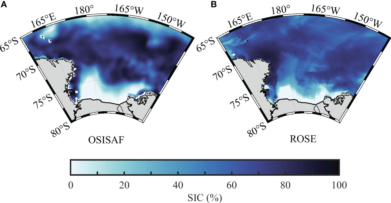
Figure 3 Spatial distributions of the monthly SIC of December 2017 based on (A) OSI SAF and (B) ROSE model results. SIC, sea ice concentration; OSI SAF, Ocean and Sea Ice Satellite Application Facility.

The change in MLD may also influence the near-inertial responses to wind disturbances (e.g., Li et al., 2022). Considering the fact that the MLD has small interannual variability, here we compared the modeled MLD in the year 2017 with the MLD observed by the Apex float (5904150) in the eastern RS shelf in the year 2016 (Porter et al., 2019). Figure 4 shows that the model can reproduce the observed seasonal variation of MLDs with the shallowest and deepest MLDs appearing around January and October, respectively. We note that a more detailed validation of the model results will be presented elsewhere in a separate study.

FIGURE 4

Figure 4 The time series of MLD is simulated by ROSE (blue) and observed by the Apex float 5904150 (red). MLD, mixed layer depth.

3.2 Spatial distribution of NIKE

The spatial distributions of the annual mean surface NIKE and mixed layer-integrated NIKE in the RS are shown in Figures 5A, B, respectively. The spatial distributions of the surface and mixed layer-integrated NIKE resemble each other. Large values are mainly located around the Iselin Bank and the northeastern part of the study area (Figures 5A, B). Both the surface and mixed layer-integrated NIKE have small values near the coast and the ice shelf edge. The background properties of the annual mean wind velocity, SIC, and MLDs are also shown here. Figure 5E shows that the annual mean SIC of the RS is basically greater than 50%. We note that due to the influence of sea ice, the wind power into near-inertial motions was not calculated here. The results of the wind field indicate that southerly winds dominate the RS, with wind speeds of more than 5 m/s occurring mainly in the central and western parts of the RS (Figure 5C).

FIGURE 5

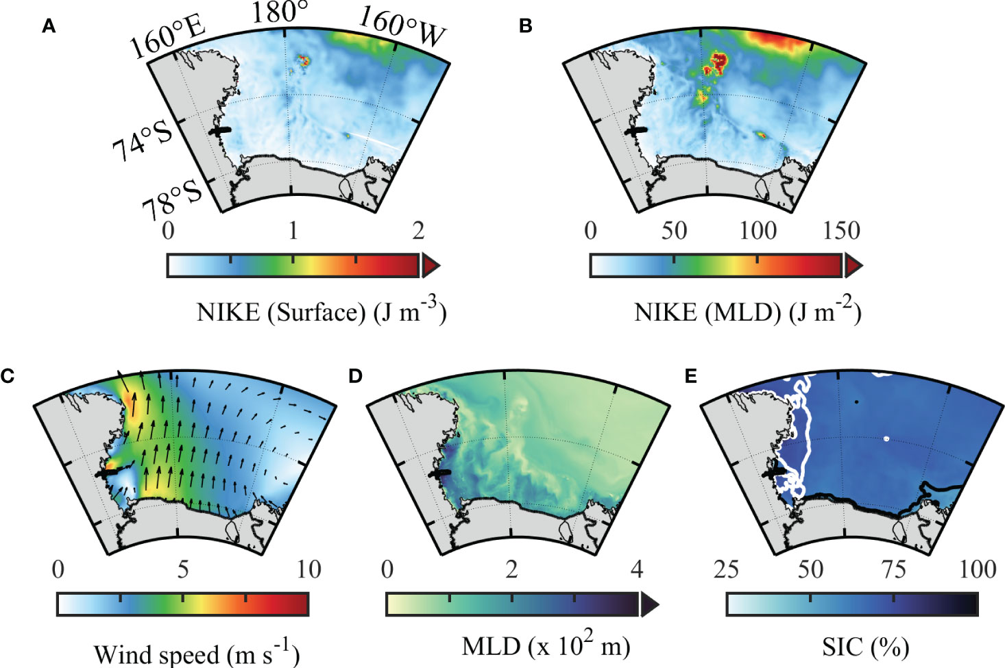
Figure 5 The spatial distribution of the annual mean (A) surface NIKE, (B) mixed layer-integrated NIKE, (C) wind speed and direction, (D) MLD, and (E) SIC. The arrows and colors in (C) represent the wind vectors and wind speed, respectively. The black and white contour lines represent 60% and 70%, respectively. NIKE, near-inertial kinetic energy; MLD, mixed layer depth; SIC, sea ice concentration.

The rotary spectra were next calculated using the baroclinic current velocity at the surface along 175°E during January (Figure 6). Positive and negative frequencies represent counterclockwise and clockwise rotations with time, respectively. The rotary spectra have large values near zero frequency, which indicates the role of geostrophic flow (Elipot and Lumpkin, 2008). In addition to this, another significant spectra peak is located near the local inertial frequency (blue line). The counterclockwise rotation (with time) component contributed most to the variance, consistent with the polarization preference of the NIWs in the Southern Hemisphere. We note that the critical latitude of the semidiurnal tide (~74.5°S for M₂) lies in our study area. The local Coriolis frequency in the RS is close to the frequency of the semidiurnal tide (~1.9323 cpd, cycle per day). This makes that the tidal motions and wind-induced near-inertial motions cannot be distinguished from each other through bandpass filtering in frequency.

FIGURE 6

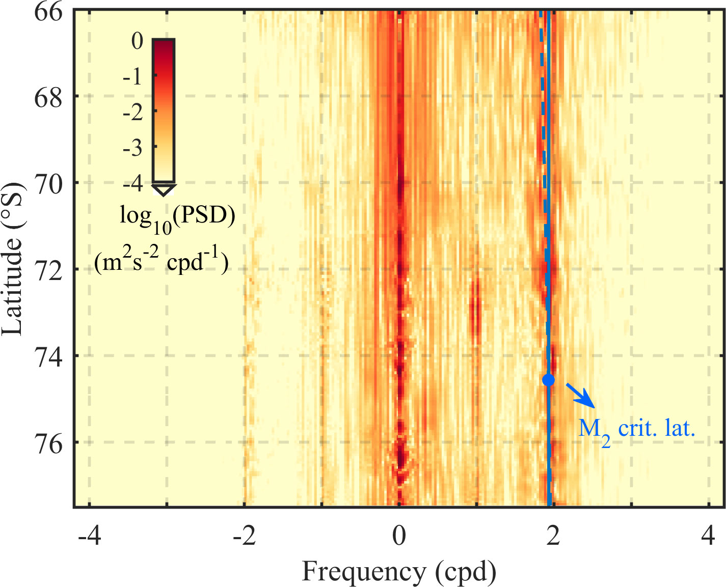
Figure 6 The rotary spectra of the surface current velocity along 175°E in January using a $\text{log}10$ scale in the model. The vertical blue dashed and solid lines represent the local inertial and M₂ tide frequencies, respectively. The latitude where these two lines intersect point is the M₂ critical latitude. PSD, power spectrum density; cpd, cycle per day.

Although the tidal current can contribute to the near-inertial variation at some specific locations (for example, at the Iselin Bank), we suggest that the tidal motions contribute little to the presented NIKE distribution over the RS. The reasons include the following: 1) the tidal current is generally very weak in the RS. Stronger tidal currents are located at the northwestern continental slope of the RS (Robertson, 2005; Padman et al., 2009; Robertson, 2013). Furthermore, the RS is dominated by diurnal tides, which have a much larger amplitude than the semidiurnal tides (Robertson et al., 2003; Robertson, 2005). Figure 6 shows that the near-inertial/semidiurnal bands have a much higher energy level than the diurnal bands. This indicates that the near-inertial peak should not be attributed to the semi-diurnal tides. 2) As we will show later, the NIKE has a strong seasonal variation, which resembles the variation of near-inertial wind stress quite well. 3) Tides are generated by a body force that acts equally on the entire water column, while inertial currents are generated at the surface, which amplifies at the ocean surface. Section 3.4 shows that the near-inertial current is clearly surface-intensified. Furthermore, the wind-driven slab model-simulated and ROSE-simulated surface near-inertial currents agree quite well with each other.

In addition to the above reasons, most importantly, we have run a sensitivity experiment that does not include tidal forcing. The model results directly show that the surface and mixed layer-integrated NIKE with and without tidal forcing resemble each other (for annual mean and monthly surface and mixed layer-integrated NIKE, please see Supplementary Figures 2, 3, respectively). The most apparent NIKE peak appears in the northeast of the study area with similar values. The tidal influence on the near-inertial motion in the upper RS is limited to the regions around Iselin Bank and the continental shelf slope. The wind forcing plays a dominant role in generating near-inertial motions in the upper RS.

3.3 Seasonal variation of NIKE

Figure 7 shows the monthly (January, April, July, and October) surface and mixed layer-integrated NIKE, SIC, and MLDs. Please see Supplementary Figure 4 for the monthly surface NIKE of all 12 months. Both the surface and mixed layer-integrated NIKE show strong seasonal variations with the strongest near-inertial motions observed in April. The surface NIKE has negligible value over the RS in July and October (Figures 7C, D). However, the mixed layer-integrated NIKE in July and October is not that small compared to that in January and April. The MLDs in July and October reach 500 m, which can be an order of magnitude larger than that in January and April. The large surface NIKE in January and April was mainly located in the northeast area off the continental shelf (Figures 7A, B). The large mixed layer-integrated NIKE (>100 J/m²) in January are scattered along the shelf slope and off the RS continental shelf (Figure 7E). This generally coincides with the distribution of surface NIKE.

FIGURE 7

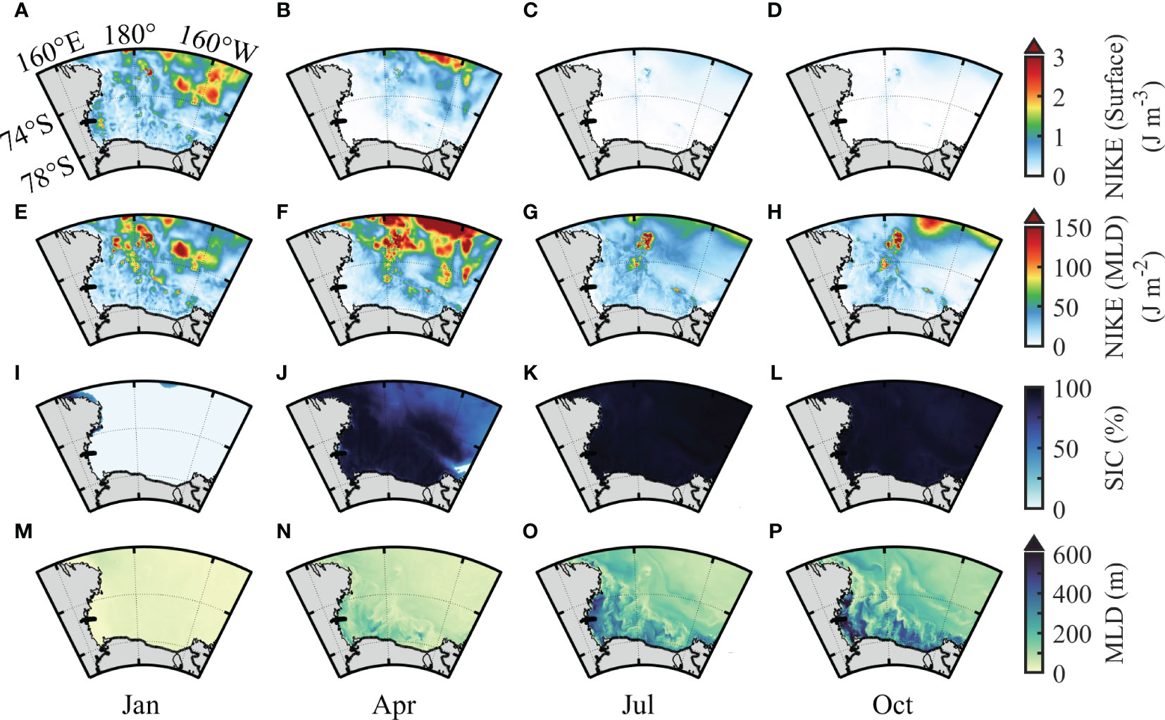
Figure 7 Spatial distribution of the monthly (A–D) surface NIKE, (E–H) mixed layer-integrated NIKE, (I–L) SIC, and (M–P) MLD. The results of four months are shown here: January (A, E, I, M), April (B, F, J, N), July (C, G, K, O), and October (D, H, L, P). NIKE, near-inertial kinetic energy; SIC, sea ice concentration; MLD, mixed layer depth.

In general, strong near-inertial motions were found around the Iselin Bank during all four months. This induced the large annual mean surface and mixed layer-integrated NIKE there (Figures 7A–H). According to the results of the sensitivity test, the constant appearance of strong near-inertial motion around the Iselin Bank during all four months is induced by the local semidiurnal tides.

Sea ice acts as an interface for atmosphere–ocean interactions, which can impede the transport of energy from the atmosphere to the ocean (Rainville and Woodgate, 2009). Previous studies demonstrated that the seasonal variation of sea ice can play an important role in modulating the seasonal variation of NIWs (Rainville and Woodgate, 2009; Guthrie et al., 2013; Martini et al., 2014; Dosser and Rainville, 2016). The RS is of open water in January (Figure 7I). The SIC over the study area increases to >90% in July and October (austral winter and spring). This may account for the low surface NIKE during the same period (Figures 7C, D). The MLD in the RS also shows significant seasonal variability. The potential impact of the different MLDs on the excitation process of NIWs will be discussed in Section 4.1.

3.4 A typical near-inertial response event

Surface winds on the inland shelf of the RS can be influenced by katabatic winds as well as synoptic wind events (Murphy and Simmonds, 1993; Parish and Cassano, 2003). Katabatic winds occur around Victoria Land and Ross Island regions with wind speeds ranging from 10 to 25 m/s (Bromwich, 1991; Parish and Bromwich, 1991; Parish and Cassano, 2003). In addition, frequent cyclone activity affects the surface wind field in the coastal region of the western RS (Cassano and Parish, 2000). These synoptic scale events occur with a frequency of 3–10 days and are characterized by wind speeds of 15–35 m/s (Bromwich, 1991; Parish and Cassano, 2003).

The near-inertial response to a specific strong wind event (~20 m/s) at the RS continental shelf was next examined in detail. The near-inertial bandpass-filtered (0.9 $f_0$–1.15 $f_0$) zonal and meridional velocities at a selected location (Stn. A, 76.5532°S, 170.6250°E, red star in Figure 1) are shown in Figures 8B, C, respectively. The local wind speed at Stn. A increased from 8 to 20 m/s during 10–15 January with a constant southerly wind direction (offshore) (Figure 8A). The near-surface NIWs were effectively excited as a response to this strong wind event (Figures 8B, C). The near-inertial current velocity can reach 10 cm/s (Figures 8B, C). Along the excitation of NIWs, we can also observe the simultaneous change of water temperature, salinity, and MLD. During this strong wind event, the near-surface temperature dropped from ~2°C to −1°C to 0°C (Figure 8D). The near-surface salinity increased from 33.4–33.7 to 34.3–34.5 due to the mixing with salty water in depth (Figure 8E). The MLD deepened from<25 to ~60 m and soon shallowed again after the wind event (black line in Figures 8D–F).

FIGURE 8

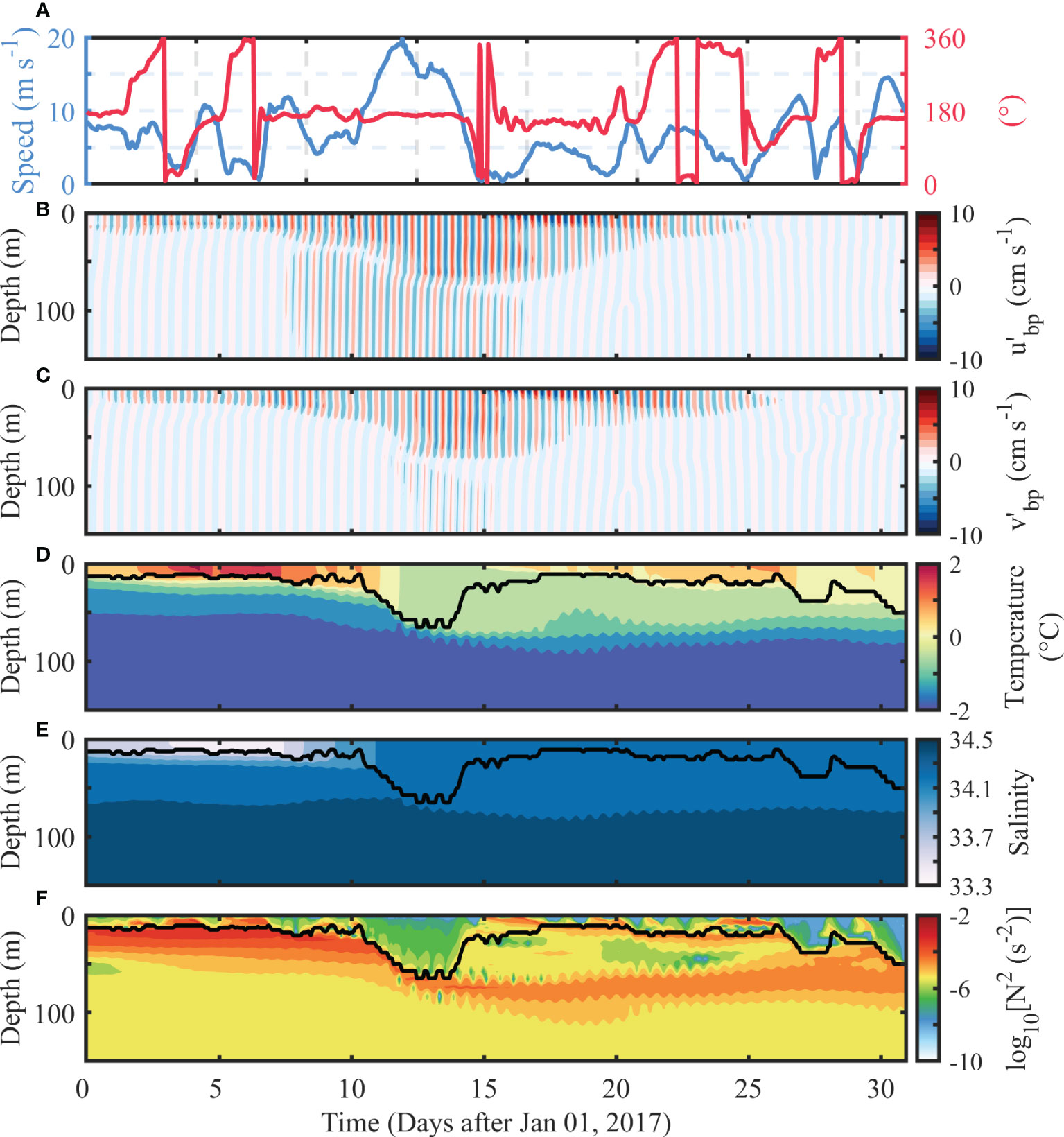
Figure 8 Results of a typical near-inertial response event at Stn. (A) Temporal variations of (A) wind speed and direction. Depth–time maps of near-inertial baroclinic (B) zonal current ($u_{bp}^{\text{'}}$), (C) meridional current ($v_{bp}^{\text{'}}$), (D) temperature, (E) salinity, and (F) squared buoyancy frequency. Black lines in panels (D, E–F) represent the surface MLD. MLD, mixed layer depth.

The evolution of the mixed layer-integrated NIKE maps shows the near-inertial response event more clearly (Figure 9). As a response to the strong wind event, a large NIKE with several cores was excited after 13 January. Stn. A is located at one of the NIKE cores. The NIKE core seems not steady with the position slightly changed. For example, at the beginning of this strong wind event, it seems that the NIKE core near Stn. A moved slightly north–northwest in the following 2–3 days (Figures 9A–D). This may be induced by the advection effect of the background currents on the NIKE. Nevertheless, the oceanic near-inertial responses to the strong wind event are clear.

FIGURE 9

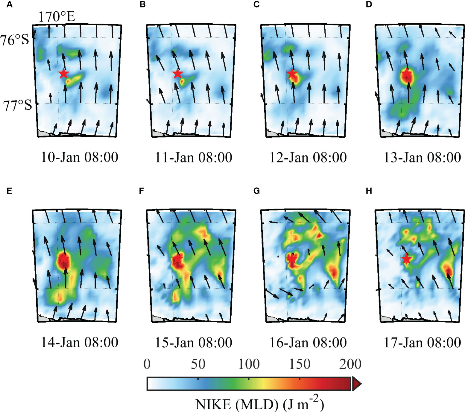
Figure 9 Instantaneous mixed layer-integrated NIKE around Stn. A (red star) from 8:00 A.M. 10 Jan to 17 Jan 2017 (A–H). The red star represents the location as shown in Figure 8. The black arrow represents the wind vectors. NIKE, near-inertial kinetic energy.

To examine the role of wind forcing in exciting the near-inertial currents, we next used the slab model, which was driven by the hourly ERA5 wind dataset. A constant MLD of 20 m was used here for simplification. The slab model predictions were next compared with the ROSE model outputs (Figures 10B, C). Figures 10B, C show that the slab model-simulated mixed layer near-inertial zonal and meridional velocity agrees well with the ROSE outputs in both phase and amplitude. The strong near-inertial response to the wind event is well reproduced. The time-integrated wind-generated near-inertial energy flux grows most rapidly during the wind event with 0.5 KJ/m² NIKE injected into the ocean (Figure 10D). We note that considering the fact that the slab model includes many simplifications such as the constant MLD and the neglect of horizontal propagations of NIWs, the match is fairly good. This demonstrates the dominant role of wind forcing in inducing strong near-inertial responses.

FIGURE 10

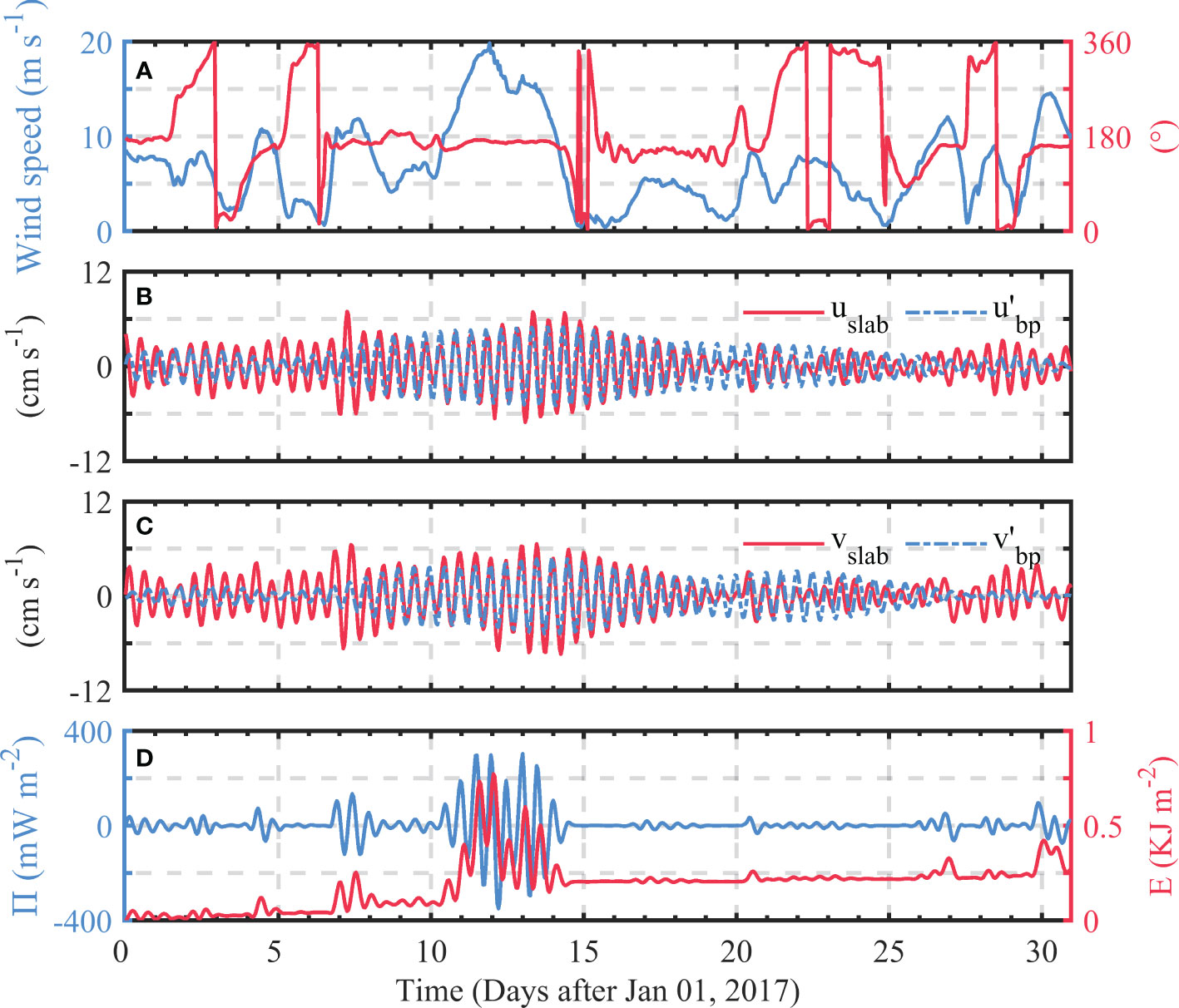
Figure 10 (A) Temporal variation of the wind speed and direction. Comparison of the near-inertial (B) zonal and (C) meridional velocity ($u_{bp}^{\text{'}}$, $v_{bp}^{\text{'}}$) output by the ROSE model with the mixed layer near-inertial zonal and meridional velocity ($u_{slab}$, $v_{slab}$) simulated by the slab model using a constant MLD of 20 m. (D) The wind-generated near-inertial energy flux ($\Pi$) and the time integral of the flux ($E$) estimated based on slab model output. MLD, mixed layer depth.

4 Discussion

4.1 Effect of near-inertial wind stress and mixed layer depth on NIKE distribution

In the linear system, more energy can be injected into the waves with frequencies close to those of the predominant wind stress (Alford et al., 2016; Yang et al., 2019). Therefore, it is conjected that near-inertial wind stress plays a crucial role in producing near-inertial oceanic responses (D'Asaro, 1985; Crawford and Large, 1996; Alford and Whitmont, 2007; Dippe et al., 2015). In addition to the effect of near-inertial wind stress, the sea ice in the polar regions can also influence the near-inertial response, which can impede the transport of energy from the atmosphere to the ocean. The sea ice in the RS has a strong seasonal variation with the open water only occurring in austral summer (Figures 7I–L). To isolate the effect of wind stress on the oceanic near-inertial response in the RS, the austral summer RS is taken as an example of when the wind can act directly on the sea surface.

Figure 11 shows that the spatial distributions of NIWSM and surface NIKE resemble each other. For example, large values are all observed at the northeast of the study area outside the shelf. This demonstrates the dominant role of NIWSM in determining the spatial distribution of NIKE in the austral summer RS. However, we note that there are still some areas of discrepancy between the NIWSM and surface NIKE. For example, large surface NIKE occurs in the western RS continental shelf (74°S–78°S, 162°E–170°E), whereas the NIWSM is weak there (Figures 11B, C).

FIGURE 11

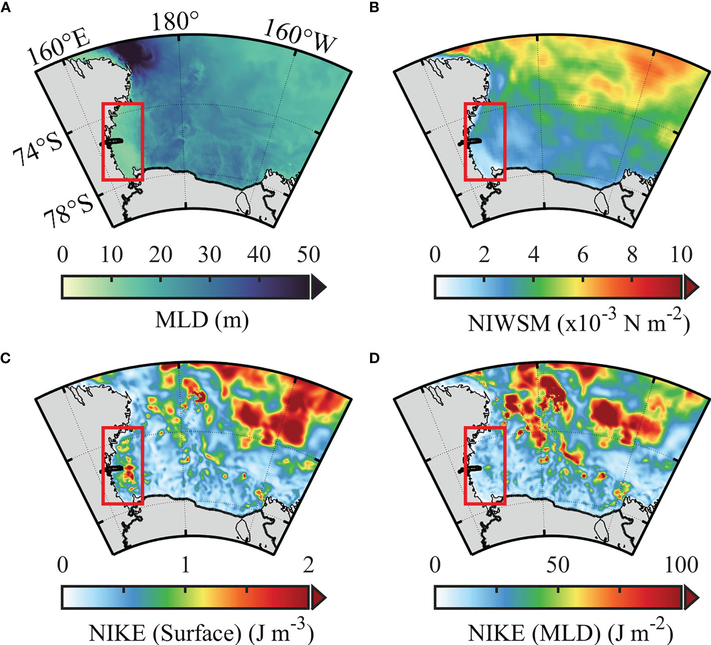
Figure 11 Spatial distribution of the monthly (A) MLD, (B) NIWSM, (C) surface NIKE, and (D) mixed layer-integrated NIKE in January 2017. The red rectangle represents the shallow MLD, and the large surface NIKE area is discussed in the text. NIWSM, near-inertial wave stress magnitude; MLD, mixed layer depth; NIKE, near-inertial kinetic energy.

The mismatch between NIWSM and surface NIKE suggests that there are other factors influencing the distribution of surface NIKE. According to the slab model, Rath et al. (2014) argued that the relationship between surface NIKE and MLD and wind power input (WPI) can be expressed as follows:

$\begin{array}{ll}\frac{\overline{NIKE·}}{\overline{WPI}}=\frac{1}{2ϵH}& (7)\end{array}$

where $\overline{NIKE}$ and $\overline{WPI}$ denote monthly averaged NIKE and monthly averaged WPI, respectively. 1/$ϵ$ is usually considered to be between 2 and 10 days (D'Asaro, 1985). H is the MLD. Dippe et al. (2015) and Rath et al. (2014) both found that NIWSM is a good atmospheric proxy for estimating changes in WPI. From Equation 7, we can expect that the surface NIKE and MLDs are inversely proportional when NIWSM is certain. Therefore, the distribution of surface NIKE must consider the change of MLD.

Figure 11A shows that the MLD in the western RS continental shelf is significantly shallower than in other areas. The surface NIKE there appears to be larger in the areas of shallow MLD. The physical interpretation is that the smaller MLD confines the near-inertial kinetic energy in the thin surface mixed layer, resulting in large values of surface NIKE here. We deform Equation 7 to obtain Equation 8 as below.

$\begin{array}{ll}\frac{\overline{NIKE}·H}{\overline{WPI}}=\frac{1}{2ϵ}& (8)\end{array}$

Equation 8 means that when the spatial variation of the damping time scale is small, the distribution of mixed layer-integrated NIKE is in proportion to the NIWSM. Figure 11D shows that the mixed layer-integrated NIKE has no clear intensification at the west RS, which agrees better with the spatial distribution of NIWSM. Therefore, both the NIWSM and MLD can influence the spatial distribution of NIKE. Specifically, the large surface NIKE outside the continental shelf of the RS is mainly forced by the large NIWSM there, while the surface NIKE peak at the western RS shelf is also influenced by the shallow MLD there.

4.2 Effect of sea ice on NIKE distribution

As discussed above, sea ice plays an important role in the spatial distribution of surface NIKE, as it is the direct interface between the atmosphere and the ocean (Dosser and Rainville, 2016). We next take the results of November and December as an example to demonstrate the potential role of sea ice on NIKE. Figure 12 shows the monthly maps of surface NIKE, mixed layer-integrated NIKE, NIWSM, and SIC in November and December 2017. These two months are characterized by similar wind forcing with the monthly averaged NIWSM during November (2.7 × 10⁻³ N/m²) slightly larger than that during December (2.2 × 10⁻³ N/m²). However, the SIC differs much between these two months, which shows a much lower SIC during December (~41%) than that during November (~71%) (Figures 12G, H). Both the surface and mixed layer-integrated NIKE in December are larger than those in November. This is especially true for the surface NIKE, which has increased approximately 13 times from November to December. Considering the fact that the energy source of NIWs (i.e., the NIWSM) shows little variation between the two months, this indicates that the change of SIC can play an important role in modulating the NIKE in the RS.

FIGURE 12

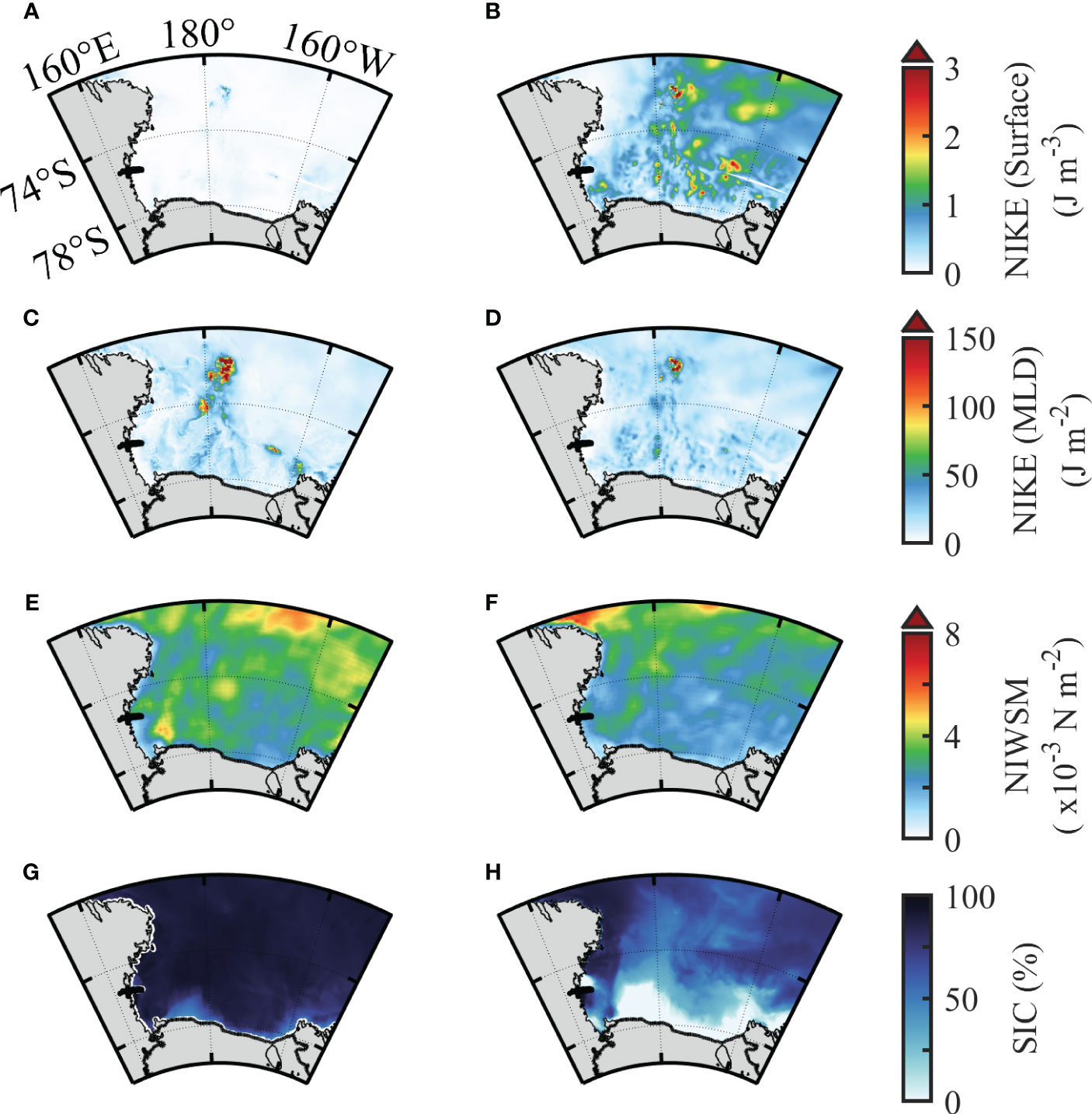
Figure 12 Spatial distribution of the monthly (A, B) surface NIKE, (C, D) mixed layer-integrated NIKE, (E, F) NIWSM, and (G, H) SIC in (A, C, E, G) November and (B, D, F, H) December. NIKE, near-inertial kinetic energy; NIWSM, near-inertial wave stress magnitude; SIC, sea ice concentration.

The monthly SIC, NIWSM, surface NIKE, and mixed layer-integrated NIKE spatially averaged over the RS during 2017 are shown in Figure 13A. The largest surface and mixed layer-integrated NIKE both appear during the austral warm season corresponding to the occurrence of the lowest SIC. Low surface NIKE is found during the remaining months when sea ice presents. The surface NIKE shows a significant negative correlation with the SIC with a correlation coefficient of −0.85 (Figure 13C). Although the seasonal variation of mixed layer-integrated NIKE is influenced by the SIC, it also shows a significant correlation with the NIWSM. If we focus on the time from May to November when the RS is always covered by sea ice, these two parameters show excellent correspondence (Figure 13A). Considering all the 12 months, the correlation coefficient between mixed layer-integrated NIKE and NIWSM reaches 0.40. The low correlation coefficient is mainly due to the presence of another controlling factor, SIC, in driving the seasonal variation of NIKE. For example, the low SIC during the austral summer has induced the largest NIKE even when the NIWSM is just at a mediate level among the 12 months.

FIGURE 13

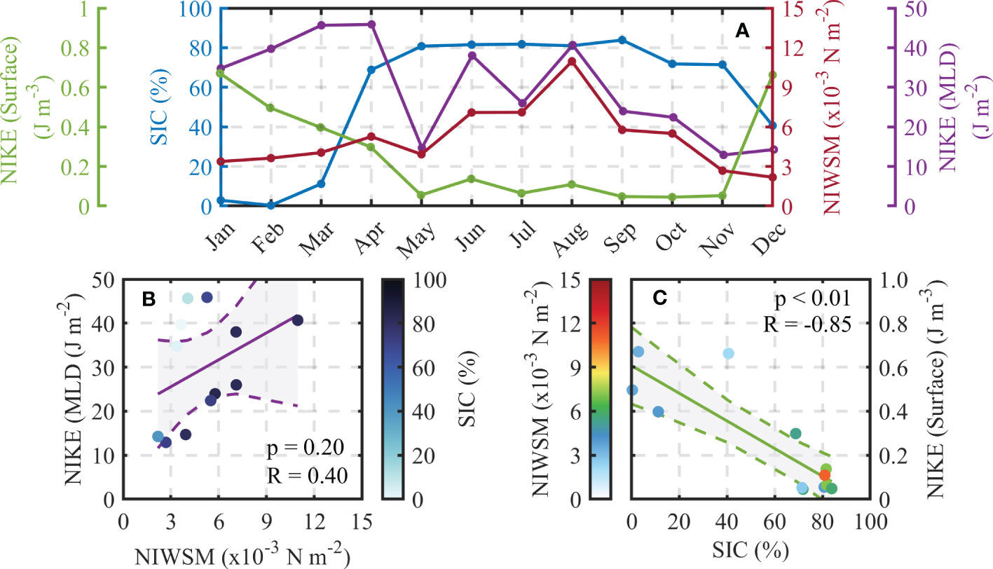
Figure 13 (A) Temporal variation of the monthly SIC (blue), NIWSM (red), surface NIKE (green), and mixed layer-integrated NIKE (purple) spatially averaged in our study area. (B) The scatterplot between the monthly NIWSM and mixed layer-integrated NIKE. The color indicates the corresponding monthly SIC. (C) The scatterplot between the monthly SIC and surface NIKE. The color indicates the monthly NIWSM. The shaded part enclosed by the corresponding dashed line is the 95% confidence interval. SIC, sea ice concentration; NIWSM, near-inertial wave stress magnitude; NIKE, near-inertial kinetic energy.

In addition to the aforementioned influencing factors, previous studies showed that the ratio of the near-inertial energy fluxes radiated to the ocean interior is theoretically proportional to the buoyancy frequency at the mixed layer base (e.g., Voelker et al., 2020). Therefore, the NIKE in the surface mixed layer, which is the radiated NIKE subtracted from the total injected wind energy, should also be related to the buoyancy frequency. However, the calculated results did not find any clear correspondence between the mixed layer-integrated NIKE and the buoyancy frequency at the mixed layer base (figure omitted). This is presumably because the effect of buoyancy frequency is compensated by the change of other influencing factors, such as the near-inertial wind stress. Overall, we summarize that the spatial and temporal variations of NIKE in the RS can, to a large extent, be explained by a combination of the seasonal evolution of NIWSM, SIC, and MLD.

5 Conclusions

This study has focused on the spatial distribution and seasonal variation of NIKE in the upper RS. Based on the high-resolution ROSE model output from January to December 2017 (12 months), we show that the near-inertial component makes a significant contribution to the surface currents in the RS. The semidiurnal tides have a close frequency with the local inertial frequency in the RS. However, the results of the sensitivity experiment without tidal forcing suggest that the tidal contribution to the near-inertial motion in the upper Ross Sea is small, with its influence limited to the regions around Iselin Bank and continental shelf break. The overall near-inertial variability in the upper RS is mainly induced by the change in wind forcing. By looking into the results from a solely wind-forced slab model at an example fixed location on the continental shelf, we show that the slab model-simulated mixed layer near-inertial velocity agrees well with the ROSE outputs, also demonstrating the dominant role of wind forcing in driving the upper ocean near-inertial variability.

The NIWs in the RS show strong temporal and spatial variability. The annual mean surface and mixed layer-integrated NIKE in the upper RS have similar spatial distributions. The NIWSM, which acts as the energy source of NIKE, plays an important role in resulting in the spatial distribution of NIKE. In addition to the peak at the shelf break around Iselin Bank, large surface and mixed layer-integrated NIKE are mainly found in the northeast region outside the continental slope where large near-inertial wind stress occurs. During the ice-free period (austral summer), NIWSM dominates the surface and mixed layer-integrated NIKE distribution off the continental shelf in the RS. The spatial change of MLD can induce spatial discrepancies between surface and mixed layer-integrated NIKE. For example, the shallow MLD in the western RS during January can limit the near-inertial energy in a thin layer, which has induced the large values of surface NIKE there.

The NIKE in the upper RS has a pronounced seasonal cycle with the largest surface and mixed layer-integrated NIKE both observed in austral summer. This is largely due to the fact that the presence of sea ice has impeded the generation of NIWs during the austral winter. The correlation coefficient between monthly averaged surface NIKE and SIC reaches −0.85. During austral summer when sea ice is free, the NIWSM plays a dominant role in determining the spatial distribution of NIKE. The seasonal changes of near-inertial wind stress and SIC both play important roles in regulating the present seasonal cycle of NIKE in the RS.

Data availability statement

The raw data supporting the conclusions of this article will be made available by the authors, without undue reservation.

Author contributions

YMZ processed data, drew pictures, and completed the first draft. WY and HW guided data analysis and the structure of the manuscript. WZ helped to build the ROSE model. YLZ and JS helped with drawing and provided suggestions on the manuscript. All authors contributed to the article and approved the submitted version.

Funding

This study was supported by the National Natural Science Foundation of China (Grant No. 41941008).

Acknowledgments

We would like to thank the organizations that provided the data used in this work, including the European Centre for Medium-Range Weather Forecasts (ECMWF) and the EUMETSAT Ocean and Sea Ice Satellite Application Facility (OSI SAF). We are grateful to the NEMO development team for providing the state-of-the-art model. Finally, we thank the editor and reviewers for their constructive suggestions on our work.

Conflict of interest

The authors declare that the research was conducted in the absence of any commercial or financial relationships that could be construed as a potential conflict of interest.

Publisher’s note

All claims expressed in this article are solely those of the authors and do not necessarily represent those of their affiliated organizations, or those of the publisher, the editors and the reviewers. Any product that may be evaluated in this article, or claim that may be made by its manufacturer, is not guaranteed or endorsed by the publisher.

Supplementary material

The Supplementary Material for this article can be found online at: https://www.frontiersin.org/articles/10.3389/fmars.2023.1173900/full#supplementary-material

References

Alford M. H. (2003). Improved global maps and 54-year history of wind-work on ocean inertial motions. Geophys. Res. Lett. 30 (8), 1424. doi: 10.1029/2002gl016614

CrossRef Full Text | Google Scholar

Alford M. H. (2020). Global calculations of local and remote near-inertial-wave dissipation. J. Phys. Oceanogr. 50 (11), 3157–3164. doi: 10.1175/JPO-D-20-0106.1

CrossRef Full Text | Google Scholar

Alford M. H., MacKinnon J. A., Simmons H. L., Nash J. D. (2016). Near-inertial internal gravity waves in the ocean. Annu. Rev. Mar. Sci. 8 (1), 95–123. doi: 10.1146/annurev-marine-010814-015746

CrossRef Full Text | Google Scholar

Alford M. H., Whitmont M. (2007). Seasonal and spatial variability of near-inertial kinetic energy from historical moored velocity records. J. Phys. Oceanogr. 37 (8), 2022–2037. doi: 10.1175/JPO3106.1

CrossRef Full Text | Google Scholar

Bromwich D. H. (1991). Mesoscale cyclogenesis over the southwestern Ross Sea linked to strong katabatic winds. Monthly Weather Rev. 119 (7), 1736–1753. doi: 10.1175/1520-0493(1991)119<1736:MCOTSR>2.0.CO;2

CrossRef Full Text | Google Scholar

Cassano J. J., Parish T. R. (2000). An analysis of the nonhydrostatic dynamics in numerically simulated Antarctic katabatic flows. J. Atmospheric Sci. 57 (6), 891–898. doi: 10.1175/1520-0469(2000)057<0891:AAOTND>2.0.CO;2

CrossRef Full Text | Google Scholar

Comiso J. C., Kwok R., Martin S., Gordon A. L. (2011). Variability and trends in sea ice extent and ice production in the Ross Sea. J. Geophys. Res.: Oceans 116 (C4), C04021. doi: 10.1029/2010JC006391

CrossRef Full Text | Google Scholar

Crawford G., Large W. (1996). A numerical investigation of resonant inertial response of the ocean to wind forcing. J. Phys. Oceanogr. 26 (6), 873–891. doi: 10.1175/1520-0485(1996)026<0873:ANIORI>2.0.CO;2

CrossRef Full Text | Google Scholar

D'Asaro E. A. (1985). The energy flux from the wind to near-inertial motions in the surface mixed layer. J. Phys. Oceanogr. 15 (8), 1043–1059. doi: 10.1175/1520-0485(1985)015<1043:TEFFTW>2.0.CO;2

CrossRef Full Text | Google Scholar

D'Asaro E. A., Eriksen C. C., Levine M. D., Niiler P., Van Meurs P. (1995). Upper-ocean inertial currents forced by a strong storm. part I: data and comparisons with linear theory. J. Phys. Oceanogr. 25 (11), 2909–2936. doi: 10.1175/1520-0485(1995)025<2909:UOICFB>2.0.CO;2

CrossRef Full Text | Google Scholar

de Boyer Montégut C., Madec G., Fischer A. S., Lazar A., Iudicone D. (2004). Mixed layer depth over the global ocean: an examination of profile data and a profile-based climatology. J. Geophys. Res.: Oceans 109 (C12), C12003. doi: 10.1029/2004JC002378

CrossRef Full Text | Google Scholar

Dippe T., Zhai X., Greatbatch R. J., Rath W. (2015). Interannual variability of wind power input to near-inertial motions in the north Atlantic. Ocean Dyn. 65 (6), 859–875. doi: 10.1007/s10236-015-0834-x

CrossRef Full Text | Google Scholar

Dosser H. V., Rainville L. (2016). Dynamics of the changing near-inertial internal wave field in the Arctic ocean. J. Phys. Oceanogr. 46 (2), 395–415. doi: 10.1175/jpo-d-15-0056.1

CrossRef Full Text | Google Scholar

Elipot S., Lumpkin R. (2008). Spectral description of oceanic near-surface variability. Geophys. Res. Lett. 35 (5), L05606. doi: 10.1029/2007GL032874

CrossRef Full Text | Google Scholar

Ferrari R., Wunsch C. (2009). Ocean circulation kinetic energy: reservoirs, sources, and sinks. Annu. Rev. Fluid Mechanics 41 (1), 253–282. doi: 10.1146/annurev.fluid.40.111406.102139

CrossRef Full Text | Google Scholar

Firing E., Lien R. C., Muller P. (1997). Observations of strong inertial oscillations after the passage of tropical cyclone ofa. J. Geophys. Res.: Oceans 102 (C2), 3317–3322. doi: 10.1029/96JC03497

CrossRef Full Text | Google Scholar

Garrett C. (2001). What is the “near-inertial” band and why is it different from the rest of the internal wave spectrum? J. Phys. Oceanogr. 31 (4), 962–971. doi: 10.1175/1520-0485(2001)031<0962:WITNIB>2.0.CO;2

CrossRef Full Text | Google Scholar

Gerringa L. J. A., Alderkamp A.-C., van Dijken G., Laan P., Middag R., Arrigo K. R. (2020). Dissolved trace metals in the Ross Sea. Front. Mar. Sci. 7. doi: 10.3389/fmars.2020.577098

CrossRef Full Text | Google Scholar

Gordon A. L., Padman L., Bergamasco A. (2009). Southern ocean shelf slope exchange. Deep Sea Res. Part II Topical Stud. Oceanogr. 56 (13-14), 775–777. doi: 10.1016/j.dsr2.2008.11.002

CrossRef Full Text | Google Scholar

Guan S., Zhao W., Huthnance J., Tian J., Wang J. (2014). Observed upper ocean response to typhoon megi, (2010) in the northern south China Sea. J. Geophys. Res.: Oceans 119 (5), 3134–3157. doi: 10.1002/2013jc009661

CrossRef Full Text | Google Scholar

Guthrie J. D., Morison J. H. (2021). Not just Sea ice: other factors important to near-inertial wave generation in the Arctic ocean. Geophys. Res. Lett. 48 (3), e2020GL090508. doi: 10.1029/2020gl090508

CrossRef Full Text | Google Scholar

Guthrie J. D., Morison J. H., Fer I. (2013). Revisiting internal waves and mixing in the Arctic ocean. J. Geophys. Res.: Oceans 118 (8), 3966–3977. doi: 10.1002/jgrc.20294

CrossRef Full Text | Google Scholar

Hebert D., Moum J. (1994). Decay of a near-inertial wave. J. Phys. Oceanogr. 24 (11), 2334–2351. doi: 10.1175/1520-0485(1994)024<2334:DOANIW>2.0.CO;2

CrossRef Full Text | Google Scholar

Holland P. R., Kwok R. (2012). Wind-driven trends in Antarctic sea-ice drift. Nat. Geosci. 5 (12), 872–875. doi: 10.1038/ngeo1627

CrossRef Full Text | Google Scholar

Hummels R., Dengler M., Rath W., Foltz G. R., Schutte F., Fischer T., et al. (2020). Surface cooling caused by rare but intense near-inertial wave induced mixing in the tropical Atlantic. Nat. Communication 11 (1), 3829. doi: 10.1038/s41467-020-17601-x

CrossRef Full Text | Google Scholar

Jiang J., Lu Y., Perrie W. (2005). Estimating the energy flux from the wind to ocean inertial motions: the sensitivity to surface wind fields. Geophys. Res. Lett. 32 (15), L15610. doi: 10.1029/2005GL023289

CrossRef Full Text | Google Scholar

Li J., Zhai X., Liu J., Yan T., He Y., Chen Z., et al. (2022). Spatial and seasonal variations of near-inertial kinetic energy in the upper south China Sea: role of synoptic atmospheric systems. Prog. Oceanogr. 208 (1), 102899. doi: 10.1016/j.pocean.2022.102899

CrossRef Full Text | Google Scholar

Lu H., Chen Z., Xu K., Liu Z., Wang C., Xu J., et al. (2022). Interannual variability of near-inertial energy in the south China Sea and Western north pacific. Geophys. Res. Lett. 49 (24), e2022GL100984. doi: 10.1029/2022GL100984

CrossRef Full Text | Google Scholar

Martini K. I., Simmons H. L., Stoudt C. A., Hutchings J. K. (2014). Near-inertial internal waves and Sea ice in the Beaufort Sea. J. Phys. Oceanogr. 44 (8), 2212–2234. doi: 10.1175/jpo-d-13-0160.1

CrossRef Full Text | Google Scholar

Munk W., Wunsch C. (1998). Abyssal recipes II: energetics of tidal and wind mixing. Deep Sea Res. Part I: Oceanogr. Res. Papers 45 (12), 1977–2010. doi: 10.1016/S0967-0637(98)00070-3

CrossRef Full Text | Google Scholar

Murphy B. F., Simmonds I. (1993). An analysis of strong wind events simulated in a GCM near Casey in the Antarctic. Monthly Weather Rev. 121 (2), 522–534. doi: 10.1175/1520-0493(1993)121<0522:AAOSWE>2.0.CO;2

CrossRef Full Text | Google Scholar

Oey L.-Y., Ezer T., Wang D.-P., Fan S.-J., Yin X.-Q. (2006). Loop current warming by hurricane Wilma. Geophys. Res. Lett. 33 (8), L08613. doi: 10.1029/2006GL025873

CrossRef Full Text | Google Scholar

Orsi A. H., Johnson G. C., Bullister J. L. (1999). Circulation, mixing, and production of Antarctic bottom water. Prog. Oceanogr. 43 (1), 55–109. doi: 10.1016/S0079-6611(99)00004-X

CrossRef Full Text | Google Scholar

Orsi A. H., Wiederwohl C. L. (2009). A recount of Ross Sea waters. Deep Sea Res. Part II 56 (13-14), 778–795. doi: 10.1016/j.dsr2.2008.10.033

CrossRef Full Text | Google Scholar

Padman L., Howard S. L., Orsi A. H., Muench R. D. (2009). Tides of the northwestern Ross Sea and their impact on dense outflows of Antarctic bottom water. Deep Sea Res. Part II: Topical Stud. Oceanogr. 56 (13-14), 818–834. doi: 10.1016/j.dsr2.2008.10.026

CrossRef Full Text | Google Scholar

Parish T. R., Bromwich D. H. (1991). Continental-scale simulation of the Antarctic katabatic wind regime. J. Climate 4 (2), 135–146. doi: 10.1175/1520-0442(1991)004<0135:CSSOTA>2.0.CO;2

CrossRef Full Text | Google Scholar

Parish T. R., Cassano J. J. (2003). The role of katabatic winds on the Antarctic surface wind regime. Monthly Weather Rev. 131 (2), 317–333. doi: 10.1175/1520-0493(2003)131<0317:TROKWO>2.0.CO;2

CrossRef Full Text | Google Scholar

Parkinson C. L. (2002). Trends in the length of the southern ocean sea-ice season. Ann. Glaciol. 34, 435–440. doi: 10.3189/172756402781817482

CrossRef Full Text | Google Scholar

Pollard R. T. (1980). Properties of near-surface inertial oscillations. J. Phys. Oceanogr. 10 (3), 385–398. doi: 10.1175/1520-0485(1980)010<0385:Ponsio>2.0.Co;2

CrossRef Full Text | Google Scholar

Pollard R. T., Millard R. C. (1970). Comparison between observed and simulated wind-generated inertial oscillations. Deep Sea Res. Oceanogr. Abst. 17 (4), 813–821. doi: 10.1016/0011-7471(70)90043-4

CrossRef Full Text | Google Scholar

Porter D. F., Springer S. R., Padman L., Fricker H. A., Tinto K. J., Riser S. C., et al. (2019). Evolution of the seasonal surface mixed layer of the Ross Sea, Antarctica, observed with autonomous profiling floats. J. Geophys. Res.: Oceans 124 (7), 4934–4953. doi: 10.1029/2018jc014683

CrossRef Full Text | Google Scholar

Price J. F. (1981). Upper ocean response to a hurricane. J. Phys. Oceanogr. 11 (2), 153–175. doi: 10.1175/1520-0485(1981)011<0153:UORTAH>2.0.CO;2

CrossRef Full Text | Google Scholar

Rainville L., Lee C., Woodgate R. (2011). Impact of wind-driven mixing in the Arctic ocean. Oceanography 24 (3), 136–145. doi: 10.5670/oceanog.2011.65

CrossRef Full Text | Google Scholar

Rainville L., Woodgate R. A. (2009). Observations of internal wave generation in the seasonally ice-free Arctic. Geophys. Res. Lett. 36 (23), L23604. doi: 10.1029/2009gl041291

CrossRef Full Text | Google Scholar

Rath W., Greatbatch R. J., Zhai X. (2014). On the spatial and temporal distribution of near-inertial energy in the southern ocean. J. Geophys. Res.: Oceans 119 (1), 359–376. doi: 10.1002/2013jc009246

CrossRef Full Text | Google Scholar

Robertson R. (2005). Baroclinic and barotropic tides in the Ross Sea. Antarctic Sci. 17 (1), 107–120. doi: 10.1017/s0954102005002506

CrossRef Full Text | Google Scholar

Robertson R. (2013). Tidally induced increases in melting of amundsen Sea ice shelves. J. Geophys. Res.: Oceans 118 (6), 3138–3145. doi: 10.1002/jgrc.20236

CrossRef Full Text | Google Scholar

Robertson R., Beckmann A., Hellmer H. (2003). M2 tidal dynamics in the Ross Sea. Antarctic Sci. 15 (1), 41–46. doi: 10.1017/S0954102003001044

CrossRef Full Text | Google Scholar

Shay L. K., Mariano A. J., Jacob S. D., Ryan E. H. (1998). Mean and near-inertial ocean current response to hurricane Gilbert. J. Phys. Oceanogr. 28 (5), 858–889. doi: 10.1175/1520-0485(1998)028<0858:MANIOC>2.0.CO;2

CrossRef Full Text | Google Scholar

Silverthorne K. E., Toole J. M. (2009). Seasonal kinetic energy variability of near-inertial motions. J. Phys. Oceanogr. 39 (4), 1035–1049. doi: 10.1175/2008JPO3920.1

CrossRef Full Text | Google Scholar

Smith W., Sedwick P., Arrigo K., Ainley D., Orsi A. (2012). The Ross Sea in a Sea of change. Oceanography 25 (3), 90–103. doi: 10.5670/oceanog.2012.80

CrossRef Full Text | Google Scholar

Song H., Marshall J., Campin J. M., McGillicuddy D. J. (2019). Impact of near-inertial waves on vertical mixing and air-sea CO₂ fluxes in the southern ocean. J. Geophys. Res.: Oceans 124 (7), 4605–4617. doi: 10.1029/2018jc014928

CrossRef Full Text | Google Scholar

Subeesh M., Ravichandran M., Chatterjee S., Pramanik A., Nuncio M. (2022). Near-inertial waves in an Arctic fjord and their impact on vertical mixing of Atlantic water mass. Prog. Oceanogr. 206, 102844. doi: 10.1016/j.pocean.2022.102844

CrossRef Full Text | Google Scholar

Voelker G. S., Olbers D., Walter M., Mertens C., Myers P. G. (2020). Estimates of wind power and radiative near-inertial internal wave flux: The hybrid slab model and its application to the North Atlantic. Ocean Dynamics 70(11), 1357–1376. doi: 10.1007/s10236-020-01388-y

PubMed Abstract | CrossRef Full Text | Google Scholar

Watanabe M., Hibiya T. (2002). Global estimates of the wind-induced energy flux to inertial motions in the surface mixed layer. Geophys. Res. Lett. 29 (8), 1239. doi: 10.1029/2001GL014422

CrossRef Full Text | Google Scholar

Yang W., Hibiya T., Tanaka Y., Zhao L., Wei H. (2019). Diagnostics and energetics of the topographic rossby waves generated by a typhoon propagating over the ocean with a continental shelf slope. J. Oceanogr. 75 (6), 503–512. doi: 10.1007/s10872-019-00518-5

CrossRef Full Text | Google Scholar

Yang W., Wei H., Liu Z., Li G. (2021). Intermittent intense thermocline shear associated with wind-forced near-inertial internal waves in a summer stratified temperate shelf Sea. J. Geophys. Res.: Oceans 126 (12), e2021JC017576. doi: 10.1029/2021jc017576

CrossRef Full Text | Google Scholar

Yang W., Wei H., Liu Z., Zhao L. (2023). Widespread intensified pycnocline turbulence in the summer stratified yellow Sea. J. Geophys. Res.: Oceans 128 (1), e2022JC019023. doi: 10.1029/2022jc019023

CrossRef Full Text | Google Scholar

Yu X., Naveira Garabato A. C., Vic C., Gula J., Savage A. C., Wang J., et al. (2022). Observed equatorward propagation and chimney effect of near-inertial waves in the midlatitude ocean. Geophys. Res. Lett. 49 (13), e2022GL098522. doi: 10.1029/2022GL098522

CrossRef Full Text | Google Scholar