Relative importance of ENSO and IOD on interannual variability of Indonesian Throughflow transport

1 Introduction

The Indonesian Throughflow (ITF) originates from the western Pacific Ocean, and then passes through the Indonesian Sea to enter the Indian Ocean. The ITF carries a large amount of warmer and fresher waters with an annual average volume transport of approximately 15 Sv (1 Sv=10⁶ m³ s^-1) (Wijffels et al., 2008; Sprintall et al., 2009; Gordon et al., 2010; Susanto et al., 2012; Liu et al., 2015; Sprintall et al., 2019), and heat transport of 0.24–1.15 PW (1 PW = 10¹⁵ W) from the Pacific to the Indian Ocean (Hirst and Godfrey, 1993; Vranes et al., 2002; Tillinger and Gordon, 2009; Xie et al., 2019; Zhang et al., 2019). It has a significant impact on the thermohaline structure and velocity profiles flowing through the oceans (Lee et al., 2019; Pang et al., 2022). This provides an important low-latitude ocean channel for the transmission of climate signals and anomalies in the global thermohaline circulation. The ITF regulates the local atmosphere system by influencing air-sea exchange and precipitation at different time scales, which in turn has a far-reaching effect on the global climate (Gordon, 1986; Godfrey, 1996; Gordon, 2005; Sprintall et al., 2014; Hu et al., 2019; Yuan et al., 2022). Thus, the variability of ITF transport has to be understood to interpret climate change.

The ITF transport is not well determined observationally due to several inflow and outflow channels, such as the Makassar Strait, Maluku Strait, Halmahera Strait, Lombok Strait, Ombai Strait, and Timor Strait. Among them, the Makassar Strait accounts for approximately 77% of the ITF transport and is thus considered the main inflow channel of the ITF (Du and Qu, 2010; Gordon et al., 2010; Gordon et al., 2019). Therefore, several international observation programs have been conducted there to detect the changes in ITF transport, such as the Arlindo Mixing program, the International Nusantara Stratification and Transport program (INSTANT), and the Monitoring the ITF program (MITF). The long-term mooring data of the Makassar Strait reveals that the average thermocline (0–300 m) southward transport (9.1 Sv) contributed about 73% of the total transport (12.5 Sv) (Gordon et al., 2019). In addition to the mooring observation data, temperature data measured by repeated expendable bathythermograph (XBT) and Argo buoy data of IX1 section were also used to deduce the geostrophic current transport of the ITF (Wijffels et al., 2008; Liu et al., 2015). Based on 30 years of XBT data – from 1984 to 2013 ITF geostrophic transport experienced a strengthening trend of ~0.1 Sv year^-1 (Liu et al., 2015). In addition, numerous numerical models and reanalysis data demonstrate a relatively consistent interannual variability with the observed data (Masumoto et al., 2004; Feng et al., 2013; Yuan et al., 2013).

The ITF variability is mainly driven by large scale sea level gradients between the Pacific and Indian Ocean basins (Wyrtki, 1987). Specifically, the sea surface height (SSH) difference between the northwest tropical Pacific (NWP) and the southeast Indian Ocean (SEI) is a favorable indicator of ITF transport, which is largely dominated by the El Niño-Southern Oscillation (ENSO) and the Indian Ocean Dipole (IOD), respectively. The ITF is generally strong (weak) during La Niña (El Niño) events (Meyers, 1996). This is because the Pacific trade winds and the Walker circulation strengthening (weakening), which leads to an increase (decrease) of sea level in the western Pacific (Meyers, 1996; Gordon et al., 1999; Sprintall and Révelard, 2014; Hu and Sprintall, 2016). During negative (positive) IOD events, when the eastern and western surface water of the tropical Indian Ocean appear abnormally warm (cold) and cold (warm), downwelling (upwelling) occurs in the eastern sea surface of the tropical eastern Indian Ocean. This favors a positive (negative) sea level anomaly in that region and thus suppresses (strengths) the ITF (Cai et al., 2011; Yuan et al., 2011). Increasing number of studies show that IOD events have a more significant impact on the ITF (Sprintall et al., 2009; Sprintall and Révelard, 2014; Liu et al., 2015; Pujiana et al., 2019). However, ENSO and IOD events often occur concurrently (Murtugudde et al., 1998; Saji et al., 1999; Feng et al., 2001), and hence, it is hard to tease out the individual effects of each climate mode on ITF variability. Quantitative analysis of the influences of ENSO and IOD on ITF changes are not yet well clarified.

In this study, four high-resolution reanalysis datasets are used to detect the spatial-temporal variability of the ITF inflow and outflow. A machine learning method is adopted to express whether the ENSO or the IOD is the dominant climate driver for the ITF variability during different periods. The study is explained as follows. The four reanalysis datasets and the methods are depicted in section 2. The temporal and spatial changes of ITF transport are explained in section 3. The dominant climate indices affecting the ITF in different periods are studied in section 4. The possible mechanisms are discussed in section 5, and the conclusions are given in section 6.

2 Data and methods

2.1 Mooring data

Mooring data are obtained from three straits: the Makassar Strait, Ombai Strait, and Timor Strait. Among them, the Makassar mooring data is procured from the INSTANT and MITF observation projects, whereas the Ombai and Timor are from the Integrated Marine Observing System (IMOS, 2022).

2.1.1 INSTANT

In January 2004, two moorings were deployed in the Labani channel in the Makassar Strait as part of an international program to monitor the major ITF inflow routes: 2°51.9′S, 118°27.3′E, and 2°51.5′S, 118°37.7′E (Gordon et al., 2008; Gordon et al., 2010). In July 2005 and November 27, 2006, the moorings were repeatedly recovered and redeployed. The moorings measured the three-dimensional velocity components at 30 min intervals.

2.1.2 MITF

Only one mooring was deployed at 2°51.9′S, 118°27.3′E as part of the MITF program on 22 November 2006, after the INSTANT project. MITF was designed to receive data and was redeployed every two years. Due to equipment transportation problems, there are no data from August 2011 to August 2013. At the mooring location, upward-looking and downward-looking acoustic Doppler current profilers (ADCPs) were placed at 463 m and 487 m to record flow data for the entire channel at a depth of 680 m. The positions varied slightly throughout the observation period but remained roughly the same. In August 2015, two ADCPs were placed at the same buoy station at 498 m, and two χ‐pods (small autonomous instruments), which can measure the temperature gradient spectrum using a fast thermistor, were placed at the same position to measure the temperature microstructure (Gordon et al., 2019). The MITF data up to August 2017 is used in this study, though the project is still ongoing.

2.1.3 IMOS

The IMOS has moorings across both its National Mooring Network and Deep Water Moorings facilities. This system provides parameters such as temperature, salinity, dissolved oxygen, chlorophyll estimates, turbidity, down-welling photosynthetic photon flux (PAR), and current velocity, accompanied by depth and pressure when available. The observations were made using a range of temperature loggers, conductivity-temperature-depth (CTD) instruments, water-quality monitors (WQM), ADCPs, and single-point current meters. In this study, we use the single-point mooring data (OMB) for the Ombai Strait at 125.08°E, 8.52°S, which ranges from June 19, 2011, to October 21, 2015. For the Timor Strait, we mainly use three mooring data: Timor North (TNorth), Timor North Slope (TNSlope), and Timor South (TSouth), which cover from June 14, 2011 to April 15, 2014. These are the hourly mooring data, and the vertical depth reaches 520.95m.

2.2 Reanalysis data

Four reanalysis datasets are used: Copernicus Marine Environment Monitoring Service (CMEMS), OGCM For Earth Simulator (OFES), Hybrid Coordinate Ocean Model (HYCOM), and simple Ocean Data Assimilation Ocean/Sea Ice Reanalysis (SODA), respectively.

2.2.1 CMEMS

For the CMEMS, the version GLOBAL_MULTIYEAR_PHY_001_030 global reanalysis data with a monthly average from 1993 to 2019 is used. The data have a spatial resolution of 1/12° × 1/12° (about 8 km × 8 km at the equator) and a total of 50 standard layers in the vertical direction. The reanalysis data assimilate many available observations. The time range is from 1993 to 2020, which covers the most recent period of altimeter data (beginning with the launch of TOPEX/Poseidon and ERS-1 satellites in the early 1990s).

2.2.2 OFES

OFES data is a global 0.1° × 0.1° × 54 layers model data forced by NCEP winds. The output is an integration of more than 50 years. The OFES data used is the monthly average from 1993 to 2017.

2.2.3 HYCOM

The HYCOM versions of GLBu0.08/expt_19.0, GLBu0.08/expt_90.9, and GLBv0.08/expt_93.0 cover the time range 1993–2012, 2013–2017 and 2018–2019, respectively. The global 0.08° × 0.08° horizontal resolution and 40 vertical resolution of depth levels are daily reanalysis data from 1993 to 2019.

2.2.4 SODA

SODA is a reanalysis data set that covers the global ocean (except some polar sea areas) jointly developed by the University of Maryland and Texas A&M University. The latest version, SODA 3.4.2, which adopts the Modular Ocean Model (MOM5) of 0.5° × 0.5° × 50 layers (horizontal spacing at the equator 28 km, polar location less than 10 km) is used in this study. The time range of the monthly reanalysis data is from 1993 to 2019.

2.3 Methods

2.3.1 Transport calculation

Many methods are used to calculate the flow in channels, including the volume flux (Anderson et al., 1986) and the P-vector methods (Chu, 1995). The volume flux method is used to take full advantage of the high-resolution datasets:

$\begin{array}{ll}{F}_v={\displaystyle \sum _{k=1}^{nz}{\displaystyle \sum _{i=1}^{ns}\overrightarrow{v_{ik}}·d{x}_i·d{z}_k.}}& (1)\end{array}$

Among them, $\overrightarrow{v_{i,k}}$ is perpendicular to the $i$ th horizontal grid and the $k$ th vertical grid on the cross-section flow velocity, $i$ is the location of the cross-section grid point number, $ns$ is the number of grid points, $x_i$ is the distance between two adjacent grid points, $k$ is the number of vertical layers, $nz$ is the number of vertical layers, and $d{z}_k$ is the distance between two adjacent vertical layers.

2.3.2 Removal of potential dependency between climate drivers

ENSO and the IOD events often occur synchronously; hence, they can interact with each other. Therefore, linear regression is used to eliminate the possible influence of Niño 3.4 on IOD (Saji and Yamagata, 2003), as follows:

$\begin{array}{ll}\widehat{DMI}=a\times Nino 3.4+b,& (2)\end{array}$

$\begin{array}{ll}DM{I}_{new}=DMI-\widehat{DMI}.& (3)\end{array}$

where $\widehat{DMI}$ represents the linear fitting term of $Nino3.4$, $a$ and $b$ represent the trend and offset, respectively, and $DM{I}_{new}$ indicates the new DMI, excluding the $Nino3.4$ trend item.

2.3.3 Random Forest model

A machine learning decision method, named Random Forest (RF) is employed to determine the contribution of climate drivers to the interannual variation of the ITF. RF is a kind of ensemble learning algorithm. The general idea of RF is to train multiple weak models to pack together to form a strong model. The performance of the strong model is much better than that of a single weak model. Hence, the results of the multi-models have higher accuracy and generalization performance.

Unlike the simple linear correlation and regression methods, RF methods can be used to study complex relationships between variables and can reveal nonlinear and hierarchical relationships between responses and predictors (Feng et al., 2022). RF builds the model by combining predictors and evaluates the relative importance of each predictor. In this study, an out-of-bag (OOB) generated accuracy-based materiality measure is used. When building the model, approximately one-third of the relevant data was randomly selected for model verification. When variables in the OOB samples are randomly disturbed, the average prediction accuracy is defined as the important value of the corresponding variable (Heung et al., 2014), which is expressed as the mean square error:

$\begin{array}{ll}MS{E}_{OOB}=\frac{1}{N}{\displaystyle \sum _{K=1}^N{(O_i-P_{KOOB})}^2.}& (4)\end{array}$

where $N$ is the number of observations, $O_i$ represents actual data and $P_{KOOB}$ indicates the average of all OOB predictions across all trees.

3 Variability of ITF

Mooring observation in the Makassar Strait reveals different water masses in the upper (0–300 m) and lower (300–760 m) layers, respectively. The ITF is separated into the upper and lower parts, with a depth boundary of 300 m, to reveal the impacts of climate modes on the vertical structures. To facilitate later research, the 0–300 m layer is defined as the upper layer and the 300–760 m layer as the lower layer. Due to the depth limitation of the Ombai and Timor Straits, the lower layer is 300–520 m. In accordance with Li et al. (2020), the inflow is defined as that the sections of Sulawesi Sea (125°E, 1°N–6°N), Maluku Sea (125°E–127.5°E, 0.5°N), and Halmahera Sea (128°E–131°E, 0.5°S), respectively, and the outflow is defined as that across the eastern tropical Indian Ocean section (114°E, 8°S–22°S) (Figure 1).

FIGURE 1

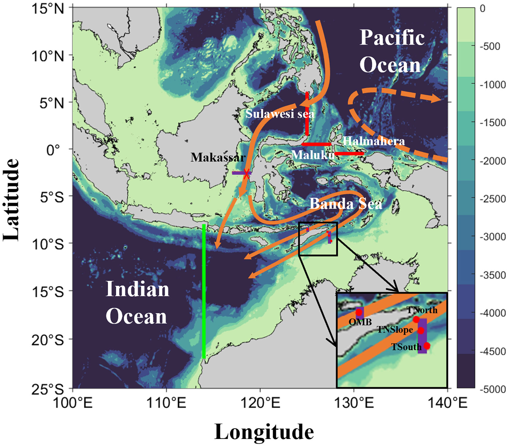
Figure 1 The topographic map of the Indonesian sea and the main flow system of the ITF. The pathways of ITF are shown by orange lines with arrows. The red $\times$ indicates the mooring station in the Makassar Strait. The four red dots that appear in the enlarged view in the small window of the lower right corner denote the mooring positions of the Ombai and Timor Straits, and from north to south are Ombai Strait (OMB), Timor North (TNorth), Timor North Slope (TNSlope), and Timor South (TSouth), the first of which is the mooring position of the Ombai Strait and the remaining three are the mooring positions of the Timor Strait. The purple lines are the interception position of the corresponding strait data validation. The dotted arrows in orange represent the Pacific Ocean flow. The red and green solid lines indicate the inflow and outflow cross-sections, respectively.

3.1 Validation of model data

Performances of the four reanalysis datasets are validated by using the mooring observation located at the Makassar Strait, namely the INSTANT and MITF programs. In accordance with the two periods of INSTANT and MITF, the comparative results are divided into two stages, which are January 2004 to late November 2006 and November 2006 to August 2017, respectively. An approximate position at the same latitude as the mooring position is selected to conducted verification when calculating the Makassar Strait flow, which is 117°E–119°E, 2.5°S (Figure 1).

The comparative results are illustrated in Figures 2A, B. In the upper layer, the mean mooring transport is -7.94 Sv (negative means southward transport). It shows a prominent interannual variability. The transport intensified from 2004 to late 2008, with an intensification of -1.53 Sv, whereas from 2009 to mid–2011, it slightly weakened by 0.32 Sv. The transport quickly weakened from mid–2013 to mid–2016, whereas the ITF quickly intensified. The relativity between the upper and lower layers was negative and insignificant (correlation coefficient of -0.30). In the lower layer, the mean transport is -3.10 Sv. The trends of mean transport during 2004–2011 and 2013–2017 were the opposite: there is an intensified (weakened) trend in the former period and a weakened (intensified) trend in the latter period in the upper (lower) layer. In addition, in terms of interdecadal variability, the correlation between the upper layer Makassar flow and PDO and NPO were significantly opposite (Figures not shown). During 2004–2011 and 2013–2017, the correlation coefficients between PDO and flow in the upper layer were 0.78 and 0.75, respectively; whereas the correlation coefficients between NPO and flow changes in the upper layer were -0.44 and -0.35, respectively. All the correlation coefficients pass the 95% significance test. However, the contributions of PDO in the ITF transport are limited in the upper layer inflow and in the decadal timescales, which will not be further considered in this study.

FIGURE 2

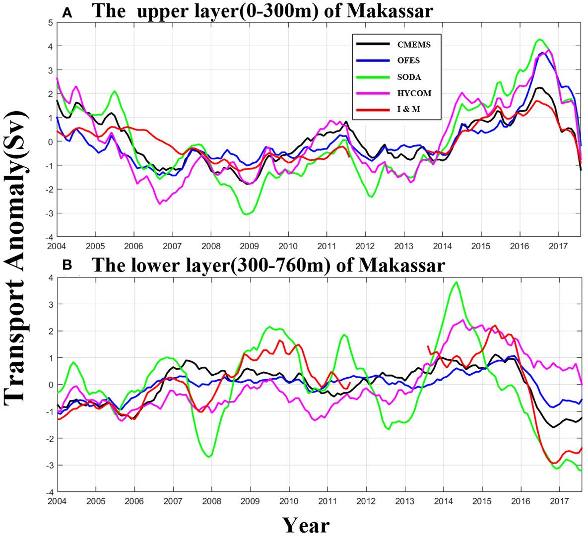
Figure 2 Transport anomaly of the four reanalysis datasets and the mooring observation at Makassar. (A) Transport in the upper layer. The red line is the mooring observation of INSTANT and MITF after a 13-month moving average. The black, blue, green, and pink lines are CMEMS, OFES, SODA, and HYCOM, respectively. Due to the discontinuity of mooring data between 2004 and 2017, the correlation coefficients of the first and second halves of the mooring after the 13-month moving average are calculated, respectively. (B) Same as (A) but for the lower layer. Negative values mean southward transport anomaly.

In the upper layer, the correlation coefficients of SODA and CMEMS in the first and second periods are R1 = 0.8 and R2 = 0.96, respectively, and the RMSE is 1.12 Sv, in comparison with the observed data. Similarly, the OFES data in this layer exhibit low correlation coefficients with the observed data in the first half and the second half, where R1 = 0.25 and R2 = 0.7, respectively, and the RMSE is 0.82 Sv. It can be found that between July 2005 and November 2006, the reanalysis data declined more than the mooring observation data, which may be explained by that single point data of Makassar mooring could not accurately reflect the whole change in the entire channel. In the lower layer, the correlation coefficients of OFES and CMEMS with the observed data in the first and second half are R1 = 0.73 and R2 = 0.98, respectively, and the RMSE is 0.89 Sv. The HYCOM data in this layer has relatively low correlation coefficients of R1 = 0.49 and R2 = 0.77, respectively, and the RMSE is 1.35 Sv, in comparison with the observed data. All the correlation coefficients pass the 95% significance test. It can be found that in the upper and lower layers, the correlation between the reanalysis and mooring observation data in the second period is better than in the first period, which may be attributed to the reanalysis datasets dependency and the limitation of mooring observations.

The mooring data of the Ombai and Timor Straits are comprehensively collected to verify the applicability of reanalysis data in the outflow area. Two sections along 125.08°E, 8.33°S–8.83°S and 127.35°E, 8.71°S–10.02°S in the Ombai and Timor Straits, respectively, are selected to conduct the calculation. The low resolution of SODA (only 0.1°) leads to a lack of lower layer data in the Ombai Strait, and hence, only the upper layer of SODA is given below.

Figures 3A, B illustrate the comparison results in the Ombai Strait. For SODA, the correlation with the observed data is low due to the low resolution in the upper layer (R = 0.31, which passes the 95% significance test; RMSE = 0.61 Sv). Apart that, the correlations of the other three reanalysis data are all high. Among them, correlation coefficient of OFES is maximum which reaches 0.90 and RMSE is 0.45 Sv. In the lower layer, HYCOM has the maximum correlation coefficient of 0.80 and lowest RMSE of 0.28 Sv, whereas OFES has a relatively low correlation coefficient of 0.69 and RMSE of 0.43 Sv. The validation results of the Timor Strait data are shown in Figures 3C, D. It is found that CMEMS has the maximum correlation coefficient of 0.71 and lowest RMSE of 0.14 Sv in the upper layer, whereas HYCOM has a relatively low correlation coefficient of 0.38 (passing the 95% significance test) and RMSE of 0.26 Sv. In the lower layer, CMEMS also exhibits a good correlation, with a correlation coefficient of 0.63 and RMSE of 0.11 Sv. However, the correlation coefficients of the other three data are low. Note that, all the correlation coefficients pass the 95% significance test, which demonstrate that all the four reanalysis datasets show consistency with the observations, which gives the confidences to use the reanalysis datasets to show the variability and mechanisms.

FIGURE 3

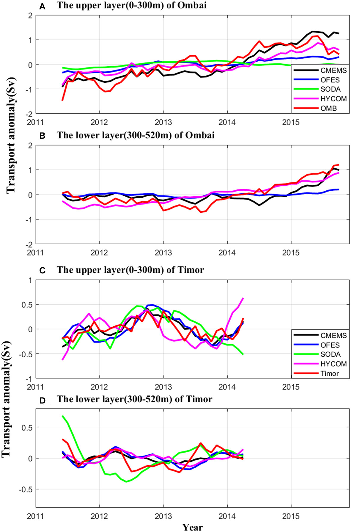
Figure 3 Transport anomaly of the four reanalysis datasets and the mooring observation in the Ombai and Timor Straits. (A) Transport in the upper layer of Ombai Strait. The red line is the mooring observation of Ombai Strait after a 13-month moving average. The black, blue, green and pink lines are CMEMS, OFES, SODA and HYCOM, respectively. (B) Same as (A) but for the lower layer of Ombai Strait. (C, D) Same as (A, B) but for Timor Strait. Negative values mean southward transport anomaly.

3.2 Spatial and temporal variability of the ITF

Good performance of the eddy-resolving reanalysis datasets reveals, the detailed spatial structures of the ITF in the inflow and outflow.

Among the three inflow cross-sections (Figures 4A–C), the Sulawesi Sea has the widest entrance, which spans 3.58°N–5.5°N, 125°E. There are two opposite flows, which are westward in the northern channel and eastward in the southern channel, respectively. As the depth deepens, the eastward flow gradually expands to the north, while the westward flow decreases in scope. The eastward flow mainly exists in the range of 125°E, 1.83°N–3.5°N (the maximum depth is 350 m south of 3.25°N, while it can be extended to 760 m north of 3.25°N), with an average speed of 0.07 m s^-1 and a maximum speed of 0.23 m s^-1 at a depth of 20m near 2.25°N. The westward flow in the 3.58°N–4.66°N region mainly exists above the 115 m layer with an average speed of -0.14 m s^-1. The large value zone of westward flow mainly exists in 4.5°N–5.33°N (the depth can be extended to 760 m) and a maximum speed is -0.59 m s^-1 at a depth of 85 m near 5°N. There is a weak eastward flow near Mindanao Island. The standard deviation of the flow gradually decreases with the increase of depth overall. There has a larger standard deviation in the westward flow, which can reach 0.13 m s^-1, mainly concentrated in the upper 90 m layer of 4.58°N–5.08°N. In the eastward flow range, the standard deviation of the flow can reach a maximum of 0.09 m s^-1, mainly concentrated in the surface layer of 1.91°N–2.83°N.

FIGURE 4

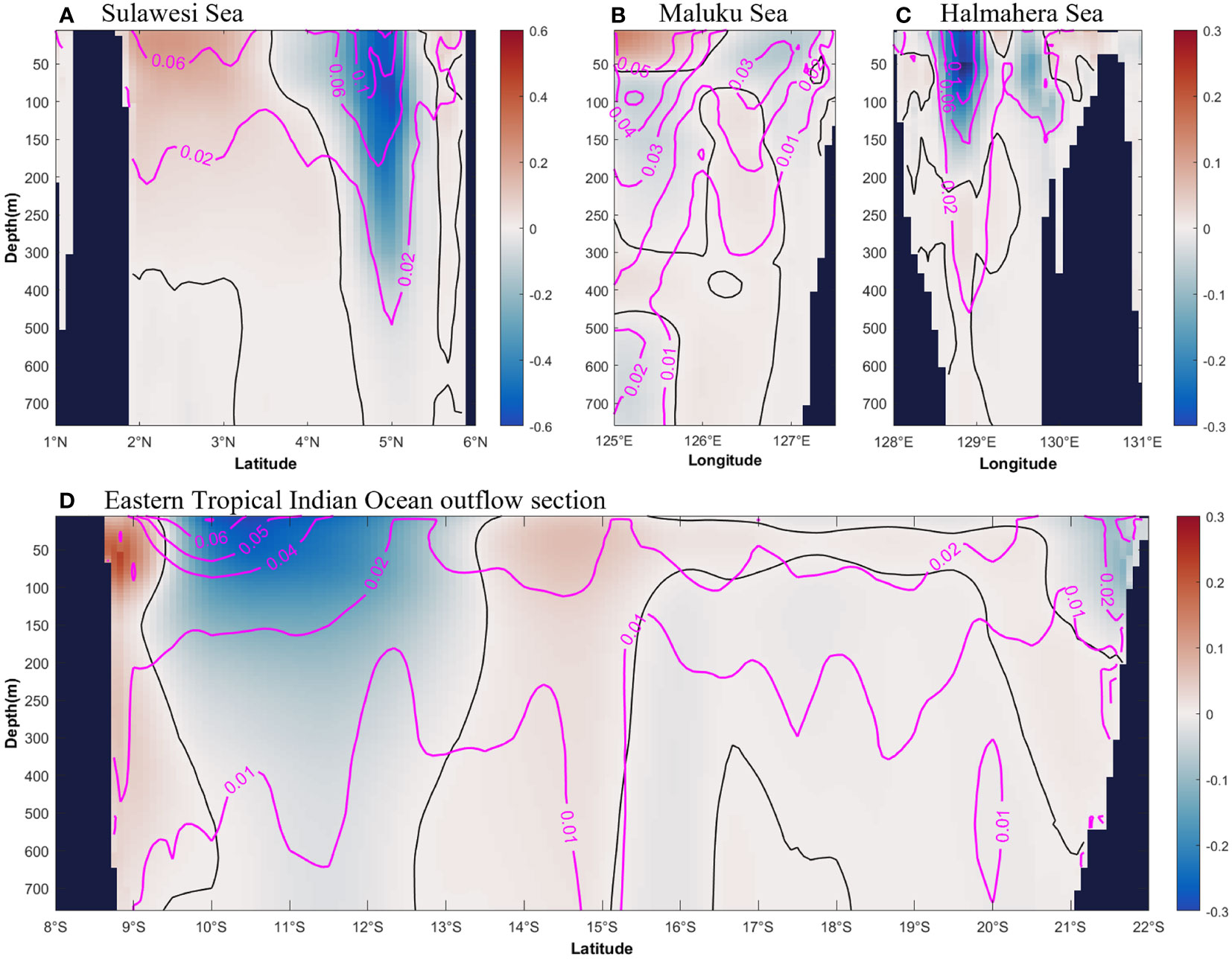
Figure 4 The four reanalysis datasets average velocity in the inflow (upper panel) and outflow (lower panel) cross-sections from 1993 to 2019. The profile color fill is the East-West (North-South) velocity of the flow perpendicular to the longitude (latitude). (A, D) are the zonal flow in the Sulawesi Sea and the eastern equatorial Indian Ocean cross-sections, respectively. (B, C) are zonal flows in the Maluku Sea and the Halmahera Sea cross-sections, respectively. The magenta contour is represented as the standard deviation of the flow velocity of each section on the interannual scale. The black contour line in the figures indicate that the velocity is 0. A negative value represents southward or westward flow.

The opposite flow structure is the same as the Maluku Sea meridional sections (Figure 4B). In the western Maluku Sea (125°E–126°E, 0.5°N): above 60 m layer, it flows northward with an average speed of 0.05 m s^-1, and the maximum is 0.16 m s^-1 at a depth of 10 m near 125°E; within a depth of 60 m–300 m, it flows southward with an average speed of -0.02 m s^-1, and the flow gradually decreases as the depth increases; within a depth of 300 m–450 m, there is a weak northerly flow; under 450 m, there is a southward flow, which corresponds well to the observational finding of the Maluku Sea intermediate western boundary current (Yuan et al., 2022). In the eastern Maluku Sea (126°E–127.5°E, 0.5°N): above 60 m layer, there is a weak southward flow with an average speed of -0.03 m s^-1 and the maximum southward flow velocity is -0.07 m s^-1; under 60 m, except for the presence of weak southward flow in depth of 350 m–720 m and range of 126°E–126.41°E, it flows northward in the western side (126°E–126.83°E, 0.5°N) and southward on the eastern side (126.83°E–127.5°E, 0.5°N). The large standard deviation of the flow velocity is mainly concentrated in the western upper layer of Maluku Sea (125°E–126°E, 0.5°N), which can reach a maximum of 0.07 m s^-1. With the increase of depth, the standard deviation gradually decreases. However, below 450 m in the western of Maluku Sea, there is still a relatively large variation zone with a standard deviation of 0.02 m s^-1.

In the Halmahera Sea section (0.5°S) (Figure 4C), the flow structures are complicated. In the range of 128.5°E–129.75°E and 129.91°E–130.08°E, there are southward flows, which can reach a depth of 200 m. The maximum velocity (-0.36 m s^-1) appears at 128.83°E and 50 m depth. The flow is northward at both sides of the Halmahera Sea section and in the lower layer. However, the northward flow is relatively weak, with a maximum of 0.08 m s^-1. The large standard deviation of flow velocity is concentrated in the large value region of southward flow, which can reach a maximum of 0.14 m s^-1 in the upper layer of 128.83°E. With the increase of depth, the standard deviation gradually decreases. At the maximum southward flow (at 128.83°E and 50 m depth), the standard deviation reaches 0.12 m s^-1.

In the exit of the eastern equatorial Indian Ocean (Figure 4D), the outflow is a significant eastward flow in the 0–110 m range of 114°E, 8.75°S–9.33°S, and the maximum velocity is 0.22 m s^-1 at a depth of 60 m at 8.83°S. The eastward flow corresponds to the upper ocean South Java Coastal Current (SJCC) (Atmadipoera et al., 2009; Sprintall et al., 2009; Liang and Xue, 2020). In the middle section of 114°E, 9.5°S–13.41°S, most of the flow is westward with a maximum of -0.28 m s^-1, which exists at a depth of 10 m at 10.5°S. The eastward flow south of 14°S is closely related with the Eastern Gyral Current (EGC) and the Northwest Shelf Inflow (NWS-inflow) (Liang and Xue, 2020). The large standard deviation values of flow velocity are concentrated in the range of westward flow, which can reach 0.06 m s^-1 in the upper layer.

The comparison results reveal a narrower and stronger inflow and a wider and weaker outflow. This opposite flow among the cross-sections implies complicated flow structures in the high-resolution reanalysis datasets. Detailed flow structures along with additional field experiments should be verified.

To understand the interannual variations of the ITF transport, the upper, lower and full depth layers of the inflow and outflow transport anomaly are illustrated in Figure 5. The results are averaged from the four reanalysis datasets. In the upper layer (Figure 5A), the linear trends of inflow and outflow are -0.08 Sv year^-1 and -0.04 Sv year^-1, respectively (negative linear trend indicates an increase in southwesterly flow). During the strong El Niño event (1997/1998), there was a significant decrease in the upper layer inflow, with a value of -3.38 ± 4.15 Sv. It applies to 2015/2016 as well, when the upper layer inflow is -4.90 ± 1.98 Sv. During positive IOD events (2004–2008), the upper layer inflow increased significantly, from -5.31 ± 2.76 Sv in 2004 to -14.31 ± 4.14 Sv in 2008. However, the upper layer outflow intensified only during 2005–2006, which was significantly weaker than the inflow. In the upper layer outflow, the interannual variation is similar to those of the inflow, the average correlation coefficient between the upper layer inflow and outflow of the four models is 0.63, which passes the 99% significance test. The average flow is more intensified than the upper layer inflow, and the difference is 3.23 Sv. In the upper layer, it can be found that the inflow is smaller than the outflow, which is mainly due to the reason that the South China Sea (SCS) branch of the ITF is not taken into account. Note that, the depth of the Karimata Strait that connects the SCS and Indonesian Sea is less than 50 m, so its inflow mainly contributes to the upper layer.

FIGURE 5

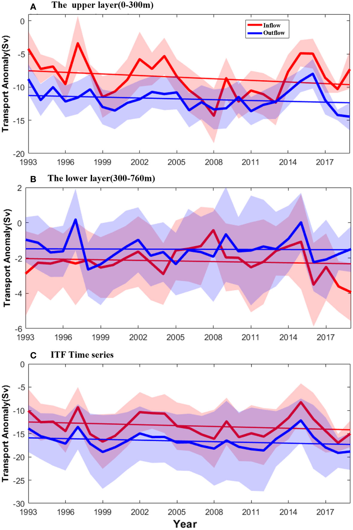
Figure 5 Interannual variability of the ITF transport in different layers. (A) The four reanalysis datasets average the upper layer inflow and outflow from 1993 to 2019. The red and blue lines represent inflow and outflow, respectively. The shaded areas indicate the standard deviation. (B, C) Same as (A) but for the lower layer and full depth (0 to the maximum modeling depth), respectively. Negative values mean southward or westward transport anomalies (enhanced ITF).

Unlike the upper layer, the lower layer flow shows no significant trend in the interannual scale (Figure 5B). For the lower layer inflow, the flow decreased in 2015 and increased in 2016, but with a much smaller amplitude than that of the upper layer. The lower layer outflow in the same period was also similar. In 1997, the lower layer outflow showed a similar change as the upper layer. In the lower layer, it can be found that the outflow is greater than the inflow, which is closely related to the large inflow of HYCOM.

The total ITF transport is obtained in Figure 5C. The results show that the average ITF transport is -13.33 Sv and -16.62 Sv of the inflow and outflow, with linear strengthening trends of -0.06 Sv year^-1 and -0.05 Sv year^-1, respectively. On average, the outflow value is larger than the inflow. The outflow volume transport estimated in this study is -16.62 Sv, which is close to that by SODA (-16.9 Sv) and the multi-model ensemble means of phase 5 of the Coupled Model Intercomparison Project (CMIP5) (-15.3 Sv) (Santoso et al., 2022). In the Makassar Strait, the mooring average flow of the upper (-9.10 Sv) and lower layers (-3.40 Sv) from 2004 to 2017 (Gordon et al., 2019) are consistent with the reanalysis datasets, which is -9.36 Sv in the upper layer and -1.88 Sv in the lower layer. The difference in the outflow and inflow (3.29 Sv) is larger than in the Makassar Strait (1.26 Sv). Two possible reasons contribute to the mismatch between the inflow and the outflow. First, the SCS branch of the ITF and the inflow along the northern Australia coast are not taken into account in the inflow and outflow calculation, which results in small and large estimates of the inflow and outflow, respectively. Results of the previous particle tracking experiments present the interannual average of the ITF branch in the South China Sea to be approximately 1.6–1.98 Sv (He et al., 2015; Xu et al., 2021). Most of the reanalysis data show that the inflow after adding Karimata Strait flow is comparable to the outflow. And for the high spatial resolution data (CMEMS, HYCOM), the inflow adding Karimata Strait flow is comparable to the outflow after subtracting the inflow along the northern Australia coast. Second, different reanalysis data show large dispersions in the ITF estimation. The full-depth ITF obtained by four kinds of reanalysis data (CMEMS, SODA, OFES, HYCOM) at the inflow position is -14.22 Sv, -15.01 Sv, -6.44 Sv, and -16.94 Sv, respectively. At the outflow position, they are -17.28 Sv, -15.20 Sv, -8.95 Sv, and -24.29 Sv, respectively. The differences are 3.06 Sv, 0.19 Sv, 2.51 Sv, and 7.35 Sv, respectively. The largest deviation between the outflow and the inflow is derived from the HYCOM dataset. In addition, the selection of the outflow section also affects the amount of transport. Overall, it is reasonable to use reanalysis data in this study to reflect the interannual changes of ITF.

4 Contribution of ENSO and IOD to the ITF transport

4.1 Relationships between climate modes and ITF transport

Figure 6 illustrates the variabilities of ITF transport in different layers that further explain the correlations between the climate modes and the detailed flow structure. For the upper layer inflow, the correlation coefficients between flow data and Niño 3.4, DMI, and CP indices are 0.73, -0.28, and 0.56, respectively. Among the above results, Niño 3.4 and CP pass the 99% significance test, whereas DMI does not pass the 95% significance test. In the lower layer inflow, the correlation coefficient between flow anomaly and Niño 3.4, DMI and CP indices are 0.23, 0.01 and 0.12, respectively, none of them pass the 95% significance test. This concludes that the influence of the climate index in the upper layer is greater than that in the lower layer.

FIGURE 6

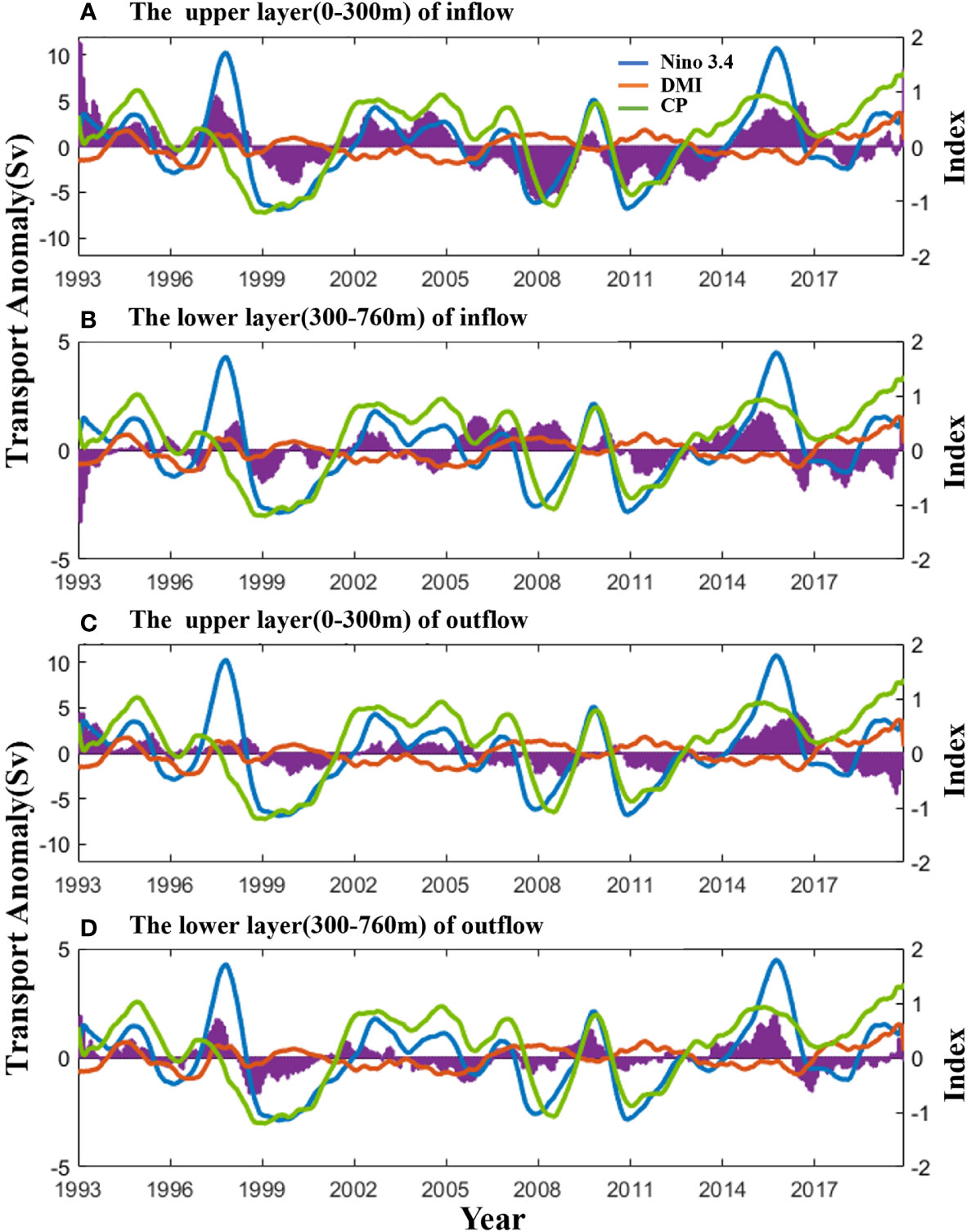
Figure 6 Interannual variations of the ITF transport anomaly and the climate indices. (A) The four datasets average the upper layer inflow transport anomaly (purple shadow), superimposed with the three indices (Niño 3.4-blue, DMI-orange, CP-green) after a 13‐month running mean. The DMI is the $DM{I}_{new}$ after removing the linear influence of Niño 3.4. (B) Same as (A) but for the lower layer inflow. (C, D) The upper layer and the lower layer outflow transport.

In the upper layer outflow, the correlation coefficients between flow data and Niño 3.4, DMI, and CP indices are 0.52, -0.55, and 0.32, respectively. Among the above results, Niño 3.4 and DMI pass the 99% significance test, whereas CP does not pass the 90% significance test. In the lower layer outflow, the correlation coefficients of flow anomaly with Niño 3.4 and CP indices are 0.65 and 0.41, respectively, and they pass the 99% significance test, whereas the correlation coefficient with the DMI shows a low correlation (0.12). The correlation between Niño 3.4 and CP indices, and the lower layer is greater than the correlation of the upper layer inflow. Whereas, the correlation between the DMI index and the lower layer with that of the upper layer inflow is the opposite.

Niño 3.4 and DMI have opposite correlations for ITF in comparison with the upper layer inflow and outflow. The linear correlation coefficients between Niño 3.4 and ITF anomalies remained high at 0.73 and 0.52 for the inflow and outflow, respectively. However, the DMI is -0.28 and -0.55 in the inflow and outflow, respectively, and the correlation changes are relatively large. The conclusion is consistent with Li et al. (2020). In the upper layer, the CP index maintains a positive correlation with both inflow and outflow, which is similar to the impact of the Niño 3.4 index. The difference with Li et al. (2020) is that the Niño 3.4 and CP indices have a strong positive correlation with the lower layer outflow, which may be related to the period selected.

4.2 Relative importance of climate modes in the ITF variability

To quantitively expose the climate drivers of ITF transport, the RF method is adopted in this subsection. Before that, the dominant periods of the ITF transport should be clarified. The average multi-models flow data in different levels (Figure 7) help to obtain the power spectra of the upper layer and the lower layer inflow and outflow during 1993–2019. Power spectral analysis reveals that the upper layer and the lower layer inflow exhibit peak periods of 4–9 and 5–7 years, respectively. The upper layer and the lower layer outflow exhibit peak periods of 5–7 and 2–6 years, respectively. Overall, the results characterize a common peak period flow of 5–7 years at four different locations. Comparatively, Niño 3.4, as well as DMI and CP indices have peak periods of 2–7, 2–4, and within 10 years (Sullivan et al., 2016; Santoso et al., 2022), respectively.

FIGURE 7

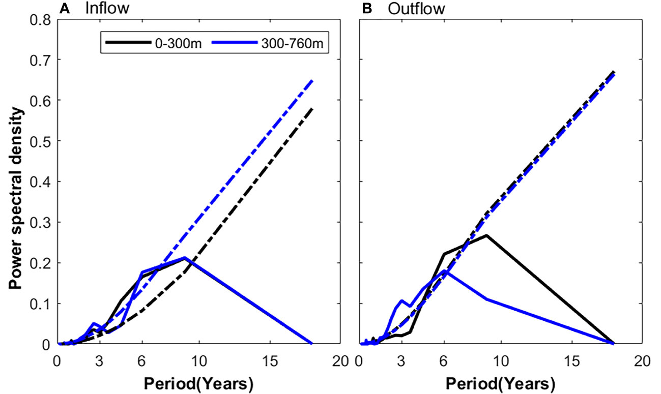
Figure 7 The power spectrum of inflow and outflow at different levels. The flow data is the multi-models average monthly data after a 13-month sliding average from 1993 to 2019. (A) The black and blue solid lines represent the result of the upper layer (0–300 m) and the lower layer (300–760m) inflow, respectively. The black and blue dotted lines represent their 95% confidence level. (B) same as (A) but for outflow.

The calculation of the power spectrum of the four levels of flow data and climate indices concludes that the main change cycle is concentrated in 5–7 years; hence, it is taken as the cycle for RF model training. In addition, to make full use of the data and the experimental results more reliable, the data is recycled (consider the 6-year cycle as an example: 1993–1998, 1994–1999…). Niño and IOD events often occur simultaneously during RF model training. Therefore, the $DM{I}_{new}$, which removes the influence of the linear trend of Niño 3.4, is adopted and the corresponding RF models by using four model data training are obtained. The relative importance of the RF training results in the period of 5, 6, and 7 years, respectively, are considered. Significant differences are not revealed in the results (figures not given). Therefore, the 6–year period is considered to reveal the relative importance of different climate indices at different levels, beginning with different starting years (Figure 8). Due to the OFES data is up to 2017, the results for the starting year 2013–2014 are obtained from CMEMS, HYCOM, and SODA data. In this study, the dominant index is defined as the importance higher than 33% and which exceeds the other two indices without overlapping.

FIGURE 8

Figure 8 The importance of climate indices on the ITF transport. (A) The importance of climate indices (Niño3.4 blue, DMI red, CP green) in the upper layer inflow with a 6–year cycle. The triangles represent the major ENSO and IOD events that occur in the corresponding starting year, where the upper and lower edges represent ENSO and IOD events, respectively, and the solid and hollow indicate positive and negative anomalies, respectively. (B–D) same as (A) but for the lower layer inflow, the upper layer outflow, and the lower layer outflow, respectively. The shaded areas indicate the standard deviation. The dominant driver defined in this study is the one with the largest proportion and does not overlap with the other two indices.

The RF results show that in the upper layer inflow, starting from 1993–1995 (end of 2008 and 2000), the importance of the Niño 3.4 was significantly higher than that of the other two indices which was greater than 40%. In the 1996–2001 period (end of 2001 and 2006), Niño 3.4 showed more important but insignificant results (shadow regions cover each other) under the average training results of multi-model data. In the starting year of 2002–2003 (end of 2007 and 2008), the DMI became the important index (without overlap of the other two indices). In the periods of 2004–2012 (end of 2009 and 2017), the relative importance of the three indices were comparative and the overlapping shadow covered each other. In the periods of 2013–2014 (end of 2018 and 2019), the importance of the DMI increased, whereas the importance of the Niño 3.4 decreased.

Different from the upper layer, in the lower layer inflow, in the starting year of 1993 (end of 1998), the DMI was relatively important. However, in the starting year of 1994 (end of 1999), the importance of DMI decreased and CP was relatively important. In the starting years of 1995–1999 (end of 2000 and 2004), the shadows of the three indices overlapped each other. On average, the CP was relatively important but insignificant. In the initial years of 2000–2007 (end of 2005 and 2012), the importance of DMI gradually increased, and during 2002–2003 (end of 2007 and 2008), DMI had significant importance. In the later period, starting from 2008–2014 (end of 2013 and 2019), the error bars of the three indices overlapped, and again, there was no dominant index.

In the upper layer outflow, the Niño 3.4 was always at a high level during the 1993–1999 period (end of 1998 and 2004), which implies the dominance of Niño 3.4. During 2000–2001 (end of 2005 and 2006), the influence of the DMI on the upper layer outflow increased, but the importance of the Niño 3.4 decreased. In the starting years of 2002–2004 (end of 2007 and 2009), the DMI became the dominant factor, with an average relative importance of more than 50% between 2002 and 2007. In the initial years of 2005–2007 (end of 2010 and 2012), the average relative importance of the CP increased, but the shadow region coincided with the shadow region of the DMI. In the starting years 2008–2012 (end of 2013 and 2017), the importance of all three indices was relatively close. This indicates the complexity of the influencing factors of ITF during this period, and a significant index was not identified. In the following starting years 2013–2014 (end of 2018 and 2019), the DMI became the dominant factor again, with an average relative importance of more than 40%.

In the lower layer outflow, starting from 1993–1995 (end of 1998 and 2000), the error bars of the three indices coincided, and the significant index was not dominated. In the starting years of 1996–1998 (end of 2001 and 2003) and 2013–2014 (end of 2018 and 2019), the CP was the important index, with an average proportion of 40%. In the starting years of 1999–2000 (end of 2004 and 2005) and 2009–2012 (end of 2014 and 2017), there was no dominating index. In the initial years of 2001–2005 (end of 2006 and 2010), the DMI was the important influence index, with an average proportion of 50%. In the starting years of 2006–2008 (end of 2011 and 2013), the Niño 3.4 was the dominant influence index, with an average proportion of 50% in 2007.

Figure 9 illustrates the relative importance of the different climatic factor indices and their partial dependence in different periods. In the partial dependence plots, the steeper the curve change, the greater the influence of the corresponding index. The results reveal that the curve of Niño 3.4 to be the steepest and the influence on the upper layer inflow to be the greatest during 1993–1998. In 2002–2007, the DMI curve was the steepest and became the dominant index. Similarly, in 2008–2013, the CP and Niño 3.4 were relatively important. During 2014–2019, the importance of DMI increased. The results are consistent with those in Figure 8. The partial dependences of the climate indices on the lower layer inflow, as well as the upper layer and lower layer outflows are similar to the upper layer inflow (figures not given).

FIGURE 9

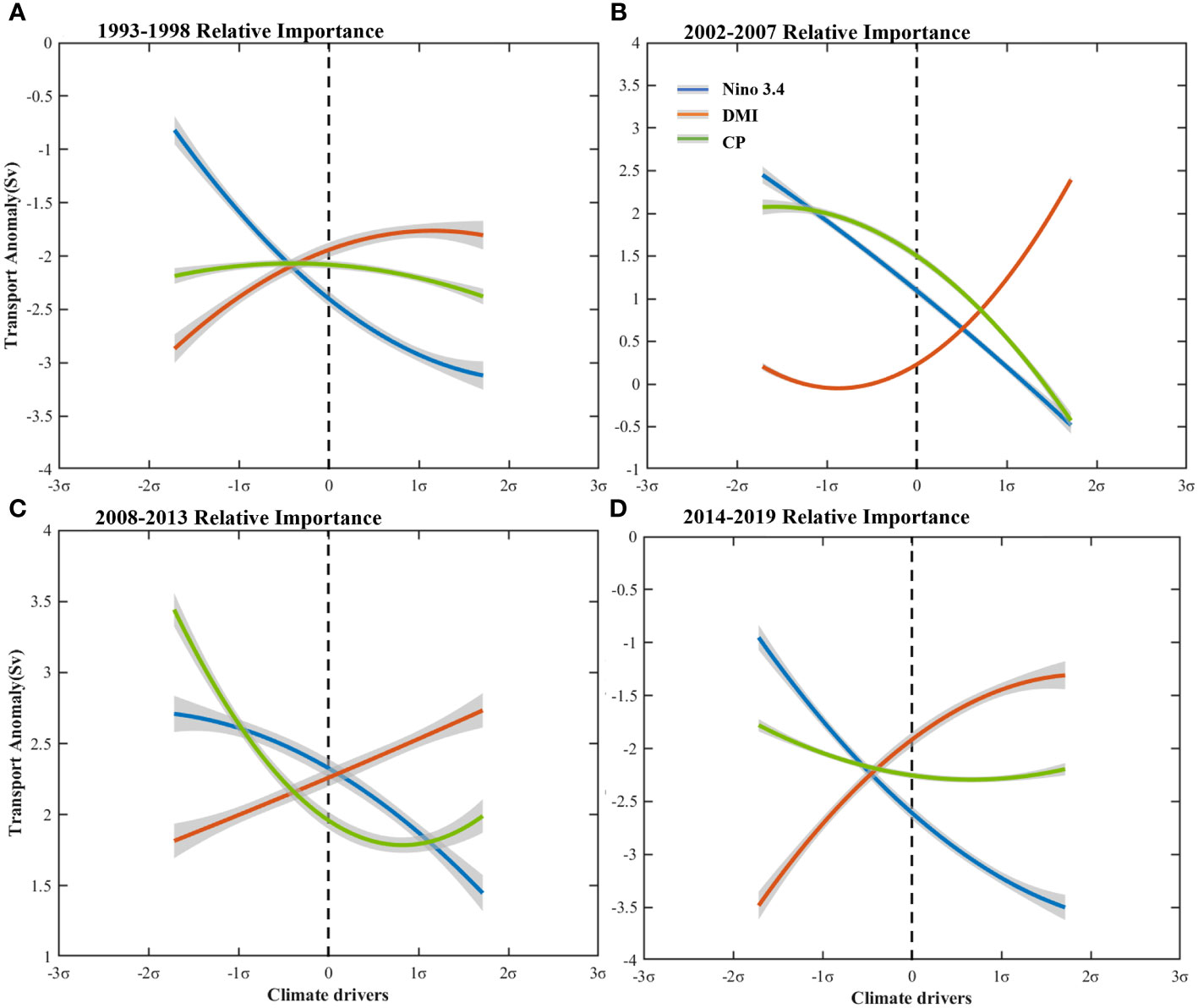
Figure 9 The partial dependence of the upper layer inflow in different sub-period from the RF model on each climatic factor index. (A) 1993–1998, (B) 2002–2007, (C) 2008–2013 and (D) 2014–2019. The blue, orange, and green lines are Niño 3.4, DMI and CP indices, respectively. The trend of the curve describes the correlation between the corresponding factor and the predictor. The shaded part represents a 95% confidence interval.

5 Discussion

The RF model shows the domination of different climate modes in different periods. To explore the underlying mechanisms, four periods of 1993–2000, 2002–2008, 2009–2012, and 2013–2019 are composited, which corresponds to the dominant factors of Niño 3.4, DMI, no significant dominant index, and DMI, respectively. Among them, the dominant DMI from 2013 to 2019 mainly exists in the upper layer outflow. Previous studies reveal that the sea surface height anomaly (SSHA) between two oceans (NWP and SEI) is regarded as a good indicator of ITF transport (Wyrtki, 1987; Shilimkar et al., 2022). This viewpoint is adopted to demonstrate the underlying mechanism.

Figure 10 presents the average of SSHA for different periods, with the spatial location of NWP and SEI marked. During the ENSO domination period (1993–2000), the mean SSH in the NWP and SEI are -0.68 cm and -0.18 cm, respectively, and the SSH difference is -0.50 cm. During the first IOD domination period (2002–2008), the NWP and SEI are 0.49 cm and -0.50 cm, respectively, and the SSH difference is 0.99 cm. During the period with no dominant climate indices (2009–2012), the NWP and SEI are 5.58 cm and 1.24 cm, respectively, and the SSH difference is 4.34 cm. During the second IOD domination period (2013–2019), the NWP and SEI are -3.59 cm and -0.37 cm, respectively, and the SSH difference is -3.22 cm. The SSH field variation in the two regions is related to the ENSO and IOD events, especially the El Niño and negative IOD events, respectively. The SSH differences between the different periods are consistent with the mechanism, that during El Niño (negative IOD) events, it reduces the Pac-Indian Ocean pressure gradient and makes a weak ITF. On the contrary, La Niña and positive IOD events help to enhance the ITF.

FIGURE 10

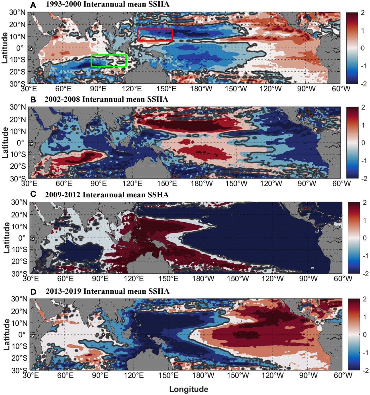
Figure 10 SSHA in different periods. (A) 1993–2000, (B) 2002–2008, (C) 2009–2012, (D) 2013–2019. The ranges in the red and green boxes in (A) are NWP (6°N–16°N, 125°E–155°E) and SEI (6°S–16°S, 85°E–115°E), respectively. The solid gray line is the contour line with SSHA of zero.

To further explore the mechanisms, the ENSO and IOD events in the years 1993–2019 are summarized in Table 1. During 1993–2000 when ENSO dominates, a strong El Niño event occurred in 1997/1998 accompanied by a positive IOD event (Figure 8A). This strong El Niño event led to reduced precipitation in the western Pacific and Indonesia, which directly led to a lower SSH at the ITF inflow position (Chandra et al., 1998; Gordon et al., 1999). Moreover, the occurrence of the positive IOD event reduced the SSH at the ITF outflow location (Cai et al., 2011). Thus, both the upper layer inflow and outflow of the ITF showed a strong reduction of 4.21 Sv and 1.21 Sv, respectively (Figure 5A). After experiencing a significantly weakened ITF in 1997/1998, the ITF returned to its previous level in late 1998 under the combined effect of La Niña and negative IOD events. Overall, it is inferred that the occurrence of the El Niño event in 1997/1998 played a dominant role in the 1993–2000 period.

TABLE 1

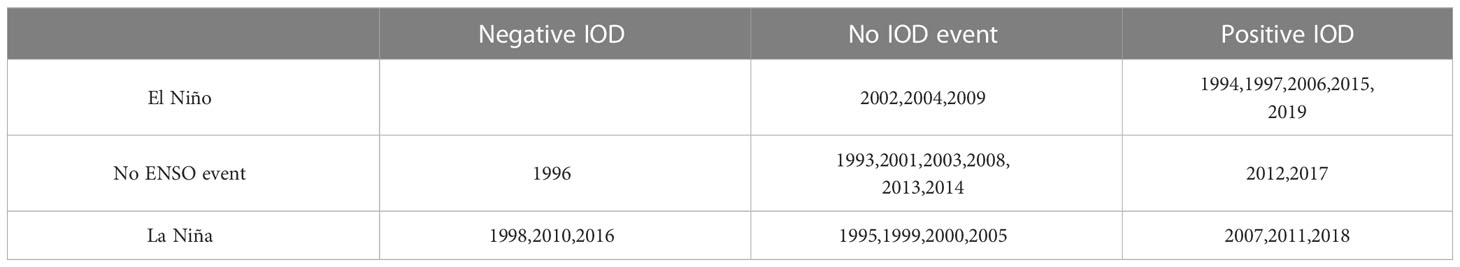
Table 1 Classification of years when El Niño or La Niña is contacted with positive IOD or negative IOD events from 1993 to 2019.

During 2002–2008 when IOD dominates, two successive positive IOD events occurred in 2006 and 2007, corresponding to the El Niño and La Niña events, respectively (Figure 8A). The positive IOD events are strongly associated with the Indian Ocean surface temperature anomalies (unusually cold in the east and warm in the west), further leading to a low SSH in the eastern Indian Ocean (Behera et al., 2008). During 2004–2008, both the upper layer inflow and outflow were enhanced 2.08–2.79 Sv (Figure 5A). During 2002–2008, the SSH differences between NWP and SEI was 0.99 cm, which partly explains the dominant effect of the IOD events. This concluded that the IOD events dominated the variability of the ITF transport during 2002–2008.

During 2009–2012 when no climate indices dominate, the successive La Niña events in 2010 and 2011 and the successive positive IOD events in 2011 and 2012 (Figure 8A), which partly explained that there were no single climate mode playing the dominant role during this period.

During 2013–2019 when IOD dominates in the upper layer outflow, it also corresponded to the sharp decrease in the upper layer outflow during 2015–2016 (Figure 5A) and the SSH difference between NWP and SEI was -3.22cm. During this period, relatively strong negative IOD event occurred in 2015/2016 (Figure 8A). Pujiana et al. (2019) also revealed that the sharp decrease in the upper layer inflow and outflow in 2015/2016 was attributed to the strong negative IOD events. In addition, successive positive IOD events occurred from 2017 to 2019, which further illustrated the dominant effect of IOD events.

6 Conclusions

In this study, the spatial and temporal variabilities of ITF are obtained in the four high-resolution reanalysis datasets (three are eddy-resolving and one is eddy-permitting models). The ITF is further divided into the upper layer and the lower layer flow, respectively. The results of spatial structure analysis reveal that among the three inflow passages, the Sulawesi Sea is the main inflow area in terms of inflow and the maximum westward flow velocity reaches -0.59 m s^-1. In terms of outflow, the range of 9.5°S–13.41°S and 114°E in the eastern equatorial Indian Ocean cross-section is the main outflow area, and the maximum westward flow velocity reaches -0.28 m s^-1. The temporal analysis results reveal that the southwest flow of the upper layer inflow and outflow have interannual enhanced trends, which are -0.08 Sv year^-1 and -0.04 Sv year^-1, respectively, whereas the lower layer inflow and outflow do not have obvious linear trends on the interannual scale. The interannual average of ITF full-depth flow is -14.97 Sv, whereas the linear enhanced trend is -0.06 Sv year^-1.

During 1993–2019, the linear correlation coefficients of Niño 3.4 index and flow change are greater than those of DMI index and CP index at the upper layer and the lower layer inflow and the lower layer outflow, while the upper layer outflow shows a strong correlation with DMI index. To quantify the relative importance of the three climate factors to ITF changes over time, RF models are conducted at different levels. Through the analysis of the model results, the dominant climate factors of the upper layer inflow and outflow are clear in the three periods of 1993–2000, 2002–2008, and 2009–2012, which are dominated by Niño 3.4 (relative importance reaching 40%), DMI (relative importance exceeding 50%), and no significant dominant index. During 1993–2000, the El Niño event in 1997/1998 and the -0.5 cm SSH difference between NWP and SEI dominated the Niño 3.4 index. During 2002–2008, the dominant DMI was reinforced by successive positive IOD events in 2006–2007 and the 0.99 cm SSH difference between NWP and SEI. In the upper layer outflow, the dominant climate factor is clear in 2013-2019 period, which are dominated by DMI (relative importance reaching 40%). In the upper layer outflow, during 2013–2019, relatively strong negative IOD event in 2015/2016, the -3.22cm SSH difference between NWP and SEI, and successive positive IOD events occurred from 2017 to 2019 dominated the DMI index.

The climate drivers can markedly regulate the ITF transport. However, due to the complexity of the climate modes and the interaction between them, it is difficult to clarify the relative importance of each period (Wang et al., 2022). This study provides a new insight to quantify the response of ITF transport to climate drivers. However, the effect of climate factors on ITF in specific years could not be analyzed in detail. The influence of these factors on ITF changes in a specific climatic event can be studied with this method using identified significantly important climate factors.

Data availability statement

The original contributions presented in the study are included in the article/supplementary material. Further inquiries can be directed to the corresponding author.

Author contributions

YZ convinced the work, and AL performed the data analysis and wrote the original manuscript. YZ and AL improved the manuscript. All authors discussed and contributed to the writing.

Funding

This work was financially supported by Laoshan Laboratory (No. LSKJ202202704).

Acknowledgments

We sincerely thank Integrated Marine Observing System (IMOS) for providing the mooring data in the Ombai and Timor Straits.

Conflict of interest

The authors declare that the research was conducted in the absence of any commercial or financial relationships that could be construed as a potential conflict of interest.

Publisher’s note

All claims expressed in this article are solely those of the authors and do not necessarily represent those of their affiliated organizations, or those of the publisher, the editors and the reviewers. Any product that may be evaluated in this article, or claim that may be made by its manufacturer, is not guaranteed or endorsed by the publisher.

References

Anderson W. K., Thomas J. L., Van Leer B. (1986). Comparison of finite volume flux vector splittings for the Euler equations. AIAA J. 24 (9), 1453–1460. doi: 10.2514/3.9465

CrossRef Full Text | Google Scholar

Atmadipoera A., Molcard R., Madec G., Wijffels S., Sprintall J., Koch-Larrouy A., et al. (2009). Characteristics and variability of the Indonesian throughflow water at the outflow straits. Deep Sea Res. Part I: Oceanographic Res. Papers 56 (11), 1942–1954. doi: 10.1016/j.dsr.2009.06.004

CrossRef Full Text | Google Scholar

Behera S. K., Luo J. J., Yamagata T. (2008). Unusual IOD event of 2007. Geophysical Res. Lett. 35 (14). doi: 10.1029/2008GL034122

CrossRef Full Text | Google Scholar

Cai W., Sullivan A., Cowan T. (2011). Interactions of ENSO, the IOD, and the SAM in CMIP3 models. J. Clim. 24 (6), 1688–1704. doi: 10.1175/2010JCLI3744.1

CrossRef Full Text | Google Scholar

Chandra S., Ziemke J., Min W., Read W. (1998). Effects of 1997–1998 El nino on tropospheric ozone and water vapor. Geophys. Res. Lett. 25 (20), 3867–3870. doi: 10.1029/98GL02695

CrossRef Full Text | Google Scholar

Chu P. C. (1995). P-vector method for determining absolute velocity from hydrographic data. Marine Tech. Soc. J. 29 (2), 3–14.

Google Scholar

Du Y., Qu T. (2010). Three inflow pathways of the Indonesian throughflow as seen from the simple ocean data assimilation. Dyn. Atmos. Oceans 50 (2), 233–256. doi: 10.1016/j.dynatmoce.2010.04.001

CrossRef Full Text | Google Scholar

Feng X., Liu H., Wang F., Yu Y., Yuan D. (2013). Indonesian Throughflow in an eddy-resolving ocean model. Chin. Sci. Bull. 58, 4504–4514. doi: 10.1007/s11434-013-5988-7

CrossRef Full Text | Google Scholar

Feng M., Meyers G., Wijffels S. (2001). Interannual upper ocean variability in the tropical Indian ocean. Geophys. Res. Lett. 28 (21), 4151–4154. doi: 10.1029/2001GL013475

CrossRef Full Text | Google Scholar

Feng P., Wang B., Macadam I., Taschetto A. S., Abram N. J., Luo J.-J., et al. (2022). Increasing dominance of Indian ocean variability impacts Australian wheat yields. Nat. Food 3 (10), 862–870. doi: 10.1038/s43016-022-00613-9

PubMed Abstract | CrossRef Full Text | Google Scholar

Godfrey J. (1996). The effect of the Indonesian throughflow on ocean circulation and heat exchange with the atmosphere: a review. J. Geophys. Res. Oceans. 101 (C5), 12217–12237. doi: 10.1029/95JC03860

CrossRef Full Text | Google Scholar

Gordon A. L. (1986). Interocean exchange of thermocline water. J. Geophys. Res. Oceans. 91 (C4), 5037–5046. doi: 10.1029/JC091iC04p05037

CrossRef Full Text | Google Scholar

Gordon A. L. (2005). Oceanography of the Indonesian seas and their throughflow. Oceanography 18 (4), 14–27. doi: 10.5670/oceanog.2005.01

CrossRef Full Text | Google Scholar

Gordon A. L., Napitu A., Huber B. A., Gruenburg L. K., Pujiana K., Agustiadi T., et al. (2019). Makassar strait throughflow seasonal and interannual variability: an overview. J. Geophys. Res. Oceans 124 (6), 3724–3736. doi: 10.1029/2018JC014502

CrossRef Full Text | Google Scholar

Gordon A. L., Sprintall J., Van Aken H. M., Susanto D., Wijffels S., Molcard R., et al. (2010). The Indonesian throughflow during 2004–2006 as observed by the INSTANT program. Dyn. Atmos. Oceans 50 (2), 115–128. doi: 10.1016/j.dynatmoce.2009.12.002

CrossRef Full Text | Google Scholar

Gordon A. L., Susanto R. D., Ffield A. (1999). Throughflow within makassar strait. Geophys. Res. Lett. 26 (21), 3325–3328. doi: 10.1029/1999GL002340

CrossRef Full Text | Google Scholar

Gordon A., Susanto R., Ffield A., Huber B., Pranowo W., Wirasantosa S. (2008). Makassar strait throughflow 2004 to 2006. Geophys. Res. Lett. 35 (24). doi: 10.1029/2008GL036372

PubMed Abstract | CrossRef Full Text | Google Scholar

He Z., Feng M., Wang D., Slawinski D. (2015). Contribution of the karimata strait transport to the Indonesian throughflow as seen from a data assimilation model. Cont. Shelf Res. 92, 16–22. doi: 10.1016/j.csr.2014.10.007

CrossRef Full Text | Google Scholar

Heung B., Bulmer C. E., Schmidt M. G. (2014). Predictive soil parent material mapping at a regional-scale: a random forest approach. Geoderma 214, 141–154. doi: 10.1016/j.geoderma.2013.09.016

CrossRef Full Text | Google Scholar

Hirst A. C., Godfrey J. (1993). The role of Indonesian throughflow in a global ocean GCM. J. Phys. Oceanogr. 23 (6), 1057–1086. doi: 10.1175/15200485(1993)023<1057:TROITI>2.0.CO;2

CrossRef Full Text | Google Scholar

Hu S., Sprintall J. (2016). Interannual variability of the Indonesian throughflow: the salinity effect. J. Geophys. Res. Oceans 121 (4), 2596–2615. doi: 10.1002/2015JC011495

CrossRef Full Text | Google Scholar

Hu S., Zhang Y., Feng M., Du Y., Sprintall J., Wang F., et al. (2019). Interannual to decadal variability of upper-ocean salinity in the southern Indian ocean and the role of the Indonesian throughflow. J. Clim. 32 (19), 6403–6421. doi: 10.1175/JCLI-D-19-0056.1

CrossRef Full Text | Google Scholar

IMOS. (2022). IMOS - moorings - hourly time-series product (ITFOMB, ITFTIN, ITFTSL, and ITFTIS). Available at: https://imos.org.au/data/.

Google Scholar

Lee T., Fournier S., Gordon A. L., Sprintall J. (2019). Maritime continent water cycle regulates low-latitude chokepoint of global ocean circulation. Nat. Commun. 10 (1), 2103. doi: 10.1038/s41467-019-10109-z

PubMed Abstract | CrossRef Full Text | Google Scholar

Li M., Gordon A. L., Gruenburg L. K., Wei J., Yang S. (2020). Interannual to decadal response of the Indonesian throughflow vertical profile to indo-pacific forcing. geophysical res. Letters 47 (11), e2020GL087679. doi: 10.1029/2020GL087679

CrossRef Full Text | Google Scholar

Liang L., Xue H. (2020). The reversal indian ocean waters. Geophysical Res. Letters. 47 (14), e2020GL088269. doi: 10.1029/2020GL088269

CrossRef Full Text | Google Scholar

Liu Q. Y., Feng M., Wang D., Wijffels S. (2015). Interannual variability of the I ndonesian T hroughflow transport: a revisit based on 30 year expendable bathythermograph data. J. Geophys. Res. Oceans 120 (12), 8270–8282. doi: 10.1002/2015JC011351

CrossRef Full Text | Google Scholar

Masumoto Y., Sasaki H., Kagimoto T., Komori N., Ishida A., Sasai Y., et al. (2004). A fifty-year eddy-resolving simulation of the world ocean: preliminary outcomes of OFES (OGCM for the earth simulator). J. Earth Simu. 1, 35–56.

Google Scholar

Meyers G. (1996). Variation of Indonesian throughflow and the El niño-southern oscillation. J. Geophys. Res. Oceans. 101 (C5), 12255–12263. doi: 10.1029/95JC03729

CrossRef Full Text | Google Scholar

Murtugudde R., Busalacchi A. J., Beauchamp J. (1998). Seasonal-to-interannual effects of the Indonesian throughflow on the tropical indo-pacific basin. J. Geophys. Res. Oceans. 103 (C10), 21425–21441. doi: 10.1029/98JC02063

CrossRef Full Text | Google Scholar

Pang C., Nikurashin M., Pena-Molino B., Sloyan B. M. (2022). Remote energy sources for mixing in the Indonesian seas. Nat. Commun. 13 (1), 6535. doi: 10.1038/s41467-022-34046-6

PubMed Abstract | CrossRef Full Text | Google Scholar

Pujiana K., McPhaden M. J., Gordon A. L., Napitu A. M. (2019). Unprecedented response of Indonesian throughflow to anomalous indo-pacific climatic forcing in 2016. J. Geophys. Res. Oceans 124 (6), 3737–3754. doi: 10.1029/2018JC014574

CrossRef Full Text | Google Scholar

Saji N., Goswami B. N., Vinayachandran P., Yamagata T. (1999). A dipole mode in the tropical Indian ocean. Nature 401 (6751), 360–363. doi: 10.1038/43854

PubMed Abstract | CrossRef Full Text | Google Scholar

Saji N., Yamagata T. (2003). Possible impacts of Indian ocean dipole mode events on global climate. Clim. Res. 25 (2), 151–169. doi: 10.3354/cr025151

CrossRef Full Text | Google Scholar

Santoso A., England M. H., Kajtar J. B., Cai W. (2022). Indonesian Throughflow variability and linkage to ENSO and IOD in an ensemble of CMIP5 models. J. Clim. 35 (10), 3161–3178. doi: 10.1175/jcli-d-21-0485.1

CrossRef Full Text | Google Scholar

Shilimkar V., Abe H., Roxy M. K., Tanimoto Y. (2022). Projected future changes in the contribution of indo-pacific sea surface height variability to the Indonesian throughflow. J. Oceanogr. 78 (5), 337–352. doi: 10.1007/s10872-022-00641-w

CrossRef Full Text | Google Scholar

Sprintall J., Gordon A. L., Koch-Larrouy A., Lee T., Potemra J. T., Pujiana K., et al. (2014). The Indonesian seas and their role in the coupled ocean–climate system. Nat. Geosci. 7 (7), 487–492. doi: 10.1038/ngeo2188

CrossRef Full Text | Google Scholar

Sprintall J., Gordon A. L., Wijffels S. E., Feng M., Hu S., Koch-Larrouy A., et al. (2019). Detecting change in the Indonesian seas. Front. Mar. Sci. 6 257. doi: 10.3389/fmars.2019.00257

CrossRef Full Text | Google Scholar

Sprintall J., Révelard A. (2014). The Indonesian throughflow response to indo-pacific climate variability. J. Geophys. Res. Oceans 119 (2), 1161–1175. doi: 10.1002/2013JC009533

CrossRef Full Text | Google Scholar

Sprintall J., Wijffels S. E., Molcard R., Jaya I. (2009). Direct estimates of the Indonesian throughflow entering the Indian ocean: 2004–2006. J. Geophys. Res. Oceans. 114 (C7). doi: 10.1029/2008JC005257

CrossRef Full Text | Google Scholar

Sullivan A., Luo J.-J., Hirst A. C., Bi D., Cai W., He J. (2016). Robust contribution of decadal anomalies to the frequency of central-pacific El niño. Sci. Rep. 6 (1), 38540. doi: 10.1038/srep38540

PubMed Abstract | CrossRef Full Text | Google Scholar

Susanto R. D., Ffield A., Gordon A. L., Adi T. R. (2012). Variability of Indonesian throughflow within makassar strait 2004–2009. J. Geophys. Res. Oceans. 117 (C9). doi: 10.1029/2012JC008096

CrossRef Full Text | Google Scholar

Tillinger D., Gordon A. L. (2009). Fifty years of the Indonesian throughflow. J. Clim. 22 (23), 6342–6355. doi: 10.1175/2009JCLI2981.1

CrossRef Full Text | Google Scholar

Vranes K., Gordon A. L., Ffield A. (2002). The heat transport of the Indonesian throughflow and implications for the Indian ocean heat budget. Deep Sea Res. Part II: Topical Stud. Oceanography 49 (7-8), 1391–1410. doi: 10.1016/S0967-0645(01)00150-3

CrossRef Full Text | Google Scholar

Wang J., Zhang Z., Li X., Wang Z., Li Y., Hao J., et al. (2022). Moored observations of the timor passage currents in the Indonesian seas. J. Geophys. Res. Oceans. 127 (11), e2022JC018694. doi: 10.1029/2022JC018694

CrossRef Full Text | Google Scholar

Wijffels S. E., Meyers G., Godfrey J. S. (2008). A 20-yr average of the Indonesian throughflow: regional currents and the interbasin exchange. J. Phys. Oceanogr. 38 (9), 1965–1978. doi: 10.1175/2008JPO3987.1

CrossRef Full Text | Google Scholar

Wyrtki K. (1987). Indonesian Through flow and the associated pressure gradient. J. Geophys. Res. Oceans. 92 (C12), 12941–12946. doi: 10.1029/JC092iC12p12941

CrossRef Full Text | Google Scholar

Xie T., Newton R., Schlosser P., Du C., Dai M. (2019). Long-term mean mass, heat and nutrient flux through the Indonesian seas, based on the tritium inventory in the pacific and Indian oceans. J. Geophys. Res. Oceans 124 (6), 3859–3875. doi: 10.1029/2018JC014863

CrossRef Full Text | Google Scholar

Xu T., Wei Z., Susanto R., Li S., Wang Y., Wang Y., et al. (2021). Observed water exchange between the south China Sea and Java Sea through karimata strait. J. Geophys. Res. Oceans. 126 (2). doi: 10.1029/2020JC016608

CrossRef Full Text | Google Scholar

Yuan D., Wang J., Xu T., Xu P., Hui Z., Zhao X., et al. (2011). Forcing of the Indian ocean dipole on the interannual variations of the tropical pacific ocean: roles of the Indonesian throughflow. J. Clim. 24 (14), 3593–3608. doi: 10.1175/2011JCLI3649.1

CrossRef Full Text | Google Scholar

Yuan D., Yin X., Li X., Corvianawatie C., Wang Z., Li Y., et al. (2022). A maluku Sea intermediate western boundary current connecting pacific ocean circulation to the Indonesian throughflow. Nat. Commun. 13 (1), 2093. doi: 10.1038/s41467-022-29617-6

PubMed Abstract | CrossRef Full Text | Google Scholar

Yuan D., Zhou H., Zhao X. (2013). Interannual climate variability over the tropical pacific ocean induced by the Indian ocean dipole through the Indonesian throughflow. J. Clim. 26 (9), 2845–2861. doi: 10.1175/JCLI-D-12-00117.1

CrossRef Full Text | Google Scholar

Zhang T., Wang W., Xie Q., Chen L. (2019). Heat contribution of the Indonesian throughflow to the Indian ocean. Acta Oceanol. Sin. 38 (4), 72–79. doi: 10.1007/s13131-019-1414-6

CrossRef Full Text | Google Scholar