Infragravity wave height dependency on short wave parameters – observations on the east coast of South Korea

1 Introduction

The east coast of South Korea extends in the north−south direction, and the coastline is monotonously connected, having only a few islands. The coast can be divided into some sectors that face the open sea (East/Japan Sea), with slightly different angles, as its northern part faces NE, whereas the southern part faces E (marked with red arrows in Figure 1A). On the coasts open to the oceans or seas, a close relationship between short waves (SWs) and infragravity waves (IGWs) is commonly observed (e.g., Holman, 1981; Guza and Thornton, 1982; Guza and Thornton, 1985; Elgar et al., 1992; Huntley et al., 1993). High correlations between the SWs and IGWs have also been reported by wave observations along the east coast of South Korea, which were different from the observations along the southern and western coasts (Jeong et al., 2002; Cho et al., 2014).

FIGURE 1

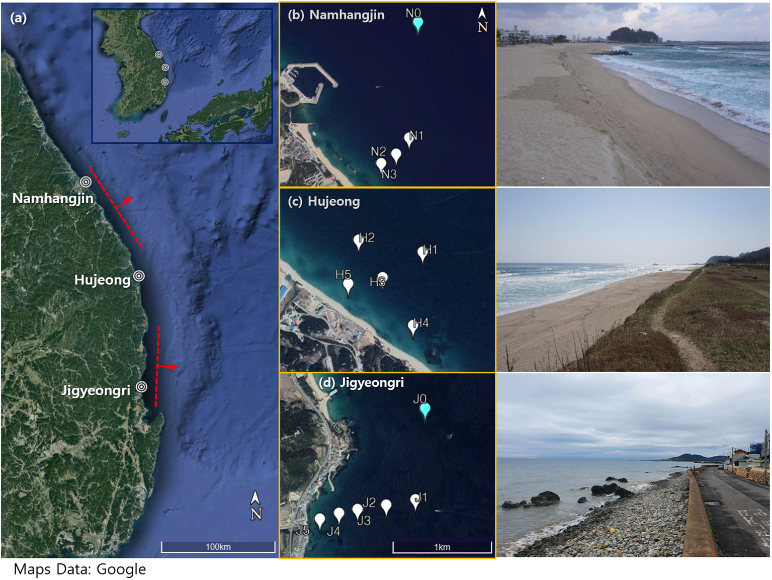
Figure 1 (A) Locations of the study sites on the east coast of Korea; (B–D) maps of observation stations at each site (left) and photographs that show the sediment conditions of the sites (right). The three sites, Namhangjin, Hujeong, and Jigyeongri, are marked as Site N, Site H, and Site J in the manuscript.

IGWs are surface gravity waves with frequencies lower than SWs, typically ranging from 20 sec to 300 sec (e.g., Oh et al., 2020). In terms of height, IGWs are only a few mm to cm high in the deep ocean (e.g., Rawat et al., 2014; Crawford et al., 2015; Smit et al., 2018) but can reach nearly 1.0 m close to shore under storm conditions (Ruessink, 2010; Fiedler et al., 2015; Inch et al., 2017; Bertin et al., 2020). Unlike SWs, which are dissipated via the breaking process in shallow water, IGWs sometimes abruptly increase near the shore (Fiedler et al., 2015; Gao et al., 2019). Researchers have reported that IGWs can cause (or at least increase) beach erosion under energetic wave conditions (Roelvink et al., 2009) and induce harbor agitation or resonance (Bellafont, 2019; Gao et al., 2020). Severe harbor resonance phenomena can further disrupt the loading/unloading operations of ports. Thus, IGWs near the coast need to be considered and studied as much as SWs.

Two mechanisms are responsible for the generation of IGWs. The group waves in SWs excite group-bound IGWs, and the bound IGWs are amplified through interactions of these SWs as the radiation stress becomes greater in a group of higher waves (Longuet-Higgins, 1962; Zhang et al., 2020). In the nearshore zone where SWs break, bound waves are released and travel in the form of free waves to the coast and are reflected, propagating toward the open ocean (Baldock, 2012; Zhang et al., 2020). Free IGWs can also be generated in the surf zone when the time-varying breaking points act as free wave generators, creating energy at infragravity frequencies (Symonds et al., 1982).

The generation and growth of IGWs are highly nonlinear processes and difficult to precisely predict closer to the shore. Nearshore IGWs are sensitive to water depth, sediment, and other geomorphological conditions, so it is difficult to consistently estimate IGWs despite their certain correlation with SWs. Steady attempts have been made to predict IGWs using the correlation between SWs and IGWs (Nelson et al., 1988; Bowers, 1992; McComb et al., 2005). Moreover, an empirical formulation for IGWs with numerically modeled ocean waves has been attempted (Ardhuin et al., 2014; Rawat et al., 2014). However, the consistency of the estimated IGW cannot be guaranteed under various conditions close to shore, so IGWs have not been treated as a major factor for coastal structural design or environmental impact analysis, even when considerable IGW impact was expected. Therefore, it would be useful for engineering applications if some practical methods to predict reliable IGW height or energy are developed; here, a reliable IGW should vary consistently with water depth and other geomorphological factors.

In this study, the dependency of IGW height on SW parameters was investigated by considering the propagation of IGWs. For this investigation, continuous observations for approximately 1 year or more were made at three different sites along the east coast of South Korea. At each site, wave gauges were deployed at different depths from an intermediate depth to the surf zone, where the correlation between SWs and IGWs was consistently observed (Herbers et al., 1995b; Ruessink, 1998; Mahmoudof et al., 2021), unlike the inside of the surf zone, where IGW transformation was significantly affected by the topography (Munk, 1949; Herbers et al., 1995a; Sheremet, 2002). Therefore, at these three sites, observing the IGW growth through a comparison of the results between the different sites is effective.

To accurately estimate IGWs, it is important to understand IGW propagation during shore-approaching processes, which is mainly affected by IGW shoaling and dissipation. The shoaling of IGWs in the nearshore zone may be more significant than the conservative SW shoaling caused by the decrease in the water depth because the IGW height can additionally increase when the energy is transferred to the IGWs from the SWs. Therefore, the rate of IGW shoaling could be higher than the conservative shoaling that follows Green’s law, by which the shoaling is proportional to $d^{-1/4}$, where $d$ is the water depth (Bertin et al., 2018). The energy transfer that contributes to IGW shoaling depends on the bed slope, as more energy can be transferred to the infragravity frequency band on a gentle slope (Henderson et al., 2006; De Bakker et al., 2015; De Bakker et al., 2016; Li et al., 2020). On steeper slopes, the energy can be transferred away from the IGW band to the SW band, thereby contributing to the reduction in IGW height (Bertin et al., 2018). Therefore, the pattern of energy transfer between SWs and IGWs should be carefully examined, specifically for shore-approaching waves. Dissipation due to bottom friction may play only a secondary role in reducing the IGW energy (Van Dongeren et al., 2007; De Bakker et al., 2014). However, it may become significant over coral reefs (Pomeroy et al., 2012; Van Dongeren et al., 2013), implying that seabed conditions can be considered factors in the development of shore-approaching IGWs (Billson et al., 2019; Poate et al., 2020).

In the present study, the IGW shoaling and dissipation processes were considered by analyzing the energy transfer and comparing the seabed conditions between the observation sites, according to the study goal of investigating the correlation between IGW and SW parameters during wave propagation to the shore. Previously, the correlation of the low-frequency band with SWs has been studied by many researchers. For example, linear dependence was observed between the IGW and SW heights (Tucker, 1950; Herbers et al., 1995a). Bowers (1992) suggested an empirical relationship for IGW height by considering additional parameters, such as the SW period and water depth. Later, Ardhuin et al. (2014) suggested a correlation, supporting the linear dependence between the IGW and SW heights and the additional dependence of $H_{IG}$, significant wave height of the IGWs, on the SW period and water depth, indicating IGW shoaling due to decreasing water depth. This correlation was used in the WAVEWATCH III spectral wave model (Tolman, 2008) to parameterize the nearshore source of IGWs as a function of the SW spectrum. In this study, however, the proportional coefficient between $H_{IG}$ and SW parameters was not closely analyzed, although its range significantly varied from one site to another. Ardhuin et al. (2014) suggested that the shelf width could be an important factor that affected the proportional coefficient.

On the other hand, some studies have reported that the IGW height is proportional to the wave energy flux instead of the SW height (Inch et al., 2017; Poate et al., 2020). For example, Inch et al. (2017) examined the correlation of the IGW height with various SW parameters, such as the SW height, period, and energy flux, and reported that the highest determination coefficient, $r^2$, of the linear regression was found in the case of the wave energy flux, as $H_{IG}\approx H_s^2$, where $H_s$ is the significant wave height of SWs. Similarly, Poate et al. (2020) examined the same correlation at two different sites on rocky platforms and observed that the slope of the regression line between $H_{IG}$ and $H_s^2$ was greater on sloping platforms than on flatter platforms, suggesting that the transformation of infragravity energy across platforms was more energetic on sloping platforms. Poate et al. (2020) further suggested that, based on their observational and modeled data, a linear parameterization of the IGW height with offshore energy flux might not always be suitable because it is highly site specific.

In this study, we compared both of the correlations suggested by Ardhuin et al. (2014) (i.e. $H_{IG}$ vs. $H_s{T}_m^2$ where $T_m$ is the mean period of SWs) and by Inch et al. (2017) (i.e. $H_{IG}$ vs. $H_s^2{T}_m$) based on the wave data sets measured at three different sites. Two of these sites are sandy beaches, and the other is basically a rocky coast covered with sediments composed of a sand and gravel mixture. The beach profiles were similar outside the surf zone. Therefore, the hydrodynamic and geographic conditions in this study were distinguished from those in previous studies, whose data were measured in dissipative sandy beaches or rocky platforms with gentle slopes. We specifically focus on the spatial variation pattern of the proportional coefficient, ${\alpha }_1$, by considering various factors, including beach slopes, seabed sediments, and SW breaking conditions. As mentioned, beach slope is an important factor for IGW development because it affects the energy transfer between SW and IGW bands. The seabed sediment condition is also an important factor, as it can affect IGW dissipation. Previously, Billson et al. (2019) observed that the ratio of infragravity swash height to SW height was higher for sandy beaches than gravel or mixed sand–gravel sites. We additionally considered the SW breaking index in analyzing the correlation pattern of the waves within the breaking regime by comparing the data measured at different depths along the cross-section at each site to examine the impact of SW breaking on IGW development. The wave measurements in this study were conducted constantly for approximately 1 to 2.5 years, and the data at each site contain seasonal wave variations/changes from mild to extreme storm waves, with heights greater than 4 m.

2 Materials and methods

2.1 Field observations

2.1.1 Study sites

In this study, three sites were selected along the east coast of South Korea, at which the wave data were measured at different depths from the shallowest 3.5 m to the deepest 33.5 m. The three sites are Namhangjin (hereafter, Site N), Hujeong (Site H), and Jigyeongri (Site J), and their locations are marked in Figure 1A. The eastern coast of South Korea, where the three sites are located, is a microtidal region where the maximum tidal range is approximately 0.3 m. Therefore, the impact of tides on IGW development might not be significant.

The seabed sediment pattern was clearly distinct between the sites, as shown in the photographs of Figures 1B, C, D. Site N and Site H were sandy beaches where berms and dunes were developed in the backshore. The sediment size was similar between the two beaches, i.e., D₅₀≈0.8~1.0 mm. In contrast, the foreshore of Site J was covered with gravels greater than 20 mm in size and partially covered with rocks. Inside the water, the seabed was largely covered by rocks, and sediments were occasionally observed over the rocks. Figure 2A shows the rocky seabed condition at $d$=5 m (J5) on 24 November 2021 when a pressure gauge was installed on a rock. The seabed sediment became finer with increasing depth, as a mixture of sand and gravel (D₅₀>100 mm) was found at $d$=24 m (J1) on the same day (Figure 2B). Outside the water, a road is parallel to the shore in the backshore area of Site J, which restricts the size of the backshore to a narrow band whose width is no greater than 5 m (Figure 1D).

FIGURE 2

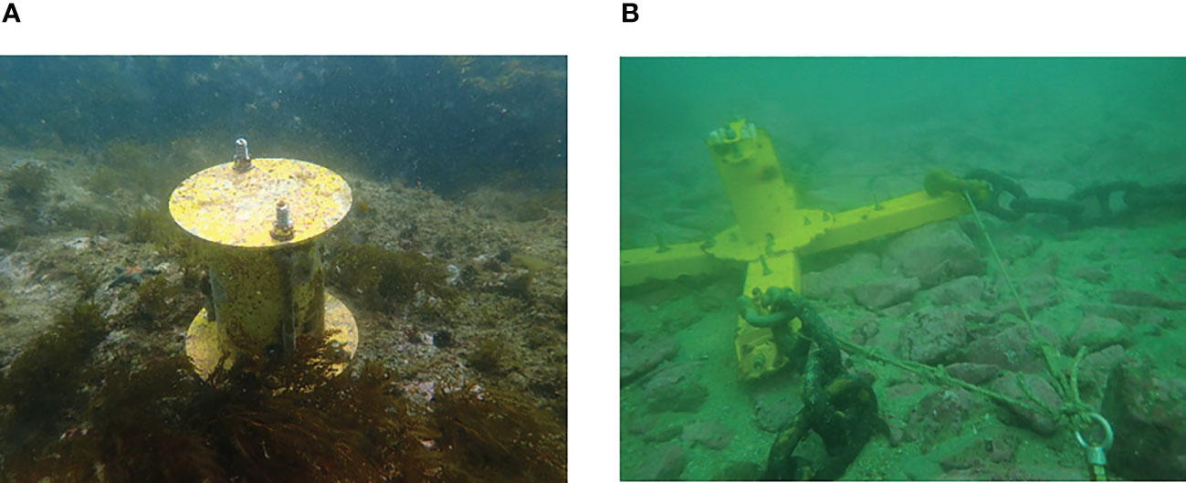
Figure 2 Photographs showing the seabed conditions at wave stations (A) J5 at $d$=5 m and (B) J1 at $d$=24 m. The photographs were taken on 24 November 2021.

The seabeds of Site N and Site H had steeper bottom slopes in the shallow areas (seabed bottom slope, $s_p$~1/12), whereas the slope became milder ($s_p$~1/40–1/50) in deeper areas (d>8 m). In between the two sites, the slope became flat (Site N), or a nearshore bar was observed (Site H), indicating that the SWs were likely breaking at depths of 5–8 m for both Site N and Site H. At Site J, the profile was monotonous compared to the sandy beaches, with a slope of 1/50. Although the slope became different in the shallow nearshore areas between the sites, it was similar outside the surf zone, as $s_p$ ranged from 1/40–1/50 at all three sites.

2.1.2 Observations

At three sites (Site N, Site H, and Site J), four to six wave gauges per site were employed to measure wave data at water depths from 3.5 m to 33.5 m for 11–31 months (the details are listed in Table 1). At Site N, four pressure transducers (PTs) were deployed at the wave stations from N0 to N3, as shown in Figure 1B. The depths of each station were 31 m (N0), 14 m (N1), 10 m (N2), and 6 m (N3), and the wave data were measured for 22 months from 1 Feb. 2013 to 10 Dec. 2014. In addition, a Nortek Acoustic Wave and Current profiler (AWAC) was installed at the same location of N0 ($d$=31 m) to validate the PT data. An array of three stations from N1 to N3 was formed in the perpendicular direction to the shoreline, whereas N0 was located separately offshore of the breakwater that was constructed to protect the shore and the port near Namhangjin. At Site H, PTs were installed at five stations at depths of 19 m (H1), 14 m (H2), 9 m (H3), 5 m (H4), and 3.5 m (H5), as marked in Figure 1C. The PTs were deployed between 2008 and 2020. It should be noted that, however, the times of wave measurements were different between the stations at Site H (each observation period is described in Table 1), indicating that direct comparisons during concurrent wave conditions were not available at this site. However, comparisons of the wave statistics were still valid between different depths at the site and with those at other sites. At Site J, an array of five PTs was deployed at six stations at depths of 24 m (J1), 19 m (J2), 12 m (J3), 8 m (J4), and 5 m (J5) from 11 Sep. 2021 to 29 Sep. 2022 (Figure 1D). At J0 ($d$=33.5 m), in addition to a PT, an AWAC was installed for the validation of wave measurements during the same period. Stations installed with an AWAC at depths deeper than 30 m, such as N0 and J0, were specifically marked with ‘0’ to distinguish them from the stations where only PTs were installed. For example, all the stations at Site H had only PTs at water depths shallower than 30 m, and there was no H0 station. The observation period was different between the wave stations, but their data were constantly measured during the observation period of each station. The observation periods listed in Table 1 show that the shortest duration of wave measurements was 11 months at station H4, and the longest duration was 31 months at H1. Therefore, the wave data used in this study can represent the wave climates at the three sites, reflecting their seasonal changes. For example, the energetic wave conditions during the typhoon seasons in late summer and early autumn and during the winter storm seasons were reflected in the observation data sets.

TABLE 1

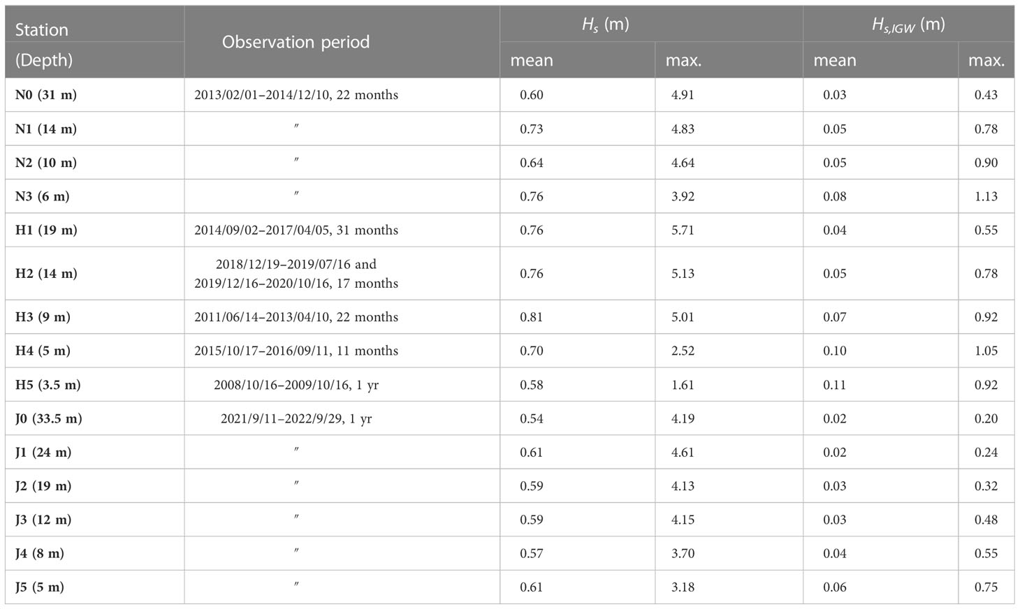
Table 1 List of the water depths ($d$), observation periods, and mean/maximum wave heights at each wave station.

2.2 Methodology

2.2.1 Previous study results

As described in the introduction, the goal of this study is to compare the dependency of the IGW height on the short-wave parameters with the previous studies by Ardhuin et al. (2014) and Inch et al. (2017). In this section, the parameterization by the previous studies are described.

Before Ardhuin et al. (2014), linear dependence was observed between the IGW and SW heights (Tucker, 1950; Herbers et al., 1995a). Similarly, Bowers (1992) suggested an empirical relationship for IGW height by considering additional parameters, such as the SW period and water depth, as

$\begin{array}{ll}{H}_{IG}\approx H_s^{\beta }{T}_p^{\gamma }{d}^{\delta }& (1)\end{array}$

where $T_p$ is the peak period of SWs; and $d$ is the water depth. In this study, 1.32, 1.17, and -0.34 were used for $\beta$, $\gamma$, and $\delta$, respectively, to minimize scatter in the data plot, using the field data measured in Port Talbot, United Kingdom. Later, Ardhuin et al. (2014) used data sets obtained from North Carolina and Hawaii (United States) and Crozon, Bertheaume, and Banneg island (France) and suggested a correlation,

$\begin{array}{ll}{H}_{IG}\simeq {\alpha }_1{H}_s{T}_m^2\sqrt{g/d}& (2)\end{array}$

where $T_m$ is the mean period of SWs, $g$ is the acceleration of gravity, and ${\alpha }_1$ is a proportional coefficient. This correlation supports the linear dependence between the IGW and SW heights and the additional dependence of $H_{IG}$ on the SW period and water depth, indicating IGW shoaling due to decreasing water depth.

Inch et al. (2017) reported that the IGW height was more closely related to the short wave energy flux, rather than the SW height, suggesting a correlation as

$\begin{array}{ll}{H}_{IG}\approx H_o^2{T}_p& (3)\end{array}$

where $H_o$ is the offshore SW height and $T_p$ is the peak wave period, which was also supported by Poate et al. (2020) although the IGW height dependency on offshore energy flux might be highly site specific.

2.2.2 Wave measurement and analysis

The AWAC measures the surface elevation by acoustic surface tracking (AST) with vertical beams. The AWAC for this study recorded 2048 samples (≈17.1 min) at a rate of 2 Hz every 30 min. Then, the surface elevation spectrum $E(f)$ was estimated from the AWAC-obtained surface elevation. On the other hand, the surface elevation data from the PT were estimated from simultaneous subsurface pressure data at a 2 Hz sampling rate. In this study, subsurface pressure signals of 8192 samples (≈68.3 min) were transformed into surface elevation spectra by the power spectrum density of wave pressure $E_p(f)$, which was obtained from the hydrostatic elevation by Fourier transform. The hydrostatic elevation $\zeta$ was converted from the pressure gauge signal $P$ by considering atmospheric pressure, with the density of water ${\rho }_w$, the gravitational acceleration $g$ and the mean water depth $d$.

$\begin{array}{ll}\zeta =\frac{P}{{\rho }_{w}g}-d& (4)\end{array}$

Then, the surface elevation spectrum $E(f)$ was obtained from the wave pressure spectrum $E_p(f)$ and the pressure transfer function $K_p$ (Vasan et al., 2017). Here, the wavenumber $k(f)$ was obtained from the linear dispersion relationship that assumes the small amplitude wave theory.

$\begin{array}{ll}E(f)=K_p^2{E}_p(f)& (5)\end{array}$

$\begin{array}{ll}{K}_p=\frac{\text{cosh}\left\{(d+\delta )k(f)\right\}}{\text{cosh}\left\{\delta k(f)\right\}}& (6)\end{array}$

The significant wave height $H_s$ or the mean period $T_m$ of SWs can be estimated from the surface elevation spectrum $E(f)$ by using spectral moments in Eqn. (7) (Holthuijsen, 2007). The nth-order spectrum moment $m_{\text{n}}$ was calculated as in Eqn. (8) with the upper and lower limits $f_{\text{upper}}$ and $f_{\text{lower}}$ of the specified frequency band of SWs. $H_{\text{s}}=4\sqrt{m_0}$,

$\begin{array}{ll}{H}_s=4\sqrt{m_0},T_m=\sqrt{m_0/m_2}& (7)\end{array}$

$\begin{array}{ll}{m}_n={\int }_{f_{\text{lower}}}^{f_{\text{upper}}}{f}^n\cdot E(f)df& (8)\end{array}$

Spectral analysis was also applied to obtain the significant wave height of IGWs $H_{s,\text{IGW}}$ using the IGW frequency band. The upper limit of the SW frequency band was set to 0.3 Hz, and the lower limit of the IGW frequency band was set to 0.004 Hz. The upper limit of the IGW frequency band and the lower limit of the SW frequency band were set equal to 0.05 Hz.

$\begin{array}{ll}{H}_{\text{s},\text{IGW}}=4\sqrt{m_{0,\text{IGW}}}& (9)\end{array}$

$\begin{array}{ll}{m}_{n,\text{IGW}}={\int }_{f_{\text{lower},\text{IGW}}}^{f_{\text{upper},\text{IGW}}}{f}^n\cdot E(f)df& (10)\end{array}$

Bispectral analysis was performed to examine the nonlinear energy transfer between SWs and IGWs. The bispectrum $B_{f_1,f_2}$ represents the coupling between $f_1$, $f_2$ and $f_1+f_2$ and indicates whether or not there is a triad nonlinear interaction (Hasselmann et al., 1963; Elgar and Guza, 1985).

$\begin{array}{ll}{B}_{f_1,f_2}=\text{E}[A_{f_1}{A}_{f_2}{A}_{f_1+f_2}^{*}]& (11)\end{array}$

where $A_{f_n}$ is the complex Fourier coefficient at frequency $f_n$ ($n=1,2$), and $\text{E}[]$ is the ensemble average operator for the product of $A_{f_1}{A}_{f_2}$ and the complex conjugate term $A_{f_1+f_2}^{*}$. The imaginary part of the bispectrum indicates the direction and magnitude of the energy transfer between the frequency components $f_1,f_2$ (Herbers et al., 2000). Positive values of the imaginary part of $B_{f_1,f_2}$ indicate energy transfer from $f_1$ and $f_2$ to $f_1+f_2$. Negative values of the imaginary part of $B_{f_1,f_2}$ indicate energy transfer from $f_1+f_2$ to $f_1$ and $f_2$.

3 Data

AWAC data measured at N0 and J0 for validation of PT data had good correlations with PT data, as their correlation coefficients between the $H_s$ of AWAC and PT data are 0.96 at N0 and 0.95 at J0, supporting the accuracy of the PT measurements, even at the deepest stations. Furthermore, the AWAC could provide wave-directional information at the two sites. The principal directions of wave propagations were NE and ENE, as 25–30% of the waves came from the NE for both stations. Although AWACs were not installed at Site H, its primary wave direction may also be NE, as previously observed (Chang et al., 2019; Do et al., 2021).

In Table 1, the mean and maximum values of SW and IGW heights are listed, as they were measured during the whole observation period of each wave station. Because the observation periods were different between the sites, a direct comparison is not feasible. However, the wave conditions were comparable between the three sites. At Site N, the mean values of the significant wave height of SWs ($H_s$) varied from 0.60 m to 0.76 m, showing a shoaling pattern as the measured depth decreased from 31 m (N0) to 6 m (N3). In contrast, the maximum values decreased with decreasing depth from 4.91 m (N0) to 3.92 m (N3), likely due to the effect of SW breaking. This pattern was similarly observed at Site H and Site J, as their maximum values decreased with decreasing depth. In terms of the mean values, however, Site H showed a difference from the patterns in Site N and Site J, as SW shoaling was not clearly observed, likely because the wave stations in Site H were not aligned and refraction conditions changed.

In the case of the IGWs, the shoaling pattern was clearly observed as both the mean and maximum values of the significant wave height ($H_{s,IGW}$) increased as the water depth decreased. In particular, the maximum values of $H_{s,IGW}$ significantly increased as the waves approached the shore. At Site N, its maximum value was 0.43 m at $d$=31 m (N0) but reached 1.13 m at $d$=6 m (N3). The high values of the IGW height (>1 m) were not extraordinary in this study, as was also observed in previous studies (Ruessink, 2010; Fiedler et al., 2015; Inch et al., 2017; Bertin et al., 2020). At Site H and Site J, the shoaling pattern of IGWs was also clearly observed, as the maximum values of $H_{s,IGW}$ were measured to be 1.05 m and 0.75 m at $d$=5 m at Site H and Site J, respectively. At Site H, the maximum value of $H_{s,IGW}$ decreased to 0.92 m at $d$=3.5 m, possibly due to IGW dissipation. However, this result cannot be confirmed because a direct comparison was not feasible between the wave stations at Site H, as their observation periods were different, as listed in Table 1.

In Figure 3, time variations in $H_s$ are compared between the wave stations at Site H and Site J for the selected wave events measured in February 2013 and September 2021. The two wave events were selected because they can represent the irregular pattern of SW shoaling at the study sites. In Figure 3A, shoaling was observed only at some specific times during the whole event period of ~2.5 days. For example, shoaling was clearly observed during the growth (03:00–9:00, 15 February 2013)/decay (06:00–17:00, 16 February 2013) phases of $H_s$ and at the phase of the $H_s$ peak (15:00–21:00, 15 February 2013). The pattern of shoaling was, however, different between the phases because the decrease in $H_s$ was clearly observed only between N0 ($d$=31 m) and N1 ($d$=14 m) in the growth/decay phases, whereas it was dominant between N1 and N2 ($d$=10 m) during the peak phase. Between N2 and N3 ($d$=6 m), the changes in $H_s$ were minimal in all three phases. The irregular shoaling pattern was also observed at Site J. Figure 3B clearly shows that $H_s$ increased between J0 ($d$=33.5 m) and J1 ($d$=24 m). At shallower depths, however, the shoaling of SWs is not clearly distinguishable between stations J1 to J5. Similar to the cases in Figure 3, SW shoaling occurred only irregularly or was not clearly observed in many other cases during the experimental periods. The irregularity in the SW shoaling pattern was also observed in the statistics listed in Table 1. In contrast, the table shows that shoaling was clearly observed in the case of IGWs. The data at Site H were not included, as the comparison was not feasible due to the different observation times between the stations. The data used to produce the figures in this study are available in Mendeley (Oh and Jeong, 2023).

FIGURE 3

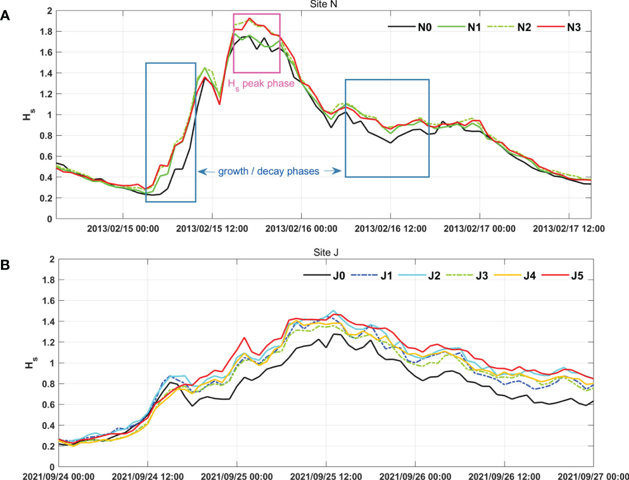
Figure 3 Time variations in $H_s$ during selected wave events that represented the irregular pattern of SW shoaling at (A) Site N from 15 February 2013 to 17 February 2013 and (B) Site J from 24 September 2021 to 27 September 2021. The data at Site H are not presented due to the absence of concurrent station data.

4 Results

4.1 Correlation of IGW height with SW parameters

In this section, the correlations between the significant wave height of IGWs ($H_{s,IGW}$) and SW parameters are investigated. Two types of SW parameters, $H_s^2*T_m$ and $H_s*T_m^2$, were examined because they were suggested in previous studies by Ardhuin et al. (2014) and Inch et al. (2017), respectively, as described in Section 1. Before testing these parameters, the direct relationship between the SW height, $H_s$, and IGW height, $H_{s,IGW}$, was examined because a linear dependency between the two wave heights was observed in Herbers et al. (1995b). In Figure 4, the correlations were estimated using the wave measurements from all observation periods at all wave stations at the three sites. Each data point was calculated from the wave spectra obtained by measuring waves for up to ~68.3 min every hour during the observation periods, as described in Section 2.2. The figure shows strong correlations between them, as $H_{s,IGW}$ increases with $H_s$ at all wave stations. However, it does not confirm a linear dependency because the data were widely scattered around the regression lines. In particular, the correlation pattern became more quadratic as the water depth decreased. In the case of Site N, for example, the data were scattered around the linear regression lines (black solid lines), with a coefficient of determination of $R^2$=0.86 at the deepest wave station ($d$=31 m). The scattering became narrower as the water depth decreased. However, $H_{s,IGW}$ significantly increased over a similar range of $H_s$, which makes the regression pattern more quadratic. This pattern of narrower scattering but deviation from the linear regression with decreasing water depth was similarly observed at the other two sites: Site H and Site J. The colors of the scattered data points denote the breaker ratio ($H_s/d$) as an index of SW breaking. For example, the yellow to red colored dots mark the data that belong to the breaking regime, which was determined using a simple conventional SW breaking index ($H_s/d<$ 0.33). Therefore, the results in Figure 4 indicate that linear correlation might not be applicable for the SW and IGW heights, specifically in the surf zone.

FIGURE 4

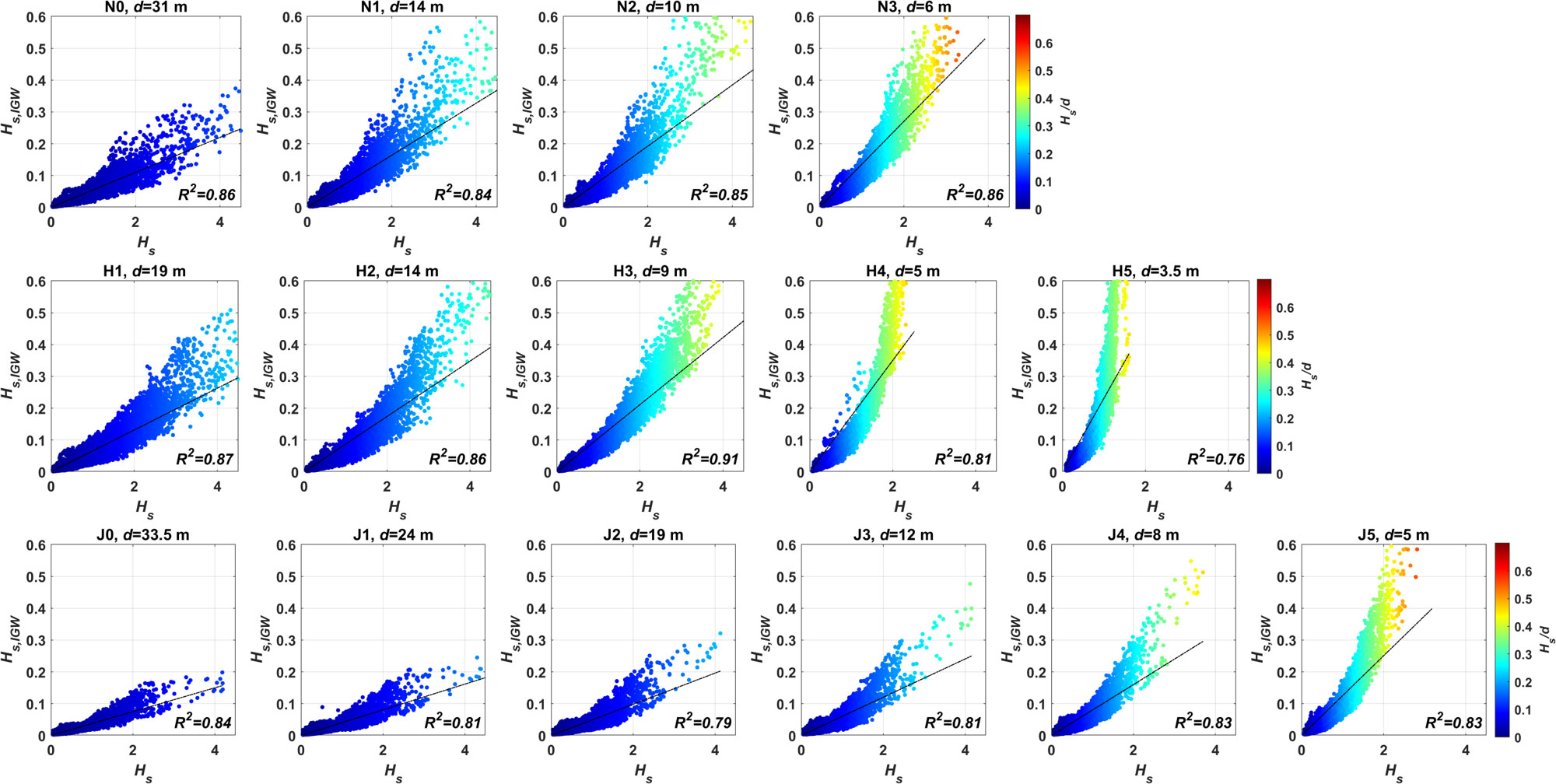
Figure 4 Correlations of the significant wave heights between SWs ($H_s$) and IGWs ($H_{s, IGW}$). Top panels: N0–N3; middle panels: H1–H5; bottom panels: J0–J5. The ‘0’s used to mark the wave stations distinguish the wave stations with AWACs from the stations with PTs, in which numbers (1, 2, 3, …) mark the deeper wave stations. The black solid lines are the linear regressions. The regression coefficients, $r^2$, are also marked for each wave station.

The quadratic correlations in Figure 4 indicate that the shoaling rate of $H_{s,IGW}$ was greater than that of $H_s$, which was also suggested by the data in Table 1. In Figure 5, the pattern of wave height changes during the shore-approaching process is compared between SWs and IGWs, in which the estimated values of $H_s$ and $H_{s,IGW}$ of selected wave events are plotted against different water depths. The data were selected at concurrent times at all the wave stations at each site so that the spatial variation in wave heights could be directly compared during the same courses of propagation. In addition, the selection of wave events was necessary because the mean values of all wave data would smear the plots, and the shoaling pattern could not be identified. For example, Figures 5A, B show the statistics of the waves whose $H_s$ values were greater than 2 m. For those energetic waves, the shoaling of SWs was not clearly observed along the shore-approaching courses. In fact, the $H_s$ of Site J decreased at the shallowest water depth, which was an indication of SW breaking. In contrast, IGW shoaling was clearly observed at both sites, as the mean values of $H_{s,IGW}$ increased to 0.4 m at the shallowest water depths, whereas they were lower than 0.2 m at the deepest stations. Figures 5C, D show the same statistics as those in Figures 5A, B, but for the specifically selected wave events during which the shoaling of SWs was detectible from the comparison of time series data between the wave stations, and examples are shown in Figure 3. In this case, the SW shoaling pattern became more obvious than those in Figures 5A, B, and IGW shoaling was more clearly observed. These results confirm those found in Table 1 and Figure 4 that shoaling occurred more dominantly for IGWs than SWs. Note that the data from Site H are not included in Figure 5 because the comparison during wave propagation was not available due to the different observation times between the stations.

FIGURE 5

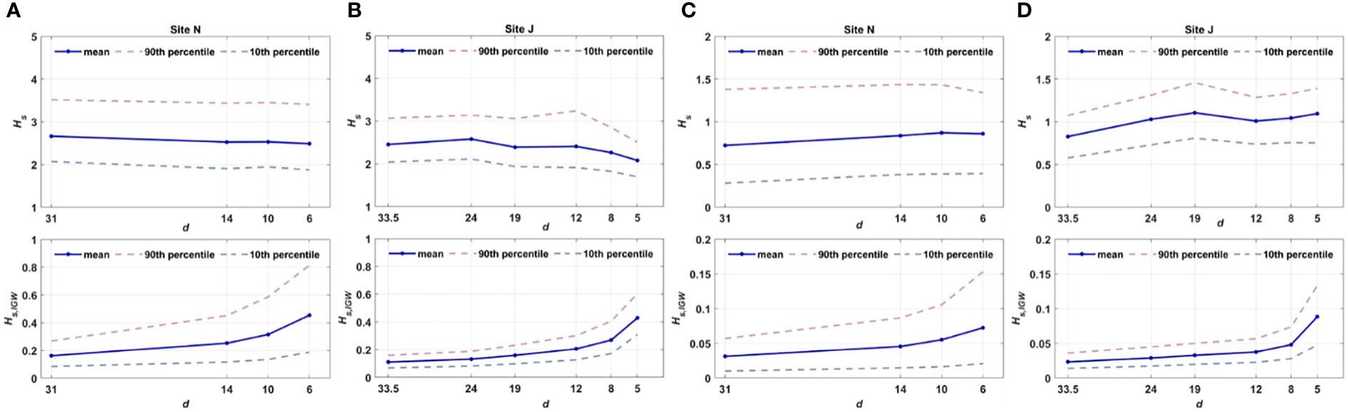
Figure 5 Comparison of the spatial variations in the $H_s$ and $H_{s,IGW}$ of selected wave events during shore-approaching courses. (A) Upper panel: mean values (blue solid line) of $H_s$ of the wave events selected only when $H_s$ was greater than 2 m at Site N; lower panel: $H_{s,IGW}$ of the same wave events used in the upper panel; (B) same as Aa) but for Site J; (C) upper panel: mean values (blue solid line) of $H_s$ of the wave events during which SW shoaling was detectible (as shown in Figure 3) at Site N; lower panel: $H_{s,IGW}$ of the same waves used in the upper panel; (D) same as (C) but for Site J The pink and gray dashed lines represent the 90th and 10th percentiles of the selected wave events for each panel, respectively.

An increase in IGW energy was also detected via the comparative view of the power spectra. Figure 6 compares the power spectra measured at different depths between Site N and Site J. To examine the spatial variation in the spectra during wave propagation, the data at different wave stations were measured at concurrent times for each station. For Site N, the spectra were constructed based on the wave data measured over 5 hours from 2:00 to 7:00 on 7 Apr. 2013 and over 6 hours from 9:00 to 15:00 on 19 Sep. 2022 for Site J. In addition, the specific times were selected for Site N and Site J because the $H_s$ was greater than 4 m during the times when the spectra were estimated. The energetic wave conditions were used for the comparison because the difference between the wave stations was clearly reflected in the power spectra. The data at Site H are not included in Figure 6 because a direct comparison among stations cannot be made due to the absence of concurrent station data.

FIGURE 6

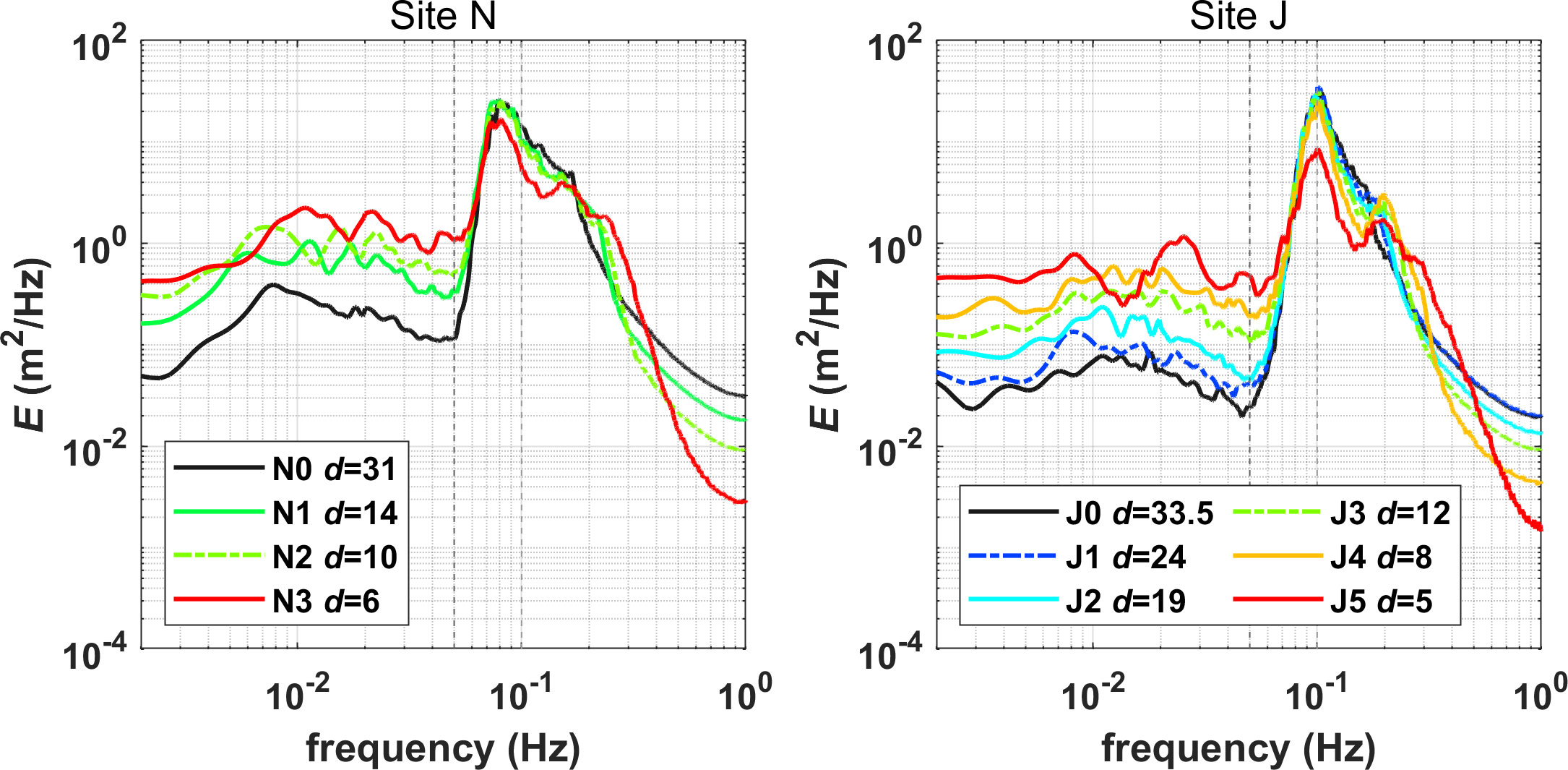
Figure 6 Comparison of power spectra between Site N and Site J. The spectra were calculated from measured data at 2:00 to 7:00 on 7 Apr. 2013 and at 9:00 to 15:00 on 19 Sep. 2022 for Site N and Site J, respectively, during which the incident wave heights were greater than 4 m.

Figure 6 shows that two patterns are consistently observed in the power spectra of the two sites. First, there are SW frequency bands in which the spectrum magnitude (i.e., SW energy) decreases with decreasing water depth. In the case of Site N, for example, the peak of SWs is found at $f_p$≈0.08 Hz (=12.5 s), and the spectrum magnitude sharply decreases to the higher and lower frequencies. In particular, the level of the spectrum magnitude decreases as the water depth decreases within the SW frequency band from 0.05 Hz (=20 s) to 0.15 Hz (≈6.7 s). Although $f_p$ is different for the other two sites, this pattern of SW energy decrease with decreasing water depth is observed at both sites. Second, the level of spectral magnitude in the IGW frequency band increases with decreasing depth. However, the energy magnitude of the spectra in the IGW band is different between the sites. At Site N, for example, the IGW energy was 0.12–0.37 m²/Hz at $d$=31 m and 0.80–2.20 m²/Hz at $d$=6 m, whereas it was 0.02–0.08 m²/Hz at $d$=33.5 m and 0.27–1.12 m²/Hz at $d$=5 m at Site J. The SW energy decrease and IGW increase with decreasing water depth in Figure 6 support the observations in Figures 4, 5, as they both indicate that IGW shoaling is greater than that of SWs. The discrepancy between SW and IGW development is further analyzed in Section 4.3 with a discussion of energy transfer.

In Figures 7, 8, the correlation between IGWs and SWs is examined using two parameters, i.e., $H_s*T_m^2$ and $H_s^2*T_m$, using the same data sets in Figure 4, based on all wave measurements available at the three sites. The results show a largely linear correlation of $H_{s,IGW}$ with both of the parameters. Therefore, linear regression lines can be estimated as they fit the scatterplots with $H_{s,IGW}=A_1*H_s*T_m^2$ and $H_{s,IGW}=A_2*H_s^2*T_m$, where $A_1$ and $A_2$ are the proportional coefficients for the data in Figures 7 and 8, respectively. Although the linear fits reasonably represent the correlations between the SWs and IGWs in both figures, their regression pattern is distinct. One way to quantify the regression pattern is to estimate the coefficients of determination, $R^2$, as listed in Table 2. For $H_s*T_m^2$, $R^2$ values are higher than 0.95 for the wave stations that are deeper than 10 m and decrease at the shallower stations, as the lowest $R^2$ value is observed to be 0.82 at the station with a depth of 5 m (H4). Because the high $R^2$ values denote that the linear regression lines nicely represent the scattered data, the lower $R^2$ values at the shallower depths indicate that the data are poorly represented by the linear fits. The scatterplots in Figure 7 also confirm the $R^2$ values, as the correlation pattern becomes more quadratic at shallower depths ($d$<10 m), whereas it corresponds to a linear regression better at deeper stations.

FIGURE 7

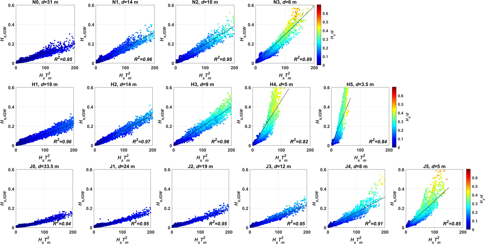
Figure 7 Correlations of $H_{s, IGW}$ with the SW parameter, $H_s{T}_m^2$. Top panels: N0–N3; middle panels: H1–H5; bottom panels: J0–J5. The black solid lines are the linear regressions. The regression coefficients, $R^2$, are also marked for each wave station.

FIGURE 8

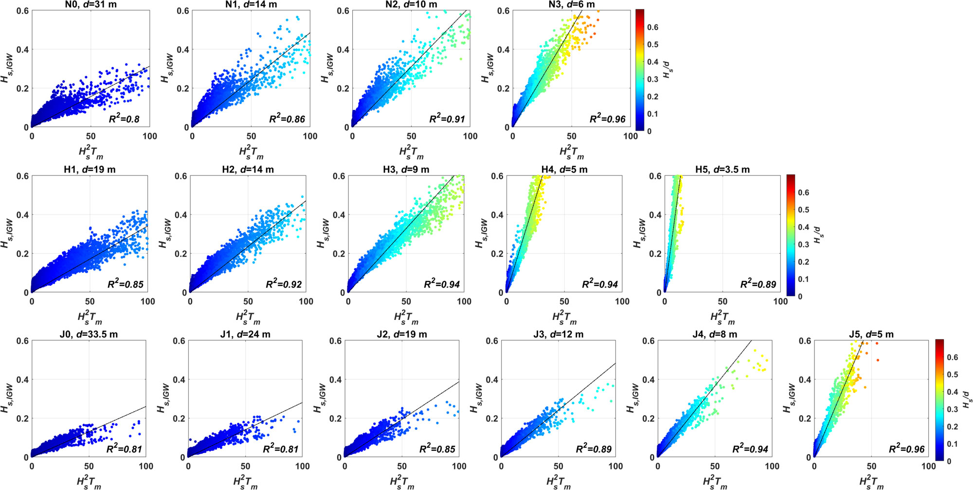
Figure 8 Correlations of $H_{s, IGW}$ with the SW parameter, $H_s^2{T}_m$. Top panels: N0–N3; middle panels: H1–H5; bottom panels: J0–J5. The black solid lines are the linear regressions. The regression coefficients, $R^2$, are also marked for each wave station.

TABLE 2

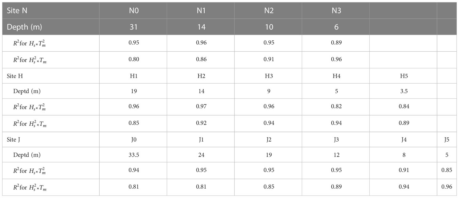
Table 2 List of coefficients of determination, $R^2$, for each wave station at the three sites for the regression comparison between the two SW parameters: $H_s*T_m^2$ and $H_s^2*T_m$.

The yellowish or reddish colors of the scattered data observed at the wave stations shallower than 10 m in Figure 7 indicate that the corresponding wave conditions belong to the SW breaking criteria, as $H_s/d$ is smaller than 0.33. Note that these yellowish or reddish data points are mostly located along the upper parts of the regression lines, as they contribute to the quadratic pattern of the correlations. Therefore, the deviation of the IGW correlation from the linear regression at shallower depths may be due to SW breaking. $H_{s,IGW}$ shows linear dependence on $H_s*T_m^2$ for the waves in the nonbreaking criteria, but the linearity becomes weaker with the addition of the data in the breaking criteria.

The correlations of $H_{s,IGW}$ with the wave energy flux, $H_s^2*T_m$, clearly show different patterns from those with $H_s*T_m^2$. Figure 8 shows the scatterplots between the two SW and IGW parameters with the linear regression lines (black solid lines), $H_{s,IGW}=A_2*H_s^2*T_m$. One of the significant characteristics of the regression pattern with the energy flux is that the $R^2$ values are lower at the deeper wave stations but increase with decreasing depth, which is opposite to the pattern of $H_s*T_m^2$. The data in Figure 8 show that the scatterplots were concentrated along the upper parts of the regression lines at the wave station deeper than 10 m, which makes the scatterplots concave down, lowering the $R^2$ values. As the water depth increases ($d$<10 m), however, the data are better fit by a linear regression, with $R^2$ values higher than 0.94, except for the data at the shallowest station, H5 ($d$= 3.5 m). The opposite trend of the spatial variation in $R^2$ values between Figures 7 and 8 indicates that the accuracy of regression analysis strongly depends on the water depth, although the correlations of IGW height show largely linear dependence with both SW parameters.

4.2 Linear regression coefficients

The correlation results in Figures 7 and 8 indicate that the slope of the linear regression lines increased as the water depth decreased, which means that the proportional coefficients, $A_1$ and $A_2$, in the two correlations, $H_{s,IGW}=A_1*H_s*T_m^2$ and $H_{s,IGW}=A_2*H_s^2*T_m$, might be depth dependent. In previous studies, water depth was already considered a controlling factor, as an empirical relationship, i.e., $H_{IG}\approx H_s^{\beta }{T}_p^{\gamma }{d}^{\delta }$, was suggested (Bowers, 1992). In that study, $\text{δ}$ was found to be -0.32 based on field measurements in Port Talbot, United Kingdom. Later, $\text{δ}$ was suggested to be -0.5 with the correlation $H_{IG}\simeq {\alpha }_1{H}_s{T}_m^2\sqrt{g/d}$ based on field data from three sites in the United States and France (Ardhuin et al., 2014). However, the proportional coefficient, ${\alpha }_1$, varied between the sites, and a representative value that could be applied to all three sites was not found.

In this section, the water depth-dependency of the proportional coefficients, $A_1$ and $A_2$, are examined for the two linear correlations, namely, $H_{s,IGW}=A_1*H_s*T_m^2$ and $H_{s,IGW}=A_2*H_s^2*T_m$, observed in Figures 7 and 8. In Figure 9A, the spatial variation in the $A_1$ values is plotted, as it is estimated from the linear correlations. The x-axis of Figure 9A is the water depth expressed on the logarithmic scale, and the y-axis shows the $A_1$ values on the linear scale. The triangles in the figure denote the $R^2$ values listed in Table 2. As expected, $A_1$ is strongly dependent on the water depth, as it increases with decreasing $d$, and the increasing rate also increases with decreasing depth, showing logarithmic patterns. However, its variation pattern is distinct between the sites. Although the water depths of the wave stations are not the same, it is not easy to clearly distinguish the patterns of the different sites, and the rate of $A_1$ variation at Site N is separated from those at Site H and Site J, whereas its pattern is similar between them. It is noted that the $A_1$ values at Site N are mostly smaller than those at Site H and Site J, and its increasing rate with decreasing depth is also lower than those at the other two sites. Therefore, it is not feasible to establish a depth-dependent formula for $A_1$ that represents all three sites.

FIGURE 9

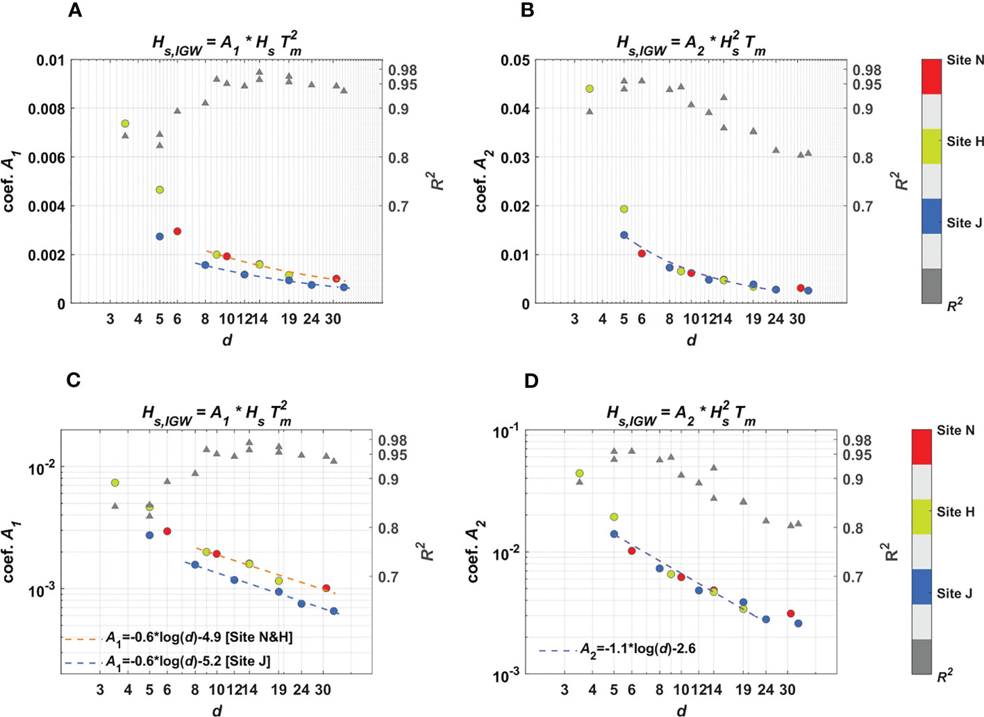
Figure 9 Depth-dependent variation in $A_1$ and $A_2$, as they are the proportional coefficients of the two correlations: $H_{s,IGW}=A_1*H_s*T_m^2$ and $H_{s,IGW}=A_2*H_s^2*T_m$. (A) $A_1$ and (B) $A_2$, plotted on the logarithmic x-scale and linear y-scale; (C) $A_1$ and (D) $A_2$, plotted on the logarithmic x-scale and logarithmic y-scale. Circles: magnitudes of $A_1$ and $A_2$, with red colors for Site N, light green colors for Site H, and blue colors for Site (J) The gray triangles denote the coefficient of determination, $R^2$, values.

The discrepancy of the variation in the proportional coefficient is greatly reduced when the wave energy flux, $H_s^2*T_m$, is considered as the SW parameter. Figure 9B shows the spatial variation in the coefficient, $A_2$, as observed in Figure 8. Interestingly, the pattern of variation becomes more consistent compared to that of $A_1$, as the spatial variation rates of $A_2$ are similar between all three sites, which implies that a representative formula for these sites can be established. There are exceptions observed at the shallow-water depths, as the $A_2$ values at $d$=3.5 m of Site H are too high to be counted in the representative pattern. Considering the shallowness of the water depths at these stations, however, these extreme $A_2$ values could be affected by the SW breaking that can change the variation pattern, and they may need to be excluded in developing the representative formula.

The consistency (or inconsistency) of the spatial variation pattern of the proportional coefficients can be more closely examined by plotting $A_1$ and $A_2$ on the logarithmic scale. In Figure 9C, the spatial variation pattern forms lines in the logarithmic domain, and the slopes of these lines are similar for all three sites. However, the discrepancy in the $A_1$ variation pattern is clearly observed, as the magnitude of $A_1$ in Site J is lower than those in Site N and Site H. The $A_1$ magnitude is similar between Site H and Site J. Based on these results, therefore, it is not easy to determine a depth-dependent $A_1$ formula that can be applied to all three sites, whereas they can be developed separately for Site N and Site H/Site J, which is not recommended considering the purpose of this study. The reason for this discrepancy is not clearly understood from the conditions at the experimental sites. The wave conditions were comparable between the sites, and the beach profile slopes were also similar. One difference between the sites can be found in the seabed conditions. As shown in Figure 2, Site N and Site H are sandy beaches, but rocky seabed conditions are observed at Site J. Previously, it was observed that the ratio of infragravity swash height to SW height was higher for sandy beaches than gravel or mixed sand–gravel sites (Billson et al., 2019); this finding corresponds to the results in Figure 9C because the $A_1$ values are higher for the sandy beaches of Site N and Site H than the rocky beach of Site J, implying that the IGW height is relatively high at Site N and Site H considering the comparable SW energy.

However, this discrepancy in the proportional coefficient disappears if the wave energy flux is considered for the SW parameter. Figure 9D, which is the representation of Figure 9B on the logarithmic scale of the y-axis, shows the $A_2$ (the proportional coefficients of $H_{s,IGW}$ to $H_s^2*T_m$) variation with depth. Except for the data measured at the shallowest depth of 3.5 m (H5) and the two depths over 30 m (N3, J5), all the $A_2$ values of the three sites are aligned and thus can be fitted into a formula, which is depth-dependent and expressed in the form of $\log (A_2)=C_1*\log (d)+C_2$. Based on the data in Figure 9D, the corresponding coefficients, $C_1$ and $C_2$, are determined to be -1.1 and -2.6, respectively, and these values can be applied for all three experimental sites of this study. However, note that the coefficient of determination, $R^2$, of $A_2$ drops below 0.85 for the deep-water data (d>10 m), whereas it remains higher than 0.94 for the shallow-water data (5 m≤ $d$<10 m), which lowers the credibility of the suggested formula, specifically for the deeper areas. In addition, note that this pattern is the opposite in the case of $A_1$, as shown in Figure 9C, because $R^2$ is higher than 0.95 for the deep-water data (d>10 m), whereas it drops below 0.9 in shallow areas ($d$<6 m). The reason for this discrepancy between the two SW parameters is not clearly understood based on the current data sets available in this study. Regardless of the discrepancies between the two different SW parameters, it is obvious that the magnitude of the proportional coefficients of the linear regressions between IGWs and SWs increased as the water depth decreased, supporting IGW shoaling in the nearshore zones, which is further discussed in the next section.

4.3 Energy transfer

In this section, the dependency of the proportional coefficients, $A_1$ and $A_2$, shown in Figure 9, are examined in terms of the energy transfer. The interaction between SWs and IGWs may be responsible for IGW shoaling because SW energy can be transferred to IGWs, causing additional IGW shoaling on gentle slopes (1/35–1/80), whereas it can be transferred back to SW frequencies on steep slopes (De Bakker et al., 2015; Bertin et al., 2018). The slopes of the three experimental sites in this study range from 1/40–1/50 in the outer regions of the nearshore sandbars, so they belong to the gentle slope regime. The results in Figures 4, 5 also support the findings in previous studies, as the shoaling of IGWs dominated at the study sites.

Figures 10–12 show the power spectra (upper panels) and the imaginary parts of the bispectra (lower panels) estimated at the wave stations of the three sites. In particular, the data at Sites N and J were measured simultaneously for each site so that the energy transfer pattern during the shore-approaching processes could be investigated. These simultaneous data were selected from the high-energy wave condition data used for the power spectra in Figure 6, as their data collection times are 3:00 on 7 Apr. 2013 and 15:00 on 19 Sep. 2022 for Site N and J, respectively. For Site H, the data were selected at different times between the stations, considering the wave conditions such that the wave height was greater than 4 m at each station (Figure 11). Therefore, the wave conditions used to build the bispectra at Site H were comparable to those at the other two sites. The imaginary parts of all bispectra are contoured from positive yellow to negative blue.

FIGURE 10

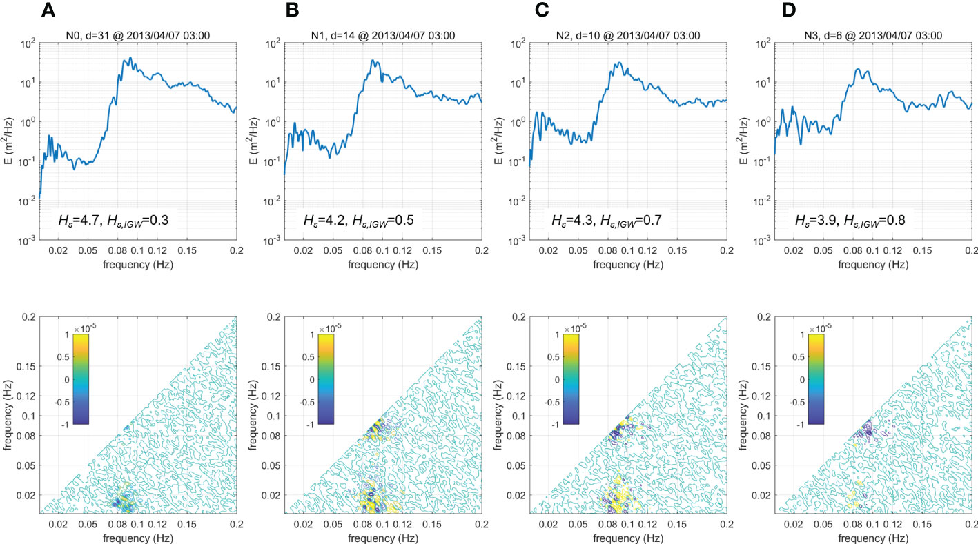
Figure 10 Imaginary parts of the bispectra (lower panels) at (A) N0, (B) N1, (C) N2, and (D) N3, with corresponding power spectra in the upper panels. The color bars in the lower panels show the color of the imaginary part values. The wave data were measured at 3:00 on 7 Apr. 2013.

FIGURE 11

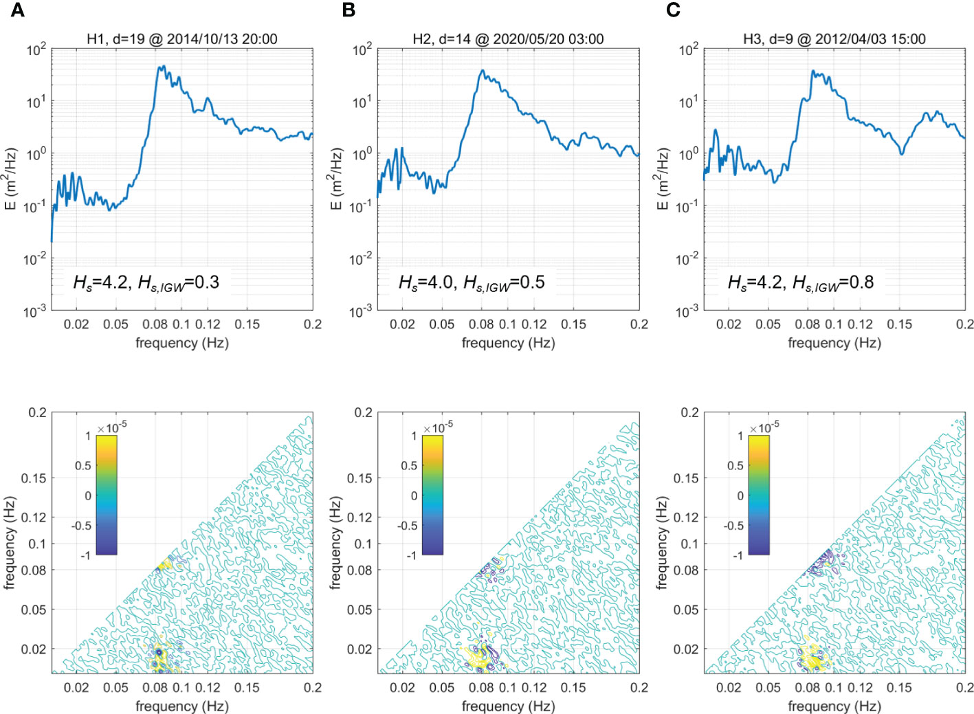
Figure 11 Imaginary parts of the bispectra (lower panels) at (A) H1, (B) H2, and (C) H3, with corresponding power spectra in the upper panels. The color bars in the lower panels show the color of the imaginary part values.The wave data were measured at different times, as each measurement time is marked in the title of the upper panels.

FIGURE 12

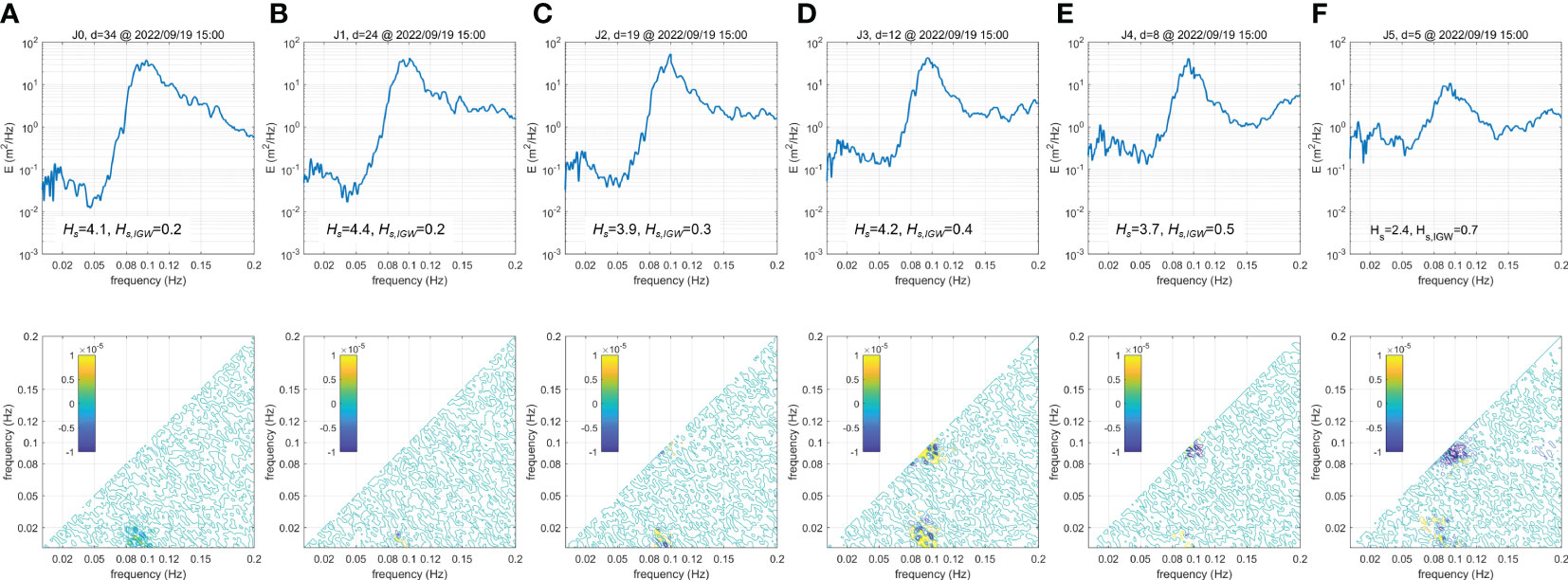
Figure 12 Imaginary parts of the bispectra (lower panels) at (A) J0, (B) J1, (C) J2, (D) J3, (E) J4, and (F) J5, with corresponding power spectra in the upper panels. The color bars in the lower panels show the color of the imaginary part values.The wave data were measured at 15:00 on 19 Sep. 2022.

In Figure 10A, the imaginary parts of the bispectra are contoured for wave station N0 at $d$=31 m. Negative values are found at $f_1$=0.08–0.10 Hz and $f_2$=0.0–0.02 Hz, where $f_1$ and $f_2$ are the frequencies on the x- and y-axis, respectively. Since the negative values at ($f_1$, $f_2$) indicate that the wave energy is transferred from $f_1$+ $f_2$ to $f_1$ and $f_2$, the results in Figure 10A show that the energy was transferred to the IGWs (0.0–0.02 Hz) from SWs (0.08–0.1 Hz) at a depth of 31 m. At $d$=14 m (N1) (Figure 10B), the transfer pattern was slightly changed. The energy was also actively transferred in the same frequency bands: $f_1$=0.08–0.10 Hz and $f_2$=0.0–0.02 Hz. However, not only negative b values but also positive values are observed, indicating that the energy was interactively transferred between the SW and IGW bands. In addition, both positive and negative values are found in the SW frequency band at $f_1$=0.08–0.10 Hz and $f_2$=0.08–0.10 Hz. Therefore, energy was transferred in the SWs between the spectral peak (0.08–0.10 Hz) and higher frequencies. The bispectral pattern at $d$=14 m becomes similar at $d$=10 m (N2), as a strong interaction between SWs and IGWs and between SW bands is also observed in Figure 10C. One difference is found at $f_1$=0.08–0.10 Hz and $f_2$=0.08–0.10 Hz, as the negative values became dominant over the positive values, indicating that the wave energy was transferred from the higher frequencies to the spectral peak at $f$=0.08–0.10 Hz. In Figure 10D, the bispectra are contoured at the shallowest depth, N3 ($d$=6 m) at Site N. The interaction between SWs and IGWs became weaker ($f_1$=0.08–0.10 Hz and $f_2$=0.0–0.02 Hz). Instead, the negative values in the SW frequency band ($f_1$=0.08–0.10 Hz and $f_2$=0.08–0.10 Hz) became prominent, which indicates that strong energy transfer occurred in the SW bands from the higher frequencies to the spectral peak.

The energy transfer pattern during wave propagation at Site N shows that wave energy transfer actively occurred between the SWs and IGWs outside the surf zone. In particular, there was evidence of energy transfer to IGWs from SWs at intermediate depths ($d$=31 m), which can support IGW shoaling. As the waves further propagated to the shore, the transfer occurred interactively between the SW and IGW frequency bands, and it stopped in the surf zone. On the other hand, energy transfer occurred within the SW bands at shallower depths ($d\le$14 m), which continued in the SW surf zone. The bispectral analysis in Figure 10, however, does not provide quantitative information on the energy transfer, so it is not possible to determine the level of transfer that contributed to the IGW shoaling.

The spatial variation pattern of the energy transfer during wave propagation at Site J is similar to that at Site N but also slightly distinct, as shown at the six wave stations in Figure 12. At J0 ($d$=33.5 m) (Figure 12A), negative values were also found in $f_1$=0.08–0.10 Hz and $f_2$=0.0–0.02 Hz, indicating that the energy was transferred to IGWs from SWs similarly to that at N0. At J1 ($d$=24 m) (Figure 12B), the negative values disappeared, showing that the energy transfer to the IGWs became weaker. The interactions between SWs and IGWs became stronger at shallower depths at J2 ($d$=19 m) and J3 ($d$=12 m) (Figures 12C, D), similar to the cases of Sites N and H. The interaction was weaker near the surf zone at J4 ($d$=8) m (Figure 12E). Note that the energy transfer between SWs and IGWs became active in the surf zone again at J5 ($d$=5 m), as shown in Figure 12F, which is distinguished from that of Site N, where the energy interaction was weak in the surf zone (Figure 10D). During wave propagation, therefore, the energy transfer actively occurred from SWs to IGWs at J0 ($d$=33.5 m), which became weak at J1 ($d$=24 m). The transfer started again from J2 ($d$=19 m) to the surf zone, and both negative and positive values were observed, indicating that energy transfer occurred interactively between SWs and IGWs. The transfer within the SW bands is also observed at shallow depths ($d\le$12 m), and the positive values disappeared with decreasing depth, indicating that the energy was transferred to the spectral peak from the higher-frequency bands. The energy transfer pattern at the three sites was similar to the results of laboratory experiments by De Bakker et al. (2015), where the energy transfer generally occurred from the spectral peak to IGW frequencies. However, the IGW–IGW interactions in the SW surf zone were not observed in this study. Instead, SW−SW interactions were observed within the surf zone.

Although the energy transfer variation during wave propagation could not be directly compared at Site H due to the inconsistency in the data measurement times, note that the energy transfer pattern at Site H is similar to those at sites N and J if the data measurement depths are also similar between the wave stations. For example, the pattern at H1 ($d$=19 m) in Figure 11A is similar to the energy transfer pattern at J2 ($d$=19 m) in Figure 12C. Similarly, the pattern at H2 ($d$=14 m) is similar to those at N1 ($d$=14 m) and J3 ($d$=12 m), and that at H3 ($d$=9 m) is similar to those at N2 ($d$=10 m) and J4 ($d$=8 m), as both positive and negative values are observed in the two corresponding frequency bands ($f_1$=0.08–0.10 Hz and $f_2$=0.0–0.02 Hz; $f_1$=0.08–0.10 Hz and $f_2$=0.08–0.10 Hz). Therefore, the results in Figure 11 indicate that the energy transfer pattern would be similar at all three sites under high wave conditions if the water depth is also similar between the wave stations, regardless of the measurement times. This finding supports the dominant IGW shoaling in this study, as it also indicates that the energy transfer between IGWs and SWs may be an important factor that contributed to shoaling.

5 Conclusions

The dependency of the IGW height on the SW parameters was investigated based on continuous (11–31 months) wave data measured at three different sites along the east coast of South Korea. At each site, wave gauges were installed in the nearshore zones from intermediate depths (30–34 m) to the surf zone (3–6 m) to observe the wave conditions during shore-approaching processes. The study examined empirical correlations between the IGW height and SW parameters for the purpose of developing a method to predict the IGW height from SW conditions for scientific and engineering applications. Two correlations that were suggested in previous studies were compared, namely, $H_{IG}$ vs. $H_s{T}_m^2$ and $H_{IG}$ vs. $H_s^2{T}_m$, as the latter is the energy flux of the SWs. The results show that linear correlations were observed at all wave stations at the three sites for both types of SW parameters. For $H_s{T}_m^2$, the IGW height showed a strong linear dependence at deeper stations, whereas the linearity became weak for the waves under the breaking regime. In contrast, SW breaking did not affect the correlation with $H_s^2{T}_m$ because the IGW height showed a strong linear dependence on the SW energy flux at shallow depths, including the breaking regime.

The IGW height correlation was also examined by estimating the proportional coefficients, $A_1$ and $A_2$, as they were the slopes of the linear lines fitted to the scatterplots between the IGW height and $H_s{T}_m^2$ and $H_s^2{T}_m$, respectively. Both $A_1$ and $A_2$ were strongly dependent on the water depth, as they increased with decreasing depth. Note that the depth dependence of the proportional coefficients showed consistent patterns, as they were fitted to logarithmic formulas (Figure 9), which could be used in developing correlations between IGW and SW parameters. When plotting the spatial variation in $A_1$ and $A_2$ in the logarithmic scales (Figures 9C, D), they were fitted to lines, and the slopes of these lines were similar between the wave stations at all three sites for both SW parameters. Regardless of the consistent pattern of the depth dependency of the proportional coefficients, a discrepancy was also observed between $A_1$ and $A_2$. The variation in $A_2$ with depth was similar between all three sites, and one formula was estimated, i.e., $A_2=-1.1\log d-2.6$. In the case of $A_1$, however, its variation was divided into two groups. The discrepancy in the $A_1$ magnitude was also observed from the power spectra in Figure 6, where the energy levels in the IGW frequency bands were higher at Site N than at Site J at wave stations with similar water depths. Although its reason is not clearly understood based on the current data sets, a similar discrepancy was also observed for seabed conditions. That is, the beaches at Site N and Site H are covered by sand, whereas the seabed at Site J is covered by rocks and gravels (Figures 1, 2). Considering that all other conditions are not distinguished between the sites based on the available data, the difference in $A_1$ values might be caused by the seabed conditions. For example, the observation in this study corresponds to that by Billson et al. (2019) in that they reported larger infragravity swash heights on sandy beaches than on gravel or mixed sand–gravel coasts.

The exponential increase in both $A_1$ and $A_2$ with decreasing depth indicates that the shoaling of IGWs was greater than that of SWs, which was also confirmed from direct comparisons of SW and IGW heights at different water depths (Figure 4). This IGW shoaling could be due to the energy transfer to the IGWs from the SWs as the imaginary part of the bispectra showed strong interactions between SW and IGW frequency bands during wave propagation. Although the bispectra analysis did not provide quantitative data on the energy transfer, the interactions between the IGWs and SWs can at least support the observation of the IGW shoaling process at the study sites. In summary, considering that the linear correlation could be applied at all water depths, including the SW breaking regime, and that the proportional coefficient, $A_2$, showed a consistent pattern between different sites, we recommend that the energy flux, $H_s^2{T}_m$, could be a preferred SW parameter for IGW height prediction at the study sites, which is also physically reasonable because shoaling could be contributed by the conservation of the energy flux when IGWs become slower with decreasing water depth (Bertin et al., 2018). However, this interpretation should be carefully considered because the $R^2$ values of $H_s^2{T}_m$ were reduced at the intermediate depths where the $R^2$ values of $H_s{T}_m^2$ were higher, indicating that $H_s{T}_m^2$ would be a better parameter for the linear regression outside the surf zone. In addition, note that the IGW energy level was different between the sites, as that of Site N was higher than that of Site J at similar water depths under similar wave conditions, which is still not understood based on the current data and requires further study.

Data availability statement

The datasets presented in this study can be found in online repositories. The names of the repository/repositories and accession number(s) can be found below: Observed Wave Height Data at 15 stations on the East Coast of South Korea [https://doi.org/10.17632/6cknvrnvh6.1].

Author contributions

J-EO, WJ, YC and KR contributed to conception and design of the study. J-EO and KR organized the database. J-EO, WJ and YC performed the statistical analysis. YC wrote the first draft of the manuscript. YC and J-EO wrote sections of the manuscript. All authors contributed to the article and approved the submitted version.

Funding

This study was supported by Korea Institute of Ocean Science and Technology (Grant/Award number: PEA0132).

Conflict of interest

The authors declare that the research was conducted in the absence of any commercial or financial relationships that could be construed as a potential conflict of interest.

Publisher’s note

All claims expressed in this article are solely those of the authors and do not necessarily represent those of their affiliated organizations, or those of the publisher, the editors and the reviewers. Any product that may be evaluated in this article, or claim that may be made by its manufacturer, is not guaranteed or endorsed by the publisher.

References

Ardhuin F., Rawat A., Aucan J. (2014). A numerical model for free infragravity waves: definition and validation at regional and global scales. Ocean Model. 77, 20–32. doi: 10.1016/j.ocemod.2014.02.006

CrossRef Full Text | Google Scholar

Baldock T. E. (2012). Dissipation of incident forced long waves in the surf zone–implications for the concept of “bound” wave release at short wave breaking. Coast. Eng. 60, 276–285. doi: 10.1016/j.coastaleng.2011.11.002

CrossRef Full Text | Google Scholar

Bellafont F. (2019). Role of infragravity waves on port agitation during storm events (Pau (FR: Université de Pau et des Pays de l'Adour).

Google Scholar

Bertin X., de Bakker A., Van Dongeren A., Coco G., André G., Ardhuin F., et al. (2018). Infragravity waves: from driving mechanisms to impacts. Earth-Science Rev. 177, 774–799. doi: 10.1016/j.earscirev.2018.01.002

CrossRef Full Text | Google Scholar

Bertin X., Martins K., de Bakker A., Chataigner T., Guérin T., Coulombier T., et al. (2020). Energy transfers and reflection of infragravity waves at a dissipative beach under storm waves. J. Geophys. Res. Oceans. 125 (5). doi: 10.1029/2019jc015714

CrossRef Full Text | Google Scholar

Billson O., Russell P., Davidson M. (2019). Storm waves at the shoreline: when and where are infragravity waves important? J. Mar. Sci. Eng. 7 (5). doi: 10.3390/jmse7050139

CrossRef Full Text | Google Scholar

Bowers E. C. (1992). Low frequency waves in intermediate depths. Proc. Int. Coast. Eng. Conf. 23rd. 832–, 845. doi: 10.1061/9780872629332.062

CrossRef Full Text | Google Scholar

Chang Y. S., Jin J. Y., Jeong W. M., Kim C. H., Do J. D. (2019). Video monitoring of shoreline positions in hujeong beach, Korea. Appl. Sci. 9 (23), 4984. doi: 10.3390/app9234984

CrossRef Full Text | Google Scholar

Cho H. Y., Jeong W. M., Oh S. H. (2014). Analysis on the characteristics of the infra-gravity waves inside and outside pohang new harbor using a transfer function model. J. Korean Soc. Coast. Ocean Eng. 26 (3), 131–139. doi: 10.9765/kscoe.2014.26.3.131

CrossRef Full Text | Google Scholar

Crawford W., Ballu V., Bertin X., Karpytchev M. (2015). The sources of deep ocean infragravity waves observed in the north Atlantic ocean. J. Geophys. Res. Oceans. 120 (7), 5120–5133. doi: 10.1002/2014jc010657

CrossRef Full Text | Google Scholar

De Bakker A. T. M., Herbers T. H. C., Smit P. B., Tissier M. F. S., Ruessink B. G. (2015). Nonlinear infragravity–wave interactions on a gently sloping laboratory beach. J. Phys. Oceanogr. 45 (2), 589–605. doi: 10.1175/jpo-d-14-0186.1

CrossRef Full Text | Google Scholar

De Bakker A. T. M., Tissier M. F. S., Ruessink B. G. (2014). Shoreline dissipation of infragravity waves. Continental. Shelf. Res. 72, 73–82. doi: 10.1016/j.csr.2013.11.013

CrossRef Full Text | Google Scholar

De Bakker A. T. M., Tissier M. F. S., Ruessink B. G. (2016). Beach steepness effects on nonlinear infragravity-wave interactions: a numerical study. J. Geophys. Res. Oceans. 121 (1), 554–570. doi: 10.1002/2015jc011268

CrossRef Full Text | Google Scholar

Do J. D., Jin J. Y., Jeong W. M., Lee B., Choi J. Y., Chang Y. S. (2021). Collapse of a coastal revetment due to the combined effect of anthropogenic and natural disturbances. Sustainability. 13 (7). doi: 10.3390/su13073712

CrossRef Full Text | Google Scholar

Elgar S., Guza R. T. (1985). Observations of bispectra of shoaling surface gravity waves. J. Fluid Mech. 161, 425–448. doi: 10.1017/S0022112085003007

CrossRef Full Text | Google Scholar

Elgar S., Herbers T. H. C., Okihiro M., Oltman-Shay J., Guza R. T. (1992). Observations of infragravity waves. J. Geophys. Res. Oceans 97 (C10), 15573–15577. doi: 10.1029/92jc01316

CrossRef Full Text | Google Scholar

Fiedler J. W., Brodie K. L., McNinch J. E., Guza R. T. (2015). Observations of runup and energy flux on a low-slope beach with high-energy, long-period ocean swell. Geophys. Res. Lett. 42 (22), 9933–9941. doi: 10.1002/2015gl066124

CrossRef Full Text | Google Scholar

Gao J., Ma X., Zang J., Dong G., Ma X., Zhu Y., et al. (2020). Numerical investigation of harbor oscillations induced by focused transient wave groups. Coast. Eng. 158, 103670. doi: 10.1016/j.coastaleng.2020.103670

CrossRef Full Text | Google Scholar

Gao J., Zhou X., Zhou L., Zang J., Chen H. (2019). Numerical investigation on effects of fringing reefs on low-frequency oscillations within a harbor. Ocean Eng. 172, 86–95. doi: 10.1016/j.oceaneng.2018.11.048

CrossRef Full Text | Google Scholar

Guza R. T., Thornton E. B. (1982). Swash oscillations on a natural beach. J. Geophys. Res. Oceans. 87 (C1), 483–491. doi: 10.1029/JC087iC01p00483

CrossRef Full Text | Google Scholar

Guza R. T., Thornton E. B. (1985). Observations of surf beat. J. Geophys. Res. Oceans. 90 (C2), 3161–3172. doi: 10.1029/JC090iC02p03161

CrossRef Full Text | Google Scholar

Hasselmann K., Munk W., MacDonald G. J. F. (1963). “Bispectra of ocean waves,” in Symposium on time series analysis. Ed. Rosenblatt M. (NY: John Wiley), 125–139.

Google Scholar

Henderson S. M., Guza R. T., Elgar S., Herbers T. H. C., Bowen A. J. (2006). Nonlinear generation and loss of infragravity wave energy. J. Geophys. Res. Oceans 111 (C12). doi: 10.1029/2006jc003539

CrossRef Full Text | Google Scholar

Herbers T. H. C., Elgar S., Guza R. T. (1995a). Generation and propagation of infragravity waves. J. Geophys. Res. Oceans. 100 (C12), 24863–24872. doi: 10.1029/95JC02680

CrossRef Full Text | Google Scholar

Herbers T. H. C., Elgar S., Guza R. T., O'Reilly W. C. (1995b). Infragravity-frequency (0.005–0.05 Hz) motions on the shelf. part II: free waves. J. Phys. Oceanogr. 25 (6), 1063–1079. doi: 10.1175/1520-0485(1995)025<1063:IFHMOT>2.0.CO;2

CrossRef Full Text | Google Scholar

Herbers T., Russnogle N., Elgar S. (2000). Spectral energy balance of breaking waves within the surf zone. J. Phys. Oceanogr. 30, 2723–2737. doi: 10.1175/1520-0485(2000)030<2723:SEBOBW>2.0.CO;2

CrossRef Full Text | Google Scholar

Holman R. A. (1981). Infragravity energy in the surf zone. J. Geophys. Res. Oceans. 86 (C7), 6442–6450. doi: 10.1029/JC086iC07p06442

CrossRef Full Text | Google Scholar

Holthuijsen L. H. (2007). Waves in oceanic and coastal waters (NY: Cambridge Univ. Press).

Google Scholar

Huntley D. A., Davidson M., Russell P., Foote Y., Hardisty J. (1993). Long waves and sediment movement on beaches: recent observations and implications for modelling. J. Coast. Res., 215–229.

Google Scholar

Inch K., Davidson M., Masselink G., Russell P. (2017). Observations of nearshore infragravity wave dynamics under high energy swell and wind-wave conditions. Cont. Shelf Res. 138, 19–31. doi: 10.1016/j.csr.2017.02.010

CrossRef Full Text | Google Scholar

Jeong W. M., Park W. S., Kim K. H., Kim J. H. (2002). Correlations between long-and short-period waves in shallow water region around sokcho harbor. KSCE J. Civ. Eng. 22 (5B), 711–721.

Google Scholar

Li S., Liao Z., Liu Y., Zou Q. (2020). Evolution of infragravity waves over a shoal under nonbreaking conditions. J. Geophys. Res. Oceans. 125 (8). doi: 10.1029/2019jc015864

CrossRef Full Text | Google Scholar

Longuet-Higgins M. S. (1962). Resonant interactions between two trains of gravity waves. J. Fluid Mech. 12 (3), 321–332. doi: 10.1017/S0022112062000233

CrossRef Full Text | Google Scholar

Mahmoudof S. M., Azizpour J., Eyhavand-Koohzadi A. (2021). Observation of infragravity wave processes near the coastal cliffs of chabahar (Gulf of Oman). Estuar. Coast. Shelf Sci. 251, 107226. doi: 10.1016/j.ecss.2021.107226

CrossRef Full Text | Google Scholar

McComb P., Gorman R., Goring D. (2005). “Forecasting infragravity wave energy within a harbour,” in Proc. Waves 2005 Conf. 3–7(Madrid).

Google Scholar

Munk W. H. (1949). The solitary wave theory and its application to surf problems. Ann. N. Y. Acad. Sci. 51 (3), 376–424. doi: 10.1111/j.1749-6632.1949.tb27281.x

CrossRef Full Text | Google Scholar

Nelson R. C., Treloar P. D., Lawson N. V. (1988). The dependency of inshore long waves on the characteristics of offshore short waves. Coast. Eng. 12 (3), 213–231. doi: 10.1016/0378-3839(88)90006-3

CrossRef Full Text | Google Scholar

Oh J. E., Jeong W. M. (2023). Observed wave height data at 15 stations on the East coast of south Korea, mendeley data, V1. doi: 10.17632/6cknvrnvh6.1

CrossRef Full Text | Google Scholar

Oh J. E., Jeong W. M., Chang Y. S., Oh S. H. (2020). On the separation period discriminating gravity and infragravity waves off gyeongpo beach, Korea. J. Mar. Sci. Eng. 8 (3). doi: 10.3390/jmse8030167

CrossRef Full Text | Google Scholar

Poate T., Masselink G., Austin M. J., Inch K., Dickson M., McCall R. (2020). Infragravity wave generation on shore platforms: bound long wave versus breakpoint forcing. Geomorphology. 350. doi: 10.1016/j.geomorph.2019.106880

CrossRef Full Text | Google Scholar

Pomeroy A., Lowe R., Symonds G., Van Dongeren A., Moore C. (2012). The dynamics of infragravity wave transformation over a fringing reef. J. Geophys. Res. Oceans. 117 (C11). doi: 10.1029/2012jc008310

CrossRef Full Text | Google Scholar

Rawat A., Ardhuin F., Ballu V., Crawford W., Corela C., Aucan J. (2014). Infragravity waves across the oceans. Geophys. Res. Lett. 41 (22), 7957–7963. doi: 10.1002/2014gl061604

CrossRef Full Text | Google Scholar

Roelvink D., Reniers A., Van Dongeren A. P., De Vries J. V. T., McCall R., Lescinski J. (2009). Modelling storm impacts on beaches, dunes and barrier islands. Coast. Eng. 56 (11-12), 1133–1152. doi: 10.1016/j.coastaleng.2009.08.006

CrossRef Full Text | Google Scholar

Ruessink B. G. (1998). Bound and free infragravity waves in the nearshore zone under breaking and nonbreaking conditions. J. Geophys. Res. Oceans 103 (C6), 12795–12805.

Google Scholar

Ruessink B. G. (2010). Observations of turbulence within a natural surf zone. J. Phys. Oceanogr. 40 (12), 2696–2712. doi: 10.1175/2010jpo4466.1

CrossRef Full Text | Google Scholar

Sheremet A. (2002). Observations of nearshore infragravity waves: seaward and shoreward propagating components. J. Geophys. Res. Oceans. 107 (C8). doi: 10.1029/2001jc000970

CrossRef Full Text | Google Scholar

Smit P. B., Janssen T. T., Herbers T. H. C., Taira T., Romanowicz B. A. (2018). Infragravity wave radiation across the shelf break. J. Geophys. Res. Oceans. 123 (7), 4483–4490. doi: 10.1029/2018jc013986

CrossRef Full Text | Google Scholar

Symonds G., Huntley D. A., Bowen A. J. (1982). Two-dimensional surf beat: long wave generation by a time-varying breakpoint. J. Geophys. Res. Oceans. 87 (C1), 492–498. doi: 10.1029/JC087iC01p00492

CrossRef Full Text | Google Scholar

Tolman H. L. (2008). A mosaic approach to wind wave modeling. Ocean Model. 25 (1-2), 35–47. doi: 10.1016/j.ocemod.2008.06.005

CrossRef Full Text | Google Scholar

Tucker M. (1950). Surf beats: Sea waves of 1 to 5 min. period. Proc. Math. Phys. Eng. Sci. 202 (1071), 565–573. doi: 10.1098/rspa.1950.0120

CrossRef Full Text | Google Scholar

Van Dongeren A. R. J. A., Battjes J., Janssen T., Van Noorloos J., Steenhauer K., Steenbergen G., et al. (2007). Shoaling and shoreline dissipation of low-frequency waves. J. Geophys. Res. Oceans. 112 (C2). doi: 10.1029/2006jc003701

CrossRef Full Text | Google Scholar

Van Dongeren A. P., Lowe R., Pomeroy A., Trang D. M., Roelvink D., Symonds G., et al. (2013). Numerical modeling of low-frequency wave dynamics over a fringing coral reef. Coast. Eng. 73, 178–190. doi: 10.1016/j.coastaleng.2012.11.004

CrossRef Full Text | Google Scholar

Vasan V., Oliveras K., Henderson D., Deconinck B. (2017). A method to recover water-wave profiles from pressure measurements. Wave Motion. 75, 25–35. doi: 10.1016/j.wavemoti.2017.08.003

CrossRef Full Text | Google Scholar

Zhang Q., Toorman E. A., Monbaliu J. (2020). Shoaling of bound infragravity waves on plane slopes for bichromatic wave conditions. Coast. Eng. 158. doi: 10.1016/j.coastaleng.2020.103684

CrossRef Full Text | Google Scholar