Deformation analysis of underwater shield tunnelling based on HSS model parameter obtained by the Bayesian approach

1 Introduction

In recent years, many underwater tunnels have been built worldwide because of their various advantages, such as all-weather operation and not affecting navigation (Huang and Zhan, 2019; Qiu et al., 2019; Tang et al., 2021). By the end of 2020, 245 underwater tunnels have been built in China, mainly in the Huangpu River, the Pearl River and the Yangtze River. There are three main methods of tunnel construction, including drill-and-blast, shield tunnelling and immersed tube methods, among which shield tunnelling is the most widely used one (Lin et al., 2013). With the increasing scale of underwater tunnels, shield diameter and tunnelling distance are constantly refreshed. The most representative underwater large-diameter shield tunnel projects in China include Wuhan Heping Avenue South Extension, Jinan Yellow River Tunnel and Nanjing Yangtze River Tunnel, whose excavation diameters are more than 14 m. Although a wealth of experience has been accumulated in the construction of underwater large-diameter shield tunnels, the disturbance of the surrounding soil caused by shield tunnelling is still unavoidable. Therefore, the core problem of underwater large-diameter shield tunnel construction is how to control the stability of shield tunnelling to minimize the construction deformation, especially under high water pressure and shallow overburden conditions.

Numerical simulation techniques have become a crucial tool for analyzing challenging geotechnical engineering problems due to significant advancements in computer technology. However, the reliability of numerical simulation results mainly depends on the selection of geotechnical constitutive model and its parameters. Many studies (Jardine et al., 1986; Burland, 1989) have already shown that soil strain in most areas around underground structures such as tunnels was within the range of 0.01% - 0.1%, which belongs to the small strains. Meanwhile, numerical simulation studies have shown that the soil deformation and stress distribution of underground structures predicted by the commonly used Mohr-Coulomb model is different from the actual ones and sometimes even greatly overestimated. On the other hand, the model considering the nonlinear small strain stiffness of soil can accurately represent the associated deformation laws (Zhang et al., 2019; Zhou et al., 2020). The hardening soil model with small strain stiffness (HSS) model is widely used to assess the response and control of underground construction under small strain conditions in soils (Likitlersuang et al., 2013; Ng et al., 2020). HSS model contains 13 parameters which are difficult to determine each parameter in the tunnel project through laboratory tests due to the lengthy acquisition cycle. To simplify the application of HSS model, many researchers have summarized the empirical correlations between reference secant modulus $E_{50}^{\text{ref}}$, reference tangent modulus $E_{\text{oed}}^{\text{ref}}$ and reference unloading/reloading modulus $E_{\text{ur}}^{\text{ref}}$ through laboratory tests and back analysis (Wang et al., 2012; Huang et al., 2013; Ng et al., 2020). Although there are different empirical correlations between different regions and soils, it is appropriate to set $E_{\text{ur}}^{\text{ref}}$ = 3 $E_{50}^{\text{ref}}$= 3 $E_{\text{oed}}^{\text{ref}}$ in many practical cases. $E_{50}^{\text{ref}}$ denotes the reference secant modulus corresponding to 50% of the failure load of the triaxial consolidation drainage test when the reference stress p^ref is 100 kPa, reflecting the shear hardening characteristics of soil. It can be seen that $E_{50}^{\text{ref}}$ can be used as a critical parameter to obtain other stiffness parameters.

In-situ testing is preferable for underwater tunnel projects where soil sampling is challenging in submerged locations. Piezocone penetration test (CPTU) is one of the most widely used methods, with the advantages of high repeatability, accuracy and the ability to obtain continuous stratigraphic profiles with different strata in vertical directions (Cai et al., 2017; Mo et al., 2020). These advantages facilitate the fast acquisition of HSS model parameters. However, the geotechnical parameters required for engineering can not be directly given by CPTU, extensive research must be conducted to develop transformation models of CPTU data with geotechnical parameters (Sadrekarimi, 2016). To date, there are still few studies on HSS model parameters obtained by converting CPTU test data. Further work needs to be carried out to establish the connection between the two and obtain geotechnical parameters. And the transformation accuracy also needs to be improved.

In recent years, the Bayesian approach has provided a new way to solve the problem of probabilistic characterization of soil parameters in geotechnical engineering, such as Young’s modulus (E_u) (Wang and Cao, 2013), effective friction angle (φ^’) (Tian et al., 2016), soil behaviour type index I_c (Cao et al., 2019), coefficient of consolidation in the horizontal direction (c_h) (Zhao et al., 2022). Under a Bayesian framework, the engineering experience is quantified as prior knowledge and can subsequently be updated by the likelihood function integrated with test information. Finally, posterior knowledge considering various uncertainties can be obtained (Cao et al., 2016; Wang et al., 2016; Ching and Phoon, 2019). However, the application of the Bayesian approach in probabilistic characterization of $E_{50}^{\text{ref}}$ has not been reported.

This paper focuses on the approach of obtaining geotechnical parameters of underwater large-diameter shield tunnel and its construction deformation mechanism and response. The transformation model between the CPTU test data and the reference secant modulus $E_{50}^{\text{ref}}$ and effective internal friction angle φ^’ of the HSS model in the Jinan Yellow River basin silty clay was constructed. A Bayesian probability characterization approach for the HSS model with $E_{50}^{\text{ref}}$ of silty clay based on CPTU was proposed, which obtained the most probable values of $E_{50}^{\text{ref}}$. The obtained model parameters were applied to the Yellow River tunnel project to analyze the deformation laws of underwater large-diameter shield construction.

2 Study area

The Jinan Yellow River Tunnel project is located in Tianqiao District, connecting Queshan north and Jiluo road south. With a section length of 2519 m, this tunnel goes underneath the Yellow River. The tunnel adopts a highway and rail transit joint construction scheme with roads arranged on the upper layer and M2 metro sections arranged on the lower layer. The diameter of slurry shield machine is 15.76 m, and the external and internal radius of the lining is 15.2 m and 13.9 m, respectively. The lining ring consists of 10 segments with a width of 2.0 m and a thickness of 0.6 m. According to the site investigation, the site mainly goes through silt clay containing local calcareous nodules and fine sand, underlying soil is completely weathered gabbro. The tunnel buried depth is 11.2 - 42.3 m, and the maximum water pressure is 0.65 MPa. Figure 1 shows the project overview and a typical geological profile.

FIGURE 1

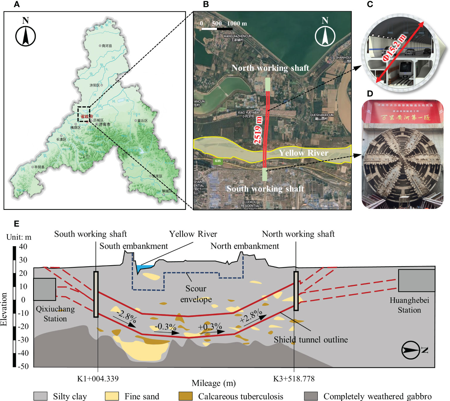
Figure 1 Project overview: (A, B) Location of the Jinan Yellow River Tunnel project. (C) Tunnel structure. (D) Shield cutter head. (E) Longitudinal section of engineering geology.

3 Methodology

3.1 Transformation model

3.1.1 Cavity expansion model

Following the work of Randolph et al. (1994), the cone tip resistance q_c is related to the limit pressure p_lim during the spherical cavity expansion. When using a more practical complex constitutive model, numerical analysis is often required for simplified calculations. A spherical cavity expansion was modelled in the Plaxis 2D to simulate the penetration process, following similar procedures described by Xu and Lehane (2008) and Suryasentana and Lehane (2014). Considering the symmetry of spherical cavity expansion, the model dimension is x = 12 m, y = 24 m. According to the studies of Suzuki (2015) and Xu (2007), there are no boundary effects. The initial radius of the spherical cavity a₀ is 0.1 m. A positive volume strain of 10% is applied to the cavity cluster in multiple stages to simulate the gradual expansion. The construction phase of the model is divided into 21 steps. Before calculation, 7 nodes and 8 stress points around the cavity wall are selected as output. Finally, the selected nodes and stress points data are averaged separately to plot the relationship between the limit pressure p_lim and excess pore pressure Δu with the normalized displacement a/a₀. The cone tip resistance q_c is obtained from the following relationship: $q_{\text{c}}=p_{\text{lim}}+\sqrt{3}[c^{\prime }+(p_{\text{lim}}-u)]\text{tan}{\phi }^{\prime }$.

3.1.2 Correlations between q_c and $E_{50}^{\text{ref}}$

In order to correct the relationship proposed by Suzuki (2015), Table 1 listed 15 analysis cases to study the influence of model parameters $E_{50}^{\text{ref}}$ and φ^’ on the limit pressure p_lim using the HSS model. The influence of the over consolidation ratio is not considered (OCR = 1). The permeability coefficient of soil is 0.02 m/d (2.3×10^-7 m/s), according to the geological prospecting report.

TABLE 1

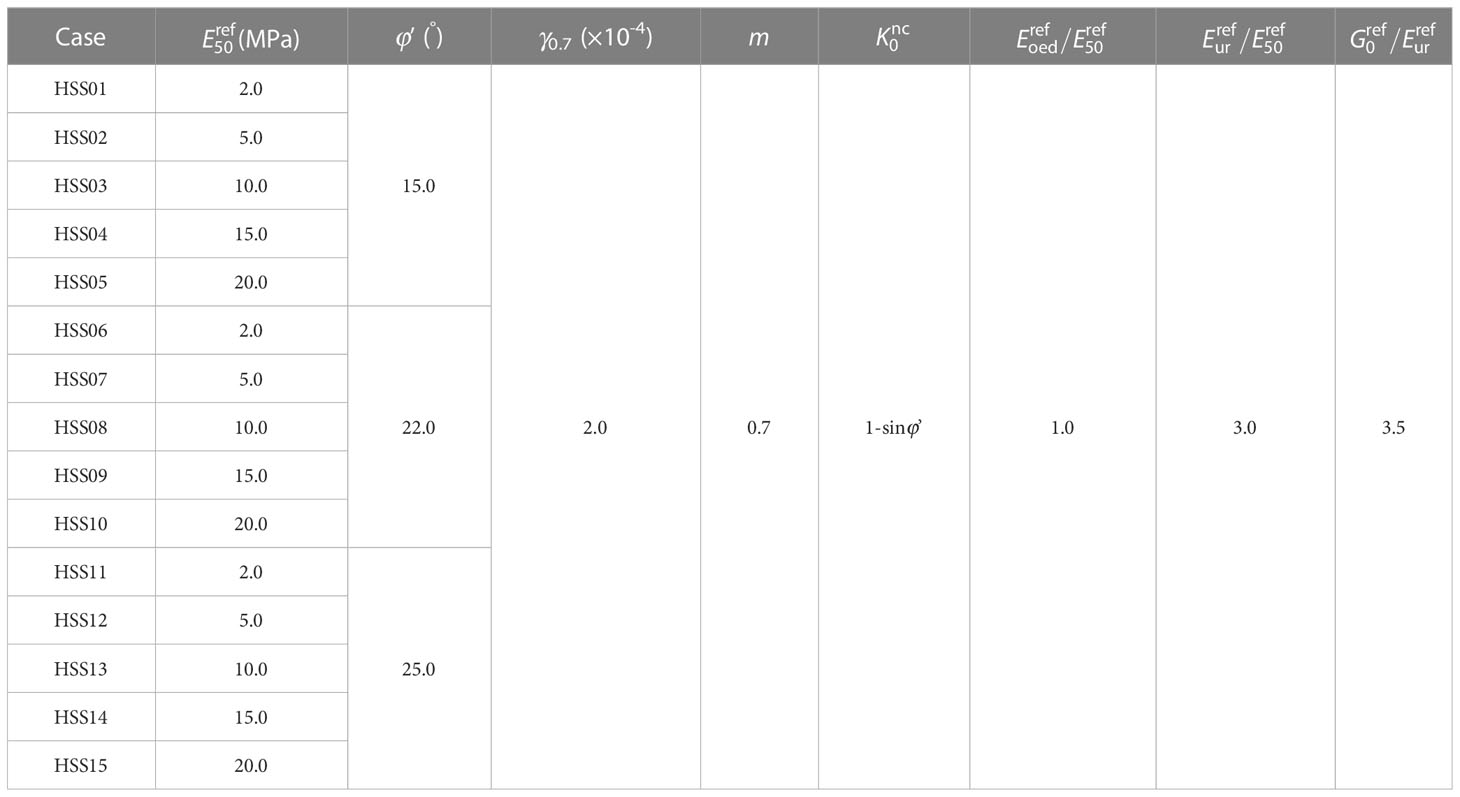
Table 1 Research scheme of spherical cavity expansion based on the HSS model.

The cone tip resistance q_c can be obtained by substituting the limit pressure p_lim of each group into the formula. Therefore, the normalized cone tip resistance Q, $E_{50}^{\text{ref}}$/p’₀ and φ^’ are drawn in Figure 2. The relationship between logQ and log($E_{50}^{\text{ref}}$/p’₀) is almost linear in logarithmic coordinates. According to the results proposed by Suzuki (2015) based on the HS model, the normalized cone tip resistance Q relation based on the HSS model can be obtained as follows:

FIGURE 2

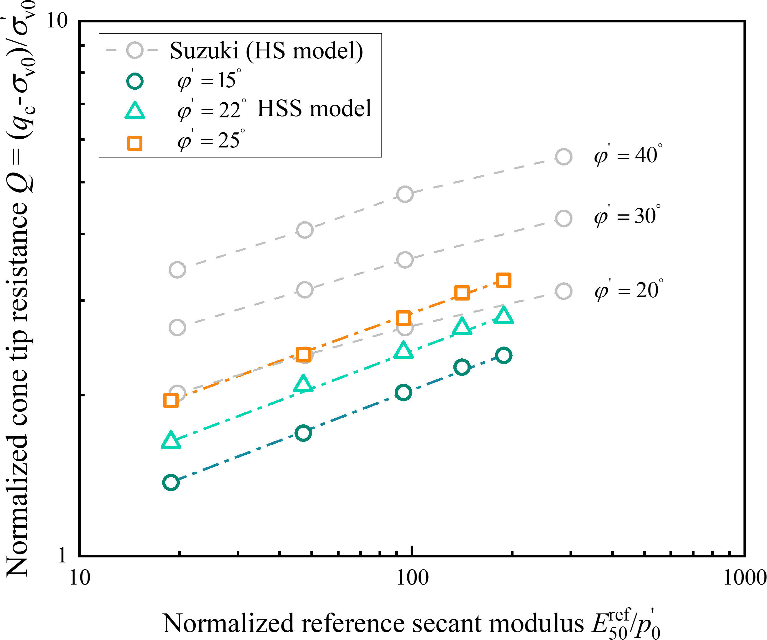
Figure 2 Relationship between normalized cone tip resistance Q and reference secant modulus $E_{50}^{\text{ref}}$ and effective internal friction angle φ^’.

$\begin{array}{ll}Q=\frac{q_{\text{c}}-{\sigma }_{\text{v}0}}{{\sigma }_{\text{v}0}^{\text{'}}}=1.4{(\frac{E_{50}^{ref}}{p_0^{\text{'}}})}^{0.23}{(\text{sin}{\phi }^{\prime })}^{0.47}& (1)\end{array}$

3.2 Calibration chamber test

To verify the applicability of the relationship for Jinan silty clay, a mini CPTU calibration chamber test of remolded soil was conducted. Figure 3 shows the calibration chamber system, including the calibration chamber, loading device, pump and mini CPTU. The chamber contains test soil with a height of 600 mm and a diameter of 525 mm. The chamber wall is 40 mm thick to maintain K₀ consolidation. To ensure that the soil sample height can meet the penetration requirements after consolidation, a 300 mm high ring with the same diameter is added to the upper part of the chamber to accommodate the slurry during consolidation. Vertical stresses can be independently controlled by the pump, providing a maximum vertical load of 200 kPa. The loading plate is equipped with four penetration holes and one spare hole. The diameter of the hole is 16 mm, and the distance between the penetration holes is 10 times the mini CPTU diameter, which can effectively reduce the influence of boundary effects on the test data. The mini CPTU used in the calibration chamber tests has a diameter of 16 mm and a cone angle of 60^°. Due to the instability of the sleeve friction test results, the CPTU is not equipped with a sleeve friction sensor, but only with the cone tip resistance and pore pressure sensor. A servo motor controls the CPTU to penetrate the soil from the reserved hole at a constant rate of 20 mm/s.

FIGURE 3

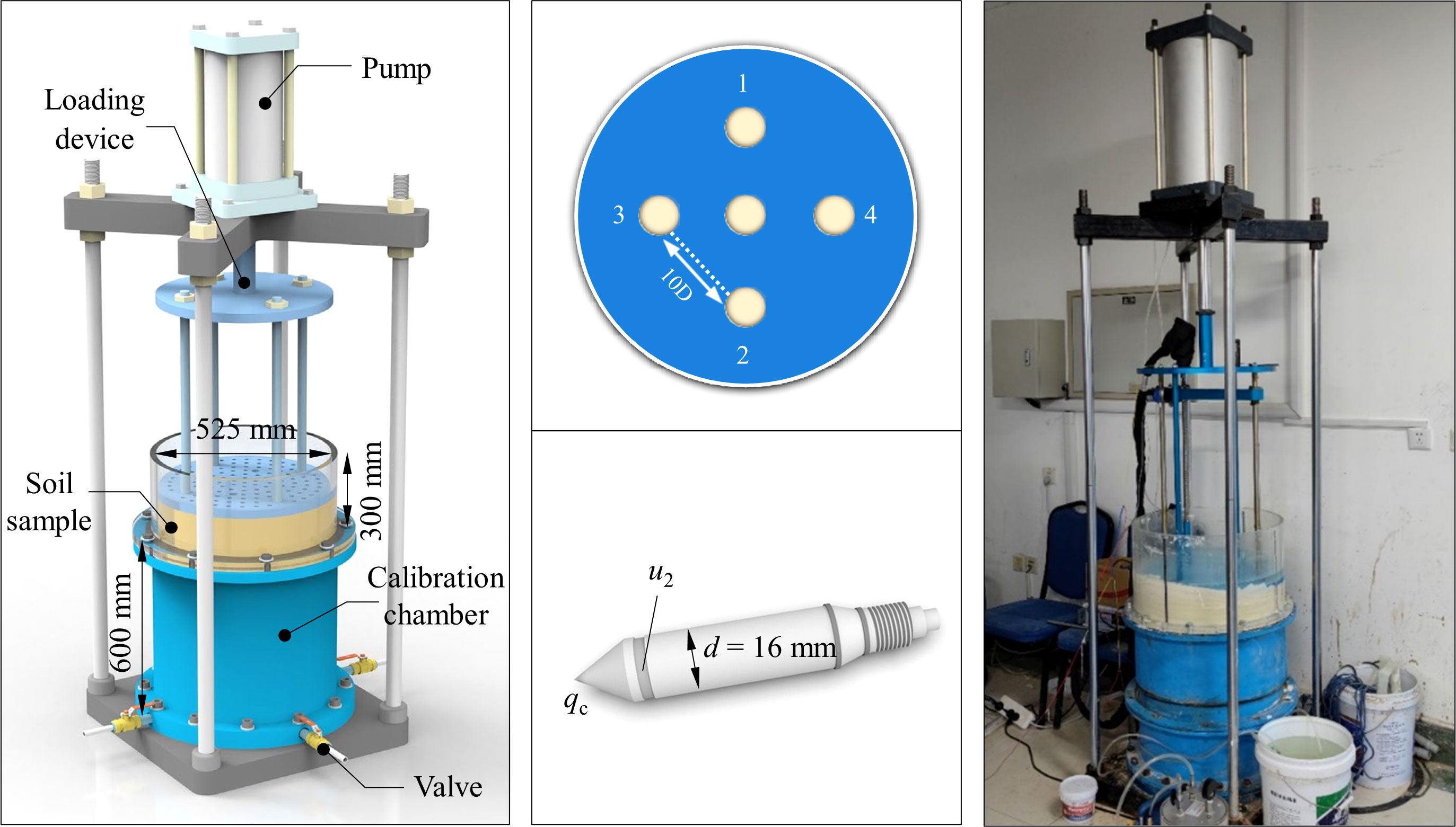
Figure 3 Calibration chamber system.

Remolded specimens of silt clay, taken from about 10 m deep in the north working shaft of the Yellow River Tunnel project, were prepared and tested. The primary property index of soils was obtained by laboratory tests. The water content is 23.0%. Liquid limit and plastic limit are 33.5% and 19.0%, respectively. The initial void ratio is 0.67.

For the calibration chamber test, cylindrical soil samples were prepared using the slurry consolidation method. Then, apply the overburden stress of 100 kPa and measure the vertical deformation twice a day. When the deformation is less than 0.1mm/d, the test can be started. The consolidation time of this experiment is 16 d. After consolidation, the penetration test procedure is as follows: Remove the geotextiles from the surface of the soil sample and connect the saturated mini CPTU with the penetration equipment. Keep the CPTU probe below the chamber’s water level before the test begins. Then, click the computer with the data acquisition instrument and start the penetration test. The test was stopped when the CPTU penetration depth reached 300 mm. After the completion of the first test, the geotextile was readjusted and the pressure was reset to 100 kPa. The next set of penetration tests was conducted after consolidation for 1 h. Repeat the above steps for four tests.

Figure 4 shows the results of four repeated tests in saturated remolded specimens. The penetration was performed to a depth of about 300 mm, at which stage the distance to the bottom boundary was about 200 mm (about 12 times the cone diameter). From the results of cone tip resistance q_c, it can be seen that q_c increases rapidly when the CPTU starts to penetrate the shallow surface soil (about 50 mm). The maximum values of the four repeated tests differed greatly, with the maximum reaching about 500 kPa and the minimum about 350 kPa. This phenomenon is mainly caused by surface soil over consolidation. When the CPTU penetration reaches 50 - 150 mm, the q_c fluctuation range decreases significantly. It enters the stable penetration zone until the penetration depth exceeds 150 mm. The cone tip resistance q_c of the four groups of tests is 331.6 kPa, 313.4 kPa, 338.6 kPa, and 324.4 kPa, respectively. Similar to the cone tip resistance, when the CPTU penetrated 150 mm, the gap between the results of the excess pore pressure Δu gradually decreased. The excess pore pressure Δu is 150.3 kPa, 151.2 kPa, 143.2 kPa and 155.7 kPa, respectively.

FIGURE 4

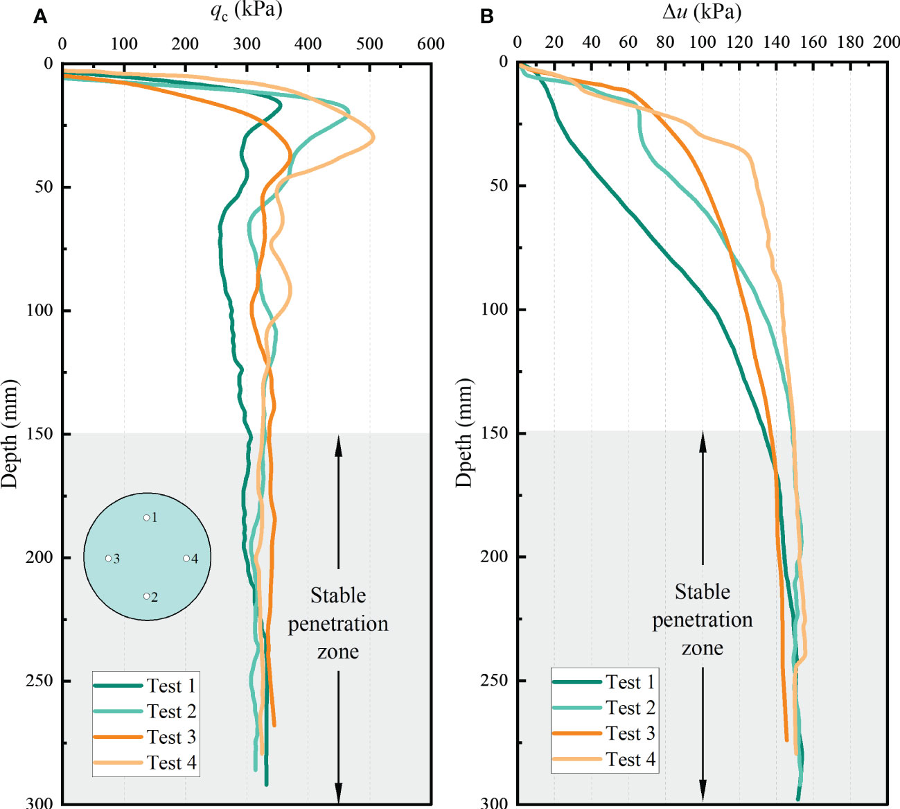
Figure 4 Calibration chamber test results: (A) Relationship between cone tip resistance q_c and depth h (B) Relationship between excess pore pressure Δu and depth h.

3.3 Transformation model verification

To verify the applicability of formula (1) in silty clay, the results of cone tip resistance q_c of the CPTU calibration chamber test were substituted into formula (1), and the calculated $E_{50}^{\text{ref}}$ was finally obtained, as shown in Figure 5. With the increase of q_c, the $E_{50}^{\text{ref}}$ also increases, which is basically linear. At the same time, the $E_{50}^{\text{ref}}$ test values of the undisturbed soil and the remolded soil obtained through the triaxial consolidation drainage test are also shown in Figure 5, respectively 6.4 MPa and 5.3 MPa. It can be seen that all the calculated values are located near the test values, and the calculated mean value is 6.1MPa, which is relatively close to the test value of undisturbed soil, with a deviation of 4.9%. The deviation from $E_{50}^{\text{ref}}$ test value of remolded soil is 13.1%. Thus, $E_{50}^{\text{ref}}$ calculated by the formula (1) is reliable and suitable for CPTU penetration in silty clay.

FIGURE 5

Figure 5 Comparison between calculated values and experimental values of $E_{50}^{\text{ref}}$.

3.4 Bayesian probability characterization of $E_{50}^{\text{ref}}$

3.4.1 Inherent variability of $E_{50}^{\text{ref}}$

The influence factors such as particle composition and transport process lead to different soil properties. Therefore, there is inherent variability in soil, independent of the knowledge state of geotechnical properties, and will not decrease with the increase of knowledge (Phoon and Kulhawy, 1999; Wang and Cao, 2013; Wang et al., 2023). $E_{50}^{\text{ref}}$ is a continuous variable and must be non-negative because of its physical meaning. Therefore, geotechnical parameters are often modeled as logarithmic normal random variables (Wang and Cao, 2013). Assume that $E_{50}^{\text{ref}}$ is a lognormal random variable with a mean μ and a standard deviation σ, expressed as

$\begin{array}{ll}\ln E_{50}^{\text{ref}}={\mu }_N+{\sigma }_{N}z& (2)\end{array}$

in which μ_N and σ_N are the mean and standard deviation of ln $E_{50}^{\text{ref}}$, z is a normal random variable with a mean of 0 and SD of 1.

3.4.2 Transformation uncertainty

Eq. (1) can be rewritten in a log-log scale as:

$\begin{array}{ll}\text{lnQ}=a\ln E_{50}^{\text{ref}}+\text{b}+ϵ& (3)\end{array}$

in which lnQ is normalized cone tip resistance in a log scale; a, b is the coefficient, ϵ is a Gaussian variable representing the transformation uncertainty.

Combining Eqs. (2) and (3) lead to:

$\begin{array}{ll}\text{lnQ}=(a{\mu }_N+\text{b})+a{\sigma }_N\text{z}+ϵ& (4)\end{array}$

3.4.3 Bayesian framework

For the given prior knowledge and CPTU data, the probability density function of $E_{50}^{\text{ref}}$ can be expressed as:

$\begin{array}{ll}P(E_{50}^{\text{ref}}\mid \text{Data},\text{Prior})={{\displaystyle \int }}_{\mu ,\sigma }P(E_{50}^{\text{ref}}\mid \mu ,\sigma )P(\mu ,\sigma \mid \text{Data},\text{Prior})\text{d}\mu \text{d}\sigma & (5)\end{array}$

in which P($E_{50}^{\text{ref}}$|μ,σ) is the conditional probability of a given set of μ and σ. Because $E_{50}^{\text{ref}}$ is lognormally distributed, it can be expressed as:

$\begin{array}{ll}P(E_{50}^{\text{ref}}\mid \mu ,\sigma )=\frac{1}{\sqrt{2\text{π}}{\sigma }_N{E}_{50}^{\text{ref}}}\text{exp}\left\{-\frac{1}{2}{[\frac{\text{l}n{E}_{50}^{\text{ref}}-{\mu }_N}{{\sigma }_N}]}^2\right\}& (6)\end{array}$

Using Bayesian formula, P(μ,σ|Data, Prior) can be expressed as:

$\begin{array}{ll}P(\mu ,\sigma \text{∣Data},\text{Prior})=(\mu ,\sigma \text{∣Data})=KP(\text{Data}\mid \mu ,\sigma )P(\mu ,\sigma )& (7)\end{array}$

in which K is a normalized constant independent of μ and σ; Data = {lnQ_i, i=1, 2, …, n_s} is a set of CPTU test data; P(Data|μ,σ) is the likelihood function which is expressed as:

$\begin{array}{ll}P(\text{Data∣}\mu ,\sigma )={\displaystyle \prod _{i=1}^n\frac{1}{\sqrt{2\text{π}}\sqrt{{(a{\sigma }_N)}^2+{\sigma }_{ϵ}^2}}}exp\left\{-\frac{1}{2}{[\frac{\text{ln}{Q}_i-(a{\sigma }_N+\text{b})}{\sqrt{{(a{\sigma }_N)}^2+{\sigma }_{ϵ}^2}}]}^2\right\}& (8)\end{array}$

P(μ,σ) is assumed to be a uniform distribution, expressed as:

$\begin{array}{ll}P(\mu ,\sigma )=\frac{1}{{\mu }_{\text{max}}-{\mu }_{\text{min}}}\times \frac{1}{{\sigma }_{\text{max}}-{\sigma }_{\text{min}}},\mu \in [{\mu }_{\text{min}}, {\mu }_{\text{max}}],\sigma \in [{\sigma }_{\text{min}},{\sigma }_{\text{max}}]& (9)\end{array}$

Substitute Eqs. (6) - (9) into Eqs. (5) to obtain the posterior probability density function of $E_{50}^{\text{ref}}$ calculated according to the approach proposed by Wang and Cao (2013).

4 Results and discussion

4.1 Probability distribution of $E_{50}^{\text{ref}}$

Consider a set of prior knowledge, μ∈[3.9, 8.0], σ∈[0.5, 3.0]. And using CPTU field test data from the Jinan Yellow River Basin as input data for Bayesian inversion, the scatter diagram of $E_{50}^{\text{ref}}$ is shown in Figure 6A. Most samples are between 3.0 and 10.0 MPa. With the increase of the sample value, the scatter gradually becomes sparse, and all the sample values are less than 25 MPa. Further analysis from the statistical histogram (Figure 6B) shows 27367 sample points in 3.0 - 10.0 MPa, accounting for 91.0%. It peaks in the 6.0 - 7.0 MPa interval with a sample size of 6481. Figure 6C is the probability density function of $E_{50}^{\text{ref}}$ estimated by Figure 6A, and it also includes the value of $E_{50}^{\text{ref}}$ obtained from $E_{50}^{\text{ref}}$= E_s1-2. E_s1-2 is the compression modulus of undisturbed soil. 93.8% of the undisturbed soil data is within the range of 3.0 - 10.0 MPa, which is consistent with the inversion results. Figure 6D plots the cumulative distribution function of $E_{50}^{\text{ref}}$. The cumulative distribution function of equivalent samples and that obtained from empirical correlation have a good consistency. Such a good agreement demonstrates that the information in the equivalent samples is consistent with the information obtained through empirical correlation. Also, the approach used to estimate the distribution of $E_{50}^{\text{ref}}$ is feasible in Jinan silty clay.

FIGURE 6

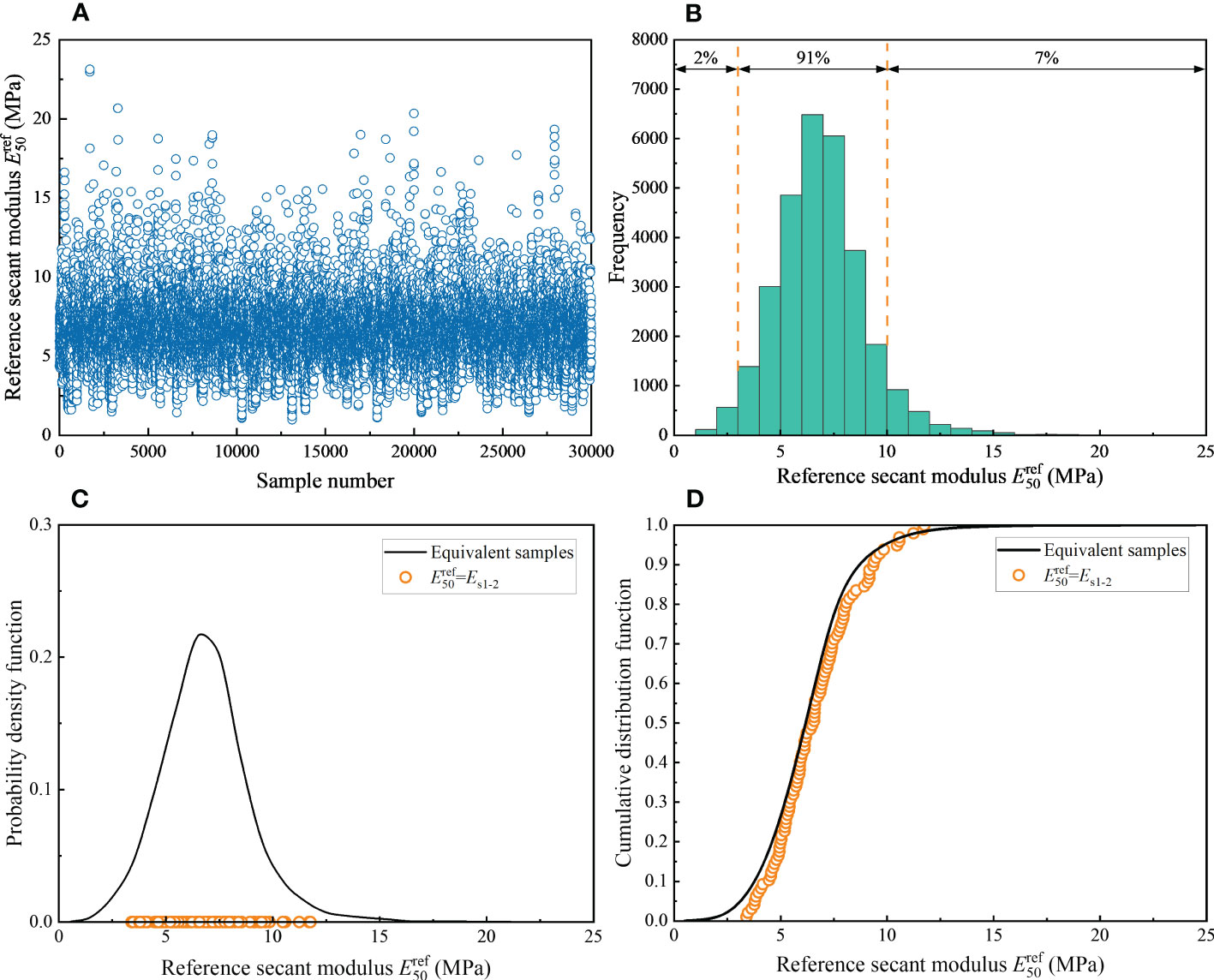
Figure 6 Probability distribution of $E_{50}^{\text{ref}}$: (A) Scatter plot. (B) Histogram. (C) Probability density function. (D) Cumulative distribution function.

The mean and standard deviation estimated from equivalent samples and empirically converted data are 6.9 MPa and 2.1 MPa, 6.7 MPa and 1.9 MPa, respectively. The mean difference between the equivalent samples and converted data is 0.2 MPa, and the standard deviation is 0.2 MPa, with deviations of 3.0% and 10.5%, respectively. The results indicate that $E_{50}^{\text{ref}}$ obtained by the two methods are in good agreement, especially the mean value. Suppose the mean value is chosen to be the characteristic value of $E_{50}^{\text{ref}}$. The final characteristic value of $E_{50}^{\text{ref}}$ from the Bayesian approach is 6.9 MPa.

4.2 Sensitivity analysis of Bayesian approach

4.2.1 Mean μ

The equivalent samples of $E_{50}^{\text{ref}}$ reflect the combined information of a prior knowledge and corresponding test data. Three groups of mean shown in Figure 7A are selected to study the influence of mean μ. All of them are uniform distribution, of which the second group has been used in Section 4.1 and will serve as the basis for the research. The Bayesian inversion results are shown in Figure 7B. As seen in the histogram, the final results obtained by μ∈[5.0, 7.0] and μ∈[3.9, 8.0] are closer, peaking at 6.5 MPa and 5.5 MPa in the center of the interval, respectively. The results obtained in the maximum interval range μ∈[1.6, 15.0] differ greatly from the two ranges mentioned above, reaching a peak at 13.5 MPa in the center of the interval. At the same time, the sample distribution ranges of μ∈[5.0, 7.0] and μ∈[3.9, 8.0] are consistent. Samples with a smaller prior range μ∈[5.0, 7.0] are more concentrated, and the sample size at the peak exceeds 7000. The large prior range of the mean value makes the final result deviate greatly from the true value of $E_{50}^{\text{ref}}$.

FIGURE 7

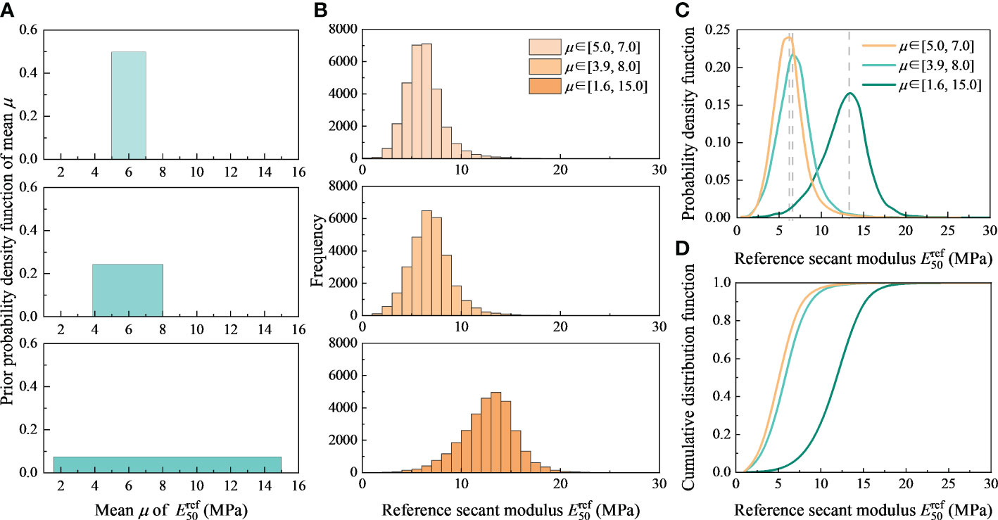
Figure 7 Sensitivity analysis of mean μ: (A) Three groups of μ. (B) Histogram. (C) Probability density function. (D) Cumulative distribution function.

The samples of sensitivity analysis were also used to estimate the probability density function and cumulative distribution function of $E_{50}^{\text{ref}}$, as shown in Figure 7C, D. The gray dashed line in the figure is the peak value, from which the results are consistent with the above analysis. Through the equivalent samples estimation, the final results of $E_{50}^{\text{ref}}$ obtained from μ∈[5.0, 7.0] and μ∈[3.9, 8.0] are 6.2 MPa and 6.9 MPa, with a deviation of 3.1% and 7.8% from 6.4 MPa in laboratory test, respectively. However, the results obtained from μ∈[1.6, 15.0], with a deviation almost doubled, significantly deviating from the acceptable error range of the parameter inversion results. The standard deviation of the three groups is 1.9MPa, 2.1MPa and 2.7MPa, respectively. The range of the mean value of $E_{50}^{\text{ref}}$ in this inversion is a relatively subjective judgment obtained by statistical analysis of a small amount of data. Its value range is derived from the statistics of $E_{50}^{\text{ref}}$ test values of soils in different regions. Therefore, better inversion results were obtained when the selected test values μ∈[3.9, 8.0] were chosen for the silty clay in each region. Narrowing this range gives more accurate results, such as μ∈[5.0, 7.0]. And when μ∈[1.6, 15.0], the increase in scope leads to ambiguity of information, resulting in unreasonable results. Therefore, a reasonable range of prior knowledge of soil parameters must be selected in practical application. Statistics of silty clay values in specific areas will greatly increase the reliability of the inversion results.

4.2.2 Standard deviation σ

Similar to the research of μ, the three groups of standard deviation are selected to explore the influence of σ, as shown in Figure 8A. Compared to the μ, the results of σ∈[0.5, 2.0], σ∈[0.5, 3.0] and σ∈[0.5, 8.0] have little difference in Figure 8B. The peaks are located close to each other, at 7.5 MPa, 6.5 MPa and 6.5 MPa in the center of the interval, respectively. Similarly, as the selected range of σ decreases, the obtained samples become more concentrated and the probability density function becomes steeper, reflecting that the accurate selection of the range of prior knowledge has a greater influence on the posterior distribution.

FIGURE 8

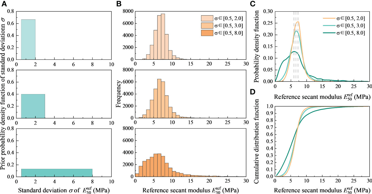
Figure 8 Sensitivity analysis of standard deviation σ: (A) Three groups of σ. (B) Histogram. (C) Probability density function. (D) Cumulative distribution function.

The equivalent samples are plotted as probability density function and cumulative distribution function, as shown in Figure 8C, D. It can be determined from the peak position that the change of σ range has less effect on the peak of $E_{50}^{\text{ref}}$ probability density function than μ. However, the change of σ range has a certain influence on the shape of probability density function, which gradually transitions from normal distribution to lognormal distribution. The estimated $E_{50}^{\text{ref}}$ for the three ranges is 6.9 MPa, 6.9 MPa, and 6.8 MPa, with deviations from laboratory test 6.4 MPa of 7.8%, 7.8%, and 6.3%, respectively. The standard deviation of samples estimation is 1.6MPa, 2.1MPa and 4.6MPa, respectively. From another perspective, the larger σ range makes the sample more discrete and changes more significantly than μ.

4.3 Deformation analysis of underwater shield tunnelling

4.3.1 Numerical model

PLAXIS was used to establish the numerical model of the Yellow River tunnel passing through the south embankment in this paper. To simplify the calculation, the following assumptions were made in the modelling process: (1) The silty clay stratum is homogeneous and isotropic; (2) Regardless of the longitudinal slope of the tunnel, the tunnel is laid horizontally; (3) The water level of the Yellow River is constant, and the seepage is neglected.

The model dimension is 360 m×150 m×100 m, the overburden depth of the tunnel is 40 m, and the shallowest section is 30 m below the Yellow River. A support pressure of 0.5 MPa is set in front of the tunnel face and increases with depth by 0.01 MPa/m. The tunnel advances in the Y-direction with every 10 m (5 rings) for a construction stage. The eastern line is constructed before the western line. The numerical model is shown in Figure 9.

FIGURE 9

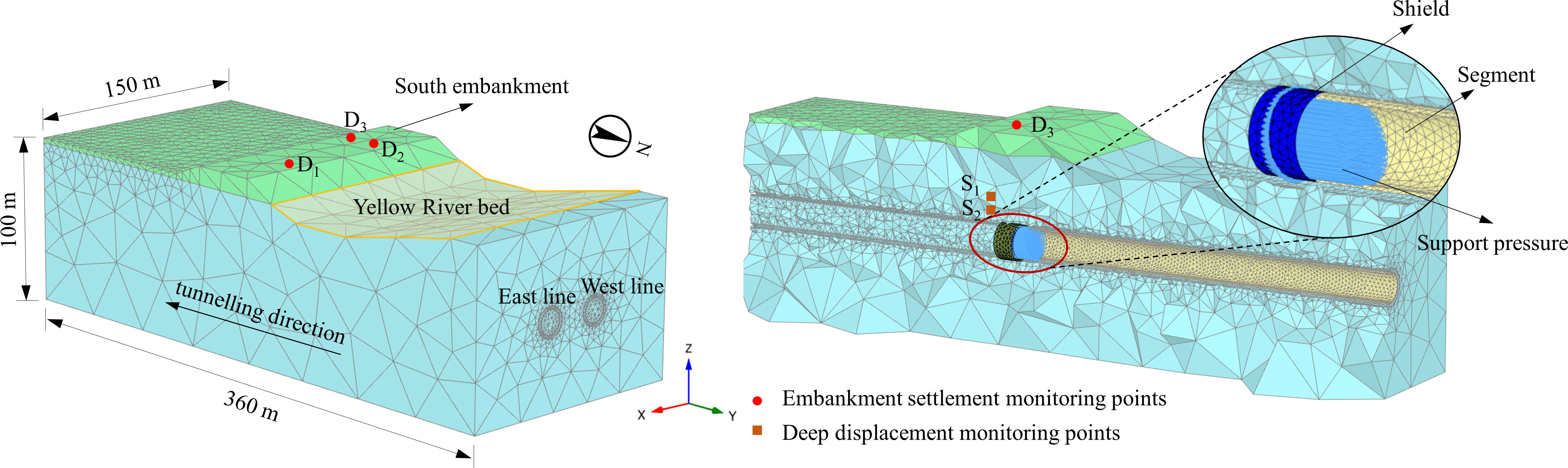
Figure 9 3D numerical model of the Yellow River tunnel passing through the south embankment.

The HSS model and elastic model were assumed for soil, shield shell and segment, respectively. Bayesian inversion result was used for the value of $E_{50}^{\text{ref}}$. The value of $E_{\text{oed}}^{\text{ref}}$ and $E_{\text{ur}}^{\text{ref}}$ was obtained from the empirical relationships, expressed as $E_{\text{oed}}^{\text{ref}}$= $E_{50}^{\text{ref}}$, $E_{\text{ur}}^{\text{ref}}$= 3 $E_{50}^{\text{ref}}$. And the other parameters were taken from the laboratory test, such as consolidation drainage test, standard consolidation test and resonant column test, or the default values. The Young’s Modulus E of segment is decreased to 80% of its initial value of 35.5 GPa, which is based on the tunnelling experience in China, to take into account the impact of joint on the stiffness of tunnel lining (Feng et al., 2011; Xie et al., 2016). The soil parameters are listed in Table 2.

TABLE 2

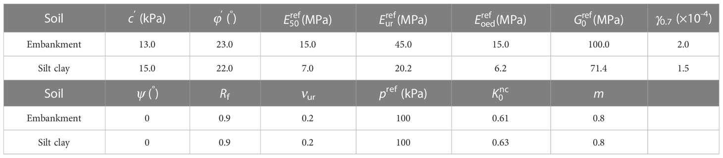
Table 2 Physical model parameters of soil.

4.3.2 Comparison between numerical simulation and field measurement

To further study the deformation caused by shield tunnelling, three monitoring points, D₁, D₂ and D₃, were set up at the top of the embankment section. Meanwhile, two deep settlement monitoring points, S₁ and S₂, were set at 30 m and 34 m below point D₃. The site monitoring point layout is also shown in Figure 9.

The monitoring and simulation results of the D₁, D₂ are shown in Figure 10A. It can be seen that the embankment settlement can be divided into three stages, which are the initial stage, rapid settlement stage and stable stage. According to the monitoring results, the support pressure applied in front of the tunnel face caused the monitoring sites D₁ and D₂ to heave. Compared with the field measurement, the simulation results of shield tunnelling did not show the phenomenon of surface heave. And the settlement started at the beginning of the tunnelling, but the settlement was almost negligible. When the shield tunnelling reached the vicinity of the monitoring point, both the simulated and monitored embankment settlement rates accelerated significantly and a large embankment settlement appeared. In this stage, the maximum settlement predicted by the monitoring and simulation is 5.5 mm and 6.5 mm, respectively, accounting for 65% and 90% of the total settlement. The difference between the two settlement is small, but the settlement proportion is large. This is because in the field measurement, there is the re-consolidation settlement after soil disturbance, and the settlement of this part is second only to the settlement generated by construction disturbance in the project. The rapid settlement stage (Stage 1) at point D₂ is longer, with a maximum settlement of 12 mm, accounting for more than 90% of the total embankment settlement. This indicates that the advanced construction of the east line greatly influences the stacking of the west line settlement, and the final settlement of the west line is greater than the east line. The settlement rate of monitoring points D₁ and D₂ in the rapid settlement stage is about 0.8 - 1.3 mm/d. Figure 10A also shows the results obtained from the non-inverted model, which can be seen to be larger than the measured and inverted results. It indicates that the non-inverted parameters underestimate the stiffness of the soil, resulting in a certain deviation in the calculation results. One issue should be addressed in Figure 10A. When the east line was excavated, the boundary settlement was about -6 mm. rather than 0 mm, as we find out in most field monitoring. The mesh size and the chosen soil model are both to cause this phenomenon. A smaller mesh size is typically required for the advanced soil model to obtain convergence results. However, a small mesh size will reduce computational efficiency and is unsuitable for large models. It is noted that the total settlement of monitoring point D₂ above the west line was higher than D₁ above the east line. This is because when the axis distance between the two tunnels is relatively close, the soil in the middle area of the two tunnels will be affected by two large-diameter shield construction disturbances. In this model, the results of measured maximum settlement at D₁ and D₂ are 8.5 mm and 13 mm, respectively. The numerical results are 7.3 mm and 10.5 mm, respectively.

FIGURE 10

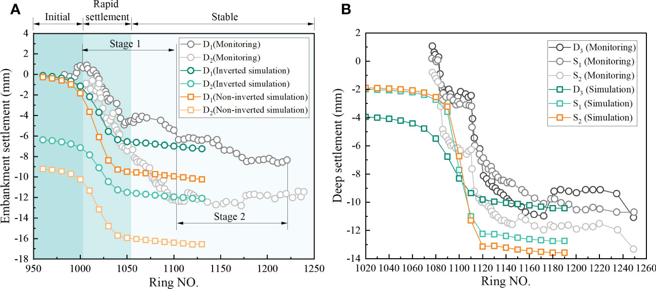
Figure 10 Comparison between field measurement and simulated result: (A) Embankment settlement of D₁ and D₂. (B) Deep settlement of D₃, S₁ and S₂.

The comparison of field measurement between monitoring points D₃, S₁ and S₂ in Figure 10B shows that the settlement trend of D₃ was roughly the same as that of S₁ and S₂. Among them, the settlement of the monitoring point S₂ closer to the tunnel (about 3 m) is more extensive, and the maximum settlement reaches -13.5 mm. The value and settlement rate of this monitoring point is greater than those of the other two. From the simulation results, the settlement changes of S₁ and S₂ are the same at the beginning of the tunnel excavation, and the amount of change is small. The settlement at D₃ is about 2 mm larger than the deep settlement. The settlement of the three monitoring points grows quickly when the tunnel is close to an embankment, and the deep settlement is more noticeable than the surface settlement. The maximum settlement of S₂ is slightly larger than S₁, and the ground settlement is the smallest. In terms of the total settlement of each stage, the measured monitoring point S₁, which is located around 7 m above the tunnel, is close to the monitoring point D₃ at the top of the embankment. The maximum settlement is -10.6 mm and -11.4 mm, respectively.

At the same time, the simulated settlement curve is about 10 rings ahead of the field measurement. This is because in numerical simulation, considering the horizontal and homogeneous soil layer, the set support pressure is a constant. In actual construction, due to the dynamic adjustment of construction parameters, the displacement near the tunnel surface caused by construction has been well controlled, and the affected range is smaller than the simulation results, resulting in lag in the measured results. The corresponding conclusion can also be drawn from the fact that the final simulation prediction result is larger than the actual measurement. In general, comparing numerical simulation and field measurement, it can be seen that the simulation results agree with the measurements, proving the viability of the method used to obtain the HSS model parameters from the CPTU data.

4.4 Influencing factors of river bed settlement

4.4.1 Support pressure

The soil disturbance caused by tunnel construction can be significantly reduced by using reasonable support pressure, avoiding engineering risks such as splitting and roof falling in shallow underwater soil sections and river water backflow. The actual support pressure set in the Yellow River tunnel project is mostly between 0.3 MPa - 0.6 MPa. Therefore, six analysis cases of 0.3 MPa, 0.35 MPa, 0.4 MPa, 0.45 MPa, 0.5 MPa and 0.55 MPa were selected.

Figure 11 shows the maximum riverbed settlement under different support pressures. When the support pressure is 0.3 MPa, the influence of soil displacement in front of the tunnel face has caused a large riverbed settlement, the maximum settlement is -8.9 mm. When pressure increases to 0.45MPa, the riverbed settlement is well controlled, and the maximum settlement is -2.0mm. Before 0.45MPa, the decrease rate was almost linear, and after 0.45MPa, the decrease rate slowed down. It can be seen that when the support pressure increases to a certain extent, the influence of support pressure on settlement control is limited. For this model, the optimal supporting pressure is between 0.45MPa and 0.5MPa.

FIGURE 11

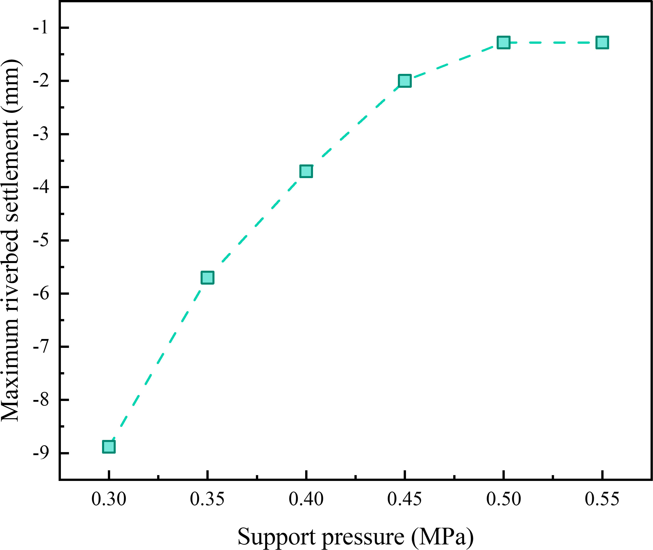
Figure 11 Maximum riverbed settlement at different support pressures.

4.4.2 Shield slope

The longitudinal slope of the shield tunnel is mainly controlled within 5^° in the design. However, the longitudinal slope may exceed the design value due to the complexity of geological conditions and the uncertainty of shield attitude control. Cheng et al. (2021) designed the longitudinal slope angle as 15^° to capture the tunnel failure mode more obviously in the small-size model test and verified it with numerical simulation. In most projects, the maximum longitudinal slope angle in practical application is usually less than 10^°. Therefore, +10^°, +5^°, 0^°, -5^°, -10^° were selected for comparative study.

Figure 12 shows the failure mechanism of the tunnel face at different slopes. When the slope angle of the tunnel is +10^°, the soil deformation extends to the ground, resulting in an extensive range of settlement trough. When the slope angle is +5^°, the range of settlement trough is smaller. The failure mechanism of a horizontal tunnel is similar to +5^°. In all cases of shield downslope, the deformation effects did not reach the surface. This condition is mainly determined by the horizontal projection area of tunnel on the ground. It is generally understood that the larger the projection area is, the larger the impact area of the tunnel excavation on the riverbed, which will lead to increased settlement.

FIGURE 12

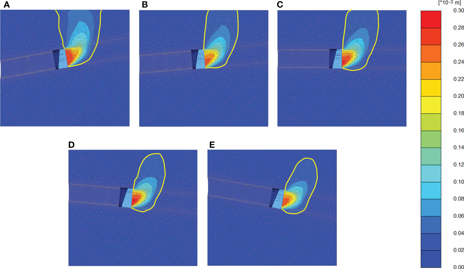
Figure 12 Failure mechanism at different slopes: (A) +10°. (B) +5°. (C) 0°. (D) -5°. (E) -10°.

Figure 13A shows the transverse riverbed settlement of different slopes at which the buried depth is 2D. The transverse riverbed settlement of the tunnel reaches its maximum value at the middle line of the tunnel. With the tunnel slope from +10^° to -10^°, the maximum transverse riverbed settlement is -25.8 mm, -20.8 mm, -17.0 mm, 13.4 mm and -11.1 mm, respectively. It is obvious that the uphill section will cause greater riverbed settlement than the downhill section.

FIGURE 13

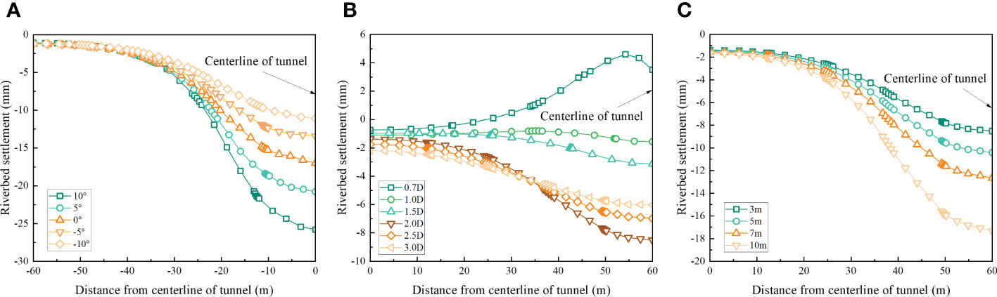
Figure 13 Transverse riverbed settlement under different influencing factors: (A) Shield slopes. (B) Buried depths. (C) Water levels.

4.4.3 Buried depth

Buried depth affects the tunnel construction deformation. Under the same condition, different buried depths will cause different stratum displacements. Generally, the shallowest buried depth of the tunnel should be greater than 0.7D (D refers to the outside diameter of the tunnel). And the buried depth of the Jinan Yellow River Tunnel is between 11.2 - 42.3m, about 0.7D - 2.8D. Based on this, six working conditions were selected: 0.7D, 1.0D, 1.5D, 2.0D, 2.5D and 3.0D.

Figure 13B shows the transverse riverbed settlement of different buried depths. Under the same conditions, when the buried depth is less than or equal to 2.0D, the riverbed settlement increases with the increase of the buried depth. Under 0.7D, the supporting pressure of 0.3 MPa has exceeded the sum of soil and water pressure. Most areas are uplifted, and the maximum uplifted is about 5.0mm. The transverse riverbed settlement of the tunnel at 1.0D is small, about -1.6mm at most. With the increase of tunnel buried depth, the maximum riverbed settlement reached -8.5mm at 2.0D. It is worth noting that the above phenomenon was studied only by changing the buried depth. In other words, the greater the buried depth, the smaller the support pressure ratio.

It can also be seen that when the tunnel buried depth is 2.5D and 3.0D, the maximum riverbed settlement no longer increases with the increase of buried deep, and the law is precisely the opposite. This is because when the buried depth is greater than 2.0D, the soil arch effect is generated in the upper soil, preventing the formation deformation caused by tunnel excavation transmitting to the riverbed, and the riverbed deformation is reduced.

4.4.4 Water level

Construction of underwater tunnels is challenging because they must withstand greater water pressure than conventional tunnels. The level of water not only affects the structural design of segments and waterproofing and plays a crucial role in the selection of construction parameters (Du et al., 2021). The water condition also restricts the implementation of various pretreatment measures. Before the Wuhan Yangtze River Tunnel, the maximum water pressure of the large-diameter shield built on the Huangpu River in Shanghai did not exceed 0.45 MPa. Subsequently, the maximum water pressure is constantly refreshed with the vigorous development of large-diameter shield tunnels.

Combined with the previous research, when the support pressure is 0.3 MPa, the water level of 3 m, 5 m, 7 m, 10 m, 20 m was selected for analysis. The calculation results are shown in Figure 13C. The riverbed settlement increases with the water level rise. This is because the change in water level in the model is equivalent to the uniform load of different sizes applied on the riverbed. In contrast, the high-water level represents that the model receives a greater vertical load, naturally increasing the riverbed settlement. The maximum transverse settlement caused by the 20 m water level is -54.1mm and -54.7mm, respectively. It indicates that the support pressure adopted cannot support the tunnelling, so the results are not shown.

5 Conclusions

In this work, the Bayesian probability characterization approach for the HSS model parameter $E_{50}^{\text{ref}}$ of silty clay was proposed. Also, deformation analysis induced by the underwater tunnel construction in the Jinan Yellow River Tunnel project has been performed. The analysis results from the numerical simulation are consistent with the monitoring data. In addition, this paper analyses the deformation response of underwater tunnel construction under different support pressures, shield slopes, buried depths and water levels. The following conclusions can be drawn:

(1) Based on the HSS model, the finite element analysis of cavity expansion during CPTU penetration was carried out, and the correlation model of the normalized cone tip resistance Q with the reference tangent modulus $E_{50}^{\text{ref}}$ and the effective internal friction angle φ^’ was established and verified using mini CPTU chamber test. It shows that the results obtained from the correlation model are all located near the test values and are relatively close to the test values of undisturbed soil, with a deviation of 4.9%, which verifies the applicability of the model in the CPTU penetration of silty clay.

(2) A Bayesian inversion approach for calculating the reference secant modulus $E_{50}^{\text{ref}}$ of silty clay in Jinan was presented based on the penetration data and the transformation model. The results show that the estimated $E_{50}^{\text{ref}}$ obtained by the Bayesian equivalent sample method is 6.9 MPa, which agrees with the laboratory test result of 6.4 MPa. With the decrease of the range selected by the prior information mean μ and standard deviation σ, the obtained samples will become more concentrated, and the probability density function will become steeper.

(3) The good agreement between the measurement and numerical simulation confirms that the parameters obtained by the Bayesian probability characterization approach considering the inherent variability of soil parameters and the uncertainty of the transformation model are reliable. This indicates that the proposed Bayesian probability characterization approach combined with CPTU can be applied to evaluate the law of riverbed settlement induced by underwater tunnelling construction.

(4) With the pressure increase, the maximum riverbed settlement gradually decreases, but there is an upper limit. The optimal support pressure of the established model is between 0.45 MPa and 0.5 MPa. With the tunnelling slope from +10° to -10°, the tunnel construction settlement trough gradually decreases. Under the same condition, before the buried depth is 2D, the riverbed deformation increases with the increase of the buried depth. After the buried depth exceeds 2D, the riverbed settlement decreases due to the soil arching effect. The riverbed settlement increases with the water level rise.

Data availability statement

The raw data supporting the conclusions of this article will be made available by the authors, without undue reservation.

Author contributions

YL: Conceptualization, methodology, software, investigation, data curation, writing – original draft, writing – review & editing. PY: Investigation, writing – review & editing. YZ: Conceptualization, writing – review & editing, funding acquisition. JC: Project administration. TL: Conceptualization, supervision, funding acquisition. HW: Data curation. HL: Supervision, project administration. All authors contributed to the article and approved the submitted version.

Funding

This work presented in this paper was supported by the National Natural Science Foundation of China (U2006213), the National Natural Science Foundation of China (42277139) and the Natural Science Foundation of China (42207172).

Acknowledgments

We appreciate the reviewers for their valuable comments, which are crucial to shaping our manuscript, at the same time, we are also grateful for the financial support provided by the above-mentioned funds.

Conflict of interest

Author JC is employed by China Railway 14th Bureau Group Corporation Limited.

The remaining authors declare that the research was conducted in the absence of any commercial or financial relationships that could be constructed as a potential conflict of interest.

Publisher’s note

All claims expressed in this article are solely those of the authors and do not necessarily represent those of their affiliated organizations, or those of the publisher, the editors and the reviewers. Any product that may be evaluated in this article, or claim that may be made by its manufacturer, is not guaranteed or endorsed by the publisher.

References

Burland J. B. (1989). Ninth laurits bjerrum memorial lecture: ''small is beautiful-the stiffness of soils at small strains. Can. Geotech. J. 26 (4), 499–516. doi: 10.1139/t89-064

CrossRef Full Text | Google Scholar

Cai G. J., Zou H. F., Liu S. Y., Puppala A. J. (2017). Random field characterization of CPTU soil behavior type index of jiangsu quaternary soil deposits. Bull. Eng. Geol. Environ. 76 (1), 353–369. doi: 10.1007/s10064-016-0854-x

CrossRef Full Text | Google Scholar

Cao Z. J., Wang Y., Li D. Q. (2016). Quantification of prior knowledge in geotechnical site characterization. Eng. Geol. 203, 107–116. doi: 10.1016/j.enggeo.2015.08.018

CrossRef Full Text | Google Scholar

Cao Z. J., Zheng S., Li D. Q., Phoon K. K. (2019). Bayesian Identification of soil stratigraphy based on soil behaviour type index. Can. Geotech. J. 56 (4), 570–586. doi: 10.1139/cgj-2017-0714

CrossRef Full Text | Google Scholar

Cheng C., Jia P. J., Zhao W., Ni P. P., Bai Q., Wang Z. J., et al. (2021). Experimental and analytical study of shield tunnel face in dense sand strata considering different longitudinal inclination. Tunn. Undergr. Space Technol. 113, 103950. doi: 10.1016/j.tust.2021.103950

CrossRef Full Text | Google Scholar

Ching J. Y., Phoon K. K. (2019). Constructing site-specific multivariate probability distribution model using Bayesian machine learning. J. Eng. Mech. 145 (1). doi: 10.1061/(ASCE)EM.1943-7889.0001537

CrossRef Full Text | Google Scholar

Du X., Sun Y. F., Song Y. P., Zhu C. Q. (2021). In-situ observation of wave-induced pore water pressure in seabed silt in the yellow river estuary of China. J. Mar. Environ. Eng. 10 (4), 305–317.

Google Scholar

Feng K., He C., Xia S. (2011). Prototype tests on effective bending rigidity ratios of segmental lining structure for shield tunnel with large cross-section. Chin. J. Geotech. Eng. 33 (11), 1750–1758.

Google Scholar

Huang X., Schweiger H. F., Huang H. W. (2013). Influence of deep excavations on nearby existing tunnels. Int. J. Geomech. 13 (2), 170–180. doi: 10.1061/(ASCE)GM.1943-5622.0000188

CrossRef Full Text | Google Scholar

Huang M., Zhan J. W. (2019). Face stability assessment for underwater tunneling across a fault zone. J. Perform. Constr. Facil. 33 (3), 04019034. doi: 10.1061/(ASCE)CF.1943-5509.0001296

CrossRef Full Text | Google Scholar

Jardine R. J., Potts D. M., Fourie A. B., Burland J. B. (1986). Studies of the influence of non-linear stress-strain characteristics in soil-structure interaction. Géotechnique 36 (3), 377–396. doi: 10.1680/geot.1986.36.3.377

CrossRef Full Text | Google Scholar

Likitlersuang S., Surarak C., Wanatowski D., Oh E., Balasubramaniam A. (2013). Finite element analysis of a deep excavation: a case study from the Bangkok MRT. Soils Found. 53 (5), 756–773. doi: 10.1016/j.sandf.2013.08.013

CrossRef Full Text | Google Scholar

Lin C. G., Zhang Z. M., Wu S. M., Yu F. (2013). Key techniques and important issues for slurry shield under-passing embankments: a case study of hangzhou qiantang river tunnel. Tunn. Undergr. Space Technol. 38, 306–325. doi: 10.1016/j.tust.2013.07.004

CrossRef Full Text | Google Scholar

Mo P. Q., Gao X. W., Yang W. B., Yu H. S. (2020). A cavity expansion-based solution for interpretation of CPTu data in soils under partially drained conditions. Int. J. Numer. Anal. Methods Geomech. 44 (7), 1053–1076. doi: 10.1002/nag.3050

CrossRef Full Text | Google Scholar

Ng C., Zheng G., Ni J. J., Zhou C. (2020). Use of unsaturated small-strain soil stiffness to the design of wall deflection and ground movement adjacent to deep excavation. Comput. Geotech. 119, 103375. doi: 10.1016/j.compgeo.2019.103375

CrossRef Full Text | Google Scholar

Phoon K. K., Kulhawy F. H. (1999). Characterization of geotechnical variability. Can. Geotech. J. 36 (4), 612–624. doi: 10.1139/t99-038

CrossRef Full Text | Google Scholar

Qiu D. H., Cui J. H., Xue Y. G., Liu Y., Fu K. (2019). Dynamic risk assessment of the subsea tunnel construction process: analytical model. J. Mar. Environ. Eng. 10 (3), 195–210.

Google Scholar

Randolph M. F., Dolwin J., Beck R. (1994). Design of driven piles in sand. Géotechnique 44 (3), 427–448. doi: 10.1680/geot.1994.44.3.427

CrossRef Full Text | Google Scholar

Sadrekarimi A. (2016). Evaluation of cpt-based characterization methods for loose to medium-dense sands. Soils Found. 56 (3), 460–472. doi: 10.1016/j.sandf.2016.04.012

CrossRef Full Text | Google Scholar

Suryasentana S. K., Lehane B. M. (2014). Numerical derivation of cpt-based p-y curves for piles in sand. Géotechnique 64 (3), 186–194. doi: 10.1680/geot.13.P.026

CrossRef Full Text | Google Scholar

Suzuki Y. (2015). Investigation and interpretation of cone penetration rate effects (The University of Western Australia).

Google Scholar

Tang S. H., Zhang X. P., Liu Q. S., Xie W. Q., Yang X. M., Chen P., et al. (2021). Analysis on the excavation management system of slurry shield tbm in permeable sandy ground. Tunn. Undergr. Space Technol. 113, 103935. doi: 10.1016/j.tust.2021.103935

CrossRef Full Text | Google Scholar

Tian M., Li D. Q., Cao Z. J., Phoon K. K., Wang Y. (2016). Bayesian Identification of random field model using indirect test data. Eng. Geol. 210, 197–211. doi: 10.1016/j.enggeo.2016.05.013

CrossRef Full Text | Google Scholar

Wang Y., Cao Z. J. (2013). Probabilistic characterization of young's modulus of soil using equivalent samples. Eng. Geol. 159, 106–118. doi: 10.1016/j.enggeo.2013.03.017

CrossRef Full Text | Google Scholar

Wang Y., Cao Z. J., Li D. Q. (2016). Bayesian Perspective on geotechnical variability and site characterization. Eng. Geol. 203, 117–125. doi: 10.1016/j.enggeo.2015.08.017

CrossRef Full Text | Google Scholar

Wang W., Wang H., Xu Z. (2012). Experimental study of parameters of hardening soil model for numerical analysis of excavations of foundation pits. Yantu Lixue/Rock Soil Mechanics. 33 (8), 2283–2290. doi: 10.16285/j.rsm.2012.08.006

CrossRef Full Text | Google Scholar

Wang L. Q., Xiao T., Liu S. L., Zhang W. G., Yang B. B., Chen L. C. (2023). Quantification of model uncertainty and variability for landslide displacement prediction based on Monte Carlo simulation. Gondwana Res. doi: 10.1016/j.gr.2023.03.006

CrossRef Full Text | Google Scholar

Xie X. Y., Yang Y. B., Ji M. (2016). Analysis of ground surface settlement induced by the construction of a large-diameter shield-driven tunnel in shanghai, China. Tunn. Undergr. Space Technol. 51, 120–132. doi: 10.1016/j.tust.2015.10.008

CrossRef Full Text | Google Scholar

Xu X. T. (2007). Investigation of the end bearing performance of displacement piles in sand (The University of Western Australia).

Google Scholar

Xu X. T., Lehane B. M. (2008). Pile and penetrometer end bearing resistance in two-layered soil profiles. Géotechnique 58 (3), 187–197. doi: 10.1680/geot.2008.58.3.187

CrossRef Full Text | Google Scholar

Zhang W. G., Hou Z. J., Goh A., Zhang R. H. (2019). Estimation of strut forces for braced excavation in granular soils from numerical analysis and case histories. Comput. Geotech. 106, 286–295. doi: 10.1016/j.compgeo.2018.11.006

CrossRef Full Text | Google Scholar

Zhao Z. N., Congress S., Cai G. J., Duan W. (2022). Bayesian Probabilistic characterization of consolidation behavior of clays using CPTU data. Acta Geotech. 17 (3), 931–948. doi: 10.1007/s11440-021-01277-8

CrossRef Full Text | Google Scholar

Zhou H. Z., Zheng G., He X. P., Wang E. Y., Guo Z. Y., Nie D. Q. (2020). Numerical modelling of retaining structure displacements in multi-bench retained excavations. Acta Geotech. 15 (9), 2691–2703. doi: 10.1007/s11440-020-00947-3

CrossRef Full Text | Google Scholar